Threshold of the CAPB That Can Be Attributed to Fiscal Consolidation Episodes in South Africa

Abstract

This paper investigates the threshold of the cyclical adjusted primary balance (CAPB) that can be attributed to fiscal consolidation in South Africa. The CAPB framework is used in the threshold autoregressive regime (TAR) from 1979 to 2022. The contribution of the paper is the estimation of the CAPB in the context of South Africa to find fiscal consolidation episodes. Moreover, we identify the threshold of CAPB that can be attributed to fiscal consolidation, which the available literature is silent on. The TAR, first-order derivative and dummy variables are employed to find thresholds that can be attributed to fiscal consolidation episodes. By doing so, we provide valuable insights into the underlying dynamics of fiscal consolidation in the country, which can help policymakers develop more effective strategies for managing fiscal consolidation episodes. We estimated the success of fiscal consolidation on government debt in South Africa. There is a threshold of −1.28168%, 1.9182%, and 1.9270% for the CAPB of total government revenue increase, government expenditure cut, and the CAPB as a sum of both revenue and expenditure, respectively. These thresholds are different from the threshold of 1.5% advocated in the literature. It is recommended that a country-based threshold be used to find fiscal consolidation episodes. No or less fiscal consolidation is needed, as it results in less chance of reduction in government debt. Fiscal authorities must establish and execute a strategy for managing domestic government debt to avoid increasing its risk.

1. Introduction

The thinking around fiscal consolidation is that government expenditure cuts and tax increases will result in a fall in debt. This is because, at present, forward-looking economic agents will anticipate a reduction in tax and interest rates. This will increase permanent income (refers to the average income that a person expects to earn over a long period, such as their lifetime). It considers not only the income that a person currently earns but also the income that they expect to earn in the future as well as crowding in investment. As such, there will be an increase in economic activities, leading to higher economic growth and higher tax collection that can be used to reduce government debt (Alesina and Ardagna 2010; Mankiw 2019). One of the broad measures of discretionary government intervention to reduce the government debt that defines fiscal consolidation episodes is the cyclically adjusted primary balance (CAPB). The measure is concerned with the identification of discretionary fiscal policy changes in tax and government expenditure by filtering out changes that are due to economic fluctuations in tax as well as government expenditure (Alesina et al. 2019). At a policy level in South Africa (SA), fiscal authorities have made policy interventions to curb government debt. These interventions include the Public Finance Management Act of 1999 (PFMA), which advocates expenditure control. Regarding government debt, SA adopted the Southern African Development Community (SADC) 2006 Protocol on Finance and Investment (PFI), which stipulates that all member countries should have a rate of government debt share to GDP that is equal to or below 60% (SADC 2006). In 2012, the government introduced the expenditure ceiling to constrain high government debt. As such, the government committed to limiting real expenditure growth to an average of 2.9% per year (National Treasury Republic of South Africa 2012). In 2013, the government introduced cost-containment measures and cut expenditures on noncore goods and services, which amounted to R1.5 billion between 2013 and 2014 (National Treasury Republic of South Africa 2013).

In 2014, the Financial and Fiscal Commission (FFC) recommended more fiscal consolidation stances to restore the fiscal position and reduce government debt (National Treasury Republic of South Africa 2014). The FFC recommendation outlined that “Fiscal consolidation can no longer be postponed. Ensuring continued progress toward a better life obliges the government to safeguard public finances by acting within fiscal limits that can be sustained over the long term. To do otherwise would risk exposing the country to a debt trap, with damaging consequences for development for many years to come” (MTBPS 2014). The Fiscal Responsibility Bill (FRB) was tabled for discussion in the parliament of SA in 2018. The bill seeks to introduce government expenditure cuts, limit new government borrowing, maintain an expenditure ceiling and eliminate wasteful expenditure (FRB 2018). In 2019, the International Monetary Fund (IMF), Standard and Poor’s, Moody’s, and Fitch stressed that SA needs to implement a credible fiscal strategy and fiscal consolidation to contain the rise in government debt. This recommendation came with concern that the country is faced with high government debt and that there is policy uncertainty (IMF 2020).

South African domestic government debt has reflected upward swings as well as downward swings from 1979 to 2022. The domestic government debt before democracy in 1994 is characterized by a variation cycle that ranges between 29% and 41.80% (SARB 2022). From 1979 to 1994, the mean value of domestic government debt was 32.03%. After 1994, domestic government debt increased until it reached a rate of 44.66% in 1999. Domestic government debt starts to follow a downward trend until it reaches the minimum value of 21.99%. However, domestic government debt increased drastically, surpassing the previous cycle rate of 41.8% in 1994 and at a rate of 42.22% in 2015 (SARB 2022). Domestic government debt continues to increase until it reaches a rate of 71.72% in 2021 (SARB 2022). This rate of 71.72% is the rate that is above the 60% threshold advocated by SADC countries, of which South Africa is a member (Buthelezi and Nyatanga 2018). The debate on cyclically adjusted primary balance (CAPB) has gained interest over the years in the effort to find a fiscal consolidation. However, no consensus on what threshold to be used can be attributed to fiscal consolidation episodes, including (Afonso 2010; Afonso et al. 2022b; Alesina and Perotti 1995, 1997; Alesina et al. 1998; Alesina and Ardagna 2010; Devries et al. 2011; Giavazzi and Pagano 1995; Guajardo et al. 2014; Romer and Romer 2010; Yang et al. 2015), among others. Broad measures of discretionary government intervention to reduce the government debt that defines fiscal consolidation episodes are the definition approach, CAPB, and the narrative approach. The definition approach defines fiscal consolidation or discretionary action by a change in the economic variable threshold, such as government debt and government deficit (Braz et al. 2019). A large change in these economic variables reflects that there was government intervention to change, which can be attributed to fiscal consolidation (Alesina and Ardagna 2010; Gupta et al. 2005; Schaltegger and Weder 2014). Alesina and Ardagna (2010) deemed discretionary fiscal consolidation episodes when the government debt share of GDP fell by 4.5%. Bergman and Hutchison (2010) argue that when government debt share to GDP falls by 5% from the initial value, this reflects discretionary fiscal consolidation episodes. Alesina and Ardagna (2013) note that discretionary fiscal consolidation episodes can be defined when the government debt share of GDP falls by 3.5% for at least two consecutive years. However, the cyclically adjusted balance (CAB) is the difference between the overall balance and the automatic stabilizers. Equivalently, it is an estimate of the fiscal balance that would apply under current policies if output were equal to potential (Guajardo et al. 2014). The CAPB Cyclically adjusted balance excluding net interest payments (Braz et al. 2019). The CAPB builds from the intuition of the definition approach of the threshold to find fiscal consolidation episodes or discretionary action. The case in point (Alesina and Ardagna 2010; Gupta et al. 2005; Schaltegger and Weder 2014) identifies fiscal consolidation episodes when CAPB improves by 1.5%. Zaghini (2001) identified fiscal consolidation episodes when CAPB improves by 1.6% for two successive years. The identification of fiscal consolidation can be found in economic variables such as those reflected in

Table 1. Definition approach to threshold.

Economic Variables	Description of the Definition of Fiscal Consolidation Using Economic Variables
Government debts share to gross domestic product	A 4.5% decrease in government debt share to the gross domestic product in $(t+1),(t+2),$ and $(t+3)$ (Alesina and Ardagna 2010). Mean less than 5% from the initial government debt share to GDP for 3 successive years (Alesina and Perotti 1995; Alesina and Ardagna 2010).
Government deficit	A fall of 2% below the initial rate for government deficit in $(t+1),(t+2),$ and $(t+3)$ (Alesina and Perotti 1995; Alesina and Ardagna 2010).
Economic Growth	Economic growth is higher for 2 successful years for the growth rate means of cases where there was a fiscal consolidation (Alesina et al. 1998). The average economic growth rate at, $\left(t\right)$ is higher than, $(t-1)$ and $(t-2)$ (Giudice and Turrini 2007).
The cyclically adjusted primary balance	If there is a 1% change in the cyclically adjusted primary balance in 3 years (Tavares 2004). The cyclically adjusted primary balance improve by 1.5% in $\left(t\right)$ (Alesina and Perotti 1997; Alesina et al. 1998; Alesina and Ardagna 2010; Gupta et al. 2005; Hernández De Cos and Moral-Benito 2013; Schaltegger and Weder 2014). The cyclically adjusted primary balance improve by 1.5% in $(t+1)$ and $(t+2)$ (Alesina et al. 1998). The cyclically adjusted primary balance increased by 2% in $(t+1)$ (Alesina et al. 1998). The cyclically adjusted primary balance improves by mean $(\mu )$ plus standard deviation $\left(\sigma \right)$ in $\left(t\right)$ (Yang et al. 2015). The cyclically adjusted primary balance increase by the mean, $(\mu )$, plus standard deviation, $\left(\sigma \right)$, in $\left(t\right)$ (Yang et al. 2015).

The authors’ processing of the table above.

, namely, government debt share to gross domestic product, government deficit, economic growth, and cyclically adjusted primary balance. The narrative approach outlines that to identify fiscal consolidation episodes, one needs to go to the government document and obtain where it is stipulated that there will be a government expenditure cut and tax increase (Devries et al. 2011).

The problem that this paper identifies is that there is no specific rate or threshold as to how much improvement in CAPB, fall in government debt, and deficit can be attributed to fiscal consolidation episodes. The thresholds in the literature are defined by a large change in CAPB and government debt. The thinking is that large rates best represent exogenous or discretionary changes in fiscal policy since they are not close to economic fluctuation (Alesina and Perotti 1997; Yang et al. 2015)1. However, scholars have used different rates without effectively explaining how large is large and how to obtain this large value reflecting fiscal consolidation episodes. Given the fact that there is no agreement on the specific rate to be used, this may result in different fiscal consolidation episodes being identified even if scholars use the same data. As such, scholars will have different results and conclusions. Thus, there is no consensus on the threshold and an effective method to obtain larger values. Moreover, thresholds are not defined to decrease domestic government debt as advocated by the narrative approach (Devries et al. 2011). The scope of this paper is on a country based in South Africa. South Africa is selected to find evidence in the emerging economy other than looking at the advanced economy, which has been looked at by other scholars. Moreover, South Africa is preferred given that the country has shown interest in the adoption of fiscal consolidation. The objective of this paper is to investigate the threshold of the cyclical adjusted primary balance that can be attributed to fiscal consolidation episodes in South Africa. Given the background of fiscal consolidation, rationale, definition, and the problem identified above, the key economic question of this paper is, what is the threshold of the CAPB that can be attributed to fiscal consolidation? What is the impact of fiscal consolidation through government expenditure cuts and tax increases on government debt? Does fiscal consolidation reflect success in reducing government debt? Given the questions of this paper, the hypotheses are as follows:

Null:

There is a threshold of the cyclical adjusted primary balance that can be attributed to the fiscal consolidation episode.

Alt:

There is no threshold of the cyclical adjusted primary balance that can be attributed to the fiscal consolidation episode.

Null:

There is fiscal consolidation though government expenditure cuts and tax increases that impact government debt.

Alt:

There is no fiscal consolidation though government expenditure cuts and tax increases that impact government debt.

Null:

There is fiscal consolidation that reflects success in reducing government debt.

Alt:

There is no fiscal consolidation that reflects success in reducing government debt.

The rest of the paper has the following. First, Section 2 outlines the literature review and examines the fiscal consolidation measures and threshold fiscal consolidation empirical work that has been undertaken by scholars. Second, Section 3 discusses the methodology. Third, Section 4 discusses the empirical results. Finally, Section 5 outlines the conclusion of the paper.

2. Literature Review

2.1. Measures of Fiscal Consolidation

The rationale of fiscal consolidation is that government expenditure cuts and tax increases will result in a fall in government debt. This is because forward-looking economic agents will anticipate a reduction in tax and interest rates. This will increase permeant income, crowed in investment, increase economic activities, and higher tax collection that can be used to reduce government debt (Alesina and Ardagna 2010; Mankiw 2019). The Organization for Economic Co-operation and Development (OECD) and International Monetary Fund (IMF) reaction unction of fiscal authorizes that can be attributed to discretion action of fiscal consolidation in CAPB. The OECD and IMF used the elasticity of government expenditure and tax to find the discretionary action of fiscal consolidation.

$$\mathsf{\Delta }CAP{B}_t=\sum _{j=1}^4{TG{R}_{j,t}\left(\frac{y_t}{Y_t}\right)}^{{\epsilon }_{tgr}}-G_t{\left(\frac{y_t}{Y_t}\right)}^{{\epsilon }_g}$$

(1)

where $y$ is the nominal GDP and $Y$ is the nominal GDP potential2, which is estimated based on country-specific production functions. The OECD and IMF approach offers a much broader scope of CAPB since it involves a disaggregated approach and the elasticity of ${\epsilon }_{tgr}$ tax revenue and ${\epsilon }_g$ government expenditure (Mourre et al. 2013). There are four tax revenue categories shown in Equations (2)–(5).

$$\mathsf{\Delta }CI{T}_t={\mathsf{\beta }}_0+{\mathsf{\beta }}_{1}CI{T}_t\left(\frac{y_t}{Y_t}\right)+{\mathsf{\mu }}_t$$

(2)

$$\mathsf{\Delta }PI{T}_t={\mathsf{\beta }}_0+{\mathsf{\beta }}_{1}PI{T}_t\left(\frac{y_t}{Y_t}\right)+{\mathsf{\mu }}_t$$

(3)

$$\mathsf{\Delta }SS{C}_t={\mathsf{\beta }}_0+{\mathsf{\beta }}_{1}SS{C}_t\left(\frac{y_t}{Y_t}\right)+{\mathsf{\mu }}_t$$

(4)

$$\mathsf{\Delta }I{T}_t={\mathsf{\beta }}_0+{\mathsf{\beta }}_{1}I{T}_t\left(\frac{y_t}{Y_t}\right)+{\mathsf{\mu }}_t$$

(5)

The economic variables that are considered by the OECD and IMF approaches are presented in Equations (2)–(5), where $CIT$ is corporate income tax or companies’ tax $PIT$ is personal income tax, $SSC$ is social security contributions and $IT$ is indirect taxes. On the expenditure side is $umplb$ unemployment benefits shown in Equation (6).

$$\mathsf{\Delta }\frac{{UNE}_t}{{UNE}_{t-1}}={\beta }_0+{\beta }_1{unmplb}_t\left(\frac{y_t}{Y_t}\right)+{\mu }_t$$

(6)

where ${UNE}_t$ reflects unemployment and ${UNE}_{t-1}$ is unemployment in the last period and represents the $\mathsf{\Delta }$ change.

2.2. Threshold of Fiscal Consolidation

Alesina and Perotti (1995) defined the success of fiscal consolidation as changes in fiscal policy that are very tight, resulting in a gross debt share to GDP threshold that is 5% lower than the initial time. There were 66 successful fiscal episodes from 20 OECD countries between 1990 to 1992, and 14 episodes were very tight. Blanchard (1990) filtered out the cyclical movement to find a dictionary change that can be attributed to fiscal consolidation. Using a vector autoregressive (VAR) model, 14 OECD countries from 1970 to 1985 it was found that in very tight years, taxes increased by 1.2% of GDP, and spending was cut by 0.79% of GDP. The success of fiscal consolidation is possible when implemented mainly through government expenditure cuts. Giavazzi and Pagano (1995) used a definition approach in 20 Europe countries from 1970 to 1990, fiscal consolidation is deemed when there is a cumulative change in the CAPB that is at least 5%, 4%, and 3% points of GDP in years 4, 3, and 2. They found 223 fiscal consolidation episodes using this definition. It was noted that countries in the 1990s were adopting government expenditure cuts and tax increases to reduce the government debt ratio to gross domestic product. The definition of a fiscal consolidation episode by McDermott and Wescott (1996) was based on the threshold of a 1.5% increase in GDP over 2 years in 21 OECD countries from 1970 to 1995. There were 74 episodes based on revenue increases and 34 based on expenditure cuts. In a probit model, it was found that government expenditure cuts of government wages result in a 3.22% fall in government debt. These results suggest that government expenditure cut-based fiscal consolidations are more likely to be successful in reducing government debt. The CAPB threshold of a 2% or 1.05% increase in the share of GDP for two consecutive years by Alesina et al. (1998) in 18 OECD countries from 1965 to 1995 was undertaken as the rationale in the effort to define fiscal consolidation episodes. The fiscal consolidation was deemed to be successful if the primary deficit had a threshold that was 2% below the GDP in the year of the tight policy. Using these thresholds, the authors found 51 fiscal consolidation episodes, 19 of which were deemed to be successful, while 23 had an expansionary effect on economic activities in OECD economies characterized by low unemployment. Duperrut (1998), in South Africa from 1973 to 1997, fiscal adjustments were defined as a one-year improvement in the primary balance of the general government of more than 1.5% of GDP. It was found that there are episodes with two successfully representing 22.22% success. If the fiscal adjustment is of reasonable size, there is between a 1.5% and 2% negative impact on GDP. Hansen (2000), authors defined the success of the fiscal adjustment when the CAPB threshold improves by 2.5% or there is an improvement by 2% for at least two consecutive years in 18 OECD from 1980 to 1998. It was found that there are 39 fiscal consolidation episodes. The authors used the OLS model and found a 4.55% fall in government debt share to GDP in the representation of fiscal consolidation programs in OECD countries. Contrary to (Alesina and Ardagna 2010; McDermott and Wescott 1996), fiscal adjustments through the increase in taxes were found to contribute to the reduction of government debt.

Zaghini (2001) identified the fiscal consolidation episode and the CAPB increase with thresholds of 1.6% or 1.4% in 14 European countries from 1970 to 1998. The author found 100 fiscal consolidation episodes, of which 52 were characterized by a more expansionary fiscal contraction effect, while 48 were loose policy interventions. Using the VAR model, government debt increased by 3.7% with no fiscal consolidation intervention. Purfield (2003), fiscal adjustments and successful fiscal episodes were selected if there was a threshold of a 2% fall in government debt share to GDP in one year in 24 countries from the Soviet Union (FSU) and Eastern Europe (CEE) from 1992 to 2000. There were 33 fiscal adjustments with 27 fiscal consolidations based on government expenditure cuts. The VAR showed that a 1% fall in government expenditure cut resulted in a 2.3% increase in real GDP growth. However, a 1% increase in government tax results was found to result in a 2.1% increase in real GDP growth. Gupta et al. (2005), fiscal consolidation episodes were selected if the CAPB improved by the threshold of 1.25% of GDP for two cumulative years in 15 emerging economies from 1990 to 2000. It was found that fiscal consolidation lacked a positive impact on economic growth. However, the authors pointed out that the CAPB cannot identify the discretionary fiscal policy. Afonso et al. (2006), fiscal consolidation was identified if government debt falls by the threshold of 2%, and then the dummy variable was used. The authors found 114 and 20 successful fiscal consolidation episodes from 1990 to 2004. The logit model provided evidence that government expenditure-based fiscal consolidation results in a 4.2% fall in government debt.

Ardagna et al. (2007), authors defined fiscal adjustment as when CAPB improves a threshold of 1.5% and after 2 years government debt shares to GDP fall in 17 OECD countries from 1960 to 2002. The Logit model was adopted, and it was found that with a 1% increase in government expenditure cut and a tax increase, there is a 0.27% and a 0.30% chance of the fall in government debt share to GDP, respectively. Similar to (Afonso et al. 2006; Gupta et al. 2005; McDermott and Wescott 1996; Zaghini 2001), it was found that fiscal adjustment through government expenditure cuts leads to higher GDP growth rates than tax increases. Morris and Schuknecht (2007) adopted the VAR model, and fiscal consolidation episodes were selected when the CAPB increased by the threshold of 1.25% of GDP for two years in 16 OECD countries from 1960 to 2005. It was found that a 1% increase in CAPB results in a 0.6% increase in structural budget balance as a share of GDP. The author outlined that the CAPB has significant shortfalls of influence coming from cyclical changes. Contrary to (Alesina and Perotti 1995; Blanchard 1990) and (Gupta et al. 2005), the authors proposed that both short and longer asset prices need to be accounted for in the cyclically adjusted balance. Alesina and Ardagna (2010) used the definition of fiscal consolidation when there is a CAPB threshold of 1.5% of GDP in OECD countries similar to that of (McDermott and Wescott 1996). They found 107 periods of fiscal adjustments, which represented 15.1% of the observations, and 91 periods of fiscal stimuli, which were 12.9% of the observations in a sample from 1960 to 1994. It was also found that fiscal adjustments based upon spending cuts and tax increases are more likely to reduce deficits and debt over GDP ratios than those based upon tax increases. Barrios et al. (2010) used the fiscal consolidation episode definition adopted from the Alesina and Perotti (1995) and Alesina and Perotti (1997) criteria. The data reflected 235 fiscal consolidation episodes, the probit model was used, and it was found that there is a 30.3% and 24.4% chance that government debt will be lower than usual during the financial crisis and post-financial crisis in the presence of fiscal consolidation, respectively. Such results indicated that countries must have an effective model to implement fiscal consolidation in times of fiscal distress to increase the chances of success.

Romer and Romer (2010) and Devries et al. (2011) investigated fiscal consolidation from 1947 to 2006. They note that when fiscal consolidation is defined with the use of CAPB. This may lead to biased results since the CAPB is subjected to changes in the cyclical component. When the cyclical component is not accounted for, the CAPB may not be effective in finding fiscal consolidation or discretional action by fiscal authorities toward reducing government debt. As such, Romer and Romer (2010) and Devries et al. (2011) proposed that there is a need to go to a government document and extract where it is said there will be a cut in government expenditure and tax increase and take that a fiscal consolidation. Tagkalakis (2011), asset price impacts the CAPB. Using the VAR model, it was found that a 1% increase in asset prices results in 0.056% in government expenditure in 17 OECD countries from 1970 to 2005. This reflects that the CAPB may have the weakness of being affected by cyclical components such as asset prices. Similar to Tagkalakis (2011), Perotti (2012) investigated austerity and noted that CAPB has two possible limitations, namely, cyclical adjustments and asset price influence, which the author refers to as imperfect cyclical adjustment problems. Moreover, there are limitations when the CAPB is correlated with cyclical changes. The author concluded that the narrative approach of Romer and Romer (2010) and Devries et al. (2011) is better to avoid the above limitation note above, but the cyclically adjusted balance is flawed by both.

Aizenman et al. (2012) found in the VAR model that an increase in a value-added tax increase as an influence of fiscal consolidation reduces output. Perotti (2012) used the narrative approach advocated by Romer and Romer (2010) to find fiscal consolidation. Similar to Aizenman et al. (2012), it was found that VAT results in a fall in economic growth. Amo-Yartey et al. (2012) adopted a logit model as used by Afonso et al. (2006) and used economic data from CAPB. Fiscal consolidation was defined as a 1% improvement in CAPB in year one. They found 206, 107 similar to Alesina and Ardagna (2010), and 51 episodes of government debt share to GDP reduction. Fiscal consolidation increased the likelihood of government debt share to GDP reduction by 0.58%. Amo-Yartey et al. (2012) study demonstrates that significant debt reductions are linked to robust economic growth and effective and long-lasting fiscal consolidation initiatives from 1980 to 2011 in the Caribbean. Since growth is essentially nonexistent in the current context, severe budgetary austerity is unavoidable in the area. The obvious areas to cut back on spending include the public wage bill, public sector efficiency, and transfer payments. On the revenue side, there is plenty of potential for tax spending cuts, distortion elimination, and tax base expansion. To increase competitiveness, a comprehensive debt reduction strategy that includes changes to tax laws and structural reforms is required to go along with fiscal austerity. Heylen et al. (2013) built upon the scope of Heylen and Everaert (2000) and argued that changes in the government debt share to GDP between the range of 10% and 25% cannot be limited to either ‘success’ cases or ‘failures’, as there is a need to explain such outcomes. They found the change in the government debt share to GDP to vary between −25% and 35%. The OLS model was used, and it was found that a 1% increase in government efficiency increases the expansionary fiscal adjustment variable by 2.55%. Alesina and Ardagna (2013) identified the threshold of fiscal consolidation episodes to be successful if the debt-to-GDP ratio falls for two years after fiscal adjustment. This definition found 25 fiscal consolidation episodes of successful fiscal adjustments and 24 unsuccessful ones in 21 OECD countries from 1970 to 2010. This definition selects 35 episodes of expansionary fiscal adjustments and 17 contractionary adjustments. Heylen et al. (2013), used the definition of Alesina and Ardagna (2010) and the narrative definition of Devries et al. (2011) in 21 OECD countries. Using the panel instrument variable (IV) model, fiscal consolidation was found to be successful in reducing government debt. Yang et al. (2015) investigated the macroeconomic effects of fiscal adjustment using two approaches: the narrative and CAPB from 20 OECD countries from 1970 to 2009. In response to the estimation challenges of CAPB, they considered the asset price as mentioned by Romer and Romer (2010) and Devries et al. (2011). The authors account for asset price movement and remove its cyclical effect on government revenue. Moreover, contrary to the literature, they used the standard deviation in the fiscal consolidation definition to account for country-specific heterogeneity. They defined fiscal adjustment episodes as CAPB increases of 0.33 points of the mean and standard deviation for two and three years or more. There were 66 fiscal episodes, 11 of which lasted for one year, and the overall period of the 66 fiscal episodes was 19 years, with most of the countries having implemented fiscal consolidation for 9 years. The adopted panel Logit model found that expansionary fiscal adjustments result in a 28.9% likelihood of a decrease in economic growth. However, the lagged effect of such changes provides a 15% chance of an increase in the impact on economic growth. They then concluded that there is no clear evidence of the effect of fiscal consolidation.

Wiese et al. (2018) result shows that the effectiveness of fiscal changes is unrelated to their composition in 20 OECD countries from 1965 to 2015. With one exception, we show that political-economic variables are not strongly associated with effective fiscal adjustments. If left-wing governments concentrate on spending reductions and right-wing governments rely on tax hikes, the likelihood of a successful fiscal adjustment will rise. Arestis et al. (2018) note that debt sustainability hinges on the stability of the debt-to-GDP ratio other than fiscal consolidation. David and Leigh (2018) investigated a new action-based dataset of fiscal consolidation in Latin America and the Caribbean (LAC) using Romer and Romer (2010) definition of fiscal actions using a narrative approach. The rationale was to find discretionary changes in taxes and government spending primarily motivated by a desire to reduce the budget deficit and long-term fiscal health and not by a response to prospective economic conditions. The author examined contemporary policy documents, including budgets, central bank reports, and IMF and OECD reports. Based on this approach, it was found that there are 76 fiscal policy adjustments in 14 LAC economies. It was found that fiscal consolidation consisted of 0.9. Afonso and Silva Leal (2019) assess how fiscal elasticities vary during fiscal episodes in 20 OECD countries from 1970 to 2015. According to the results, positive “tax revenue” elasticities indicate that consumers have Ricardian behaviour. There were 182 found using the narrative approach and the threshold of 1.5% CAPB. There was an 18.61% chance of success of fiscal consolidation. Agnello et al. (2019) findings demonstrate that disparities in the duration and success/failure of fiscal consolidations are explained by economic and political factors, the amount and typology of fiscal adjustments, and the incidence of crises in 10 OECD countries from 1980 to 2010. Moreover, fiscal adjustment programs that succeed show a positive length dependence. Aye (2019) employed the narrative technique to measure fiscal consolidations in 14 Organization for Economic Co-operation and Development (OECD) nations between 1978 and 2014, using the criterion of a 2% change in the CAPB. It was discovered that tax hikes had little effect on public approval of the government, but spending cuts have the opposite effect, especially during economic downturns. Nunes (2019) in OECD nations between 1978 and 2017 noted that public spending before a fiscal consolidation has a positive effect on the likelihood that the fiscal consolidation will be successful; that is, the more public spending occurs in the year before a fiscal consolidation, the more likely it is that the fiscal consolidation will be successful, assuming all other factors remain constant. This finding may be consistent with the literature’s finding that expenditure-based fiscal consolidations are more likely to be successful.

Glavaški and Beker-Pucar (2020) investigated episodes of fiscal using the autoregressive distributed lag (ARDL) model from 1950 to 2018. It was found that the cyclically adjusted primary budget balance in GDP increases by 1%, and the real economic growth in western China will grow by 0.26%. This means that fiscal consolidation has a positive impact on economic growth in this region. de Rugy and Salmon (2020) investigated large fiscal consolidations in 26 countries from 1995 to 2018 and found 35 fiscal consolidation episodes. There were 62 successful consolidations found and 73 unsuccessful consolidations. They found that there were 45 expenditure-based fiscal consolidations (EB) episodes, and more than half were successful, while there were 67 tax-based fiscal consolidations (TB) episodes in which less than 4 in 10 were successful. Deskar-Škrbić and Milutinović (2021) results indicate that the fiscal consolidation implemented during the excessive deficit procedure is not growth-friendly and that it was partially self-defeating. This result was found in Croatia using the data from 1975 to 2018. Xiang et al. (2021) use the definition of Alesina and Perotti (1995) and Alesina and Perotti (1997) for fiscal consolidation in 13 Latin America. They found 51 fiscal consolidation episodes in 13 LAC countries. Using the panel multiple regression model, it was found that on average, these fiscal consolidation episodes have a statistically significant negative impact on total factor productivity (TFP). Moreover, they noted that in fiscal consolidation policies, expenditure cuts are a better policy option than tax increases, which agrees with the popular opinion in this field of research. Afonso et al. (2022a) investigated the non-Keynesian effects of fiscal austerity using different definition approaches from Alesina et al. (1998), Giavazzi and Pagano (1995), and Afonso and Jalles (2013). It was found that there are 122 episodes. Fiscal consolidation of tax increases has a positive effect on private consumption in the presence of fiscal consolidation. Bamba et al. (2020) found that fiscal consolidations significantly reduce the government investment-to-consumption ratio in 56 developed and emerging countries from 1975 to 2018. They define fiscal consolidation if the ratio CAPB/GDP improves each year, and the cumulative improvement is at least 2% to 3%. It was found that 52.85% were tax-based and 30.89% were expenditure-based. In 18 countries of the Euro area over the year 1999 to 2017, Carnazza et al. (2020) proposed a way to dispense with the estimation of potential GDP and, therefore, of the NAWRU to compute the CAPB and simultaneously focus only on the budgetary items, both revenues and expenditures, that automatically react to the business cycle. The idea is to choose the budgetary items whose cyclical component is significantly correlated with the cyclical component of GDP.

Giesenow et al. (2020) found that the frequency and duration of fiscal adjustments and expansions are influenced by political and institutional factors using the annual data for 60 countries from 1980 to 2014. The findings further emphasize how crucial it is to consider both the likelihood and durability of fiscal events. Ardanaz et al. (2020) found 42% and 41% of the tax base as well as expenditure-based fiscal consolidation in Latin America from 1985 to 2018. Moreover, fiscal consolidations do not have significant electoral consequences. Kalbhenn and Stracca (2020) noted that an increase in the CAB takes place with a public debt-to-GDP ratio already above 90% of GDP. This was using the 26 European Union countries on annual data between 1997 and 2017. Moreover, the authors found that economic agent opinion and credibility matter for the success of fiscal consolidation. In 14 European Union countries over the period 1970 to 2019, Quaresma (2021) combine the narrative technique with the standard CAPB method for identifying fiscal consolidations and extends this method to incorporate dummy variables for identifying monetary expansions. Few non-Keynesian effects are evident when fiscal consolidation is coupled with monetary expansion; therefore, monetary expansions do not necessarily explain the occurrence of expansionary fiscal consolidations. Afonso et al. (2022b) used the WEO-based CAPB, which is the world economic outlook data based on the International Monetary Fund (IMF) with a sample of 174 countries between 1970 to 2018. They applied the approach of a 1.5% increase in the CAPB to the identification of fiscal consolidation episodes. It was a fiscal consolidation program that implies an improvement in the degree of public financial sustainability in advanced and developing economies. Kopecky (2022) note that spending reductions and tax increases have different effects on demographics, with significant differences occurring between dependent and working-age groups in 17 OECD countries. When using Devries et al. (2011) data set Kopecky (2022) found that tax hikes result in a reduced output response in economies that are still developing, a stronger reaction as population weights shift toward middle age, and a falling response when there are high proportions of retirees. Using panel data of 73 countries over the 2003 to 2013 period Gootjes and de Haan (2022) note that fiscal laws increase the likelihood that fiscal changes will be successful, but only when there is enough transparency. These results seem to be highly resistant to the inclusion of contextualizing variables that might affect the effect of fiscal regulations and budget transparency. However, it is crucial to take into consideration the volatility of fiscal policy to identify the impact of fiscal laws on fiscal adjustments.

In panel of 21 emerging market and developing economies (EMDEs) from 2000 to 2018 by David et al. (2022) note that in the counterfactual scenario when spreads do not react to announcements, production is reduced by 30%. These findings demonstrate that a crucial conduit for the transmission of changes in fiscal policy is confidence impacts, which manifest as lower sovereign spreads. Furthermore, the importance of confidence effects grows with spread levels. Therefore, countries with high spread levels stand to gain the most from implementing credible austerity measures.

Table 2. Summary of fiscal consolidation episodes.

Author	Definition	EB	TB	TE	TS	% S
Alesina and Perotti (1995)	Threshold of 1.5% CAPB	59	60	119	66	55.46%
Alesina and Perotti (1997)	Changes in the CAPB that are at least 5%	125	98	223	43	19.28%
McDermott and Wescott (1996)	Threshold of 1.5% CAPB	34	74	108	43	39.81%
Alesina et al. (1998)	Threshold of 2% CAPB	23	28	51	19	37.25%
Zaghini (2001)	Threshold of 1.6% or 1.4% of CAPB	52	48	100	52	52.00%
Afonso et al. (2006)	Threshold of 2% CAPB			72	20	27.78%
Alesina and Ardagna (2010)	Threshold of 1.5% CAPB			107	91	85.05%
Barrios et al. (2010)	Threshold of 1.5% CAPB			235	71	30.21%
Amo-Yartey et al. (2012)	1% improvement in CAPB			107	51	47.66%
Alesina and Ardagna (2013)	Debt to GDP ratio falls 2 years	17	35	107	25	23.36%
Yang et al. (2015)	Narrative approach			66	19	28.79%
de Rugy and Salmon (2020)	Debt-to GDP ratio declines by at least 5 percentage points	45	67	112	66	58.93%
Ardanaz et al. (2020)	Narrative approach and threshold of 1.5% CAPB	41%	42%			56.6%
Nunes (2019)	Threshold of 1.5% CAPB	113	63			55%
Afonso and Silva Leal (2019)	Threshold of 1.5% CAPB			51		18.61%
Quaresma (2021)	Threshold of 1.5% CAPB and the narrative approach	76	60	136	36	26.47%
Wiese et al. (2018)	Threshold of 1.5% CAPB and the narrative approach	42	58	110	50	45.45%
Nunes (2019)	Threshold of 1.5%	61	52	113	25	22.12%
Agnello et al. (2019)	Threshold of 1.5% CAPB and the narrative approach			51	15	29.41%
Afonso and Silva Leal (2022)	Threshold of 1.5% CAPB and the narrative approach	81	98	179	45	25.13%

Note: EB reflects the expenditure base fiscal consolidation, TB tax-based fiscal consolidation, TE total expenditure-based, TS total fiscal consolidation success and % Total fiscal consolidation success as a percentage. The authors’ processing of the table above. The authors’ processing of the table above.

shows the summary of fiscal consolidation episodes used by different scholars in the effort to find fiscal consolidation episodes.

In the data set from 1970 and 2018 in the effort to determine fiscal consolidation episodes Afonso and Silva Leal (2022) used the narrative approach and 1.5% CAPB production and import taxes to show a non-Keynesian response in countries with debates below 60% of GDP, negative output gaps, and during recessions in 17 OECD countries. Primary expenditure shocks might have negative effects on GDP during expansions. In 23 emerging and middle-income countries for the 2009 to 2018 period, Lahiani et al. (2022) outline that the improvement of the current account and fiscal consolidation will eventually help to stabilize foreign debt over the medium and long term. However, excluding important growth drivers such as human capital can result in numerous inefficiencies, including a lack of competition in the delivery of social services. 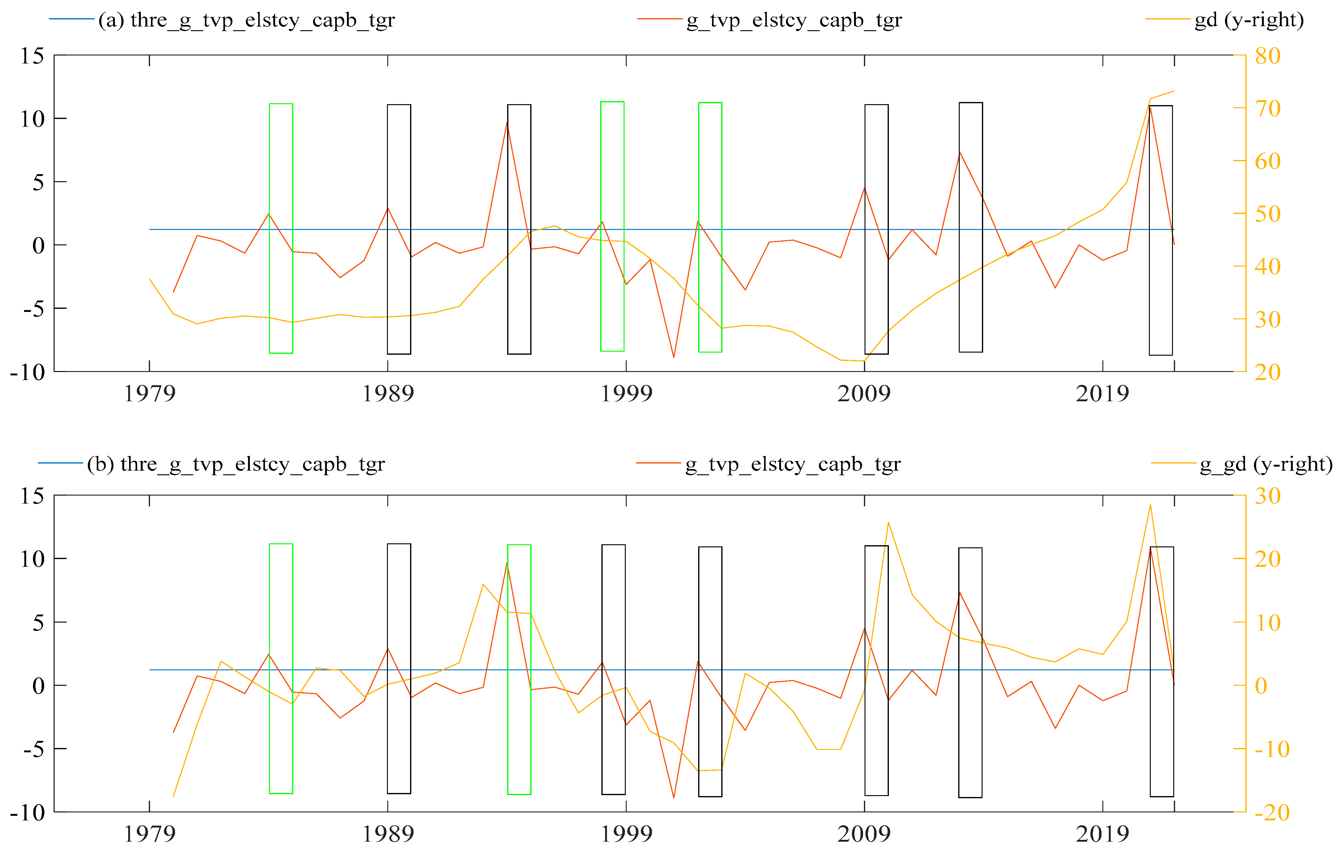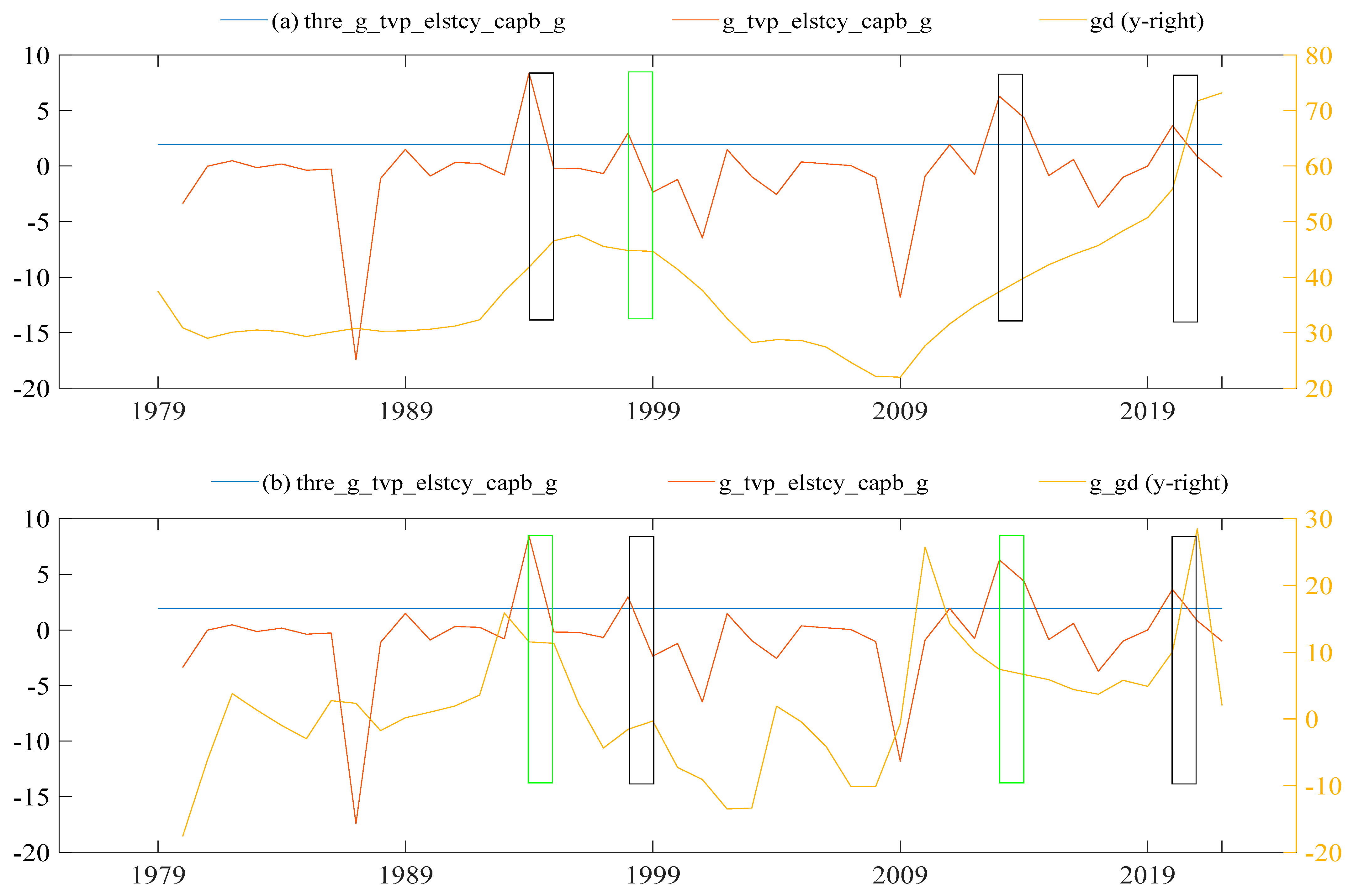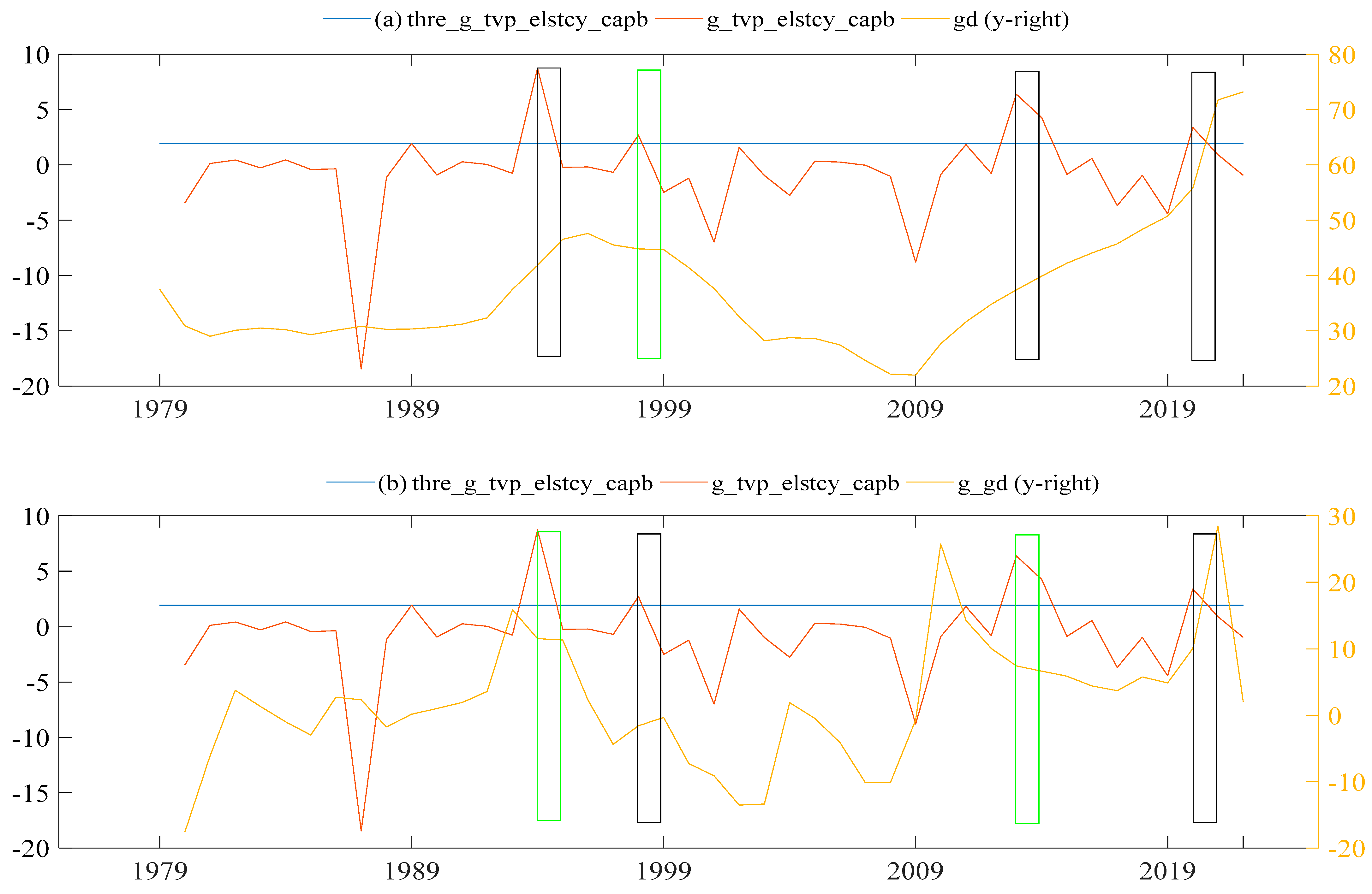Buthelezi and Nyatanga (2023), investigated the time-varying elasticity of cyclically adjusted primary balance and the effect of fiscal consolidation on domestic government debt in south Africa. Using the time-varying parameter vector autoregression (TVP-VAR) it was found that CAPB with time-varying parameters better captures the fiscal consolidation that constant elasticity of the CAPB It was found that the shock of macroeconomic uncertainty harms economic growth. Georgantas et al. (2023) highlight the importance of timing for fiscal policy adjustments. The authors argue that adjustments based on spending that are made during recessions, times of tight money, or when the debt-to-income ratio is higher than 80% are counterproductive. During recessions, cutting government spending can have negative effects on economic growth and job creation. This is because government spending helps to stimulate demand and boost economic activity. Similarly, during times of tight money, cutting government spending can lead to a further contraction in credit markets and reduce private investment. Additionally, when the debt-to-income ratio is high, cutting government spending can lead to a vicious cycle of lower growth, lower tax revenue, and higher debt levels. This is because lower government spending can lead to lower economic growth, which in turn reduces tax revenue and increases the debt-to-income ratio. On the other hand, fiscal consolidations initiated during expansions, in low-debt nations, during times of loose monetary conditions, and in open economies can be expansionary and result in a more pronounced fall in the debt ratio. During expansions, cutting government spending can help to reduce inflationary pressures and prevent overheating in the economy. In low-debt nations, cutting government spending can lead to increased confidence among investors and reduce the risk of a debt crisis. During loose monetary conditions, cutting government spending can offset the inflationary effects of easy monetary policy. Buthelezi (2023a) investigated the macroeconomic uncertainty on economic growth in the presence of fiscal consolidation in South Africa from 1994 to 2022. It was found that macroeconomic uncertainty’s negative impact on economic growth is reduced when there is an adoption of fiscal consolidation. Buthelezi (2023b) investigated the impact of government expenditure on economic growth in different states in South Africa. It was found that government expenditure increase economics growth. However, the study was silent on the role of fiscal consolidation on economic growth in South Africa. Nevertheless, this study suggests that there are times in the economy when fiscal consolidation my not the relevant. This is back positive effect of an increase in government expenditure on economic growth, while fiscal consolidation advocates for a decrease in government expenditure.

3. Methodology

This paper uses quantitative analysis to the threshold of the CAPB, fiscal consolidation episodes impact of government debt in South Africa from 1979 to 2022. The theoretical framework of the fiscal deficit is used. The fiscal deficit is a key indicator of a government’s fiscal position and refers to the amount by which government spending exceeds revenue in each period. The theoretical framework of the fiscal deficit is based on the idea that sustained deficits can have significant negative consequences for an economy, including inflation, debt accumulation, and crowding out of private investment. One of the key theoretical frameworks for understanding the fiscal deficit is the Keynesian model of macroeconomics. According to this model, government spending can play a crucial role in stimulating economic growth, particularly during periods of economic downturns. The model that is used in this paper is the threshold autoregressive regime (TAR) model. The TAR model allows for the identification of specific thresholds in the data that signal changes in the relationship between the CAPB and fiscal consolidation. The TAR model can be particularly useful in identifying nonlinearities in the data, which may not be captured by linear models (Chen et al. 2012). Another econometric tool used in the paper is the first-order derivative. This measures the rate of change of the CAPB over time and helps identify turning points in the data. By identifying these turning points, the model can help to pinpoint the exact threshold values that are associated with fiscal consolidation episodes (Chakrabarti et al. 2021). Finally, the paper also employs dummy variables, which are binary indicators that take the value of 1 if a particular event or condition is present and 0 otherwise. In this case, the dummy variables are used to capture the effect of specific fiscal consolidation episodes on the CAPB. By isolating the effect of these episodes on the CAPB, the model can estimate the threshold values that are associated with these episodes more accurately (Agnello and Sousa 2014). Overall, the combination of TAR, first-order derivative, and dummy variable models used in the paper provides a rigorous and comprehensive analysis of the relationship between CAPB and fiscal consolidation in South Africa. By identifying the threshold values that are associated with these episodes, the paper offers valuable insights into the underlying dynamics of fiscal policy in the country, which can inform policy decisions and contribute to ongoing efforts to achieve greater fiscal sustainability.

The economic variables used are $DG$ domestic government debt, $G$ government expenditure, $TGR$ total government revenue, $g\_tvp\_elstcy\_CAPB\_tgr$ growth rate time-varying CAPB for total government revenue $g\_tvp\_elstcy\_CAPB\_g$ growth rate time-varying CAPB for government expenditure $g\_tvp\_elstcy\_CAPB$ growth rate time-varying CAPB, $tvp\_elstcy\_CAPB\_tgr$ which is the time-varying CAPB for total government revenue, $tvp\_elstcyCAPB\_g$ which is time-varying CAPB for government expenditure and that $tvp\_elstcy\_CAPB$ is time-varying CAPB. The economic variables are sourced from the South African Reserve Bank, Department of National Treasury, South African Revenue Service, World Bank: World development indicators, and International Monetary Fund.

3.1. The Theoretical Framework of Fiscal Deficit

The paper uses the theoretical framework of the fiscal deficit. The fiscal deficit is the negative difference between the government’s total revenue and total government expenditures (Keynes 1937). The framework of the fiscal deficit is presented in Equation (7).

$$\begin{gathered} {GDDFCY}_t={\mathrm{G}}_t-\left(R_t+{GD}_t\right) \\ =G_t-R_t-{GD}_t \end{gathered}$$

(7)

where $GDDFC{Y}_t$ is the government deficit, $R_t$ is the revenue received by the government and the others are as defined above. The paper presents the theoretical framework of the fiscal deficit in Equation (7), concerning ${GD}_t$ domestic government debt, as shown in Equation (8).

$${GD}_t=G_t-R_t{-GDDFCY}_t$$

(8)

Equation (8) represents the ${GD}_t$ domestic government debt. In the effort to investigate the threshold of fiscal consolidation on domestic government debt, Equation (8) has attractive properties. The empirical work of this paper extends the theoretical framework by imposing fiscal consolidation variables $X_t$, as shown in Equation (9).

$${GD}_t=G_t-R_t{-GDDFCY}_t\pm X_t$$

(9)

where $X_t$ is a vector of each economic variable representing fiscal consolidation. These economic variables are $tvp\_elstcy\_CAPB\_tgr$, which is the time-varying CAPB for total government revenue, $tvp\_elstcy\_CAPB\_g$, which is the time-varying CAPB for government expenditure, and $tvp\_elstcy\_CAPB$ is the time-varying CAPB. The extension of the theoretical framework assists in finding a threshold of the CAPB that can be attributed to fiscal consolidation episodes.

3.2. Model Specification

The model that is used in this paper is the threshold autoregressive regime (TAR) model. The TAR is widely used in time series analysis to flexibly process changes over time. Other scholars have used TAR to analyze fiscal consolidation (Iqbal et al. 2017; Ramos-Herrera and Sosvilla-Rivero 2020). The TAR is effectively used to find the effect (one set of coefficients) up to the threshold and another effect (another set of coefficients) beyond it (Hansen 2000). These properties of the TAR model are attractive, as this paper seeks to investigate whether the threshold of CAPB can be attributed to fiscal consolidation. Moreover, the threshold autoregressive regime model allows for an effect beyond the threshold (Hansen 2000). This means that this paper can also ascertain the effect of fiscal consolidation episodes. The TAR model can move from different states of the economy. This provides attractive properties, as the empirical work of this study can find the threshold present with the different states of domestic government debt. A threshold variable that is above or below a threshold value identified may have numerous thresholds, and one can either specify a known number or let the Bayesian Information Criterion (BIC), Akaike Information Criterion (AIC), or Hannan–Quinn Information Criterion (HQC) find that number for you (HQIC) (Iqbal et al. 2017; Ramos-Herrera and Sosvilla-Rivero 2020). The TAR model of (Hansen 2000) is shown in Equations (10) and (11).

$$y_t={\theta }_1^{\prime }{x}_t+{\mathsf{ϵ}}_{1t} if q_t\le \gamma$$

(10)

$$y_t={\theta }_2^{\prime }{x}_t+{ϵ}_{2t} if q_t\le \gamma$$

(11)

where $y_t$ is the dependent variable, $x_t$ is the independent variable, $q_t$ is the threshold variable, ${ϵ}_{1t}$ is the error term, and $\gamma$ is the threshold value. Equation (10) shows that the threshold variable is smaller than the threshold value. In Equation (11), the threshold variable is greater than the threshold value. The model assumes a dummy variable $I_t\left(\gamma \right)=q_t\le \gamma$, which is an indicator function. The dummy variable can also be presented as $q_t\le \gamma$ then, $I=1$ or otherwise $I=0$. If we let $x_t\left(\gamma \right)$ = $x_t{I}_t\left(\gamma \right)$, this will result in rewriting Equations (10) and (11) as Equation (12).

$$y_t={\theta }_1^{\prime }{x}_t+{\rho }^{\prime }{x}_t\left(\gamma \right)+{ϵ}_{1t} and {ϵ}_{1t}~iid0,{\sigma }_t^2$$

(12)

where $\theta ={\theta }_2$ ρ = ${\theta }_1$ − ${\theta }_2$, and the error term ${\mathsf{ϵ}}_{1t,}{\mathsf{ϵ}}_{2t}$, where $\theta ,\rho$ and $\gamma$ are the parameters to be estimated. The parameters arrive at the sum of squared errors and can be presented in Equation (13).

$$S_1\left(\mathsf{\gamma }\right)={\widehat{\mathsf{ϵ}}}_t^{\prime }{\left(\mathsf{\gamma }\right)}^{\prime }{\widehat{\mathsf{ϵ}}}_t\left(\mathsf{\gamma }\right)$$

(13)

The optimum threshold value is given by Equation (14).

$$\widehat{\mathsf{\gamma }}=arg min{S}_1\mathsf{\gamma }$$

(14)

The variance of the residual is given by Equation (15).

$${\widehat{\mathsf{\sigma }}}^2 = \frac{1}{T}{\widehat{\mathsf{ϵ}}}_t^{\prime }{\widehat{\mathsf{ϵ}}}_t=\frac{1}{T}{S}_1\left(\widehat{\mathsf{\gamma }}\right)$$

(15)

Once $\widehat{\mathsf{\gamma }}$ is obtained, the vectors of the slope coefficient to be estimated are $\widehat{\theta }$ = $\widehat{\theta }$($\widehat{\mathsf{\gamma }}$) and $\widehat{\rho }$ = $\widehat{\rho }$ ($\widehat{\mathsf{\gamma }}$). The theoretical framework that is outlined in Equation (9) is applied in the threshold autoregressive regime model outlined in Equations (17a), as well as (18a) and the estimation of Equations (16)–(18).

$$gd=\left\{\begin{array}{c}{\mathsf{\beta }}_{10}+{\mathsf{\beta }}_{11}{g}_t+{\mathsf{\beta }}_{12}tg{r}_t+{\mathsf{\beta }}_{13}tvp\_elstcy\_CAPB\_tg{r}_t\\ {\mathsf{\beta }}_{20}+{\mathsf{\beta }}_{21}{g}_t+{\mathsf{\beta }}_{22}{tgr}_t+{\mathsf{\beta }}_{23}tvp\_elstcy\_CAPB\_tg{r}_t+{\mathsf{ϵ}}_t^{*}\end{array}\right.$$

(16)

$$gd=\left\{\begin{array}{c}{tvp\_elstcy\_CAPB\_tgr}_t \left[q_t\le \gamma \right]\\ {tvp\_elstcy\_CAPB\_tgr}_t+{ϵ}_t^{*} \left[q_t>\gamma \right]\end{array}\right.$$

(16a)

$$gd=\left\{\begin{array}{c}{\mathsf{\beta }}_{10}+{\mathsf{\beta }}_{11}{g}_t+{\mathsf{\beta }}_{12}tg{r}_t+{\beta }_{13}tvp\_elstcy\_CAPB\_g_t\\ {\mathsf{\beta }}_{20}+{\mathsf{\beta }}_{21}{g}_t+{\mathsf{\beta }}_{22}{tgr}_t+{\beta }_{23}tvp\_elstcy\_CAPB\_g_t+{ϵ}_t^{*}\end{array}\right.$$

(17)

$$gd=\left\{\begin{array}{c}{tvp\_elstcy\_CAPB\_g}_t \left[q_t\le \gamma \right]\\ {tvp\_elstcy\_CAPB\_g}_t+{ϵ}_t^{*} \left[q_t>\gamma \right]\end{array}\right.$$

(17a)

$$gd=\left\{\begin{array}{c}{\mathsf{\beta }}_{10}+{\mathsf{\beta }}_{11}{g}_t+{\mathsf{\beta }}_{12}tg{r}_t+{\beta }_{13}{tvp\_elstcy\_CAPB}_t\\ {\mathsf{\beta }}_{20}+{\mathsf{\beta }}_{21}{g}_t+{\mathsf{\beta }}_{22}{tgr}_t+{\beta }_{23}{tvp\_elstcy\_CAPB}_t+{ϵ}_t^{*}\end{array}\right.$$

(18)

$$gd=\left\{\begin{array}{c}{tvp\_elstcy\_CAPB}_t \left[q_t\le \gamma \right]\\ {tvp\_elstcy\_CAPB}_t+{ϵ}_t^{*} \left[q_t>\gamma \right]\end{array}\right.$$

(18a)

The threshold value $\gamma$ is found by estimating Equations (16a), (17a) and (18a) from a minimum of a sum of squared errors in a reorder threshold variable. The threshold will present $tvp\_elstcy\_CAPB\_tgr,tvp\_elstcy\_CAPB\_g$ and $tvp\_elstcy\_CAPB$, which can be attributed to fiscal consolidation, as outlined by (Alesina and Ardagna 2013; Yang et al. 2015). To check the stationarity in the time series to ensure that there is a constant mean in the time series. This is carried out to filter out trends and seasonality that may affect the estimation Baum and Otero (2021). The unit root test used in the paper is the augmented Dickey-Fuller test (ADF). The generally estimated Equation (19) is as follows:

$$\mathsf{\Delta }{y}_t={\beta }_0+{\beta }_1{X}_{t-1}+\sum _{t=1}^n\beta X_i+{\eta }_i+e_t$$

(19)

where $y_t$ is a time series, $t$ is the linear time series trend, Δ is the first difference, ${\beta }_0$ is the constant and ${\eta }_i$ is an optimum number of lags in the dependent variable.

4. Results

Table 3. Descriptive statistics of the data sourced and estimated.

Variable	Obs	Mean	Std. Dev.	Min	Max	Skewness	Kurtosis	Shapiro–Wilk
$GD$	44	37.2268	11.2063	21.99	73.18	0.000	0.69	0.548
$G\_GD$	43	0.01971	0.09279	−0.176	0.28484	0.032	0.40	0.895
$G$	44	27.9489	3.00313	23.3	37.5	0.000	0.08	0.901
$TGR$	44	14.32779	8.754365	−5.2537	36.8419	0.024	0.20	0.533
$GDFCY$	44	−3.3545	1.92178	−7.2	0.7	0.001	0.07	0.951
$tvp\_elstcy\_CAPB\_tgr$	44	−1.35659	12.22918	−47.3	49.72	0.317	0.67	0.928
$tvp\_elstcy\_CAPB\_g$	44	5.259546	45.5113	−247.4	67.85	0.001	0.32	0.901
$tvp\_elstcy\_CAPB$	44	6.616136	56.26286	−297.13	115.15	0.000	0.05	0.908

The authors’ processing of the table above.

shows descriptive statistics of economic variables from 1979 to 2022 used in this study. The second part of Table 3 reflects the descriptive statistics of the data that are calculated and estimated. The $GD$ is found to have a mean of 37.22%. The $G\_GD$ is found to have a mean value of 27.94%. The level of $G$ is found to have an average of 27.94% between 1979 and 2022. Total government revenue, $TGR$ is found to have a growth rate mean of 14.32%. The economic variables that are considered in the paper are all positively skewed. The kurtosis reflects an atheoretical measure of the normal distribution with the economic variables that have the highest value being the $GD$ total domestic government debt will have a value of 0.69. This value suggests that the $GD$ total domestic government debt is leptokurtic, that is, it was highly peaked with a very thin tail. The Shapiro–Wilk probability p values are higher than 0.05%; as such, we fail to reject that there is no normal distribution among economic variables. The $tvp\_elstcy\_CAPB\_tgr$ time-varying CAPB for total government revenue, $tvp\_elstcy\_CAPB\_g$ time-varying CAPB for government expenditure, and the $tvp\_elstcy\_CAPB$ time-varying CAPB are found to have mean values of −1.35%, 5.25%, and 6.61%, respectively.

Table 4. Dickey-Fuller test.

Variables		Dickey-Fuller Test for Unit Root
		Test	1%	5%	10%
$D.GD$	Z(t)	−9.517	−3.535	−2.904	−2.587
$G\_GD$	Z(t)	−3.902	−3.634	−2.952	−2.610
$D.GDFCY$	Z(t)	−7.018	−3.634	−2.952	−2.610
$D.G$	Z(t)	−9.406	−3.736	−2.994	−2.628
$D.TGR$	Z(t)	−9.221	−3.634	−2.952	−2.610
$thre\_g\_tvp\_elstcy\_CAPB\_tgr$	Z(t)	−5.857	−3.628	−2.950	−2.608
$thre\_g\_tvp\_elstcy\_CAPB\_g$	Z(t)	−6.414	−3.628	−2.950	−2.608
$thre\_g\_tvp\_elstcy\_CAPB$	Z(t)	−6.481	−3.634	−2.952	−2.610

The authors’ processing of the table above.

shows the stationarity test results of the Dickey-Fuller. The test results show that the unit root null hypothesis could not be rejected in levels but was rejected in first differences at 1%. This is because all t-test values of economic variables of $D.GD,GGD,D.GDFCY,D.G,$ and $D.TGR$ are greater than the first differences at 1%. As such, it is concluded that the economic variables of $D.GD,D.G,D.RD,$ and $D.TG$ are stationary at first differences. The $tvp\_elstcy\_CAPB\_tgr$ time-varying CAPB for total government revenue, $tvp\_elstcy\_CAPB\_g$ time-varying CAPB for government expenditure, and the $tvp\_elstcy\_CAPB$ time-varying CAPB are found to be stationary at $I\left(0\right)$.

Table 5. Threshold autoregressive regime model.

Estimation	1	2	3
Variables	$DG$	$DG$	$DG$
$Region1$
$\_Cons$	36.22 **	34.07 **	34.75 **
	(0.000)	(0.000)	(0.000)
$Region2$
$\_Cons$	45.89 **	45.75 **	45.75 ***
	(0.000)	(0.000)	(0.000)
$thre\_g\_tvp\_elstcy\_CAPB\_tgr$	2.8962
$thre\_g\_tvp\_elstcy\_CAPB\_g$		0.4755
$thre\_g\_tvp\_elstcy\_CAPB$			0.4418
$AIC$	213.9803	213.1298	214.8339
$BIC$	221.2665	220.2665	221.9707
$HQIC$	216.6269	215.7764	217.4806
$N$	44	44	44
t statistics in parentheses, * p < 0.05, ** p < 0.01, *** p < 0.001, Akaike information criterion (AIC), Bayesian information criterion (BIC) and Hannan-Quinn information criterion (HQC) is a measure of the goodness of fit of a statistical model.
Estimation 1 is related to $gd=\left\{\begin{array}{c}{tvp\_elstcy\_CAPB\_tgr}_t \left[q_t\le \gamma \right]\\ {tvp\_elstcy\_CAPB\_tgr}_t+{ϵ}_t^{*} \left[q_t>\gamma \right]\end{array}\right.$
Estimation 2 is related to $gd=\left\{\begin{array}{c}{tvp\_elstcy\_CAPB\_g}_t \left[q_t\le \gamma \right]\\ {tvp\_elstcy\_CAPB\_g}_t+{ϵ}_t^{*} \left[q_t>\gamma \right]\end{array}\right.$
Estimation 3 is related to $gd=\left\{\begin{array}{c}{tvp\_elstcy\_CAPB}_t \left[q_t\le \gamma \right]\\ {tvp\_elstcy\_CAPB}_t+{ϵ}_t^{*} \left[q_t>\gamma \right]\end{array}\right.$

The authors’ processing of the table above.

reflects the threshold autoregressive regime model from 1979 to 2022. It is found that $GD$ has a mean value of 36.22% in regime 1, which is 1.22% lower than the mean rate of the sample, which is 37.22%.

Regime 2 $GD$ has a mean value of 45.89%, which is a regime reflecting the unstable level of domestic government debt. The rate of 45.89% is 8.67% higher than the sample means, and the rate of domestic government debt is 37.22%. It is critical for South Africa to manage its domestic government debt since failing to do so might result in a major rise in risk and a decrease in the effectiveness of the market for government securities. As a result, the government must develop and implements a clear and efficient plan for controlling its debt levels. The creation of a legal framework outlining the government’s ability to borrow, issue, invest in, and trade additional debt may be required in addition to the adoption of such a strategy. This framework would need to be created to lower domestic government debt and ensure that all borrowing and investing operations are conducted responsibly and openly. An effective market for government securities is essential for the health of the economy since it gives investors a secure and trustworthy investment opportunity while also enabling the government to receive money at fair rates. South Africa can support the upkeep of a steady and functional market for government securities by properly controlling its debt levels and putting in place a regulatory framework that encourages responsible borrowing and investment practices. In the end, the success of any plan for controlling government debt in South Africa would depend on several variables, including the state of the economy, political stability, and the capacity of the government to make tough choices and put them into action. However, South Africa can contribute to ensuring its long-term economic stability and prosperity by prioritizing this issue and adopting proactive measures to address it.

Table 6. Threshold autoregressive regime model with a focus on thresholds.

Estimation	1	2	3
Variables	$DG$	$DG$	$DG$
$\mathrm{R}\mathrm{e}\mathrm{g}\mathrm{i}\mathrm{m}\mathrm{e}1$
$G$	2.257 ***	1.873 ***	1.971 ***
	(0.000)	(-0.001)	(0.000)
$TGR$	−0.451 **	−0.312	−0.358 *
	(−0.008)	(−0.059)	(−0.026)
$\_Cons$	−14.82	−11.59	−13.31
	(−0.347)	(−0.443)	(−0.379)
$\mathrm{R}\mathrm{e}\mathrm{g}\mathrm{i}\mathrm{m}\mathrm{e}2$
$G$	2.024 ***	1.475 ***	1.018 ***
	(0.000)	(−0.000)	(0.000)
$TGR$	−0.3001 **	−0.256	−0.253 *
	(−0.000)	(−0.012)	(−0.025)
$\_Cons$	−19.69	−1.211	−3.503
	(−0.221)	(−0.94)	(−0.827)
$thre\_g\_tvp\_elstcy\_CAPB\_tgr$	−1.2168
$thre\_g\_tvp\_elstcy\_CAPB\_g$		1.9182
$thre\_g\_tvp\_elstcy\_CAPB$			1.927
$AIC$	213.9803	213.1298	214.8339
$BIC$	221.2665	220.2665	221.9707
$HQIC$	216.6269	215.7764	217.4806
$N$	44	44	44
t statistics in parentheses, * p < 0.05, ** p < 0.01, *** p < 0.001, Akaike information criterion (AIC), Bayesian information criterion (BIC) and Hannan-Quinn information criterion (HQC) is a measure of the goodness of fit of a statistical model.
Estimation 1 is related to $gd=\left\{\begin{array}{c}{\mathsf{\beta }}_{10}+{\mathsf{\beta }}_{11}{g}_t+{\mathsf{\beta }}_{12}tg{r}_t+{\mathsf{\beta }}_{13}tvp\_elstcy\_CAPB\_tg{r}_t\\ {\mathsf{\beta }}_{20}+{\mathsf{\beta }}_{21}{g}_t+{\mathsf{\beta }}_{22}{tgr}_t+{\mathsf{\beta }}_{23}tvp\_elstcy\_CAPB\_tg{r}_t+{\mathsf{ϵ}}_t^{*}\end{array}\right.$
Estimation 2 is related to $gd=\left\{\begin{array}{c}{\mathsf{\beta }}_{10}+{\mathsf{\beta }}_{11}{g}_t+{\mathsf{\beta }}_{12}tg{r}_t+{\mathsf{\beta }}_{13}tvp\_elstcy\_CAPB\_g_t\\ {\mathsf{\beta }}_{20}+{\mathsf{\beta }}_{21}{g}_t+{\mathsf{\beta }}_{22}{tgr}_t+{\mathsf{\beta }}_{23}tvp\_elstcy\_CAPB\_g_t+{\mathsf{ϵ}}_t^{*}\end{array}\right.$
Estimation 3 is related to $gd=\left\{\begin{array}{c}{\mathsf{\beta }}_{10}+{\mathsf{\beta }}_{11}{g}_t+{\mathsf{\beta }}_{12}tg{r}_t+{\beta }_{13}{tvp\_elstcy\_CAPB}_t\\ {\mathsf{\beta }}_{20}+{\mathsf{\beta }}_{21}{g}_t+{\mathsf{\beta }}_{22}{tgr}_t+{\beta }_{23}{tvp\_elstcy\_CAPB}_t+{ϵ}_t^{*}\end{array}\right.$

, estimation 1, shows that $G$ has a positive impact on $DG$. These results suggest that a 1% increase in $G$ would result in a 2.257% increase in $DG$, all else being equal. These results agree with the classical school of thought rationale that less need for government intervention is needed in the economy (Mankiw 2019). $TGR$ is found to have a negative relationship with, $DG$ and a 1% increase in total government revenue will result in a 0.451% decrease in domestic government debt. These results are similar to those of Gupta et al. (2005), McDermott and Wescott (1996), and Zaghini (2001). The $thre\_g\_tvpelstcy\_CAPB\_tgr$ is found to have a threshold of negative 1.2168%, which indicates that the growth rate with time-varying elasticity of the cyclical adjusted primary balance for total government revenue that is above 1.2168% could be attributed to fiscal consolidation that is achieved using tax increases.

This threshold is lower by 0.2832% from the threshold improvement in the CAPB advocated by Arestis et al. (2018); Blanchard (1990); and McDermott and Wescott (1996) among other scholars. However, the negative sign on the threshold of $thre\_g\_tvpelstcy\_CAPB\_tgr$ outlines that fiscal consolidation of tax increases can result in a reduction in $DG$. These results are not in line with the results of Gupta et al. (2005); McDermott and Wescott (1996); and Zaghini (2001), among others, that point to tax fiscal consolidation influencing the reduction of government debt. Moreover, the results suggest that the South African fiscal authorities should look at different tax brackets to apply fiscal consolidation that may reduce $DG$.

The $thre\_g\_tvp\_elstcy\_CAPB\_g$ is found to have a threshold value of 1.9182%, outlining that it is above 1.9182%, which will identify the fiscal consolidation episode that is undertaken through the government expenditure cut. This threshold is higher by 0.418% than that of Arestis et al. (2018), which is identified through the increase in the CAPB. The $thre\_g\_tvp\_elstcy\_CAPB$ growth rate time-varying elasticity cyclical adjusted primary balance for both fiscal consolidations achieved through government expenditure cuts and a tax increase has a threshold value of 1.9270%. This threshold is higher by 0.427% than that of Arestis et al. (2018); Blanchard (1990); McDermott and Wescott (1996), which is identified through the increase in the CAPB of 1.5%. The threshold has a positive value of 1.9270%, suggesting that fiscal consolidation is achieved through government expenditure cuts and tax increases. If adopted simultaneously, this will increase domestic government debt. Therefore, the adoption of fiscal consolidation using both tax increases and government expenditure cuts is undesirable in South Africa, as it will increase domestic government debt. This result is contrary to that of Glavaški and Beker-Pucar (2020), who found that the CAPB has a positive impact on economic growth, and the primary budget balance in GDP increases by 1%.

Figure 1, graph a, shows $thre\_g\_tvpelstcy\_CAPB\_tgr$ with a threshold value of 1.2168%. Given this threshold, there are eight fiscal consolidation episodes in 1984, 1989, 1994, 1998, 2002, 2013, and 2021. The success of fiscal consolidation through tax revenue is defined by the reduction in $GD$. There were three successful fiscal consolidations undertaken through government revenue in 1984, 2002, and 2013. The years 1989, 1994, 2002, 2013, and 2021 reflect five fiscal consolidation episodes that are unsuccessful, given that after these episodes, domestic government debt increased. The paper looks at the success of fiscal consolidation in the context of how fast it is in reducing domestic government debt. As such, the $G\_GD$ growth rates of domestic government debt are considered. Figure 1, graph b, shows that there are three out of eight fiscal consolidation episodes were successful in reducing $G\_GD$. These results suggest a 37.5% chance that fiscal consolidation undertaken through government revenue would reduce domestic debt and reduce the growth in the domestic government debt rate. There is a 62.5% chance that fiscal consolidation undertaken through government revenue may not be successful in reducing domestic government debt and the growth rate of domestic government debt.

Figure 2, graph a, shows that $thre\_g\_tvpelstcy\_CAPB\_g$ is found to have a threshold value of 1.9182%, which may indicate the point at which fiscal consolidation can effectively reduce government debt. This threshold value could be based on various factors, such as the size of the government debt, the level of economic growth, and the effectiveness of fiscal consolidation policies. The analysis has identified four episodes of fiscal consolidation in 1994, 1998, 2013, and 2020, which could be specific to the country or regime under consideration. The results suggest that only two of these episodes, in 1994 and 2013, led to a reduction in $G\_GD$, which is a measure of government debt relative to the size of the economy. This could indicate that fiscal consolidation policies implemented during these episodes were effective in reducing government debt. Based on these findings, the analysis suggests that there is a 25% chance that government expenditure reduction through fiscal consolidation can reduce domestic government debt. This suggests that fiscal consolidation policies that focus on reducing government spending may not always lead to a reduction in government debt, and other factors such as economic growth and revenue generation may also play a role.

Additionally, the analysis suggests a 50% chance that fiscal consolidation can lead to a reduction in the growth rate of domestic government debt. This indicates that fiscal consolidation policies may not only reduce government debt but also slow its growth rate. However, it is important to note that the effectiveness of fiscal consolidation policies can depend on various factors such as the size and structure of the economy, the level of public debt, the political environment, and the implementation of policy measures. Therefore, the implication of the results is the importance of fiscal consolidation in reducing government debt and its potential impact on economic growth and stability. However, it also suggests that the effectiveness of fiscal consolidation policies can vary depending on several factors and that further research is required to fully understand its impact.

Figure 3, graph a, shows that $thre\_g\_tvpelstcy\_CAPB$ is found to have four fiscal consolidation episodes from the threshold of 1.9270% in 1994, 1998 and 2013 and 2020. The results also suggest a 50% chance that fiscal consolidation episodes will reduce the $G$ growth rate of domestic government debt. Table 3 shows the summary of fiscal consolidation episodes in this study. There is an indication that out of eight fiscal consolidations $thre\_g\_tvp\_elstcy\_CAPB\_tgr$, there are three that are successful, which is 37.50%, and these can be deemed effective in reducing domestic government debt. The $thre\_gtvp\_elstcy\_CAPB\_g$ there is a 25% chance that after fiscal consolidation episodes will reduce domestic government debt. The $thre\_g\_tvp\_elstcy\_CAPB$ there is a 25% chance that after fiscal consolidation episodes will reduce domestic government debt.

From the analysis of the above three figures, it can be observed that fiscal consolidation episodes undertaken through government revenue have a 37.5% chance of being successful in reducing domestic government debt and the growth rate of such debt, while there is a 62.5% chance of such episodes being unsuccessful. On the other hand, fiscal consolidation episodes undertaken through government expenditure have a 25% chance of being successful in reducing domestic government debt and a 50% chance of reducing the growth rate of such debt. The results suggest that fiscal consolidation episodes undertaken through government revenue are more likely to be successful in reducing domestic government debt and its growth rate compared to those undertaken through government expenditure. However, the success rate is still relatively low, indicating the need for further research and analysis in this area. It is recommended that policymakers consider undertaking fiscal consolidation through government revenue as a preferred option. However, given the low success rate, it is also important to explore other policy options for reducing domestic government debt, such as increasing economic growth, improving tax collection, reducing nonessential spending, and addressing structural issues in the economy. In addition, policymakers should carefully consider the timing and pace of fiscal consolidation episodes, as well as the specific policy measures used, to increase the chances of success. It is also important to communicate the rationale and objectives of fiscal consolidation efforts to the public and stakeholders to ensure support and cooperation.

Table 7. Summary of fiscal consolidation episodes and that of this paper.

Author	Definition	EB	TB	TE	TS	% S
Alesina and Perotti (1995)	Threshold of 1.5% CAPB	59	60	119	66	55.46%
(McDermott and Wescott 1996)	Threshold of 1.5% CAPB	34	74	108	43	39.81%
Alesina et al. (1998)	Threshold of 2% CAPB	23	28	51	19	37.25%
Zaghini (2001)	Threshold of 1.6% or 1.4% of CAPB	52	48	100	52	52.00%
Duperrut (1998)	Threshold of 1.6% or 1.4% of CAPB			9	2	22.22%
Afonso and Silva Leal (2019)	Threshold of 1.5% CAPB			51		18.61%
Quaresma (2021)	Threshold of 1.5% CAPB and the narrative approach	76	60	136	36	26.47%
Wiese et al. (2018)	Threshold of 1.5% CAPB and the narrative approach	42	58	110	50	45.45%
Nunes (2019)		61	52	113	25	22.12%
Agnello et al. (2019)	Threshold of 1.5% CAPB and the narrative approach			51	15	29.41%
Afonso and Silva Leal (2022)	Threshold of 1.5% CAPB and the narrative approach	81	98	179	45	25.13%
This paper	$thre\_g\_tvp\_elstcy\_CAPB\_tgr$ 1.2168%		8	8	3	37.50%
	$thre\_g\_tvp\_elstcy\_CAPB\_g$ 1.9182%	4		4	1	25.00%
	$thre\_g\_tvp\_elstcy\_CAPB$ 1.9270%			4	1	25.00%

Note: EB reflects the expenditure base fiscal consolidation, TB tax-based fiscal consolidation, TE total expenditure-based, TS total fiscal consolidation success and % Total fiscal consolidation success as a percentage. The authors’ processing of the table above.

shows the summary of fiscal consolidation episodes and that of this paper, it is noted that the threshold found in this paper is different to that provided by the literature.

5. Discussion and Recommendation

The paper investigates the threshold of the CAPB that can be attributed to fiscal consolidation episodes in South Africa. The identified problem is that there is no specific rate or threshold as to how much improvement in CAPB can be attributed to fiscal consolidation episodes. The literature defined fiscal consolidation episodes only by referring to large changes in the CAPB without giving an analysis of these values. The empirical work of this study bridges the gap of none explained fiscal consolidation episodes using the theoretical framework of fiscal deficit and using the threshold autoregressive regime (TAR) model. There is an indication that there is a threshold of 1.2168% for $thre\_g\_tvp\_elstcy\_capb\_tgr$ reflecting fiscal consolidation episodes achieved through tax, a threshold of 1.9182% for $thre\_g\_tvp\_elstcy\_capb\_g$ reflecting fiscal consolidation achieved through government expenditure and a threshold of 1.9270% $thre\_g\_tvp\_elstcy\_capb$ reflecting fiscal consolidation episodes achieved through using both government expenditure and tax.

Given this result, it is the view of the author that there should be an imposition of a threshold of 1.5% of the CAPB, as advocated by (Afonso 2010; Afonso et al. 2022b; Alesina and Perotti 1995, 1997; Alesina et al. 1998; Alesina and Ardagna 2010; Devries et al. 2011; Giavazzi and Pagano 1995; Guajardo et al. 2014; Romer and Romer 2010; Yang et al. 2015) Barrios et al. (2010), among others. This stands only on the institution that the rate of 1.5% is effective and large enough to reflect fiscal consolidation episodes that are not associated with the cyclical movement. As such, the threshold of 1.5% can be used to identify discretionary actions of fiscal authorities that are equivalent to fiscal consolidation episodes that may not hold. This view of the author is backed by the findings of the paper, which found a $thre\_g\_tvp\_elstcy\_capb$ threshold of 1.9270%, which is 0.427% higher than that in the literature of Arestis et al. (2018); Blanchard (1990); and McDermott and Wescott (1996), among others. Moreover, it is the view of the author that there may be a fallacy of composition that the threshold of 1.5% may be used in studies that are regionally based as well as those that are based at the country level. The result of the paper suggests that a country-based threshold analysis is needed in the effort to find fiscal consolidation episodes.

It is the author’s view that the paper is critical and adds to the body of knowledge by further dis-aggregating the threshold of the CAPB by including the $thre\_g\_tvp\_elstcy\_capb\_tgr$ and $thre\_g\_tvp\_elstcy\_capb\_g$ which literature is silent on. The literature uses tax and government expenditure as economic variables for the CAPB or the assessment of each, regarding the impact of these two economic variables on domestic government debt. To this end, it is to the best of the author’s knowledge that tax and government expenditure has not been used as thresholds that can be attributed to fiscal consolidation and calculated rather than imposed. The paper reflects that there are four fiscal consolidations of $thre\_g\_tvp\_elstcy\_capb$, and there is one that is successful, which is 25.00%. It is the author’s view that fiscal consolidation in South Africa may not be effective in the effort to reduce domestic government debt. The results suggest that 75.00% of synchronized fiscal consolidation episodes are achieved with the use of both government expenditure cuts and a tax increase that is not effective when using domestic government debt. As such, the contraction-expansionary-fiscal policy advocated in the non-Keynesian approach (Mankiw 2020) does not hold in the South African economy.

The paper reflects that there is a 25% and 37.50% chance that the $thre\_g\_tvp\_elstcy\_capb\_g$ and $thre\_g\_tvp\_elstcy\_capb\_tgr$ fiscal consolidation episodes, respectively, will result in the successful reduction of domestic government debt in South Africa. It is the author’s view that this result has policy implications and that the fiscal authority must be taken into consideration since the results indicate that fiscal consolidations based on tax increases are more often connected with expansionary effects and have more success in reducing domestic government debt and budget deficits in comparison with a reduction in government expenditure. This result is contrary to the literature that advocates that government expenditure cuts are better than tax increases, as outlined by Arestis et al. (2018); Blanchard (1990); and McDermott and Wescott (1996), among others. Nevertheless, fiscal authorities must consider the economic theory of the Laffer Curve (Mankiw 2020) since a tax increase with the application of fiscal consolidation could be a time when it will start to be detrimental to the economy and result in increases in domestic government debt. It is the author’s view that the disputed tax is seemingly better than the government expenditure cut. Moreover, there is a need for willingness from firms as well as South Africa’s fiscal authorities to work together in economic decisions as well as the planning of government activities. As such, with tax increases, the private sector will know what this revenue for the government will be used for and what business opportunities firms have. The fiscal authorities must consider the trade between the crowding out investment and interest tax as part of implementing fiscal consolidation since, with a tax increase with the application of fiscal consolidation, there could be a time when it will start to be detrimental to the economy and result in increases in domestic government debt. It is the author’s view that the disputed tax is seemingly better than the government expenditure cut. Moreover, there is a need for willingness from firms as well as South Africa’s fiscal authorities to work together in economic decisions as well as the planning of government activities. As such, with tax increases, the private sector will know what this revenue for the government will be used for and what business opportunities firms have. The fiscal authorities must consider the trade between crowding out investment and interest tax as part of implementing fiscal consolidation. Fiscal consolidation $threg\_tvp\_elstcy\_capb\_g$ reflects that there is 25% success in reducing domestic government debt when there is a government expenditure cut. It is the author’s view that if the government expenditure cut is implemented, it needs to be on the government categories that will not limit the administration of the government and service delivery. Fiscal authorities need to note that fiscal consolidation episodes of government expenditure cuts have a 75% chance of not being successful in domestic government debt.

The same policy is present in the four fouls. First, they adopt a country-based approach to fiscal consolidation. The paper’s finding that there are different thresholds for the cyclical adjusted primary balance (CAPB) that can be attributed to fiscal consolidation episodes suggests that fiscal authorities should tailor their fiscal targets and policies to the specific economic conditions and needs of South Africa. This would involve setting targets that are realistic and achievable, given the country’s economic growth prospects, revenue base, and expenditure needs. Second, increase government revenue. The paper finds that a threshold of 1.9182% increase in total government revenue could be attributed to fiscal consolidation episodes. This suggests that fiscal authorities could focus on increasing revenue through a range of measures such as tax reforms, expanding the tax base, and reducing tax evasion. This could help to reduce the need for spending cuts and limit the impact of fiscal consolidation on growth and social spending. Third, control government spending. The paper finds that a threshold of 1.9270% for the CAPB as a sum of both revenue and expenditure could be attributed to fiscal consolidation episodes. This suggests that fiscal authorities could focus on controlling government spending, particularly nonessential spending, to reduce the fiscal deficit and debt levels. This could involve measures such as reducing subsidies, rationalizing public sector wages, and improving public procurement processes. Lastly, boost economic growth. The paper suggests that one of the main challenges of fiscal consolidation in South Africa is the country’s low economic growth prospects. To address this, fiscal authorities could focus on implementing structural reforms that promote private sector investment, reduce red tape, and improve the business environment. This could help to boost economic growth and revenue, making fiscal consolidation easier to achieve.

6. Conclusions

The empirical work of this paper is to investigate the thresholds that reflect fiscal consolidation episodes in South Africa. Scholars have only relied on intuition in explaining the threshold of economic variables that can be attributed to fiscal consolidation. This results in different values of the fiscal consolidation threshold, which may lead to different fiscal consolidation episodes. Therefore, a country-based investigation is critical. This empirical work seeks to fill the gap in the identification of the threshold using the CAPB. As such, the economic question of this paper is what is the threshold in the CAPB that can be attributed to fiscal consolidation? What fiscal consolidation reflects success in reducing government debt? We investigated the threshold in the CAPB that can be attributed to fiscal consolidation in South Africa. The CAPB framework is used in the threshold autoregressive regime (TAR) using time series data from 1979 to 2022.

This paper aims to investigate the threshold of the cyclically adjusted primary balance (CAPB) that reflects fiscal consolidation episodes in South Africa. The current literature lacks a clear understanding of the threshold of economic variables that can be attributed to fiscal consolidation, resulting in varying values for the fiscal consolidation threshold. Therefore, this empirical work seeks to fill this gap by identifying the threshold of the CAPB using time series data from 1979 to 2022. The paper found that the threshold values for the CAPB of total government revenue increase, government expenditure cut, and the CAPB as a sum of both revenue and expenditure are −1.28168%, 1.9182%, and 1.9270%, respectively, which differ from the threshold of 1.5% suggested in the literature.

The findings of this paper offer several recommendations for policymakers in South Africa and other countries with high government debt levels. First, policymakers should conduct country-specific investigations to identify the threshold of economic variables that can be attributed to successful fiscal consolidation. Second, policymakers should prioritize tax increases as a primary tool for fiscal consolidation while being mindful of the potential negative impacts on economic growth and social welfare. Finally, policymakers should monitor the impact of their fiscal consolidation strategies on domestic government debt and its growth rate to ensure that they are effective in achieving their goals.

References

1. Afonso, António, Christiane Nickel, and Philipp C. Rother. 2006. Fiscal consolidations in the Central and Eastern European countries. Review of World Economics 142: 402–21. [Google Scholar] [CrossRef]
2. Afonso, António. 2010. Expansionary fiscal consolidations in Europe: New evidence. Applied Economics Letters 17: 105–9. [Google Scholar] [CrossRef]
3. Afonso, António, and João Tovar Jalles. 2013. Growth and productivity: The role of government debt. International Review of Economics & Finance 25: 384–407. [Google Scholar]
4. Afonso, António, and Frederico Silva Leal. 2019. Fiscal Episodes in the EMU: Elasticities and Non-Keynesian Effects. REM Working Paper 097-2019. Lisbon: Universidade de Lisboa. [Google Scholar]
5. Afonso, António, José Alves, and João Tovar Jalles. 2022a. The (non-)Keynesian effects of fiscal austerity: New evidence from a large sample. Economic Systems 46: 100981. [Google Scholar] [CrossRef]
6. Afonso, António, José Alves, and João Tovar Jalles. 2022b. To consolidate or not to consolidate? A multi-step analysis to assess needed fiscal sustainability. International Economics 72: 106–23. [Google Scholar] [CrossRef]
7. Afonso, António, and Frederico Silva Leal. 2022. Fiscal episodes in the Economic and Monetary Union: Elasticities and non-Keynesian effects. International Journal of Finance & Economics 27: 571–93. [Google Scholar]
8. Agnello, Luca, and Ricardo M. Sousa. 2014. How does fiscal consolidation impact on income inequality? Review of Income and Wealth 60: 702–26. [Google Scholar]
9. Agnello, Luca, Vítor Castro, and Ricardo M. Sousa. 2019. A competing risks tale on successful and unsuccessful fiscal consolidations. Journal of International Financial Markets, Institutions and Money 63: 101148. [Google Scholar] [CrossRef]
10. Aizenman, Joshua, Sebastian Edwards, and Daniel Riera-Crichton. 2012. Adjustment patterns to commodity terms of trade shocks: The role of exchange rate and international reserves policies. Journal of International Money and Finance 31: 1990–2016. [Google Scholar] [CrossRef]
11. Alesina, Alberto, and Roberto Perotti. 1995. Fiscal expansions and adjustments in OECD countries. Economic Policy 10: 205–48. [Google Scholar] [CrossRef]
12. Alesina, Alberto, and Roberto Perotti. 1997. Fiscal adjustments in OECD countries: Composition and macroeconomic effects. Staff Papers 44: 210–48. [Google Scholar] [CrossRef]
13. Alesina, Alberto, Roberto Perotti, José Tavares, Maurice Obstfeld, and Barry Eichengreen. 1998. The political economy of fiscal adjustments. Brookings Papers on Economic Activity 1998: 197–266. [Google Scholar] [CrossRef]
14. Alesina, Alberto, and Silvia Ardagna. 2010. Large changes in fiscal policy: Taxes versus spending. Tax Policy and the Economy 24: 35–68. [Google Scholar] [CrossRef]
15. Alesina, Alberto, and Silvia Ardagna. 2013. The design of fiscal adjustments. Tax Policy and the Economy 27: 19–68. [Google Scholar] [CrossRef]
16. Alesina, Alberto, Carlo Favero, and Francesco Giavazzi. 2019. Effects of austerity: Expenditure-and tax-based approaches. Journal of Economic Perspectives 33: 141–62. [Google Scholar] [CrossRef]
17. Amo-Yartey, Charles, Machiko Narita, Garth Peron Nicholls, Joel Chiedu Okwuokei, Alexandra Peter, and Therese Turner-Jones. 2012. The Challenges of Fiscal Consolidation and Debt Reduction in the Caribbean. WP/12/276. Washington, DC: International Monetary Fund. [Google Scholar]
18. Ardagna, Silvia, Francesco Caselli, and Timothy Lane. 2007. Fiscal discipline and the cost of public debt service: Some estimates for OECD countries. The BE Journal of Macroeconomics 7: 45–67. [Google Scholar] [CrossRef]
19. Ardanaz, Martín, Mark Hallerberg, and Carlos Scartascini. 2020. Fiscal Consolidations and electoral outcomes in emerging economies: Does the policy mix matter? Macro and micro level evidence from Latin America. European Journal of Political Economy 64: 101918. [Google Scholar] [CrossRef]
20. Arestis, Philip, Ayşe Kaya, and Hüseyin Şen. 2018. Does fiscal consolidation promote economic growth and employment? Evidence from the PIIGGS countries. European Journal of Economics and Economic Policies: Intervention 15: 289–312. [Google Scholar]
21. Aye, Goodness C. 2019. Fiscal Policy Uncertainty and Economic Activity in South Africa: An Asymmetric Analysis. Macroeconomic Discussion Paper Series 2; Pretoria: Department of Economics, University of Pretoria. [Google Scholar]
22. Bamba, Moulaye, Jean-Louis Combes, and Alexandru Minea. 2020. The effects of fiscal consolidations on the composition of government spending. Applied Economics 52: 1517–32. [Google Scholar] [CrossRef]
23. Barrios, Salvador, Sven Langedijk, and Lucio R. Pench. 2010. EU Fiscal Consolidation after the Financial Crisis Lessons from Past Experiences. Bank of Italy Occasional Paper. Brussels: European Commission. [Google Scholar]
24. Baum, Christopher F., and Jesús Otero. 2021. Unit-root tests for explosive behavior. The Stata Journal 21: 999–1020. [Google Scholar] [CrossRef]
25. Bergman, U Michael, and Michael M. Hutchison. 2010. Expansionary fiscal contractions: Re-evaluating the Danish case. International Economic Journal 24: 71–93. [Google Scholar] [CrossRef]
26. Blanchard, Olivier Jean. 1990. Suggestions for a New Set of Fiscal Indicators. Organisation for Economic Co-operation and Development (OECD) (No. 79). Available online: https://www.oecd-ilibrary.org/content/paper/435618162862 (accessed on 11 March 2022).
27. Braz, Cláudia, Maria Manuel Campos, and Sharmin Sazedj. 2019. The new ESCB methodology for the calculation of cyclically adjusted budget balances: An application to the Portuguese case. Banco de Portugal Economic Studies 2: 19–42. [Google Scholar]
28. Buthelezi, Eugene Msizi. 2023a. Dynamics of Macroeconomic Uncertainty on Economic Growth in the Presence of Fiscal Consolidation in South Africa from 1994 to 2022. Economies 11: 119. [Google Scholar] [CrossRef]
29. Buthelezi, Eugene Msizi. 2023b. Impact of government expenditure on economic growth in different states in South Africa. Cogent Economics & Finance 11: 2209959. [Google Scholar]
30. Buthelezi, Eugene Msizi, and Phocenah Nyatanga. 2023. Time-Varying Elasticity of Cyclically Adjusted Primary Balance and Effect of Fiscal Consolidation on Domestic Government Debt in South Africa. Economies 11: 141. [Google Scholar] [CrossRef]
31. Buthelezi, Eugene M., and Phocenah Nyatanga. 2018. Government Debt and Economic Growth: Evidence from ECOWAS and SADC. African Journal of Business & Economic Research 13: 1–25. [Google Scholar]
32. Carnazza, Giovanni, Paolo Liberati, and Agnese Sacchi. 2020. The cyclically-adjusted primary balance: A novel approach for the euro area. Journal of Policy Modeling 42: 1123–45. [Google Scholar] [CrossRef]
33. Chakrabarti, Shouvanik, Rajiv Krishnakumar, Guglielmo Mazzola, Nikitas Stamatopoulos, Stefan Woerner, and William J. Zeng. 2021. A threshold for quantum advantage in derivative pricing. Quantum 5: 463. [Google Scholar] [CrossRef]
34. Chen, Haiqiang, Terence Tai-Leung Chong, and Jushan Bai. 2012. Theory and applications of the TAR model with two threshold variables. Econometric Reviews 31: 142–70. [Google Scholar] [CrossRef]
35. David, Antonio C., Jaime Guajardo, and Juan F. Yepez. 2022. The rewards of fiscal consolidations: Sovereign spreads and confidence effects. Journal of International Money and Finance 123: 102602. [Google Scholar] [CrossRef]
36. David, Antonio, and Daniel Leigh. 2018. A New Action-based Dataset of Fiscal Consolidation in Latin America and the Caribbean. Washington, DC: International Monetary Fund. [Google Scholar]
37. de Rugy, Veronique, and Jack Salmon. 2020. Flattening the Debt Curve: Empirical Lessons for Fiscal Consolidation. Mercatus Special Study. [Google Scholar] [CrossRef]
38. Deskar-Škrbić, Milan, and Darjan Milutinović. 2021. Design of fiscal consolidation packages and model-based fiscal multipliers in Croatia. Public Sector Economics 45: 1–61. [Google Scholar] [CrossRef]
39. Devries, Pete, Jaime Guajardo, Daniel Leigh, and Andrea Pescatori. 2011. A New Action-Based Dataset of Fiscal Consolidation. IMF Working Paper 1–91. Washington, DC: International Monetary Fund. [Google Scholar]
40. Duperrut, Jerome. 1998. “Successful Fiscal Adjustments”: Empirical Evidence from South Africa. Master’s thesis, University of Cape Town, Cape Town, South Africa. [Google Scholar]
41. FRB. 2018. FISCAL RESPONSIBILITY BILL. Edited by The National Treasury Republic of South Africa. Pretoria: Communications Directorate, National Treasury. [Google Scholar]
42. Georgantas, Georgios, Maria Kasselaki, and Athanasios Tagkalakis. 2023. The effects of fiscal consolidation in OECD countries. Economic Modelling 118: 106099. [Google Scholar] [CrossRef]
43. Giavazzi, Francesco, and Marco Pagano. 1995. Non-Keynesian Effects of Fiscal Policy Changes: International Evidence and the Swedish Experience. Macroeconomics Annual NBER Working Paper w5332. Cambridge: National Bureau of Economic Research (NBER). [Google Scholar]
44. Giesenow, Federico M., Juliette de Wit, and Jakob de Haan. 2020. The political and institutional determinants of fiscal adjustments and expansions: Evidence for a large set of countries. European Journal of Political Economy 64: 101911. [Google Scholar] [CrossRef]
45. Giudice, Gabriele, and Alessandro Turrini. 2007. Non-Keynesian fiscal adjustments? A close look at expansionary fiscal consolidations in the EU. Open Economies Review 18: 613–30. [Google Scholar] [CrossRef]
46. Glavaški, Olgica, and Emilija Beker-Pucar. 2020. Fiscal consolidation in the EU-28: Multiyear versus cold-shower episodes. Ekonomski Horizonti 22: 17–30. [Google Scholar] [CrossRef]
47. Gootjes, Bram, and Jakob de Haan. 2022. Do fiscal rules need budget transparency to be effective? European Journal of Political Economy 75: 102210. [Google Scholar] [CrossRef]
48. Guajardo, Jaime, Daniel Leigh, and Andrea Pescatori. 2014. Expansionary austerity? International evidence. Journal of the European Economic Association 12: 949–68. [Google Scholar] [CrossRef]
49. Gupta, Sanjeev, Benedict Clements, Emanuele Baldacci, and Carlos Mulas-Granados. 2005. Fiscal policy, expenditure composition, and growth in low-income countries. Journal of International Money and Finance 24: 441–63. [Google Scholar] [CrossRef]
50. Hansen, Bruce E. 2000. Sample splitting and threshold estimation. Econometrica 68: 575–603. [Google Scholar] [CrossRef]
51. Hernández De Cos, Pablo, and Enrique Moral-Benito. 2013. Fiscal consolidations and economic growth. Fiscal Studies 34: 491–515. [Google Scholar] [CrossRef]
52. Heylen, Freddy, and Gerdie Everaert. 2000. Success and failure of fiscal consolidation in the OECD: A multivariate analysis. Public Choice 105: 103–24. [Google Scholar] [CrossRef]
53. Heylen, Freddy, Annelies Hoebeeck, and Tim Buyse. 2013. Government efficiency, institutions, and the effects of fiscal consolidation on public debt. European Journal of Political Economy 31: 40–59. [Google Scholar] [CrossRef]
54. IMF. 2020. Cyclically Adjusted Balance. Available online: https://www.imf.org/external/datamapper/GGCB_G01_PGDP_PT@FM/ADVEC/FM_EMG/ (accessed on 11 August 2022).
55. Iqbal, Nasir, Musleh ud Din, and Ejaz Ghani. 2017. The fiscal deficit and economic growth in Pakistan: New evidence. The Lahore Journal of Economics 22: 53–72. [Google Scholar] [CrossRef]
56. Kalbhenn, Anna, and Livio Stracca. 2020. Mad about austerity? The effect of fiscal consolidation on public opinion. Journal of Money, Credit and Banking 52: 531–48. [Google Scholar] [CrossRef]
57. Keynes, John Maynard. 1937. The general theory of employment. The Quarterly Journal of Economics 51: 209–23. [Google Scholar] [CrossRef]
58. Kopecky, Joseph. 2022. The age for austerity? Population age structure and fiscal consolidation multipliers. Journal of Macroeconomics 73: 103444. [Google Scholar] [CrossRef]
59. Lahiani, Amine, Ameni Mtibaa, and Foued Gabsi. 2022. Fiscal consolidation, social sector expenditures and twin deficit hypothesis: Evidence from emerging and middle-income countries. Comparative Economic Studies 64: 710–47. [Google Scholar] [CrossRef]
60. Mankiw, N. Gregory. 2019. Brief Principles of Macroeconomics. Boston: Cengage Learning. [Google Scholar]
61. Mankiw, N. Gregory. 2020. Principles of Economics. Boston: Cengage Learning. [Google Scholar]
62. McDermott, C. John, and Robert F. Wescott. 1996. An empirical analysis of fiscal adjustments. Staff Papers 43: 725–53. [Google Scholar] [CrossRef]
63. Morris, Richard, and Ludger Schuknecht. 2007. Structural Balances and Revenue Windfalls: The Role of Asset Prices Revisited. ECB Working Paper, No. 737. Frankfurt: European Central Bank. [Google Scholar]
64. Mourre, Gilles, George-Marian Isbasoiu, Dario Paternoster, and Matteo Salto. 2013. The Cyclically-Adjusted Budget Balance Used in the EU Fiscal Framework: An Update. Citeseer: Pennsylvania State University. Available online: http://gesd.free.fr/ecp478.pdf (accessed on 5 March 2022).
65. MTBPS. 2014. Medium Term Budget Policy Statement 2014. Edited by The National Treasury Republic of South Africa. Pretoria: Communications Directorate, National Treasury. [Google Scholar]
66. National Treasury Republic of South Africa, ed. 2012. Budget Review. Pretoria: Communications Directorate, National Treasury. [Google Scholar]
67. National Treasury Republic of South Africa, ed. 2013. Budget Review. Pretoria: Communications Directorate, National Treasury. [Google Scholar]
68. National Treasury Republic of South Africa, ed. 2014. Budget Review. Pretoria: Communications Directorate, National Treasury. [Google Scholar]
69. Nunes, Bruno Daniel Gonçalves. 2019. Does the Level of Public Spending Influence the Success of Fiscal Consolidations? Brussels: União Europeia, pp. 1–48. [Google Scholar]
70. Perotti, Roberto. 2012. The “austerity myth”: Gain without pain? In Fiscal Policy after the Financial Crisis. Chicago: University of Chicago Press, pp. 307–54. [Google Scholar]
71. Purfield, Catriona. 2003. Fiscal Adjustment in Transition: Evidence from the 1990s. Emerging Markets Finance and Trade 39: 43–62. [Google Scholar] [CrossRef]
72. Quaresma, Gonçalo Dias. 2021. Monetary Policy Easing and Non-Keynesian Effects of Fiscal Policy. Lisboa: Universidade de Lisboa (Portugal). [Google Scholar]
73. Ramos-Herrera, María del Carmen, and Simón Sosvilla-Rivero. 2020. Fiscal Sustainability in Aging Societies: Evidence from Euro Area Countries. Sustainability 12: 10276. [Google Scholar] [CrossRef]
74. Romer, Christina D., and David H. Romer. 2010. The macroeconomic effects of tax changes: Estimates based on a new measure of fiscal shocks. American Economic Review 100: 763–801. [Google Scholar] [CrossRef]
75. SADC. 2006. Protocol on Finance and Investment. Edited by Finance. Maseru: SADC. [Google Scholar]
76. SARB. 2022. Online Statistical Query (Historical Macroeconomic Timeseries Information). Available online: https://www.resbank.co.za/Research/Statistics/Pages/OnlineDownloadFacility.aspx (accessed on 11 March 2022).
77. Schaltegger, Christoph A., and Martin Weder. 2014. Austerity, inequality and politics. European Journal of Political Economy 35: 1–22. [Google Scholar] [CrossRef]
78. Tagkalakis, Athanasios. 2011. Fiscal adjustments and asset price changes. Journal of Macroeconomics 33: 206–23. [Google Scholar] [CrossRef]
79. Tavares, José. 2004. Does right or left matter? Cabinets, credibility and fiscal adjustments. Journal of Public Economics 88: 2447–68. [Google Scholar] [CrossRef]
80. Wiese, Rasmus, Richard Jong-A-Pin, and Jacob de Haan. 2018. Can successful fiscal adjustments only be achieved by spending cuts? European Journal of Political Economy 54: 145–66. [Google Scholar] [CrossRef]
81. Xiang, Lanxin, Yongyi Fang, Keling Zhou, and Sijia Fan. 2021. The Impact of Fiscal Consolidation Episodes on Total Factor Productivity: Evidence from LAC Countries. Paper presented at the 2021 5th International Conference on E-Business and Internet, Singapore, October 15–17. [Google Scholar]
82. Yang, Weonho, Jan Fidrmuc, and Sugata Ghosh. 2015. Macroeconomic effects of fiscal adjustment: A tale of two approaches. Journal of International Money and Finance 57: 31–60. [Google Scholar] [CrossRef]
83. Zaghini, Andrea. 2001. Fiscal adjustments and economic performing: A comparative study. Applied Economics 33: 613–24. [Google Scholar] [CrossRef]
Figure 1. Fiscal consolidation of tax increase. Author’s processing of the figure above. Note: the blue line t h r e _ g _ t v p e l s t c y _ C A P B _ t g r is the threshold estimate, the vertical green box is successful full fiscal consolidation episodes, the black vertical box is unsuccessful full fiscal consolidation, t v p _ e l s t c y _ C A P B _ t g r is the time-varying CAPB for total government revenue, and g _ d g is the growth rate of domestic government debt.
Economies 11 00152 g001
Figure 2. Fiscal consolidation of government expenditure cut. Author’s processing of the figure above. Note: the blue line t h r e _ g _ t v p e l s t c y _ C A P B _ g is the threshold estimate, the vertical green box is successful full fiscal consolidation episodes, the black vertical box is unsuccessful full fiscal consolidation, t v p _ e l s t c y _ C A P B _ g is the time-varying CAPB for government expenditure, and g _ d g is the growth rate of domestic government debt.
Economies 11 00152 g002
Figure 3. Fiscal consolidation of government expenditure cuts and tax increases. Author’s processing of the figure above. Note: the blue line t h r e _ g _ t v p e l s t c y _ C A P B is the threshold estimate, the vertical green box is successful full fiscal consolidation episodes, the black vertical box is unsuccessful full fiscal consolidation, t v p _ e l s t c y _ C A P B is the time-varying CAPB, and g _ d g is the growth rate of domestic government debt.
Economies 11 00152 g003