
Effect of the Shadow Economy on Tax Reform in Developing Countries

World Trade Organisation, Rue Lausanne 154, CH-1211 Geneva, Switzerland
Economies 2023, 11(3), 96; https://doi.org/10.3390/economies11030096
Submission received: 28 December 2022
/
Revised: 24 February 2023
/
Accepted: 6 March 2023
/
Published: 17 March 2023
(This article belongs to the Special Issue Shadow Economy and Tax Evasion)
Abstract
:The present analysis has examined the effect of the shadow economy on tax reform in developing countries. The first type of tax reform is the “structural tax reform” (STR) characterized by large episodes of tax revenue mobilization, identified by Akitoby et al. (2020) [Tax revenue mobilization episodes in developing countries, Policy Design and Practice 3: 1–29] using the narrative approach that allows obtaining the precise nature and exact timing of major tax actions in several areas of tax policy and revenue administration that truly led to increases in tax revenue. The second type of tax reform is referred to as “tax transition reform” (TTR) and reflects the reform of the tax revenue structure that involves the reduction of its dependence on international trade tax revenue at the benefit of domestic tax revenue. The analysis has used various estimators and shown that the shadow economy reduces the likelihood of STR (notably in low-income countries), including in several tax policy areas and in the revenue administration area. The shadow economy also undermines the TTR process in countries whose tax revenue structure is strongly dependent on international trade tax revenue. Finally, it fosters the TTR process in countries that enjoy greater trade openness.
1. Introduction
To achieve their development goals, policymakers in developing countries need to ensure a sustainable stream of financial resources, including public revenue. Policymakers in developing countries face many challenges for mobilizing public revenue and, in particular, tax revenue. At the heart of tax revenue mobilization in developing countries is the need to strengthen the tax system, including through tax reforms. Nevertheless, several challenges constrain the ability of policymakers in developing countries to effectively implement tax reforms (e.g., Aizenman and Jimjarak 2009; Carnahan 2015; Fjeldstad 2014). These challenges include, for example, the insufficient accountability in relationships between the state and citizens around taxation, the limited administrative infrastructure to design tax policy (including expanding the domestic tax base) and effectively administer the ‘hard to collect’ domestic taxes1, and the existence of a large informal sector (e.g., Bastiaens and Rudra 2016; Bilal et al. 2012; Fjeldstad 2014; IMF 2011; Tanzi and Zee 2001). While few studies have examined the effect of the shadow economy on countries’ tax revenue performance (e.g., Ishak and Farzanegan 2020; Mazhar and Méon 2017; Vlachaki 2015), to the best of our knowledge, the issue concerning the effect of the shadow economy on tax reform, notably in developing countries, has not been explored in the literature.
The relationship between the latter (i.e., the informal sector, which we also refer to as the shadow economy) and tax reform in developing countries is at the heart of the present analysis.
According to Schneider and Buehn (2018), shadow activities can be considered in a broad sense as those economic activities and income earned that circumvent government regulation, taxation, or observation. In a narrower sense, the shadow economy focuses on productive economic activities that would normally be included in the national accounts but which remain underground due to tax or regulatory burdens (see Schneider and Buehn 2018, p. 3). According to Medina and Schneider (2018), the average size of the shadow economy of 158 countries around the world over the period from 1991 to 2015 was 31.9 percent of the official GDP, with developing countries2 recording high levels of the shadow economy, while developed countries3 enjoyed relatively far lower levels of the shadow economy.
Few studies have explored the tax revenue effect of the shadow economy and documented the negative effect of the shadow economy on tax revenue in developed and developing countries (e.g., Ishak and Farzanegan 2020; Mazhar and Méon 2017; Vlachaki 2015). However, the effect of the shadow economy on tax reform in developing countries has received less attention in the literature. The present paper empirically addresses this question by considering two major types of tax reform. The first type of tax reform concerns large episodes of tax revenue mobilization (i.e., episodes of sustained tax increases) in developing countries identified by Akitoby et al. (2020) using the narrative-based approach. This type of tax reform is referred to by Gupta and Jalles (2022a) as “structural tax reform”. As Akitoby et al. (2020) have selected only episodes of sustained tax revenue increases, we consider this type of tax reform as “revenue-enhancing structural tax reform”. This type of tax reform covers several tax policy and revenue administration areas and hence provides an opportunity for exploring how the shadow economy influences tax policy and revenue administration reforms.
The second type of tax reform concerns the reform of the structure of tax revenue so as to reduce its dependence on international trade tax revenue. In fact, international trade taxes represent an important tax handle in many developing countries. Trade tax revenue is ‘easy to collect’ because it requires low administration and capacity demands, is administered at the border locations, and is easy to monitor (e.g., Aizenman and Jimjarak 2009; Carstens 2005; Greenaway and Milner 1991; Kubota 2005). In the meantime, a large number of studies have pointed to the adverse effects of trade liberalization (or the resulting trade openness) on trade tax revenue (e.g., Arezki et al. 2021; Khattry and Rao 2002; Cagé and Gadenne 2018). Given the pressure for greater trade liberalization4 by countries around the world (e.g., Bastiaens and Rudra 2016) and the resulting higher trade openness, and in light of the importance of international trade tax revenue in the total tax revenue in many developing countries5, international financial institutions (including the IMF and the World Bank) have recommended that developing countries should reform their tax revenue structure in favor of domestic tax revenue6 (at the expense of international trade tax revenue) if they are to maintain a sustainable stream of public revenue over time. This type of tax reform (also referred to in the literature as “tax transition reform”7) is akin in spirit to the so-called tariff–tax reform (or point-for-point reform) that entails a proportional tariff reduction combined with a point-by-point increase in consumption tax (e.g., Keen and Ligthart 2002; Kreickemeier and Raimondos-Møller 2008). The tariff–tax reform is expected to reduce the distortions induced by trade taxes while keeping consumer prices unchanged and affecting the production sector of the economy. Such a tax reform would promote the efficient allocation of resources in the production sector and enhance production-efficiency-driven welfare gain (e.g., Kreickemeier and Raimondos-Møller 2008). It can be public revenue and welfare enhancing (e.g., Fujiwara 2013; Keen and Ligthart 2002; Kreickemeier and Raimondos-Møller 2008; Naito 2006; Naito and Abe 2008).
In practice, a few studies, such as Cagé and Gadenne (2018), have shown that many developing countries have not been able to substitute domestic tax revenue with the trade tax revenue lost in the wake of trade liberalization. The majority of other studies have concluded that developing countries (excluding low-income countries) have been able to replace the lost trade tax revenue with other sources of domestic tax revenue (e.g., Arezki et al. 2021; Baunsgaard and Keen 2010; Crivelli 2016; Mansour and Keen 2009). For low-income countries, Baunsgaard and Keen (2010) (supported by Moller 2016) have found that the replacement rate was low, but Waglé (2011) has observed a much more robust tax recovery than obtained by Baunsgaard and Keen (2010).
Following a number of recent studies, the present analysis considers the extent of ‘tax transition reform’ as the extent of convergence of a developing country’s tax revenue structure towards the tax revenue structure of developed countries, given the very weak dependence of the latter’s tax revenue structure on international trade tax revenue (e.g., Gnangnon 2019, 2020, 2021; Gnangnon and Brun 2019a, 2019b). It is worth noting that as defined here, the tax transition reform does not question whether the domestic taxation (which combines domestic direct taxes and indirect taxes) is optimally designed. Rather, it intends to capture the efforts made by countries to reduce their tax revenue structure’s dependence on international trade tax revenue, using ‘developed countries’ as a benchmark. Gnangnon and Brun (2019a) have provided empirical evidence that a greater extent of tax transition reform leads to a higher tax revenue mobilization, notably in countries that further enhance their participation in international trade, i.e., those that improve their trade openness level.
The present analysis relies on this definition of tax transition reform to develop an indicator of the extent (magnitude) of tax transition reform that would be used to empirically investigate the effect of the shadow economy on tax transition reform.
The empirical analysis concerning the effect of the shadow economy on revenue-enhancing structural tax reform has relied on an unbalanced panel dataset of 40 developing countries (including 24 low-income countries (LICs) and 16 emerging markets (EMs)) over the period from 2000 to 2015. It has used several econometric estimators, including the fixed effects estimator for nonlinear panel data analysis developed by Fernández-Val and Weidner (2016) and the two-stage probit least squares estimator (see Amemiya 1978; Maddala 1983). The analysis concerning the effect of the shadow economy on tax transition reform has used an unbalanced panel dataset of 114 countries over the period from 1995 to 2015, along with the standard fixed effects estimator and the Method of Moments Quantile Regression (MMQR) with the fixed effects approach developed by Machado and Santos Silva (2019).
Several findings have emerged from the empirical analysis. First, the shadow economy reduces the likelihood of structural tax reform, particularly in low-income countries. Several areas of tax policy reform and revenue administration reform are negatively affected by the expansion of the shadow economy and include the personal income tax, the corporate income tax, the goods and services tax, the excise tax, the property tax, and the revenue administration areas. Second, an increase in the size of the shadow economy impedes the tax transition reform process in countries whose tax revenue structure is highly dependent on international trade tax revenue. Finally, the shadow economy fosters tax transition reform in countries that further open up to international trade.
The rest of the paper is structured as follows. Section 2 builds on the relevant literature to discuss, from a theoretical perspective, the effect of the shadow economy on tax reform, including both revenue-enhancing structural tax reform and tax transition reform. Section 3 lays down the empirical strategy, including the different model specifications and the econometric approaches used to estimate these models. Section 4 interprets empirical outcomes, and Section 5 deepens the analysis. Section 6 concludes.
2. Discussion on the Effect of the Shadow Economy on Tax Reform
This section builds on the relevant literature to discuss how the shadow economy could affect revenue-enhancing structural tax reform (Section 2.1) as well as tax transition reform, which helps countries reduce the dependence of their tax revenue structure on international trade tax revenue to the benefit of domestic tax revenue (Section 2.2).
2.1. Effect of the Shadow Economy on Revenue-Enhancing Structural Tax Reform
The discussion on the effect of the shadow economy on tax reform is tightly linked to the relatively limited literature on the effect of the shadow economy on tax revenue mobilization. While there is a large volume of work on the determinants of taxation, few studies have considered the effect of the shadow economy on tax revenue (e.g., Ishak and Farzanegan 2020; Mazhar and Méon 2017; Vlachaki 2015). Mazhar and Méon (2017) have reported empirically a negative effect of the shadow economy on tax revenue (i.e., up to a 0.67-point decline) in both developed and developing countries. Ishak and Farzanegan (2020) have found, among a set of developed and developing countries, that the positive tax revenue effect of the decline in oil rents decreases as the size of the shadow economy expands, especially when the latter exceeds 35% of the GDP. Moreover, the shadow economy undermines government tax efforts during economic downturns. Vlachaki (2015) has observed empirically that the shadow economy exerts a positive impact on indirect tax revenue as long as the size of the shadow economy does not exceed the cut-off value of 67% of the GDP, as otherwise, the impact becomes negative.
As taxation (notably the complexity and the burden of the tax system) and regulation are major causes of the expansion of underground activities (e.g., Johnson et al. 1998a, 1998b; Schneider 1994, 2005; Schneider and Enste 2000; Neck et al. 2012), an increase in the size of the shadow economy would likely erode the tax base and reduce tax revenue.
As noted above, underground activities are productive economic activities that are deliberately concealed from tax authorities, inter alia, to avoid the payment of value added or other taxes and social security contributions. This signifies that the expansion of the shadow economy would de facto contribute to shrinking the tax base and reducing tax revenue. Not only would the domestic tax base be eroded as a result of the expansion of underground activities, but the international trade tax base8 would also be shrunk, given that tariffs and export taxes are collected on the transactions carried out at the borders by officially registered trading firms. The fall in tax revenue reduces the quality and quantity of public goods and services supplied by the state and by the administration (e.g., Schneider 2005). In these circumstances, governments may be tempted to raise domestic tax rates on individuals and firms that operate in the formal sector so as to compensate for the lost tax revenue arising from the expansion of the shadow economy. However, such an increase in tax rates would further motivate economic agents to participate in the shadow economy, further reducing tax revenue and ultimately leading to a greater deterioration of the quality of public goods (such as infrastructure) and of the administration (e.g., Schneider 2005). Similarly, any increase in tariffs on imported goods or on export taxes with a view to raising international trade tax revenue that would compensate for the lost tax revenue (due to the expansion of the shadow economy) would increase the costs of operating in the formal economy and lead individuals and firms to move their activities underground, for example, through smuggling (e.g., Mishkin 2009; Buehn and Farzanegan 2012; Saunoris and Sajny 2017). Thus, trade taxes are likely to further expand the size of the shadow economy and are not the appropriate means for collecting higher tax revenue when countries face an expansion of informality.
At the same time, the issue of taxation of the informal economy for public revenue purposes has been the subject of a longstanding debate in the relevant literature (see, for example, Joshi et al. 2014 for a literature survey). For example, Keen (2012, pp. 19–21, 30–32) has argued that in general, the potential revenue yields from taxing the shadow economy in developing countries are low, given the high administrative costs involved in this strategy, the regressive nature of the tax incidence9, and the tax enforcement risks that expose vulnerable firms to harassment. In the same vein, Loayza (1996) has argued that the expansion of the shadow economy reduces the productivity of the tax system in both the short and long terms.
Another view held in the literature is that the taxation of the informal sector can help sustain ‘tax morale’ and tax compliance among larger firms (e.g., Terkper 2003; Torgler 2003). In connection to this is the idea that while taxing small firms is yet likely to yield low public revenue in the short term, it could also generate substantial revenue in the long term by bringing firms into the formal sector and ensuring higher tax compliance.
In addition, from the neoclassical perspective, an underground economy can contribute to the expansion of the formal sector because it responds to the economic environment’s demand for urban services and small-scale manufacturing. In this regard, Asea (1996, p. 166) has argued that the voluntary self-selection between the formal and informal sectors can be a potential source for economic growth insofar as the informal sector may be instrumental in creating markets, increasing financial resources, generating dynamic entrepreneurial spirit, and transforming the legal, social, and economic institutions necessary for accumulation.
Schneider (2005) has combined these different lines of theoretical arguments and argued that while the expansion of the shadow economy erodes the tax base and undermines economic growth in low-income countries, an increase in the shadow economy in high-income countries may enhance the development of the official economy (and hence enhance tax revenue yields) if additional value is created in the shadow economy and the resulting additional income is spent in the official economy.
Against this backdrop, we argue that in developing economies, the expansion of the shadow economy is likely to erode the tax base, result in a lower tax revenue, and reduce the likelihood of sustained tax increases, notably if the income earned from underground activities is not spent in the formal sector (which is likely to be the case for low-income countries). In these circumstances, an increase in the size of the shadow economy would undermine the structural tax reform process, given that the prospects of collecting higher tax revenue (both domestic and trade tax revenue) are bleak. Therefore, we postulate that an increase in the size of the shadow economy is likely to reduce the likelihood of revenue-enhancing structural tax reform, notably in low-income countries (Hypothesis 1).
2.2. Effect of the Shadow Economy on Tax Transition Reform
As noted in the introduction, the present analysis follows a number of recent studies (e.g., Gnangnon 2019, 2020, 2021; Gnangnon and Brun 2019a, 2019b) and defines tax transition reform as the convergence10 of developing countries’ tax revenue structure towards the tax revenue structure of developed countries, given the very weak dependence of the latter’s tax revenue structure on international trade tax revenue. As noted above, our definition of the tax transition reform does not question whether the domestic taxation (which combines domestic direct taxes and indirect taxes) is optimally designed. Rather, it aims to measure the efforts by countries to reduce the dependence of their tax revenue structure on international trade tax revenue.
Given the necessity for undertaking or fostering tax transition reform in developing countries, one could question whether the expansion of the shadow economy would alter policymakers’ efforts to implement the tax transition reform effectively and efficiently. This question is particularly relevant for countries whose tax revenue structure is highly dependent on international trade tax revenue11 (e.g., low-income countries). Indeed, by eroding the domestic tax base, the expansion of the shadow economy could limit the scope of the tax transition reform, as policymakers in these countries—notably in countries whose tax revenue structure is highly dependent on trade tax revenue—would be less inclined to reform their tax revenue structure so as to reduce its dependence on international trade tax revenue. More importantly, they may even be tempted to continue to rely on trade tax revenue as an important source of non-resource tax revenue by eventually raising trade taxes (although in a way consistent with their commitments at the WTO, for countries that are WTO members). However, raising trade taxes would reduce countries’ participation in international trade, deprive their citizens of the multiple benefits of international trade (e.g., Atkin and Donaldson 2022; Singh 2010), further encourage economic agents’ participation in the shadow economy, and ultimately lead to an increase in the size of the shadow economy (e.g., Berdiev and Saunoris 2018; Berdiev et al. 2018; Buehn and Farzanegan 2012; Mishkin 2009; Saunoris and Sajny 2017). Against this backdrop, we can postulate that the shadow economy could reduce the extent of tax transition reform, notably in countries whose tax revenue structure is highly dependent on international trade tax revenue (Hypothesis 2).
The subsequent question that stems from this discussion is whether trade openness matters for the effect of the shadow economy on the extent of tax transition reform. The rationale for this question is twofold. First, as noted above, trade openness is not only at the heart of the implementation of tax transition reform, but it also plays a key role in the development of the shadow economy. Second, Gnangnon and Brun (2019a) have shown that tax transition reform not only leads to a greater tax revenue mobilization, but the magnitude of its positive tax revenue effect rises as these countries further open up their economies to international trade.
The answer to the question of whether trade openness matters for the effect of the shadow economy on tax transition reform depends on how trade openness itself affects the shadow economy, given that greater trade openness de facto triggers the need for implementing tax transition reform. For example, if higher trade openness leads to a shrinking of the shadow economy, then trade openness will contribute to expanding the domestic tax base (as informality falls) and consequently facilitate the implementation of tax transition reform. In contrast, if greater trade openness further expands the informal sector, then the scope for raising domestic revenue diminishes, and this would undermine the implementation of tax transition reform.
The literature on the effect of trade openness on the shadow economy has revealed mixed evidence, although recent studies tend to point to an effect where a reduction in the shadow economy causes an increase in a countries’ level of openness to international trade. A firm that aims to engage in international trade activities should register and operate in the formal sector. High trade barriers substantially increase the costs of operating in the official sector, i.e., the formal economy, and lead individuals and firms to develop their activities in the shadow sector, for example, through smuggling (e.g., Buehn and Farzanegan 2012; Mishkin 2009; Saunoris and Sajny 2017). As a consequence, the removal of trade barriers would increase the opportunity costs of developing activities in the shadow sector, i.e., raising the benefits of operating in the official sector (e.g., Berdiev and Saunoris 2018; Berdiev et al. 2018; Schneider and Enste 2000), and incentivize participants in the shadow economy to move to the formal sector. Reducing trade barriers can also lower informality by allowing firms to have access to high-quality or lower-cost intermediate inputs, to enter in the export markets or increase exports, as well as enjoy higher export prices (e.g., Amiti and Konings 2007; Bas and Strauss-Kahn 2015; Bas and Paunov 2021; Fan et al. 2015). Furthermore, trade openness can also encourage innovation (e.g., Akcigit and Melitz 2022; Grossman and Helpman 1991), including in countries that have enhanced their protection of intellectual property rights (e.g., Allred and Park 2007; Chen and Puttitanun 2005; Gmeiner and Gmeiner 2021; Lerner 2009). The benefits of the protection of innovative products could motivate innovative firms and individuals to formalize their activities. In contrast, trade openness may result in an expansion of the shadow economy if the attraction of multinational corporations—as a result of the openness of the economy to international trade—leads such firms to hide some economic activities for tax evasion purpose, for example, through transfer prices (e.g., Canh et al. 2021). Recent empirical evidence points to a negative effect of trade openness on the shadow economy. For example, Pham (2017) has observed that trade globalization (i.e., trade integration) reduces the size of the shadow economy. Berdiev et al. (2018) have revealed that greater freedom to trade internationally leads to a shrinking of the shadow economy. Similar findings have been reported by Berdiev and Saunoris (2018), who have obtained a negative effect of economic (including trade) globalization on the shadow economy. Canh et al. (2021) have observed that trade openness has exerted a negative effect on the shadow economy in both the short and long terms, with this negative impact being larger in high-income economies.
On the other hand, by increasing foreign competition, trade openness can result in the expansion of the informal sector in developing countries. Goldberg and Pavcnik (2003) have noted that greater trade openness can lead to the expansion of the informal sector, as it could threaten the jobs of workers in the formal sector and encourage the reallocation of the production from the formal to the informal sector. They have observed empirically that labor market regulations play a major role in the effect of trade reforms on the informal sector. This is because trade reforms (a tariff reduction) increase informality in the presence of labor market rigidities (which was the case in Brazil), but reduce it when the labor market is flexible (which was the case in Columbia). Bosch et al. (2012) have also uncovered that trade liberalization has led to an increase in informality by approximately 1% to 2.5% in Brazilian metropolitan labor markets. Sinha (2009) has reviewed the literature12 on the effect of trade openness on the informal sector and concluded that the informal economy could benefit from trade in the context of capital mobility, formalization of credit, and upgrading of skills, as all these factors allow firms to cut production costs and overheads. Recently, Dix-Carneiro et al. (2021) have developed a theoretical framework to evaluate various effects of international trade in countries (e.g., developing countries) characterized by a large informal sector. They have observed, among other things, that greater trade openness reduces informality in the tradable sector but may increase informality in the non-tradable sector (depending on the starting point and extent of trade liberalization). These factors, therefore, leave the net effect of trade openness on the informal sector ambiguous, and eventually small.
Overall, this discussion does not provide clear guidance on the direction of the effect of trade openness on the shadow economy, and this suggests that this issue is essentially empirical, even though recent empirical analyses on the matter tend to report a negative shadow economy effect of trade openness. On the basis of these recent findings, we can argue that the shadow economy would foster tax transition reform in countries that further open up their economies to international trade (Hypothesis 3).
Nonetheless, we bear in mind that as the effect of trade openness on the shadow economy is an empirical issue, it is possible that if trade openness leads to an expansion of the informal sector, then the shadow economy will reduce the extent of tax transition reform as countries further participate in international trade.
The empirical analysis will test Hypotheses 1–3 set out in this section.
3. Empirical Strategy
This section presents the model specifications used to address empirically the issues at the heart of the present analysis and discusses the economic approaches used to estimate these models. Section 3.1. deals with the empirical strategy concerning the effect of the shadow economy on revenue-enhancing structural tax reform, and the analysis in Section 3.2. concerns the effect of the shadow economy on tax transition reform.
3.1. Empirical Strategy concerning the Effect of the Shadow Economy on Structural Tax Reform
3.1.1. Model Specification
The present analysis on the effect of the shadow economy on revenue-enhancing structural tax reform builds on the recent work by Gupta and Jalles (2022a) and also draws from the literature13 on the structural determinants of tax revenue mobilization that essentially capture a country’s tax base (e.g., Baunsgaard and Keen 2010; Bornhorst et al. 2009; Brun et al. 2015; Chachu 2020; Crivelli and Gupta 2014; Prichard 2016; Reinsberg et al. 2020).
Building on the work by Duval et al. (2020), who have explored the main factors underpinning reforms, and the fiscal policy literature (e.g., Bergh and Henrekson 2011), Gupta and Jalles (2022a) have underlined the importance of the real GDP growth rate, the inflation rate, the unemployment rate, and trade openness as key potential drivers of revenue-enhancing structural tax reform (measured by large episodes of tax revenue mobilization in developing countries). Gupta and Jalles (2022a) have observed that large tax revenue mobilizations take place in the context of a higher real economic growth14 (e.g., Besley and Persson 2014) and greater trade openness (e.g., Belloc and Nicita 2011). The unemployment rate could result in a de-mobilization of total tax revenue, but its effect depends on the type of the tax reform. For example, while a higher unemployment rate increases the likelihood of the reform of the personal income tax and the corporate income tax, as well as the revenue administration, it exerts no significant effect on other types of tax reform, including goods and services tax reform, value added tax reform, excise tax reform, trade tax reform, and property tax reform. On the other hand, high inflation rates reduce the value of tax collection, notably if the tax system is not protected from inflation (e.g., Tanzi 1977). Hence, the outcomes of tax reforms are likely to be uncertain in an inflationary environment (characterized by high inflation rates) because of the resulting strong economic volatility and the availability of the possibility of seigniorage by the government (e.g., Gupta and Jalles 2022a).
Other potential structural factors could also matter for revenue-enhancing structural tax reform. These include the real per capita income, institutional and governance quality, the dependence on natural resources, and the population size. Higher economic development (proxied by an increase in the real per capita income) reflects an expansion of the taxable income and, eventually, a lower resistance by citizens to pay their taxes (e.g., Scheve and Stasavage 2010). An improvement in the institutional and governance quality (e.g., lower corruption levels, greater political stability, an improvement in the level of democracy) is likely to lead to greater tax revenue mobilization (e.g., Bird et al. 2008) and to promote tax reform (e.g., Gupta and Jalles 2022a; Hassan and Prichard 2016; Kirchler et al. 2008; Lledo et al. 2004; Mahon 2004). A dependence on natural resources tends to be associated with a decline in the mobilization of non-resource tax revenue (e.g., Bornhorst et al. 2009; Chachu 2020; Crivelli and Gupta 2014; James 2015). A rent dependency over the long term can also undermine the tax administration effort of collecting tax revenue. According to Besley and Persson (2011, p. 21), an increase in the dependency on resource rents that accrue directly to the government budget may reflect smaller market incomes and hence a smaller tax base. Overall, countries endowed with natural resources would be less inclined to undertake significant tax reforms that would yield large non-resource tax revenue. Finally, countries with large populations may face difficulties in capturing new taxpayers compared to less populous countries, as in populous countries, tax systems may lag behind in their ability to capture new taxpayers (e.g., Bahl 2003, p. 13). In this case, we can expect that an increase in the population size may reduce the likelihood of enhancing revenue-generating structural tax reform, given the uncertainty associated with the outcome of this reform. In contrast, if the tax administration has improved its capacity to capture new taxpayers, then an increase in the population size may provide policymakers with the opportunity to strengthen the tax transition reform process, notably if this increase in the population size goes hand in hand with an increase in domestic consumption.
The baseline model is as follows:
where i and t stand for a country and a year, respectively, in the unbalanced panel dataset of 40 developing countries (including 24 low-income countries (LICs) and 16 emerging markets (EMs)) over the period from 2000 to 2015. This panel dataset is built using available data15. The parameters to will be estimated. stands for countries’ time-invariant unobserved specific characteristics. represents the error term.
“STR” is the indicator of overall (revenue-enhancing) structural tax reform. It identifies the episodes of large tax revenue mobilization and is, therefore, a discrete variable. if and 0 otherwise. is a latent variable not directly observed.
These episodes have been identified by Akitoby et al. (2020), who have focused on countries with more tangible results of tax revenue mobilization over the period from 2000 to 2015. Akitoby et al. (2020) have used the narrative approach, which allows the identification (over the period from 2000 to 2015) of the precise nature and exact timing of major tax actions in several areas of tax policy and revenue administration that truly led to increases in revenue, as opposed to just a long list of (small or not economically meaningful) policy changes (e.g., Gupta and Jalles 2022a, 2022b). They have used the following criteria for the identification of these episodes: (i) countries that have increased their tax-to-GDP ratios by a minimum of 0.5 percent each year for at least three consecutive years (or 1.5 percent within three years); (ii) countries with above-average increases in their tax-to-GDP ratios; and/or (iii) countries with better tax performance compared with peers in the same income group, using the approach employed in von Haldenwang and Ivanyna (2012) (see Akitoby et al. 2020 for more details on the methodology).
The variable “STR” is, therefore, a dummy variable that takes the value of 1 for a year characterized by a large tax revenue mobilization in a tax policy and revenue administration area and the value of 0 for other years. Thus, “STR” does not make a distinction between areas of tax reforms, including tax policy reforms and the reform of the revenue administration. While the reforms are country-specific and not weighted, Akitoby et al. (2020) have not provided narrative information on the types of reforms included in each episode (see also Gupta and Jalles 2022a). In addition to the indicator of the overall tax reform, Akitoby et al. (2020) have identified episodes of major reforms in nine areas, including Personal Income Tax (“PIT”); Corporate Income Tax (“CIT”); Goods and Services Tax (“GST”); Value Added Tax (“VAT”); Excise Tax (“EXCISE”); Trade Tax (“TRTAX”); Property Tax (“PROPERTY”); Subsidies (“SUBSIDIES”); and Revenue Administration (“REVADM”).
The control regressors “OPEN”, “RENT”, “UR”, and “GROWTH” are, respectively, the trade openness (in percentage of GDP), the share of total natural resource rents in GDP (in percentage), the unemployment rate, and the annual economic growth rate (constant 2015 USD) (in percentage). The regressor “INST” is the measure of the institutional and governance quality. Finally, the regressors “GDPC” and “POP” stand for, respectively, the real per capita income (constant 2015 USD) and the population size, and they have been logged (using the natural logarithm) in order to reduce their skewed distributions. The variable “INFL” is the transformed indicator of the inflation rate in order to reduce its skewed distribution (see Appendix A.1).
All variables are described in Appendix A.1, and their related standard descriptive statistics are reported in Appendix A.2. Appendix A.2.1 and Appendix A.2.2 show the pairwise correlation among the variables. All correlation coefficients are lower than 0.8, as recommended by Studenmund (2011) (see Appendix A.2.1 and Appendix A.2.2). We deduce that our regressions would not suffer from a severe multicollinearity problem. Appendix A.3 shows the list of the 40 developing countries, including the 24 LICs and 16 EMs used in the panel dataset.
3.1.2. Econometric Approach
The econometric literature has established that the use of the fixed effects16 approach to estimate the parameters of nonlinear models such as binary response models results in inconsistent estimates under asymptotic sequences where the time dimension (T) of the panel dataset is fixed and the cross-section dimension (N) of the panel dataset tends to infinity, as well as if N is fixed and T tends to infinity. The problem associated with the use of the fixed effect estimator in these circumstances is referred to as the incidental parameter problem (e.g., Lancaster 2002; Neyman and Scott 1948). To address this problem, Fernández-Val and Weidner (2016) have derived analytical and jackknife bias corrections17 for fixed effects estimators of logit and probit models with individual and time effects in panels where the two dimensions (N and T) are moderately large18. We henceforth refer to the Fernández-Val and Weidner (2016)’ estimator as the “FVW approach”. Table A1 reports the outcomes obtained from the use of the logit and probit FVW approaches over the full sample and the sub-samples of LICs and EMs.
Nonetheless, the FVW approach does not help address the endogeneity problem that can arise from the bi-directional causality between the binary indicator of structural tax reform and the indicator of the shadow economy. In addition, the introduction of the variable of interest in the analysis (namely, the shadow economy indicator) with a one-year lag in model (1) might not help fully handle this endogeneity concern. In fact, the influence of taxation on the shadow economy has been documented in the literature19. For example, burdensome taxes and a complex tax system lead to the expansion of the size of the shadow economy by driving agents underground (e.g., Johnson et al. 1998a, 1998b; Schneider 1994, 2005; Schneider and Enste 2000; Neck et al. 2012; Thiessen 2003). This underlines the endogeneity nature of the “shadow economy”.
To overcome this problem, we use the two-stage probit least squares (2SPLS) model, which allows the implementation of structural tax reform to be simultaneously determined with the size of the shadow economy (see Maddala 1983; Rivers and Vuong 1988). This involves estimating a system of equations, with the first equation being model (1), which seeks to explain the effect of the size of the shadow economy on structural tax reform, and the second equation being the one that aims to explain the effect of structural tax reform on the size of the shadow economy. The 2SPLS estimator is similar to the generalized least squares estimator developed by Amemiya (1978)—referred to as the Amemiya generalized least squares (AGLS) estimator or generalized two-stage probit estimator—used to estimate simultaneous equations that involve a linear probability model (i.e., an equation whose dependent variable is a continuous variable) and a probit model (i.e., an equation whose dependent variable is a binary variable). According to Newey (1987), the AGLS estimator is asymptotically equivalent to the minimum χ2 estimation procedure. It is more efficient than the two-stage least squares instrumental variable estimators in overidentified systems (see also Londregan and Poole 1990).
In fact, the 2SPLS model is similar to the two-stage least squares model, with the exception that one of the endogenous variables is dichotomous (here, the indicator of structural tax reform). Rather than using the ordinary least squares (OLS) estimator for the equation of structural tax reform, we employ the probit estimator to estimate it. The estimation of the 2SPLS model involves two main steps. In the first step, we estimate two reduced form equations using all exogenous regressors; the equation of the structural tax reform is estimated using the probit estimator, and the predicted values of the regression are extracted. The equation of the shadow economy is estimated using the OLS estimator, and the predicted values of the dependent variable (i.e., the shadow economy) are extracted. In the second step, each of these two predicted (fitted) values of the endogenous variables are used as regressors (in replacement of the original endogenous variables) in each reduced form equation (see Keshk 2003). Put differently, the predicted values of the indicator of the variable measuring structural tax reform are introduced in the equation of the shadow economy along with other exogenous regressors. The resulting model is estimated using the OLS approach. The fitted values of the shadow economy (extracted from the first step) are introduced in the equation of the structural tax reform, and the resulting equation is estimated using the probit estimator. In this second stage, standard errors are corrected to eliminate the bias arising from the use of the predicted values rather than the original values of the endogenous variables in the relevant equations20.
What then are the regressors included in the model of the shadow economy?
The model specification21 of the shadow economy includes the real per capita income, a trend variable, along with six other regressors introduced with a one-year lag in the model so as to mitigate reverse causation concerns. These six variables are the economic growth rate (“GROWTH”), the unemployment rate (“UR”), the transformed indicator of the inflation rate (to reduce the skewed distribution of the indicator of inflation rate) (“INFL”), the education level (“EDU”), the level of trade openness (“OPEN”), and the institutional and governance quality (“INST”). All these variables are described in Appendix A.1. Note that the variables “GROWTH”, “UR”, “EDU”, and “OPEN” are expressed in percentage. The fall in the real GDP per capita (which is a proxy for economic development) can encourage individuals and firms to move underground (e.g., Berdiev and Saunoris 2018; Berdiev et al. 2018; Thiessen 2003). An improvement in economic growth rate enhances opportunities in the official sector and hence discourages individuals and businesses from moving underground (e.g., Berdiev et al. 2018). Likewise, an improvement in the education level raises the opportunity costs of operating in the shadow economy—it reduces significantly the gains of operating underground—and hence the participation in underground activities (e.g., Berdiev et al. 2015, 2018; Buehn and Farzanegan 2013; Gërxhani and van de Werfhorst 2013). Buehn and Farzanegan (2013) have nevertheless found that higher levels of education are associated with the expansion of the shadow economy in countries characterized by weak political institutions. On another note, an inflationary environment encourages the expansion of the shadow economy because higher inflation rates induce a greater demand for currency (e.g., Alm and Embaye 2013). An improvement in the institutional and governance quality reduces the development of activities underground (e.g., Berdiev et al. 2018; Torgler and Schneider 2009; Dreher et al. 2009; Schneider 2010; Teobaldelli and Friedrich 2013). Studies have also pointed to unemployment rate as a key factor underpinning the expansion of the shadow economy (e.g., Bajada and Schneider 2009; Canh et al. 2021; Dell’Anno and Solomon 2008; Kanniainen et al. 2004). The effect of trade openness on the shadow economy has already been discussed in Section 2.
The simultaneous equations estimated by the 2SPLS approach use as an indicator of structural tax reform not only the overall structural tax reform (“STR”), but also each of the above-mentioned nine areas of tax policy and revenue administration reform. Table A2 reports the outcomes arising from the estimation of the simultaneous equations over the full sample and the sub-samples of LICs and EMs, where the structural tax reform indicator is the overall structural tax reform. Table A3 presents the outcomes obtained from the estimation of the simultaneous equations over the full sample, using as a measure of structural tax reform the binary indicators of major reforms in each of the nine tax policy and revenue administration areas.
3.2. Empirical Strategy concerning the Effect of the Shadow Economy on Tax Transition Reform
3.2.1. Model Specification
The baseline model specification concerning the effect of the shadow economy on tax transition reform includes not only all regressors used in model (1), but also the indicator that captures countries’ tax revenue dependence on international trade tax revenue, given that the effect of the shadow economy on tax transition reform is likely to depend on the extent of countries’ tax revenue structure dependence on international trade tax revenue (see Hypothesis 2).
Countries that enjoy a higher real per capita income are likely to undertake a greater extent of tax reform than relatively less developed countries. This is because such countries are characterized by an expansion of the taxable income, and tax administrations may have a greater technical capacity (in terms of tax administration capacity) to collect domestic tax revenue than in relatively less developed countries. By reducing international trade tax revenue (e.g., Arezki et al. 2021; Cagé and Gadenne 2018; Khattry and Rao 2002), trade liberalization (or trade openness) leads countries to rely on domestic public revenue, including domestic tax revenue, as the alternative sources of public revenue (e.g., Adandohoin 2021; Arezki et al. 2021; Baunsgaard and Keen 2010; Buettner and Madzharova 2018; Crivelli 2016; Hatzipanayotou et al. 2011; Keen and Ligthart 2002; Reinsberg et al. 2020). As a result, the extent of tax transition reform is likely to be greater in countries that further open up their economies to international trade22 (e.g., Baunsgaard and Keen 2010; Gnangnon 2020; Gnangnon and Brun 2019a) than in other countries. Likewise, an improvement in the economic growth reflects an increase in the breadth of the tax base (e.g., Besley and Persson 2014) and hence the ability to rely on domestic tax revenue for collecting non-resource tax revenue. In other words, we expect a higher economic growth rate to influence positively the extent of tax transition reform. Incidentally, an increase in the inflation rate and a rise in the unemployment rate can erode the tax base and limit countries’ ability to engage in or foster the tax transition reform process. For example, Lora (2012) has argued that revenue-enhancing tax reforms are likely to take place in an inflationary environment23 and in the context of declining international trade tax revenue. Higher inflation rates may also lead interest groups and citizens to oppose the implementation of tax reforms. Nonetheless, Mahon (2004) has reported a positive effect of the inflation rate on the likelihood of tax transition reform. Gnangnon (2020) has reported evidence of a negative effect of inflation on tax transition reform.
As also noted above, a high dependence on natural resources is likely to result in a lower mobilization of non-resource domestic tax revenue. As a consequence, resource-dependent countries would be less inclined to engage in or strengthen the tax transition process. In light of the argument developed above concerning the effect of the population size on revenue-enhancing structural tax reform, we also argue here that a higher population size may discourage or delay the implementation of tax transition reform. Finally, in light of the above discussion concerning the positive tax reform effect of the improvement in the quality of institutions and governance, we also expect here that a better institutional and governance quality would enhance the tax transition process.
The baseline model specification considered here, therefore, takes the following form:
where i and t are as defined above. The panel dataset is unbalanced and covers 114 countries over the period of 1995 to 201524. To ensure that the estimates would not be contaminated by short-run fluctuations in the values of the regressors over the business cycle, we use 3-year non-overlapping sub-periods25 in the panel dataset. These sub-periods are 1995–1997, 1998–2000, 2001–2003, 2004–2006, 2007–2009, 2010–2012, and 2013–2015.
to are parameters to be estimated. stands for countries’ time-invariant unobserved specific characteristics. represents time dummies that represent global trends affecting tax transition reform. represents the error term.
The variable “TAXREF” measures the extent of tax transition reform. As noted above, it measures the extent to which a developing country’s tax revenue structure converges toward the developed countries’ tax revenue structure (e.g., Gnangnon 2019, 2020, 2021; Gnangnon and Brun 2019a, 2019b). It is important to stress here that this indicator of tax transition reform does not provide an indication of whether the domestic tax rate’s structure in developing countries is optimally designed but aims primarily to capture developing countries’ effort to increase the dependence of their tax revenue structure on domestic tax revenue (regardless of whether the latter relies on direct or indirect tax revenue), i.e., at the expense of international trade tax revenue.
Following the above-mentioned studies, the tax transition reform indicator is computed by drawing from the semi-metric Bray–Curtis dissimilarity index (e.g., Bray and Curtis 1957; Finger and Kreinin 1979). For a given country in a given year, , where is the Bray–Curtis dissimilarity index computed26 for a given country in a year.
For a developing country i in a year t, the indicators DIRTAX, INDIRTAX, and TRTAX are, respectively, the ratio of non-resource direct tax revenue in GDP; the ratio of non-resource indirect tax revenue in GDP; and the ratio of international trade tax revenue to GDP. The variables DIRTAXAve, INDIRTAXAve, and TRTAXAve are the arithmetic averages (over developed countries27 in a given year) of, respectively, the non-resource direct tax revenue to GDP ratio, the non-resource indirect tax revenue to GDP ratio, and the international trade tax revenue to GDP ratio. Higher values of the indicator “TAXREF” for a developing country reflect a convergence of the country’s tax revenue structure towards that of developed countries, i.e., the country experiences a greater extent of tax transition reform. In contrast, lower values of this indicator show that the country experiences a divergence of its tax revenue structure from that of developed countries, which reflects a greater dependence of this developing country’s tax revenue structure on international trade tax revenue.
The regressor “SHADOW” is our main regressor of interest in the analysis. It represents the size of the shadow (or underground) economy measured by the share of the shadow economy in the official GDP. For the sake of analysis, this variable is not expressed in a percentage. The underlying data are drawn from Medina and Schneider (2018), who have employed the multiple indicators, multiple causes (MIMIC) method introduced by Schneider et al. (2010) to compute this indicator. This method uses multiple causes of the shadow economy and multiple indicators that reflect changes in the size of the shadow economy to derive the indicator measuring the size of the shadow economy28 (see Schneider and Buehn 2018). The approach first links the (unobserved) shadow economy (which is the latent variable) to some observed indicators (that are anticipated to be causal in nature) in a factor analytical model. In a second step, it estimates a structural model to specify the relationship between the shadow economy and a set of causal variables (see Schneider et al. 2010 for further details on this approach). This indicator of the shadow economy has been extensively used in the literature29, including in recent studies on the effect of the shadow economy on taxation (e.g., Ishak and Farzanegan 2020; Mazhar and Méon 2017; Vlachaki 2015).
The control regressors “OPEN”, “RENT”, “UR”, and “GROWTH” are as defined above, with the particularity here that they are not expressed in a percentage for the sake of analysis (i.e., to obtain estimates that would be easily interpretable). The regressor “INST” is the measure of the institutional and governance quality. The regressor “SHTRTAX” is the share of international trade tax revenue in total non-resource tax revenue. It is also not expressed in a percentage for the sake of analysis. All the other regressors, including “INST”, “GDPC”, “INFL”, and “POP” are as defined above. The description and source of all these variables are provided in Appendix A.1. Appendix A.4 reports the standard descriptive statistics on these variables, and Appendix A.4.1 shows the pairwise correlation between these variables. As can be noted from Appendix A.4.1, all correlation coefficients are lower than 0.8, as suggested by Studenmund (2011). This suggests that our regressions would not suffer from a severe problem of multicollinearity. Appendix A.5 displays the list of the 114 countries, including the 44 LICs contained in the panel dataset.
We use data over the full sample (panel dataset of 114 countries over non-overlapping sub-periods) to get a glimpse of the correlation between the shadow economy and tax transition reform indicators. Specifically, we present in Figure A1 the development of these two indicators, and in Figure A2, the correlation pattern between the two indicators. It appears from Figure A1 that the indicator of the tax transition reform exhibits an upward trend, which suggests that on average, countries tend to foster their tax transition reform over time. On the other hand, the size of the shadow economy tends to decline over time, which indicates a tendency for countries to experience a shrinking of the underground economy over time. Figure A2 shows a negative correlation pattern between the shadow economy and the tax transition reform.
3.2.2. Econometric Approach
The use of the pooled ordinary least squares estimator or the fixed effects approach to estimate model (2) would help uncover the effect of regressors, including the variable of interest—which is here the shadow economy—at the mean of the conditional distribution of the dependent variable (i.e., here, the tax transition reform indicator). However, this estimation procedure provides an incomplete picture of the conditional distribution of the dependent variable, as explanatory variables may not affect only the mean of the conditional distribution, but also the median of the distribution or other quantiles.
To capture the distributional heterogeneity of the effect of the shadow economy on the tax transition reform, we use the panel quantile regression approach, which in addition to being robust to the presence of heteroscedasticity and outliers (Koenker 2004), allows the exploration of the distributional heterogeneity along the dependent variable, i.e., the tax transition reform indicator. In particular, we use the Method of Moments Quantile Regression (MMQR) with fixed effects approach (also referred to as “Quantile via Moments”) developed by Machado and Santos Silva (2019). This is a non-parametric approach that permits us to examine the effect of the shadow economy at different quantiles of the tax transition reform distribution function, while concurrently accounting for the presence of fixed effects.
The MMQR has several advantages over the conventional panel quantile regression approaches developed by Koenker (2004), Lamarche (2010), and Canay (2011). First, the MMQR uses the method moments to account for countries’ time-invariant unobserved specific effects (in contrast with several quantile regression approaches) and address the incidental parameters problem caused by a large number of fixed effects, as it allows the individual effects to affect the entire distribution30. Second, the MMQR relies on the assumption that the explanatory variables only affect the distribution of the dependent variable through known location and scale functions, rather than being simply location shifters, as in conventional quantile regression approaches (i.e., where the effect of the mean value is consistent with that of the whole distribution state) (Heckman et al. 1997). Third, the MMQR applies to models that have endogenous explanatory variables, which is not the case for other existing conventional quantile regression methods.
Following Machado and Santos Silva (2019), we consider the following estimation of the condition quantiles of as for a location-scale model:
where and the subscripts i and t are as defined above. The parameters and represent each country’s (i) time-invariant unobserved specific (fixed) effects. represent the explanatory variables contained in model (2). is a k-vector of identified differential transformations of the components of X. is assumed to be independently and identically distributed (i.i.d) across individuals and time. The residuals are also assumed to be statistically independent of and are normalized to satisfy the moment conditions described in Machado and Santos Silva (2019). As a consequence, the panel quantile function takes the following form:
where is the scalar parameter that indicates the quantile- fixed effects for individual country i or the distributional effect at . As noted above, the individual fixed effects in the MMQR approach do not represent location (intercept) shifts (as in the ordinary least squares fixed effects approach) but are time-invariant unobserved individual characteristics that have varying effects on the conditional distribution of (i.e., heterogenous impacts across different quantiles of the conditional distribution of ).
From Equation (5), the conditional quantile tax transition reform’s function (i.e., the -th quantile) based on the MMQR approach is obtained from the optimization of the following function:
where the check function is the standard quantile loss function.
In the present analysis, we estimate model (5) (and its different variants described below) by means of the MMQR approach, where the conditional quantile tax transition reform’s functions are Q10th, Q20th, Q30th, Q40th, Q50th, Q60th, Q70th, Q80th, and Q90th. Robust31 standard errors of the estimates are reported.
While the MMQR is our main econometric approach to examine the static effect of the shadow economy on tax transition reform across various quantiles of the distribution of the tax transition reform indicator, we also find it useful to explore the static effect of the shadow economy on tax transition reform at the mean of the distribution of the tax transition reform indicator, using the standard within the fixed effects approach32 (denoted “FEDK”). The FEDK estimator is used to test Hypotheses 1–3 specified in Section 2, bearing in mind that the estimates obtained may be biased due to the possible reverse causality from a set of regressors33 to the dependent variable.
We first test Hypothesis 1 by estimating the (static) baseline model (2) as it stands. The results of this estimation are presented in column [1] of Table A4. We then test Hypothesis 2 by estimating a specification of model (2) that incorporates the multiplicative variable between the indicator of the shadow economy and the indicator of countries’ tax revenue structure dependence on international trade tax revenue. The results of this estimation are reported in column [2] of Table A4. Next, we investigate whether the effect of the shadow economy on tax transition reform is the same (or varies) in LICs and other countries in the full sample (i.e., non-LICs). To that effect, we introduce in the base model (2) the dummy variable34 “LIC” as well as the interaction variable between this dummy and the shadow economy indicator. The outcomes of the estimation of this variant of model (2) are displayed in column [3] of Table A4. As these estimates show the net ‘average’ effects of the shadow economy on the tax transition reform in LICs and non-LICs in the full sample, they might not fully reflect how these effects vary across countries (depending on their real per capita income as a proxy for their development level) in the full sample. To get a clearer picture of the effect of the shadow economy on the tax transition reform conditioned on countries’ development level, we estimate another variant of model (2), which is merely the baseline model (2) in which we introduce the multiplicative variable between the indicator of the shadow economy and the variable capturing the real per capita income. The outcomes of the estimation of this model are presented in column [4] of Table A4. Finally, outcomes reported in column [5] of Table A4 allow the testing of Hypothesis 5. These outcomes are obtained by estimating another specification of model (2), which is merely the baseline model (2) to which we add the multiplicative variable between the indicator of the shadow economy and the variable measuring the level of trade openness.
We now turn to the regressions based on the MMQR, which, as mentioned above, is our main econometric approach to empirically test Hypotheses 1–3. Hypothesis 1 is tested by estimating model (5) (as it stands) using the MMQR approach. The results of this estimation are presented in Table A5. All estimations’ results that allow testing of Hypotheses 2 and 3 are summarized in Table A6 for the sake of brevity, and the full estimations’ outcomes can be obtained upon request. Hypothesis 2 is tested by estimating a specification of model (5) that includes the multiplicative variable between the indicator of the shadow economy and the indicator of countries’ tax revenue structure dependence on international trade tax revenue (see results in Table A6). Next, we push the analysis further by examining whether the effect of the shadow economy on the tax transition reform across each of the nine quantiles depends on countries’ level of development (proxied by their real per capita income) within each quantile. To that effect, we estimate another variant of model (5) that incorporates the multiplicative variable between the indicator of the shadow economy and the real per capita income (see results in Table A6). Finally, we test Hypothesis 3 by estimating a final specification of model (5) that includes the interaction variable between the indicator of the shadow economy and the variable measuring the level of trade openness (see results in Table A6).
4. Empirical Results
This section interprets the results obtained from the estimation of the different models described above.
4.1. Interpretation of Results of Table A1, Table A2 and Table A3
Results in Table A1 taken by pairs of columns (i.e., columns [1] and [2]; columns [3] and [4]; and columns [5] and [6]) are similar and almost of the same magnitude. They show, on the one hand, that over the full sample, the expansion of the shadow economy reduces significantly (at the 5% level) the likelihood of structural tax reform, i.e., the likelihood of sustained increases in tax revenue. These results hold in particular for LICs, with the coefficient of the variable “STR” being significant at the 1% level. However, for EMs, there is no significant effect of the shadow economy on structural tax reform. This outcome may be attributed to the small size of the sub-sample of EMs. Regarding control variables, we obtain from columns [1] and [2] of Table A1 (over the full sample) that as expected, an increase in the endowment in natural resources reduces the likelihood of structural reform, while an increase in the population size and a higher unemployment rate lead to a higher likelihood of structural tax reform. These findings run in contrast with our theoretical expectations and may indicate that countries tend to mobilize large tax revenue when their population size increases and when the unemployment rate rises. These findings may also reflect differentiated outcomes across different areas of structural tax reform. Columns [1] and [2] also show that the likelihood of structural tax reform increases as the real per capita income falls. This may suggest that countries that experience an improvement in the real per capita income tend to experience a lower likelihood of structural tax reform than relatively less developed countries. We also note, with a surprise (as it runs against our theoretical expectations), that the likelihood of structural tax reform falls when the institutional and governance quality improves. This outcome may indicate that countries that enjoy a better institutional and governance quality tend to experience a lower likelihood of structural tax reform than countries with a lower quality of the institutions and governance. At the conventional significance levels, trade openness, the economic growth rate, and the inflation rate appear to exert no significant effect on the likelihood of structural tax reform in the full sample. In LICs, the likelihood of structural tax reform increases in countries that are less endowed in natural resources and in those with a lower quality of institutions and governance35. Likewise, structural tax reform is likely to be propelled in countries when the population size increases. Concerning EMs, we observe that the likelihood of structural tax reform is higher in less advanced countries than in relatively more advanced ones (the estimate of the real per capita income is negative and significant at the 1% level). This likelihood of tax reform also increases in an inflationary environment, as well as in the context of lower trade openness, an increase in the population size, and a lower endowment in natural resources. The other regressors do not appear to affect significantly the likelihood of structural tax reform in EMs. It is important to note that the outcomes concerning some control variables do not align with those obtained by Gupta and Jalles (2022a), possibly because we have included more control variables in the present analysis than Gupta and Jalles (2022a) did. Nevertheless, the lags of (many) regressors in the analysis might not help fully address the possible reverse causality between these regressors and the dependent variable and may, therefore, explain the fact that some outcomes discussed above do not align with the expectations.
Outcomes in Table A2 concerning the effect of the shadow economy on structural tax reform confirm the findings from Table A1, although with different estimates. In particular, we obtain from column [1] of the table that over the full sample, an expansion of the shadow economy reduces (at the 1% level) the likelihood for structural tax reform to take place. This finding applies to LICs (the coefficient of the variable “SHADOW” is negative and significant at the 5% level), but not to EMs (the coefficient of “SHADOW” is still negative, but not significant at the conventional significance levels). Regarding the effect of control variables on the structural tax reform over the full sample (column [1]), we observe that less developed countries among developing countries experience a higher likelihood of structural tax reform than do relatively advanced countries among them (see the negative and significant coefficient of the real per capita income at the 5% level). Other control variables do not show significant coefficients at the 10% level. As for LICs, trade openness promotes structural tax reform at the 5% level, while other variables exert no significant effect (at the 10% level) on the likelihood of structural tax reform. In contrast, trade openness reduces (at the 5% level) the probability for structural tax reform to take place in EMs, a finding that is consistent with the outcomes in columns [4] and [6] of Table A1. This suggests that EMs with lower levels of trade openness tend to experience large tax revenue mobilization than those with higher trade openness levels.
Incidentally, outcomes concerning the second equation (i.e., the one where the shadow economy is the dependent variable) show that the structural tax reform does not affect the shadow economy either over the full sample, LICs, or EMs.
Results in the first part of Table A3 show that at the 5% level, the expansion of the shadow economy reduces the likelihood of structural reform in several tax policy and revenue administration areas, including the personal income tax, goods and services tax, excise tax, property tax, and revenue administration areas. The largest negative effect occurs for the areas of reform in the property tax and goods and services tax, followed by excise tax, personal income tax, and revenue administration. The shadow economy also negatively affects the likelihood of reform in corporate income tax and trade tax, but only at the 10% level. These findings lend credence to Hypothesis 1. Incidentally, there is no significant effect of the shadow economy on the probability of value added tax reform or subsidies reform at the conventional significance levels. The effects of control variables on the likelihood of structural reform vary across areas of tax reform and are sometimes conflicting across these areas, although they are sometimes consistent with the findings by Gupta and Jalles (2022a). For example, an improvement in the real per capita income tends to reduce the likelihood of structural reform in all areas, except for the corporate income tax and trade tax areas. Economic growth and the inflation rate do not appear to be strong determinants of structural reform across tax policy areas and in the revenue administration area. Trade openness increases the probability of structural reforms in personal income tax, corporate income tax, goods and services tax, and revenue administration areas, with its highest positive effect being on the goods and services tax area. In the meantime, greater trade openness reduces the likelihood of reforms in trade tax, subsidies, and revenue administration areas, but not in other tax policy areas. Likewise, the increase in the population size reduces the probability of structural reform in the areas of goods and services tax, trade tax, and subsidies, but exerts no significant effect on other reform areas at the conventional significance levels. At the 5% level, the endowment in natural resources reduces the probability of structural reforms in personal income tax, corporate income tax, goods and services income tax, and trade tax areas (with this negative effect being larger on the latter two areas), but exerts no significant effect on other areas. Concurrently, the institutional and governance quality tends not to influence the probability of structural reform in all areas except the corporate income tax area (here, at the 1% level, the likelihood of reform decreases as the quality of institutions and governance improves). Finally, consistent with the findings of Gupta and Jalles (2022a), the unemployment rate increases the likelihood of reform in the areas of personal income tax and corporate income tax. We additionally find that the likelihood of value added tax, property tax, and subsidies reforms increases when the unemployment rate rises36. For other areas, we obtain no significant effect of the unemployment rate on the probability of structural reform at the 5% level.
Results of the second equation (see the second part of Table A3) are quite instructive. We note that at least at the 5% level, goods and services tax reform, trade tax reform (for example, in the sense of higher trade taxes), and subsidies reform are associated with an expansion of the shadow economy, with the effect of trade tax reform being the largest one in terms of magnitude. The value added tax reform also exerts a positive effect on the shadow economy, but this effect is significant only at the 10% level.
4.2. Interpretation of Results of Table A4
We first consider outcomes in Table A4. Results in column [1] indicate that at the 1% level, the expansion of the shadow economy is associated with an increase in the extent of TTR. Specifically, a 1-point increase in the values of the indicator of the shadow economy is associated with a rise in the extent of TTR by 0.24 points. This finding may be viewed as somewhat contradicting Hypothesis 2, but outcomes in column [2] of the same Table reveal that the coefficient of the multiplicative variable [“SHADOW*SHTRTAX”] is negative and significant at the 1% level, while the coefficient of “SHADOW” is positive and significant at the 1% level. Hence, on average over the full sample, the shadow economy is positively associated with TTR in countries whose share of international trade tax revenue in non-resource tax revenue is lower than 0.677 (=0.386/0.570), i.e., 67.7%. However, for countries whose values of the variable “SHTRTAX” exceed 67.7%, the shadow economy reduces the extent of TTR. Figure A3 displays, at the 95 percent confidence intervals, the marginal impact of the shadow economy on the extent of TTR conditioned on the share of international trade tax revenue in non-resource tax revenue. It shows that this marginal impact decreases as the share of international trade tax revenue in non-resource tax revenue increases, but it is negative and significant only for values of the indicator “SHTRTAX” higher than 0.84 (i.e., 84%). Thus, the shadow economy reduces the extent of TTR in countries whose share of international trade tax revenue in non-resource tax revenue exceeds 84%. At the same time, it is positively and significantly associated with TTR in countries whose values of the variable “SHTRTAX” are lower than 0.5 (i.e., 50%) but exerts no significant effect on TTR in countries whose values of “SHTRTAX” range between 50% and 84%. All these outcomes tend to confirm Hypothesis 2 that the shadow economy could reduce the extent of tax transition reform in countries whose tax revenue structure is highly dependent on international trade tax revenue (here, when the share of international trade tax revenue in non-resource tax revenue exceeds 84%).
Outcomes in column [3] of Table A4 show that LICs experience a higher negative effect of the shadow economy on TTR than non-LICs. The net effects of the shadow economy on TTR in LICs and non-LICs amount to 0.041 (=0.415 − 0.374) and 0.415, respectively. We conclude that while the shadow economy affects TTR positively and significantly in both LICs and non-LICs, this positive effect is far larger (almost ten times) for non-LICs than for LICs. Once again, these effects across the two sub-samples certainly hide differentiated effects across countries within each sub-sample, conditioned on the tax revenue structure dependence on international trade tax revenue.
Estimates in column [4] of Table A4 confirm the findings in column [3] of the table, as we observe a positive and significant (at the 1% level) coefficient of the interaction variable [“SHADOW*Log(GDP)], while the coefficient of the indicator “SHADOW” is negative and significant at the 1% level. We deduce from these results that, on average, over the full sample, the shadow economy positively affects TTR in countries whose real per capita income37 exceeds USD 481 [=exponential (1.124/0.182)]. Hence, the shadow economy is negatively associated with TTR in very low-income countries (i.e., those whose real per capita income is lower than USD 481) but positively associated with TTR in other countries. We provide in Figure A4, at the 95 percent confidence intervals, the marginal impact of the shadow economy on TTR for varying levels of the real per capita income. We observe that this marginal impact increases as the real per capita income rises, and the shadow economy positively and significantly affects TTR in countries whose real per capita income exceeds USD 1105. In other countries (those with a real per capita income lower than USD 1105), there is no significant effect of the shadow economy on TTR. It is important to note that these outcomes do not contradict the ones obtained for LICs and non-LICs (from column [3] of Table A4), since the results for LICs and non-LICs capture average effects of the shadow economy on TTR over each of these sub-samples, while estimates in column [4] indicate how the effect of the shadow economy on TTR changes for different values of the real per capita income.
Results in column [5] of Table A4 allow us to examine how the shadow economy affects TTR as countries further open up their economies to international trade. We observe that the coefficient of the indicator “SHADOW” is not significant at the 10% level, while the estimate associated with the multiplicative variable [“SHADOW*OPEN”] is positive and significant at the 1% level. We infer from these outcomes that, on average over the full sample, the shadow economy exerts a positive and significant effect on the extent of TTR, with the magnitude of this positive effect becoming larger as countries enjoy greater trade openness. These findings are reflected in Figure A5, which shows, at the 95 percent confidence intervals, the marginal impact of the shadow economy on TTR for varying degrees of trade openness. It can be observed in the figure that this marginal impact is always positive, but significant only for values of the trade openness indicator higher than 0.422 (i.e., 42.2%). In other words, the shadow economy is associated with an increase in the extent of TTR in countries whose trade openness level exceeds 42.2%, with the magnitude of this positive effect being larger as the degree of trade openness rises. Conversely, in countries that experience a trade openness level lower than 42.2%, there is no significant effect of the shadow economy on TTR. Overall, these findings confirm Hypothesis 3.
Outcomes concerning control variables are similar across all five columns of Table A4. We note specifically from column [1] of the table that at the 1% level, a greater extent of TTR is driven by a decrease in the share of international trade tax revenue in total non-resource tax revenue, an improvement in the real per capita income, a greater trade openness, a lower endowment in natural resources, an increase in the unemployment rate, a higher economic growth rate, an improvement in the institutional and governance quality, and a rise in the population size. The inflation rate reduces the extent of TTR at the 5% level (see columns [2], [3], and [4]) and at the 10% level (see columns [1] and [5]). These findings tend to align with our theoretical expectations.
4.3. Interpretation of Results of Table A5 and Table A6
Let us now consider the outcomes reported in Table A5, i.e., the results obtained from the use of the MMQR approach. We note from results in column [2] that the scale parameter of the shadow economy indicator is negative but not statistically significant at the 10% level. On the other hand, we observe in column [1] of the same table that the location parameter associated with the same indicator is positive and significant at the 1% level, thereby suggesting that the shadow economy exerts a positive effect on TTR across quantiles. Taken together, these two outcomes indicate that the scale of the positive effect of the shadow economy on TTR decreases (i.e., becomes weaker) across the conditional distribution of TTR, from the lowest quantile (Q10th) to the highest quantile (Q90th), respectively. Specifically, we observe across columns [3] to [11] that the expansion of the shadow economy positively and significantly affects (at least at the 5% level) TTR from the lowest quantile to the 70th quantile. However, it positively affects TTR in countries located in the 80th quantile only at the 10% level and exerts no significant effect on TTR for countries located in the highest quantile (i.e., the 90th quantile). In other words, the shadow economy tends to exert its highest positive effect on TTR in countries that enjoy a great extent of TTR, and the magnitude of this positive effect decreases as the extent of TTR becomes lower (up to the 70th quantile). At the 5% level, its effect on TTR is statistically nil in countries located in the 80th and 90th quantiles. In terms of the magnitude of these effects, we find in column [3] of Table A5 that a 1-point increase in the value of the index of the shadow economy is associated with an increase in the extent of TTR by 0.356 points for countries located in the 10th quantile. The same interpretation applies to estimates reported in columns [4] to [9].
As noted in Section 2, the genuine effect of the shadow economy on the TTR is likely dependent on countries’ share of international trade tax revenue in non-resource tax revenue. In connection to this, we note that the location parameter of the indicator “SHTRTAX” is negative and significant at the 5% level, while the scale parameter of this variable is also significant at the 5% level, but negative. Taken together, these results suggest that the scale of the negative effect of countries’ tax revenue structure’s dependence on international trade tax revenue on TTR increases in magnitude (i.e., becomes less negative) from the lowest to the highest quantile across the conditional distribution of TTR. However, this negative effect is significant at the 5% level for countries located in the 10th to 50th quantiles and at the 10% level for countries in the 60th quantile. For countries located in other quantiles, it is not significant at the conventional significance levels. In terms of the magnitude of the impact, we observe, for example, for countries in the 10th quantile, that a 1-point increase in the share of international trade tax revenue in total non-resource tax revenue is associated with a 0.11-point decrease in the values of the TTR index. Summing up these findings, we observe that at the 5% level, an increase in countries’ tax revenue dependence on international trade tax revenue reduces the magnitude of TTR in countries located in the 10th to 50th quantiles, with the magnitude of this effect being larger in countries that have experienced a great extent of TTR than those that have undertaken a relatively lower magnitude of TTR. At the 5% level, the tax revenue’s dependence on international trade tax revenue exerts no significant effect on TTR for countries located in the 60th to 90th quantiles (i.e., those that are less engaged in TTR).
Concerning the outcomes in Table A5 associated to the trade openness indicator (which is also a key variable of interest in the analysis), the location and scale parameters are both positive, but significant at the 1% level for the former and not significant at the 10% level for the latter. It follows that the effect of trade openness on TTR is positive across all quantiles of the conditional distribution, and the magnitude of this effect increases as we move from the lowest to the highest quantiles. A 1-point increase in the degree of trade openness is associated with an increase in the magnitude of TTR by 0.038 for countries in the 10th quantile and by 0.068 for countries in the 90th quantile of the conditional distribution of the TTR indicator.
The endowment in natural resources exerts a negative effect on TTR across all quantiles of the conditional distribution of TTR, with the magnitude of this negative effect becoming larger as we move from the 10th quantile to the 90th quantile. At the 5% level, the unemployment rate positively and significantly affects TTR in countries situated in the 60th to 90th quantiles, with the magnitude of this positive effect increasing as we move to the higher quantile. While the economic growth rate exerts no significant effect at the conventional significance levels on TTR across all quantiles of the conditional distribution of TTR, the institutional and governance quality affects significantly (and yet positively, as expected and as shown by the positive and significant location parameter) only countries located in the 10th to 40th quantiles, with the magnitude of this effect decreasing as we move to the higher quantile (as exemplified by the negative, although not significant, scale parameter of this variable). As also expected, an increase in the inflation rate reduces the extent of TTR in the 10th to 50th quantiles, with countries in a higher quantile experiencing a lower negative TTR effect of inflation than countries located in a lower quantile. There is no significant effect of inflation on TTR in the 60th to 90th quantiles. Finally, across all quantiles of the conditional distribution of TTR, the extent of TTR rises as the population size increases. Countries located in a higher quantile experience a higher TTR effect of the population size than countries in the lower quantile of the conditional distribution of TTR.
We now take up outcomes presented in Table A6. It is important to note at the outset that for the sake of brevity, we have not reported in this table the estimates of control variables, as they are similar to those in Table A5 and can be obtained upon request.
The first set of results presented in this table allow testing of Hypothesis 2, i.e., whether the effect of the shadow economy on TTR depends on the share of international trade tax revenue in non-resource tax revenue. We observe that the location parameter of the multiplicative variable [“SHADOW*SHTRTAX”] is negative and significant at the 1% level, which shows that the interaction term related to that multiplicative variable is always negative across all quantiles of the conditional distribution of TTR. Concurrently, the scale parameter of this multiplicative variable is also positive but not significant at the 10% level. This outcome suggests that the effect of the multiplicative variable on TTR across the conditional distribution of TTR increases (i.e., the negative effect here becomes weaker and lower in magnitude) as we move from the lowest to the highest quantile. At the same time, the coefficient of the indicator “SHADOW” is always positive across all quantiles and is significant at least at the 5% level from the 10th to the 80th quantiles, but significant only at 10% level in the 90th quantile of the conditional distribution of TTR. We conclude, in support of Hypothesis 2, that the shadow economy reduces the extent of TTR in countries that experience an increase in the share of international trade tax revenue in total non-resource tax revenue, and the greater this share, the higher the negative effect of the shadow economy on the extent of TTR. Countries located in a lower quantile (e.g., 10th quantile) experience a higher negative effect of the shadow economy on TTR (as the share of international trade tax revenue in non-resource tax revenue) than countries in a higher quantile (e.g., 20th quantile or other quantiles). The average turning point of the indicator “SHTRTAX” within each quantile above which the shadow economy reduces the extent of TTR is 90.6% for countries located in the 90th quantile and progressively decreases to reach 52.9% for countries located in the 10th quantile.
Outcomes in the second part of Table A6 indicate that the coefficient of the variable [“SHADOW*Log(GDP)”] is always positive and significant at least at the 5% level across all quantiles of the conditional distribution of TTR. At the same time, the estimates of “SHADOW” are negative across all quantiles but significant only at the 10% level in the 10th and 20th quantiles, but at the 5% level in all other quantiles. It follows from these outcomes that as the real per capita income increases, countries tend to undertake a greater extent of TTR (see the positive location parameter of the multiplicative variable), and the magnitude of this positive effect decreases as we move from the lowest quantile to the highest quantile of the conditional distribution of TTR (see the negative, although not significant, value of the scale parameter of the multiplicative variable).
Finally, we observe in the last part of Table A6 that the interaction term of the interaction variable [“SHADOW*OPEN”] is always positive and significant, at least at the 5% level, from the 20th to the 90th quantiles of the conditional distribution of TTR, but positive and significant at the 10% level for countries located in the 10th quantile. Moreover, the estimate related to this multiplicative variable is higher the higher the quantile. These results suggest that the magnitude of the positive effect of the shadow economy on the extent of TTR increases as the degree of trade openness rises within each quantile, and higher quantiles experience a greater positive effect of the shadow economy on TTR than lower quantiles.
5. Further Analysis
While the estimates arising from the MMQR approach allow us to obtain a nice picture of the effect of the shadow economy on tax transition reform across different quantiles of the distribution of the latter, it could be equally useful to investigate the dynamic effect of the shadow economy on tax transition reform, although at the mean of the conditional distribution of the tax transition reform indicator. Therefore, we conclude the empirical analysis by estimating a dynamic specification of model (2) that includes the lagged dependent variable as a right-hand side regressor in order to capture the inertia that characterizes fiscal variables (see also Gnangnon 2020). The new specification of model (2) is as follows:
The subscripts i and t still stand for a country and a time-period (3-year non-overlapping sub-periods), respectively. All variables are as defined above. to are new parameters to be estimated. represents the error term.
Model (7) is estimated using Blundell and Bond’s (1998) two-step system generalized method of moments estimator (denoted SGMM). In the absence of valid external instruments (which are hard to obtain in practice), this estimator is used in an attempt to mitigate endogeneity concerns. These include the endogeneity concern (Nickell bias—Nickell 1981) due to the correlation between the lagged dependent variable and countries’ time-invariant unobserved specific effects in the error term and the one arising from the bi-directional causality between some regressors and the dependent variable that generates a correlation between those regressors and the error term.
The use of the SGMM estimator involves performing a joint estimation of an equation in levels and an equation in differences using lags of endogenous regressors in terms of both levels and first differences as instruments. Thus, by using moment conditions to derive valid instruments for the endogenous variables based on past values of those variables, this estimator helps reduce the imprecision and potential bias arising from the use of the difference GMM estimator of Arellano and Bond (1991) and, in this regard, is asymptotically more efficient than the difference GMM estimator (e.g., Bond 2002; Blundell and Bond 1998). We tackle the instrument’s proliferation concern raised by Roodman (2009) by limiting to two the number of lags used to generate instrumental variables. For all regressions performed using the SGMM estimator, we report the outcomes of three key diagnostic tests, namely the Arellano–Bond test of the presence of first-order serial correlation in the first-differenced error term (AR(1)) and the Arellano–Bond test of the absence of second-order autocorrelation in the first-differenced error term (denoted AR(2)), and the Hansen-J test of over-identifying restrictions (OID) that helps test the validity of instrumental variables used in the regressions. The estimated models are considered as correctly specified if the p-value of the statistic related to the AR(1) test is lower than 0.10 at the 10% level, and the p-values of the statistics related to the AR(2) and OID test are higher than 0.1 at the 10% level.
We estimate different variants of model (7) by means of the SGMM approach to test Hypotheses 1–3 (see outcomes in Table A7). Column [1] of Table A7 reports the outcomes that help test Hypothesis 1 and that stem from the estimation of model (7) as specified above. Outcomes in column [2] of the same table allow testing of Hypothesis 2 and are uncovered by estimating a first variant of model (7) that incorporates the multiplicative variable between the indicator of the shadow economy and the indicator of countries’ tax structure dependence on international trade tax revenue. Column [3] of the table reports the estimates that allow the exploration of the effect of the shadow economy on the tax transition reform for LICs versus non-LICs. These outcomes are obtained by estimating a second variant of model (7) that includes the dummy variable “LIC” and the multiplicative variable that captures the interaction between this dummy variable and the indicator of tax transition reform. Estimates displayed in column [4] of Table A7 allow the investigation of how the (average short- and long-term) effects of the shadow economy on tax transition reform vary across countries in the full sample. These outcomes are obtained by estimating a third variant of model (7) that includes the interaction variable between the shadow economy indicator and the variable measuring the real per capita income. Finally, outcomes contained in column [5] of Table A7 are instrumental in testing Hypothesis 3. They are obtained by estimating a fourth specification of model (7), i.e., model (7) that incorporates the multiplicative variable between the indicators of the shadow economy and of trade openness.
The results of the diagnostic tests concerning the correctness of the different specifications of model (7) estimated using the SGMM estimator are reported at the bottom of Table A7. These outcomes confirm the appropriateness of this estimator in the empirical analysis. In addition, the coefficient of the one-period lag of the dependent variable is positive and significant at the 1% level across all columns of the table, and this underlines the importance of considering the dynamic baseline specification (7) in the analysis.
The results in all five columns of the table are consistent (in terms of patterns—although with different coefficients) with those in Table A4. Results in column [1] of Table A7 suggest that at the 5% level, the shadow economy positively and significantly affects the extent of TTR, on average, over the full sample. A 1-point increase in the values of the index of the shadow economy indicator is associated with an increase in the extent of TTR by 0.07 points (which is far lower than the coefficient of 0.241 obtained in column [1] of Table A4). Meanwhile, estimates in column [2] of Table A7 reveal a negative and significant (at the 1% level) effect of the interaction term of the variable [“SHADOW*SHTRTAX”] and a positive and significant coefficient at the 1% level of the indicator “SHADOW”. We conclude that on average, over the full sample, an expansion of the shadow economy leads to a lower extent of TTR in countries whose share of international trade tax revenue in total non-resource tax revenue exceeds 0.217 (=0.123/0.567) or 21.7%. For these countries, the greater this share, the larger the negative effect of the shadow economy on the extent of TTR. In contrast, for countries whose share of international trade tax revenue in non-resource tax revenue is below 21.7%, the expansion of the shadow economy leads to a greater extent of TTR, and the lower this share (for these countries), the larger the positive TTR effect of the shadow economy. Figure A6 presents, at the 95 percent confidence intervals, the marginal impact of the shadow economy on the extent of TTR for varying shares of international trade tax revenue in non-resource tax revenue. The pattern observed in Figure A6 is similar to that of Figure A3 and shows that this marginal impact decreases as the values of “SHTRTAX” increase. Countries whose values of “SHTRTAX” are below 0.14 (i.e., 14%) experience a positive effect of the shadow economy on the extent of TTR. On the other hand, countries whose values of “SHTRTAX” exceed 0.3 (i.e., 30%) experience a negative effect of the shadow economy on the extent of TTR, and for these countries, the magnitude of this negative effect is larger the greater the share of international trade tax revenue in non-resource tax revenue. Finally, countries whose values of “SHTRTAX” range between 14% and 30% experience no significant effect of the shadow economy on TTR.
Estimates in column [3] of Table A7 show (as in Table A4) that LICs experience a lower effect of the shadow economy on the extent of TTR than non-LICs. The net effects of the shadow economy on the extent of TTR amount to −0.01 (=0.192 − 0.202) and 0.192, respectively, for LICs and non-LICs. It ensures that the shadow economy exerts a negative and significant effect (in both the short and long term) on the extent of TTR in LICs, while in non-LICs, it affects positively the extent of TTR. These outcomes are slightly different from the ones obtained from the analysis of the results reported in column [3] of Table A4.
We note from column [4] of Table A7 that the patterns of results are similar to those in column [4] of Table A4. In particular, we observe that, on average, over the full sample, the shadow economy leads to a lower extent of TTR in countries whose level of real per capita income is lower than USD 1611 [=exponential(1.632/0.221)]. For countries whose real per capita income exceeds USD 1611, the shadow economy positively affects the extent of TTR, and the magnitude of this positive effect rises as the real per capita income increases. Figure A7 displays, at the 95 percent confidence intervals, the marginal impact of the shadow economy on TTR for varying levels of the real per capita income. As in Figure A4, we observe that this marginal impact increases as the real per capita income improves. An expansion of the shadow economy discourages the pursuance of TTR in countries whose real per capita income is lower than USD 1233.34 (i.e., mainly LICs) and induces a higher extent of TTR in countries whose real per capita income is higher than USD 1233.34.
Finally, the pattern of results in column [5] of Table A7 is similar to that in the same column of Table A4. On average, over the full sample, an expansion of the shadow economy discourages the pursuance of TTR in countries whose level of trade openness is lower than 0.5744 (=0.139/0.242) or 57.44%. Thus, countries that are less opened to international trade experience a negative effect of the shadow economy on the extent of TTR, while countries whose degree of trade openness exceeds 57.44% enjoy a positive TTR effect of the shadow economy, with the magnitude of this effect rising as the level of trade openness increases. These findings are reflected in Figure A8, which provides, at the 95 percent confidence intervals, the marginal impact of the shadow economy on the TTR for varying degrees of trade openness. The graph in Figure A8 is similar to the one in Figure A5 and shows that this marginal impact increases as countries further open up their economies to international trade, especially for countries whose trade openness level exceeds 0.707, i.e., 70.7%. Countries that have opened their economies less to international trade, i.e., those whose degree of trade openness is lower than 0.422, i.e., 42.2%, experience a negative effect of the shadow economy on the extent of TTR, and the lower the degree of trade openness (among these countries), the larger is the negative effect of the shadow economy on the extent of TTR. Countries whose level of trade openness ranges between 42.2% and 70.7% experience no significant effect of the shadow economy on the extent of TTR. Overall, results in column [5] of Table A7 confirm Hypothesis 3.
6. Conclusions
This paper has examined the effect of the shadow economy on tax reform in developing countries, focusing on two types of tax reform, namely structural tax reform, which is characterized by large episodes of tax revenue mobilization, and tax transition reform, characterized by a reform of the tax revenue structure so as to reduce its dependence on international trade tax revenue. The analysis on the effect of the shadow economy on structural tax reform has used the dataset developed by Akitoby et al. (2020) and covers a sample of 40 developing countries (including 24 LICs and 16 EMs) over the period from 2000 to 2015. The analysis concerning the effect of the shadow economy on tax transition reform covers an unbalanced panel dataset of 114 countries over the period from 1995 to 2015. The empirical analysis has used various estimators and established several findings. First, the shadow economy reduces the likelihood of structural tax reform over the full sample, notably in low-income countries. In addition, over the full sample, the shadow economy reduces (at the 5% level) the likelihood of structural reform in several tax policy and revenue administration areas, including the personal income tax, the corporate income tax, the goods and services tax, the excise tax, the property tax, and the revenue administration areas. Second, the shadow economy undermines the TTR process in countries whose tax revenue structure is dependent on international trade tax revenue; for these countries, the greater the share of international trade tax revenue in non-resource tax revenue (especially above a cut-off point), the larger the negative effect of the shadow economy on the extent of TTR. Second, the shadow economy tends to reduce the extent of tax transition reform in LICs, but it tends to increase it in non-LICs. Finally, the shadow economy positively influences the TTR process in countries that further open up their economies to international trade, as the higher the level of trade openness, the larger the positive TTR effect of the shadow economy.
A key message conveyed by this analysis is that while the expansion of the shadow economy reduces the likelihood of a sustained increase in tax revenue, including across several tax policy and revenue administration areas, it could also enhance the implementation of the tax transition reform in countries that improve their participation in international trade. In light of the strong benefits of international trade and given that fostering tax transition reform is associated with a greater tax revenue mobilization, it ensures that the expansion of the shadow economy is likely to significantly impede the tax transition reform process and reduce the mobilization of tax revenue in countries that implement restrictive measures to their participation in international trade. A critical issue raised by the findings is how to reduce the size of the shadow economy. The answer to this question goes beyond the scope of this paper, as reducing the shadow economy could involve the deployment of several economic and social policies.
The present study complements a few previous studies on the effect of the shadow economy on tax revenue mobilization (e.g., Ishak and Farzanegan 2020; Mazhar and Méon 2017; Vlachaki 2015) by showing that not only could the shadow economy reduce tax revenue in developing countries, but it could also undermine tax reform in these countries.
Funding
The author has no relevant financial or non-financial interests to disclose.
Informed Consent Statement
Not applicable.
Data Availability Statement
The data that support the findings of this study are accessible online, as described in Appendix A.1 of the manuscript, and can also be obtained upon request from the author.
Acknowledgments
This article represents the personal opinions of individual staff members and is not meant to represent the position or opinions of the WTO or its Members. The author thanks the three anonymous Reviewers for their very constructive comments that helped improve the quality of the article. Any errors or omissions are the fault of the author.
Conflicts of Interest
The author declares no conflict of interest.
Appendix A

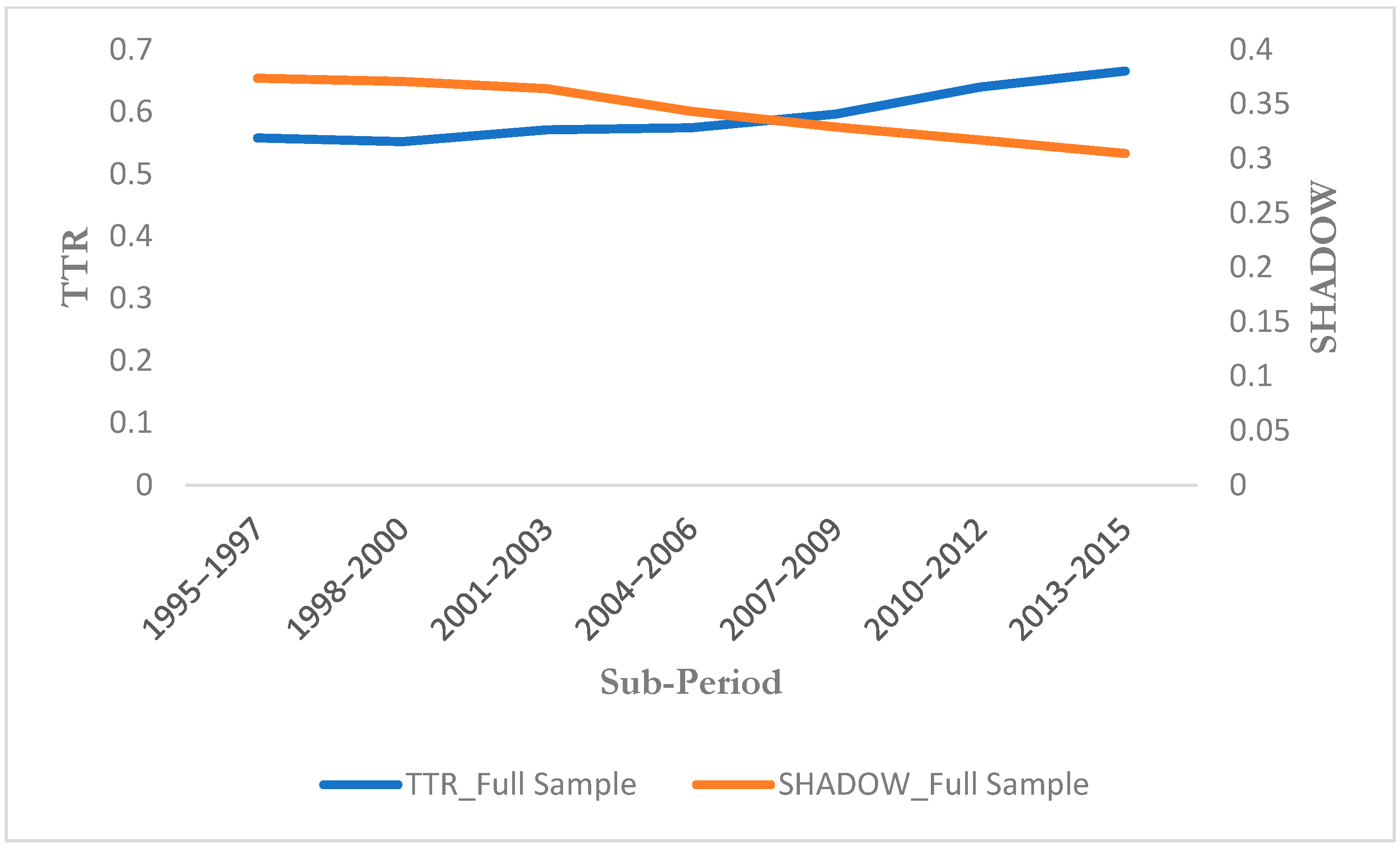
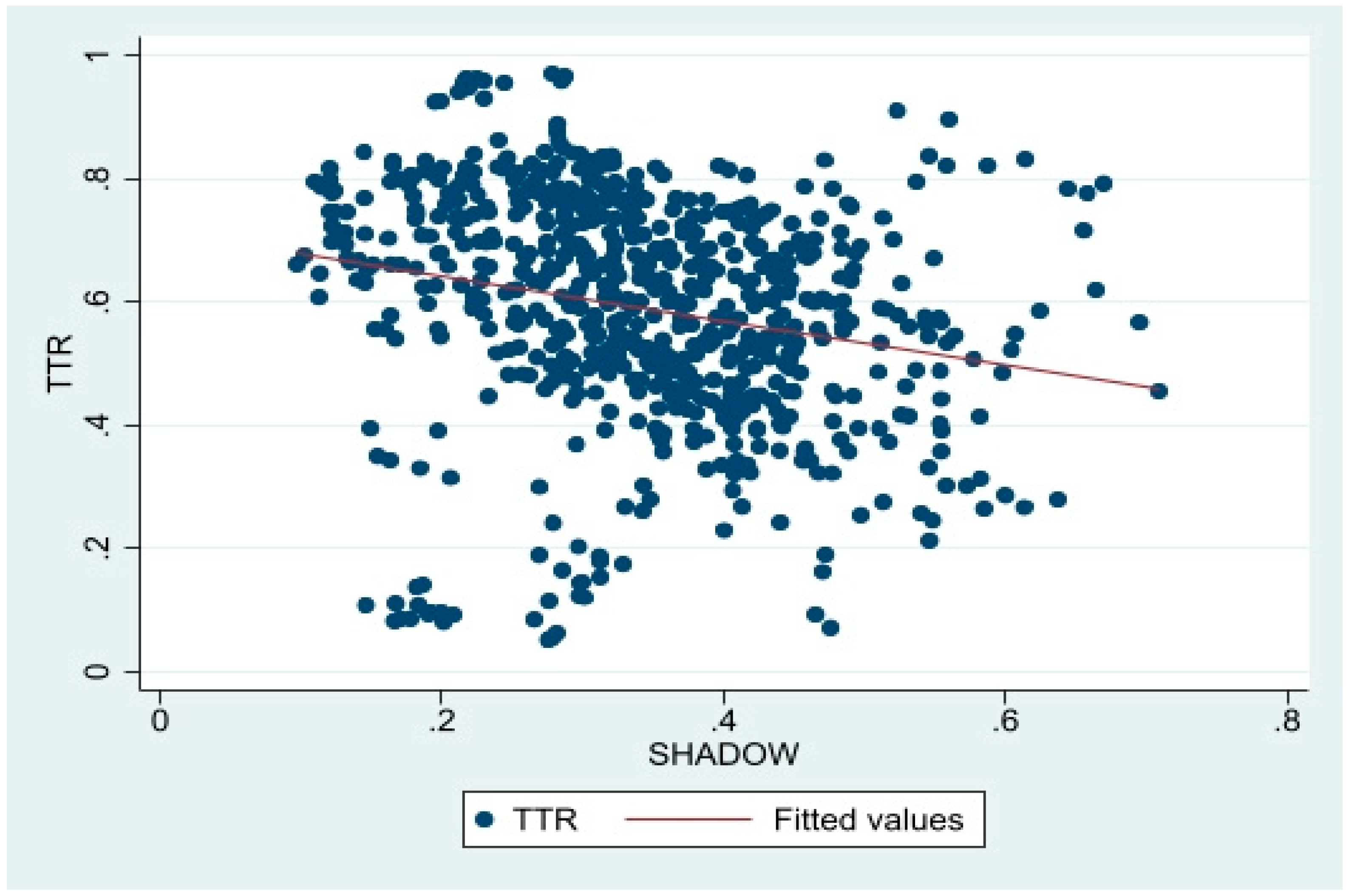
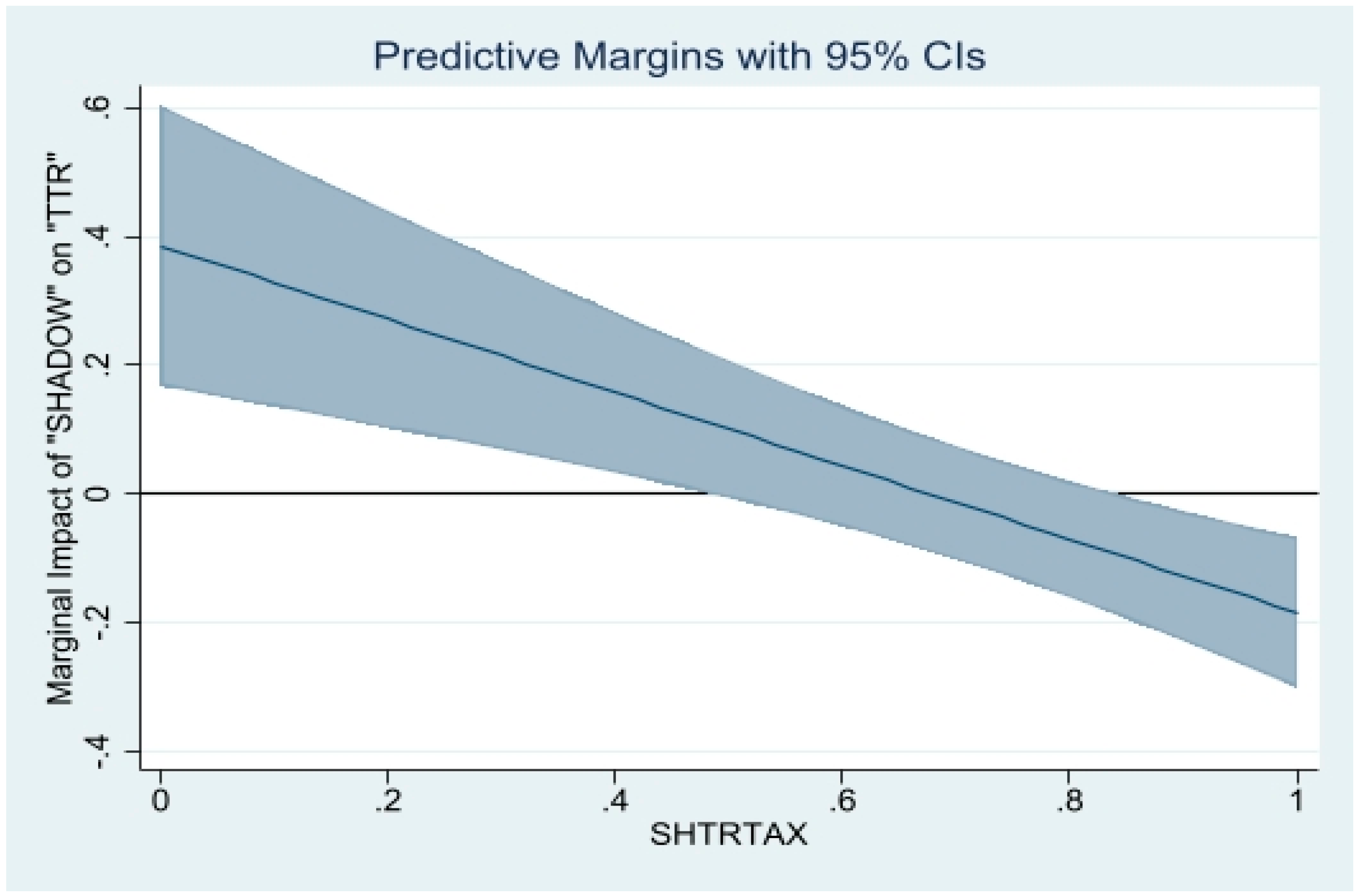
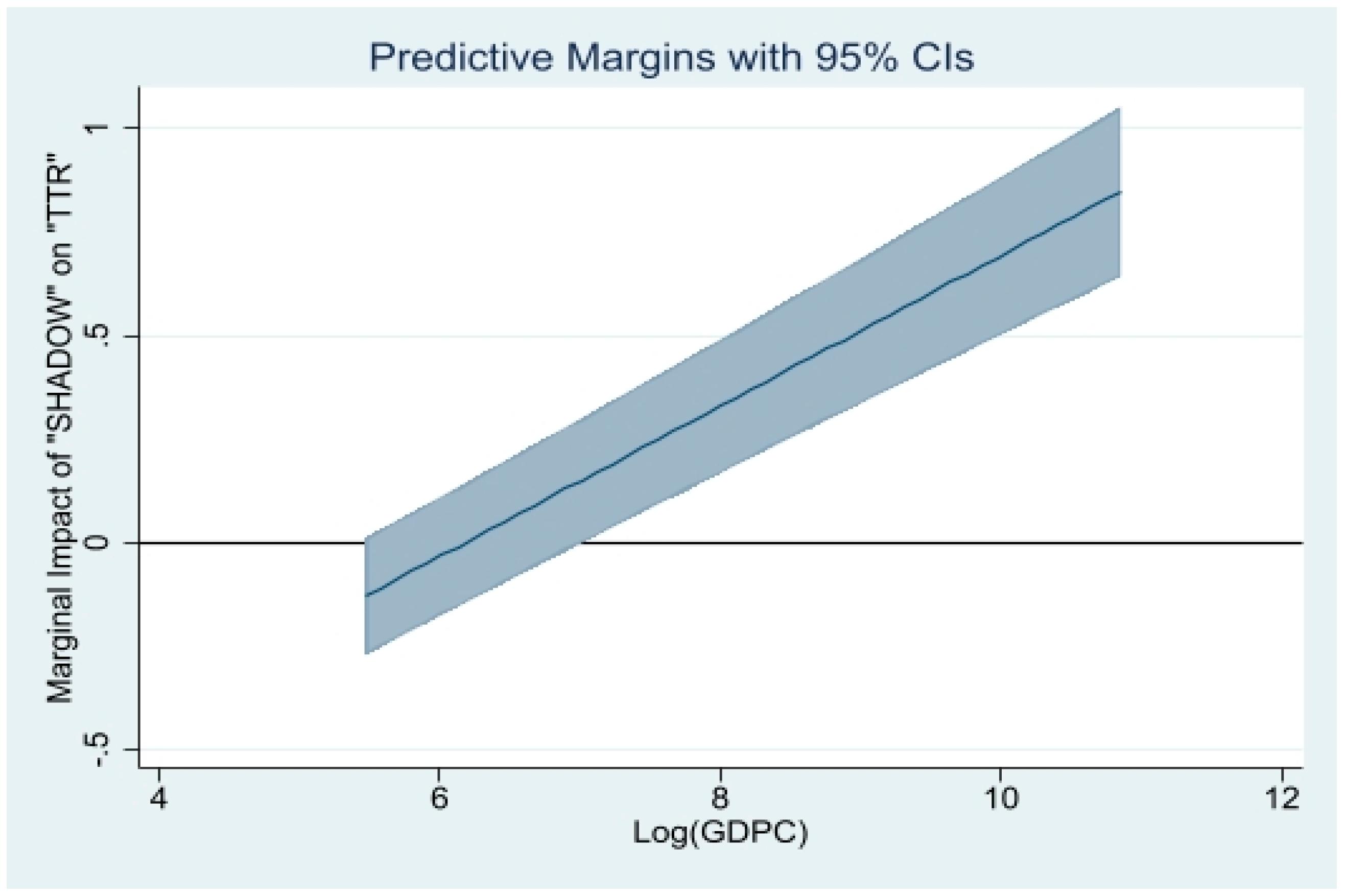
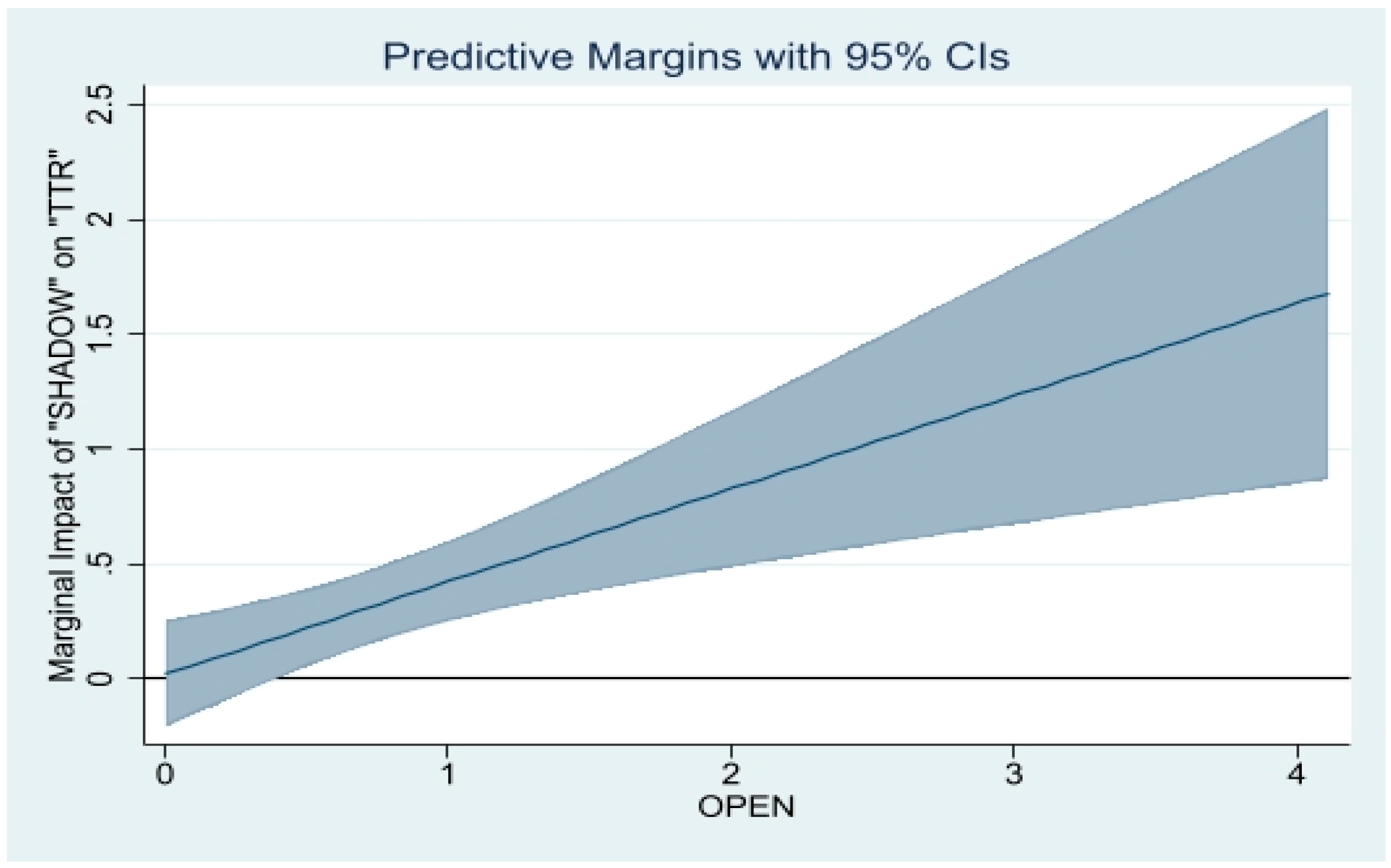
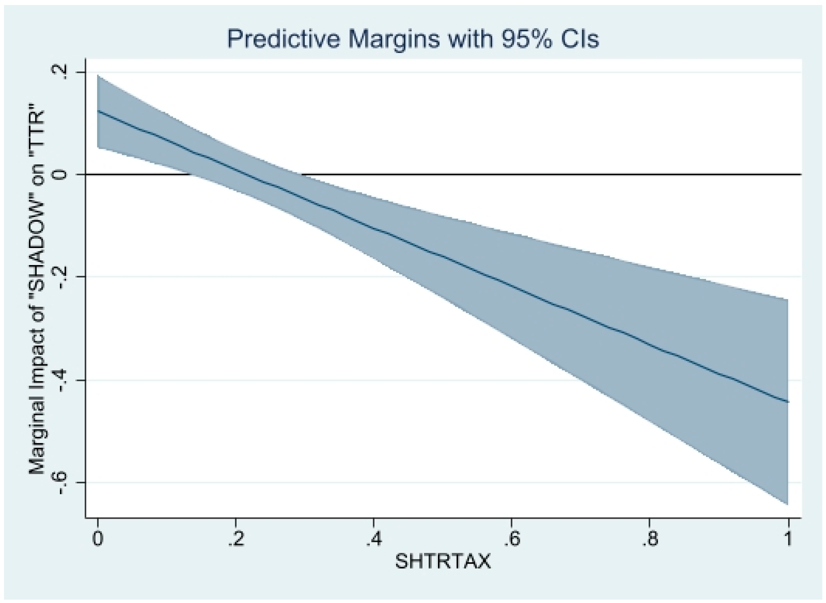
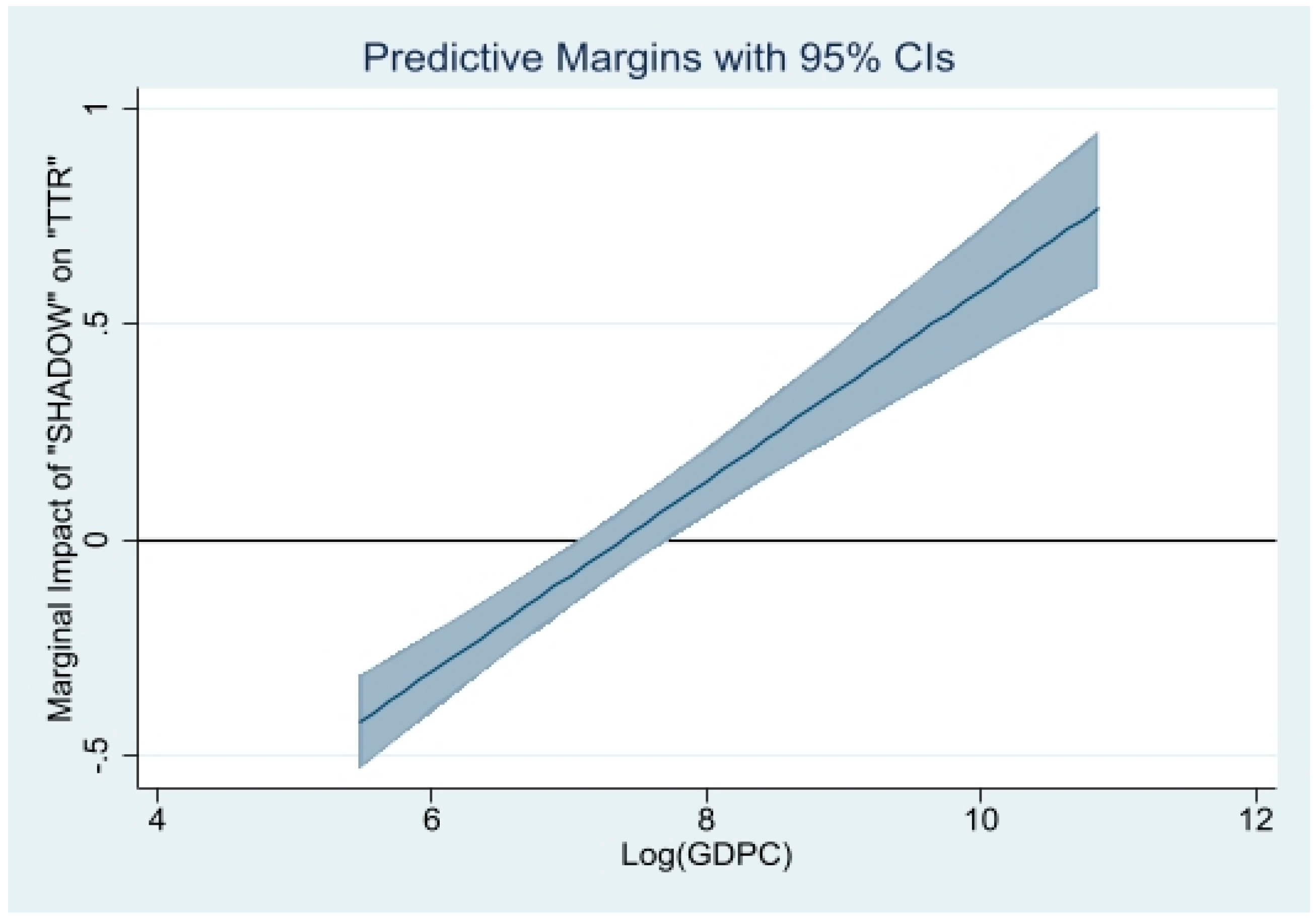
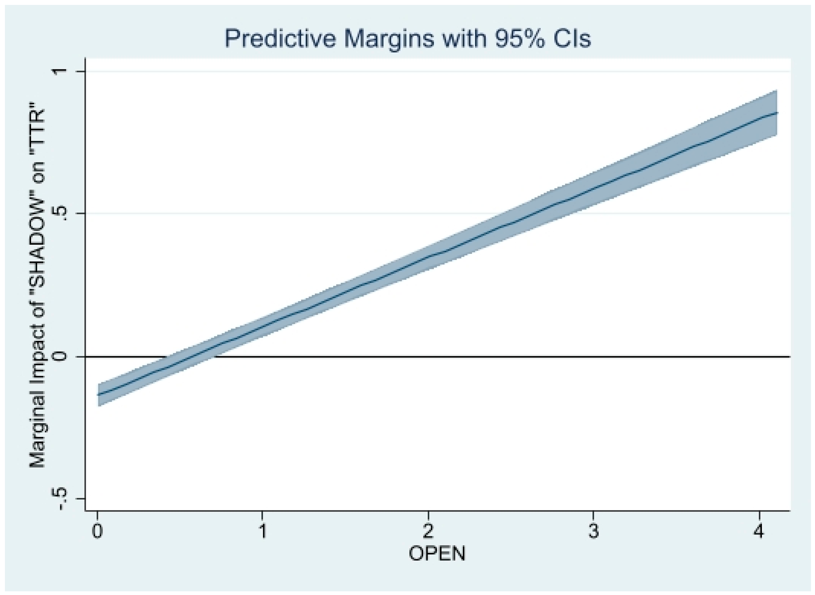
Table A1.
Effect of the shadow economy on revenue-enhancing structural tax reform over the full sample. Estimator: FVW Logit and Probit approaches.
Table A1.
Effect of the shadow economy on revenue-enhancing structural tax reform over the full sample. Estimator: FVW Logit and Probit approaches.
| All Countries | LICs | LICs | ||||
|---|---|---|---|---|---|---|
| Logit | Probit | Logit | Probit | Logit | Probit | |
| Variables | STR | STR | STR | STR | STR | STR |
| (1) | (2) | (3) | (4) | (5) | (6) | |
| SHADOWt−1 | −0.022 ** | −0.019 ** | −0.0399 *** | −0.036 *** | −0.0008 | 0.0008 |
| (0.009) | (0.009) | (0.0139) | (0.0135) | (0.0158) | (0.0154) | |
| Log(GDPC) | −1.149 *** | −0.744 ** | −0.085 | 0.674 | −4.16 *** | −3.248 *** |
| (0.321) | (0.307) | (0.514) | (0.503) | (0.564) | (0.528) | |
| OPENt−1 | −0.0022 | −0.0014 | 0.0018 | 0.0014 | −0.013 *** | −0.015 *** |
| (0.0013) | (0.0011) | (0.0012) | (0.0012) | (0.0035) | (0.003) | |
| RENTt−1 | −0.028 *** | −0.027 *** | −0.028 *** | −0.026 *** | −0.049 *** | −0.037 ** |
| (0.0066) | (0.0066) | (0.008) | (0.0078) | (0.017) | (0.016) | |
| URt−1 | 0.038 *** | 0.035 *** | −0.0036 | −0.013 | −0.020 | −0.028 * |
| (0.011) | (0.010) | (0.0309) | (0.0308) | (0.017) | (0.0152) | |
| GROWTHt−1 | −0.008 | −0.002 | −0.016 ** | −0.009 | 0.006 | 0.003 |
| (0.005) | (0.005) | (0.007) | (0.007) | (0.009) | (0.0096) | |
| INSTt−1 | −0.145 ** | −0.186 *** | −0.2588 *** | −0.374 *** | 0.169 | −0.0112 |
| (0.067) | (0.0652) | (0.085) | (0.084) | (0.110) | (0.1091) | |
| INFLt−1 | 0.0129 | −0.324 | −0.011 | −0.455 | 1.993 ** | 1.921 ** |
| (0.512) | (0.504) | (0.654) | (0.641) | (0.8198) | (0.783) | |
| Log(POP) | 6.300 *** | 5.213 *** | 7.807 *** | 7.733 *** | 4.027 *** | 4.435 *** |
| (0.576) | (0.524) | (1.177) | (1.161) | (1.165) | (1.058) | |
| Observations—Countries | 536-39 | 536-39 | 312-23 | 312-23 | 208-16 | 208-16 |
| Pseudo-R2 | 0.2359 | 0.2189 | 0.3211 | 0.3128 | 0.316 | 0.3060 |
| LR Chi2 (p-value) | 155.34 (0.0000) | 144.17 (0.0000) | 128.42 (0.0000) | 125.07 (0.0000) | 77.11 (0.0001) | 74.74 (0.0002) |
| Log likelihood | −251.594 | −257.18 | −135.739 | −137.415 | 83.589 | −84.774 |
Note: * p-value < 0.1; ** p-value < 0.05; *** p-value < 0.01. Robust Standard Errors are in parentheses. FVW Logit estimator refers to the Fixed Effects Logit estimator proposed by Fernández-Val and Weidner (2016) with the jackknife bias corrections. FVW Probit estimator refers to the Fixed Effects Probit estimator proposed by Fernández-Val and Weidner (2016) with the jackknife bias corrections. Average Partial Effects are reported.
Table A2.
Effect of the shadow economy on revenue-enhancing structural tax reform over the full sample and sub-samples of LICs and EMs. Estimator: 2SLS Probit.
Table A2.
Effect of the shadow economy on revenue-enhancing structural tax reform over the full sample and sub-samples of LICs and EMs. Estimator: 2SLS Probit.
| Full Sample | LICs | EMs | |
|---|---|---|---|
| Dependent Variable | STR | STR | STR |
| (1) | (2) | (3) | |
| SHADOW | −0.097 *** | −0.117 ** | −0.027 |
| (0.035) | (0.047) | (0.038) | |
| Log(GDPC) | −0.283 ** | −0.562 | −0.168 |
| (0.1405) | (0.348) | (0.375) | |
| GROWTHt−1 | −0.004 | −0.037 | −0.015 |
| (0.017) | (0.024) | (0.024) | |
| INFLt−1 | −0.483 | −0.159 | −2.112 |
| (1.200) | (1.723) | (1.850) | |
| OPENt−1 | 0.004 | 0.008 ** | −0.014 ** |
| (0.002) | (0.003) | (0.007) | |
| Log(POP) | −0.064 | −0.062 | −0.033 |
| (0.064) | (0.091) | (0.158) | |
| RENTt−1 | −0.0146 | −0.005 | −0.025 |
| (0.0106) | (0.011) | (0.023) | |
| INSTt−1 | −0.150 | −0.042 | −0.163 |
| (0.106) | (0.123) | (0.176) | |
| URt−1 | 0.028 | 0.034 | 0.0135 |
| (0.021) | (0.039) | (0.022) | |
| Constant | 5.576 ** | 8.0598 * | 3.315 |
| (2.596) | (4.258) | (6.795) | |
| Observations—Countries | 481-40 | 274-24 | 207-16 |
| First Stage Pseudo-R2 | 0.0240 | 0.045 | 0.056 |
| Log likelihood | −289.781 | −167.688 | −113.137 |
| Dependent Variable | SHADOW | SHADOW | SHADOW |
| (1) | (2) | (3) | |
| STR | −47.415 | −8.377 | 14.237 |
| (86.157) | (11.606) | (16.055) | |
| Observations—Countries | 481-40 | 274-24 | 207-16 |
| Adjusted R2 | 0.2403 | 0.3594 | 0.1801 |
Note: * p-value < 0.1; ** p-value < 0.05; *** p-value < 0.01. Robust Standard Errors are in parentheses (corrected standard errors are reported in brackets—see Keshk 2003). To save space, we have not reported results of control variables on the equation of the determinants of the shadow economy. It appeared that many control variables were not significant here, reflecting opposing effects of these control variables across various tax policy and revenue administration areas.
Table A3.
Effect of the shadow economy on different areas of revenue-enhancing structural tax reform over the full sample. Estimator: 2SLS Probit.
Table A3.
Effect of the shadow economy on different areas of revenue-enhancing structural tax reform over the full sample. Estimator: 2SLS Probit.
| Dependent Variable | PIT | CIT | GST | VAT | EXCISE | TRTAX | PROPERTY | SUBSIDIES | REVADM |
|---|---|---|---|---|---|---|---|---|---|
| (1) | (2) | (3) | (4) | (5) | (6) | (7) | (8) | (9) | |
| SHADOW | −0.097 ** | −0.062 * | −0.257 *** | −0.035 | −0.102 *** | −0.092 * | −0.263 *** | −0.1095 | −0.085 ** |
| (0.043) | (0.0355) | (0.069) | (0.035) | (0.0377) | (0.0486) | (0.098) | (0.1009) | (0.034) | |
| Log(GDPC) | −0.9266 *** | −0.053 | −2.090 *** | −0.575 *** | −0.445 *** | −0.176 | −1.439 *** | −1.652 *** | −0.462 *** |
| (0.2068) | (0.144) | (0.377) | (0.151) | (0.1535) | (0.198) | (0.444) | (0.6166) | (0.1416) | |
| GROWTHt−1 | −0.007 | −0.002 | −0.064 * | −0.008 | −0.023 | 0.0256 | −0.034 | 0.0265 | −0.004 |
| (0.022) | (0.018) | (0.033) | (0.017) | (0.019) | (0.023) | (0.047) | (0.0388) | (0.017) | |
| INFLt−1 | −0.340 | −2.430 | −1.08 | −1.022 | 0.878 | 0.775 | −5.252 | −3.27 | −0.257 |
| (1.716) | (1.525) | (2.691) | (1.364) | (1.248) | (1.74) | (4.355) | (4.767) | (1.206) | |
| OPENt−1 | 0.0097 *** | 0.007 *** | 0.017 *** | 0.0025 | 0.001 | −0.008 ** | −0.0088 | −0.043 ** | 0.0054 ** |
| (0.003) | (0.002) | (0.004) | (0.0024) | (0.002) | (0.00366) | (0.0096) | (0.0209) | (0.0023) | |
| Log(POP) | 0.013 | 0.063 | −0.688 *** | 0.046 | −0.108 | −0.317 *** | −0.018 | −0.876 *** | −0.0995 |
| (0.087) | (0.066) | (0.155) | (0.067) | (0.069) | (0.0906) | (0.169) | (0.310) | (0.0634) | |
| RENTt−1 | −0.041 ** | −0.027 ** | −0.051 ** | −0.021 | −0.024 * | −0.054 ** | −0.1103 | −0.015 | −0.012 |
| (0.0155) | (0.0114) | (0.024) | (0.011) | (0.012) | (0.0216) | (0.0536) | (0.043) | (0.010) | |
| INSTt−1 | 0.052 | −0.324 *** | 0.241 | 0.041 | −0.098 | −0.126 | 0.037 | 0.032 | −0.073 |
| (0.145) | (0.1196) | (0.19) | (0.111) | (0.115) | (0.134) | (0.265) | (0.2909) | (0.105) | |
| URt−1 | 0.091 *** | 0.0495 ** | 0.0674 * | 0.066 *** | 0.025 | −0.011 | 0.1315 ** | 0.283 *** | 0.032 |
| (0.027) | (0.0216) | (0.0406) | (0.021) | (0.023) | (0.029) | (0.0566) | (0.0756) | (0.020) | |
| Constant | 7.903 ** | −0.393 | 32.738 *** | 3.482 | 7.784 *** | 8.82 | 18.947 ** | 27.128 *** | 6.9045 *** |
| (3.273) | (2.578) | (6.385) | (2.576) | (2.834) | (3.818) | (7.549) | (9.138) | (2.569) | |
| Observations—Countries | 481-40 | 481-40 | 481-40 | 481-40 | 481-40 | 481-40 | 481-40 | 481-40 | 481-40 |
| First Stage Pseudo-R2 | 0.1059 | 0.055 | 0.3266 | 0.0606 | 0.0338 | 0.1028 | 0.3064 | 0.471 | 0.0338 |
| Log likelihood | −154.713 | −195.108 | −92.769 | −209.270 | −252.224 | −129.961 | −53.265 | −31.591 | −278.549 |
| Dependent Variable | SHADOW | SHADOW | SHADOW | SHADOW | SHADOW | SHADOW | SHADOW | SHADOW | SHADOW |
| (1) | (2) | (3) | (4) | (5) | (6) | (7) | (8) | (9) | |
| Indicator of the type (area) of structural tax reform | 1.753 | −0.179 | 2.798 *** | 3.807 * | 26.826 | 4.142 *** | 0.797 | 1.343 ** | 14.562 |
| (1.484) | (1.447) | (0.946) | (3.416) | (31.182) | (1.4099) | (0.627) | (0.584) | (32.248) | |
| Observations—Countries | 481-40 | 481-40 | 481-40 | 481-40 | 481-40 | 481-40 | 481-40 | 481-40 | 481-40 |
| Adjusted R2 | 0.2011 | 0.1984 | 0.2350 | 0.2021 | 0.2405 | 0.2526 | 0.203 | 0.2267 | 0.2014 |
Note: * p-value < 0.1; ** p-value < 0.05; *** p-value < 0.01. Robust Standard Errors are in parentheses. Corrected standard errors are reported in brackets (see Keshk 2003). To save space, we have not reported results of control variables on the equation of the determinants of the shadow economy. It appeared that the coefficients of many control variables have significant coefficients, in line with the theoretical expectations.
Table A4.
Correlation between the shadow economy and tax transition reform. Estimator: FEDK.
| Variables | TTR | TTR | TTR | TTR | TTR |
|---|---|---|---|---|---|
| (1) | (2) | (3) | (4) | (5) | |
| SHADOW | 0.241 *** | 0.386 *** | 0.415 *** | −1.124 *** | 0.0221 |
| (0.0870) | (0.111) | (0.0976) | (0.0937) | (0.118) | |
| SHADOW*SHTRTAX | −0.570 *** | ||||
| (0.141) | |||||
| SHADOW*LICs | −0.374 *** | ||||
| (0.0442) | |||||
| SHADOW*Log(GDP) | 0.182 *** | ||||
| (0.0126) | |||||
| SHADOW*OPEN | 0.403 *** | ||||
| (0.119) | |||||
| SHTRTAX | −0.0597 *** | 0.111 *** | −0.0595 *** | −0.0517 *** | −0.0504 *** |
| (0.0139) | (0.0373) | (0.0139) | (0.0139) | (0.0140) | |
| Log(GDPC) | 0.0962 *** | 0.103 *** | 0.104 *** | 0.0422 *** | 0.115 *** |
| (0.0130) | (0.0148) | (0.0142) | (0.0133) | (0.0108) | |
| OPEN | 0.0380 *** | 0.0412 *** | 0.0400 *** | 0.0515 *** | −0.0794 *** |
| (0.00668) | (0.00702) | (0.00666) | (0.00894) | (0.0284) | |
| RENT | −0.293 *** | −0.293 *** | −0.276 *** | −0.287 *** | −0.301 *** |
| (0.0562) | (0.0628) | (0.0590) | (0.0540) | (0.0491) | |
| UR | 0.241 *** | 0.225 *** | 0.155 *** | 0.0616 * | 0.140 *** |
| (0.0473) | (0.0471) | (0.0488) | (0.0333) | (0.0374) | |
| GROWTH | 0.160 *** | 0.147 *** | 0.144 *** | 0.120 *** | 0.124 *** |
| (0.0262) | (0.0167) | (0.0257) | (0.0279) | (0.0288) | |
| INST | 0.0229 *** | 0.0227 *** | 0.0211 *** | 0.0201 *** | 0.0213 *** |
| (0.00443) | (0.00465) | (0.00431) | (0.00376) | (0.00426) | |
| INFL | −0.0372 * | −0.0374 ** | −0.0445 ** | −0.0417 ** | −0.0388 * |
| (0.0207) | (0.0184) | (0.0203) | (0.0192) | (0.0202) | |
| Log(POP) | 0.207 *** | 0.192 *** | 0.186 *** | 0.186 *** | 0.199 *** |
| (0.0211) | (0.0200) | (0.0175) | (0.0174) | (0.0195) | |
| Constant | −3.576 *** | −3.441 *** | −3.305 *** | −2.828 *** | −3.525 *** |
| (0.426) | (0.412) | (0.375) | (0.369) | (0.407) | |
| Observations—Countries | 666-114 | 666-114 | 666-114 | 666-114 | 666-114 |
| Within R-squared | 0.3741 | 0.3841 | 0.3841 | 0.3975 | 0.4008 |
Note: * p-value < 0.1; ** p-value < 0.05; *** p-value < 0.01. Robust Standard Errors are in parentheses.
Table A5.
Effect of the shadow economy on tax transition reform. Estimator: Method of Moments Quantile Regression (MMQR).
Table A5.
Effect of the shadow economy on tax transition reform. Estimator: Method of Moments Quantile Regression (MMQR).
| Variables | Location a | Scale b | Q10th | Q20th | Q30th | Q40th | Q50th | Q60th | Q70th | Q80th | Q90th |
|---|---|---|---|---|---|---|---|---|---|---|---|
| (1) | (2) | (3) | (4) | (5) | (6) | (7) | (8) | (9) | (10) | (11) | |
| SHADOW | 0.265 *** | −0.0610 | 0.356 *** | 0.333 *** | 0.313 *** | 0.289 *** | 0.262 *** | 0.236 ** | 0.215 ** | 0.195 * | 0.163 |
| (0.0953) | (0.0451) | (0.116) | (0.106) | (0.101) | (0.0967) | (0.0955) | (0.0983) | (0.103) | (0.110) | (0.123) | |
| SHTRTAX | −0.0668 ** | 0.0286 ** | −0.110 *** | −0.0989 *** | −0.0891 *** | −0.0783 *** | −0.0656 ** | −0.0533 * | −0.0436 | −0.0341 | −0.0188 |
| (0.0275) | (0.0143) | (0.0347) | (0.0316) | (0.0295) | (0.0281) | (0.0276) | (0.0284) | (0.0299) | (0.0320) | (0.0365) | |
| Log(GDPC) | 0.152 *** | −0.00427 | 0.158 *** | 0.157 *** | 0.155 *** | 0.154 *** | 0.152 *** | 0.150 *** | 0.148 *** | 0.147 *** | 0.145 *** |
| (0.0329) | (0.0185) | (0.0524) | (0.0466) | (0.0418) | (0.0371) | (0.0325) | (0.0297) | (0.0288) | (0.0292) | (0.0325) | |
| OPEN | 0.0517 *** | 0.00945 | 0.0375 ** | 0.0411 *** | 0.0443 *** | 0.0479 *** | 0.0521 *** | 0.0561 *** | 0.0593 *** | 0.0625 *** | 0.0675 *** |
| (0.0127) | (0.00615) | (0.0155) | (0.0143) | (0.0135) | (0.0129) | (0.0128) | (0.0131) | (0.0138) | (0.0147) | (0.0166) | |
| RENT | −0.308 *** | −0.0196 | −0.279 *** | −0.286 *** | −0.293 *** | −0.301 *** | −0.309 *** | −0.318 *** | −0.324 *** | −0.331 *** | −0.341 ** |
| (0.0958) | (0.0480) | (0.103) | (0.0965) | (0.0931) | (0.0925) | (0.0965) | (0.104) | (0.113) | (0.123) | (0.141) | |
| UR | 0.203 * | 0.0472 | 0.133 | 0.150 | 0.167 | 0.184 | 0.205 * | 0.226 ** | 0.242 ** | 0.257 ** | 0.282 ** |
| (0.109) | (0.0491) | (0.139) | (0.128) | (0.120) | (0.113) | (0.108) | (0.108) | (0.110) | (0.115) | (0.127) | |
| GROWTH | 0.132 | −0.0140 | 0.153 | 0.148 | 0.143 | 0.138 | 0.132 | 0.126 | 0.121 | 0.116 | 0.109 |
| (0.0843) | (0.0461) | (0.123) | (0.110) | (0.100) | (0.0912) | (0.0838) | (0.0812) | (0.0824) | (0.0862) | (0.0974) | |
| INST | 0.0137 ** | −0.00375 | 0.0193 ** | 0.0179 ** | 0.0166 ** | 0.0152 ** | 0.0136 * | 0.0119 * | 0.0107 | 0.00943 | 0.00742 |
| (0.00699) | (0.00323) | (0.00927) | (0.00852) | (0.00791) | (0.00738) | (0.00698) | (0.00686) | (0.00695) | (0.00723) | (0.00799) | |
| INFL | −0.0709 ** | 0.0289 ** | −0.114 *** | −0.103 *** | −0.0935 *** | −0.0826 ** | −0.0697 ** | −0.0573 | −0.0475 | −0.0380 | −0.0225 |
| (0.0340) | (0.0128) | (0.0358) | (0.0342) | (0.0335) | (0.0336) | (0.0343) | (0.0358) | (0.0375) | (0.0397) | (0.0433) | |
| Log(POP) | 0.298 *** | 0.0153 | 0.275 *** | 0.281 *** | 0.286 *** | 0.292 *** | 0.299 *** | 0.305 *** | 0.310 *** | 0.315 *** | 0.324 *** |
| (0.0416) | (0.0207) | (0.0573) | (0.0522) | (0.0480) | (0.0443) | (0.0415) | (0.0405) | (0.0412) | (0.0430) | (0.0478) | |
| Constant | −5.486 *** | −0.177 | −5.221 *** | −5.287 *** | −5.348 *** | −5.414 *** | −5.493 *** | −5.569 *** | −5.629 *** | −5.687 *** | −5.781 *** |
| (0.883) | (0.461) | (1.280) | (1.156) | (1.054) | (0.959) | (0.878) | (0.841) | (0.844) | (0.875) | (0.974) | |
| Observations—Countries | 666-114 | 666-114 | 666-114 | 666-114 | 666-114 | 666-114 | 666-114 | 666-114 | 666-114 | 666-114 | 666-114 |
Note: * p-value < 0.1; ** p-value < 0.05; *** p-value < 0.01. Robust Standard Errors are in parentheses. (a) indicates the location parameters, and (b) refers to the scale parameters.
Table A6.
Effect of the shadow economy on the tax transition reform Estimator: Method of Moments Quantile Regression (MMQR).
Table A6.
Effect of the shadow economy on the tax transition reform Estimator: Method of Moments Quantile Regression (MMQR).
| Effect of the Shadow Economy on Tax Transition Reform Conditioned on the Share of Trade Tax Revenue in Non-Resource Tax Revenue | |||||||||||
|---|---|---|---|---|---|---|---|---|---|---|---|
| Variables | Location a | Scale b | Q10th | Q20th | Q30th | Q40th | Q50th | Q60th | Q70th | Q80th | Q90th |
| (1) | (2) | (3) | (4) | (5) | (6) | (7) | (8) | (9) | (10) | (11) | |
| SHADOW*SHTRTAX | −0.535 *** | 0.0500 | −0.609 ** | −0.591 ** | −0.574 *** | −0.555 *** | −0.532 *** | −0.510 *** | −0.494 *** | −0.477 *** | −0.450 ** |
| (0.177) | (0.102) | (0.269) | (0.242) | (0.217) | (0.194) | (0.175) | (0.166) | (0.167) | (0.175) | (0.199) | |
| SHADOW | 0.405 *** | −0.0988 * | 0.552 *** | 0.517 *** | 0.482 *** | 0.444 *** | 0.400 *** | 0.356 *** | 0.325 *** | 0.291 ** | 0.238 * |
| (0.115) | (0.0592) | (0.161) | (0.146) | (0.134) | (0.123) | (0.114) | (0.111) | (0.113) | (0.118) | (0.131) | |
| SHTRTAX | 0.0931 ** | −0.00291 | 0.0974 | 0.0964 | 0.0954 * | 0.0943 * | 0.0929 ** | 0.0917 ** | 0.0908 ** | 0.0897 ** | 0.0882 * |
| (0.0457) | (0.0262) | (0.0710) | (0.0639) | (0.0571) | (0.0508) | (0.0451) | (0.0420) | (0.0417) | (0.0432) | (0.0488) | |
| Turning point of “SHTRTAX” | 0.906 (=0.552/0.609) | 0.875 (=0.517/0.591) | 0.85 (=0.482/0.574) | 0.8 (=0.444/0.555) | 0.752 (=0.400/0.532) | 0.698 (=0.356/0.510) | 0.658 (=0.325/0.494) | 0.61 (=0.291/0.477) | 0.529 (=0.238/0.450) | ||
| Effect of the Shadow Economy on Tax Transition Reform Conditioned on the Real per Capita Income | |||||||||||
| Variables | Location a | Scale b | Q10th | Q20th | Q30th | Q40th | Q50th | Q60th | Q70th | Q80th | Q90th |
| (1) | (2) | (3) | (4) | (5) | (6) | (7) | (8) | (9) | (10) | (11) | |
| SHADOW*Log(GDP) | 0.146 *** | −0.00657 | 0.156 *** | 0.153 *** | 0.151 *** | 0.149 *** | 0.146 *** | 0.143 *** | 0.140 *** | 0.138 *** | 0.135 ** |
| (0.0472) | (0.0192) | (0.0573) | (0.0535) | (0.0506) | (0.0485) | (0.0472) | (0.0475) | (0.0487) | (0.0507) | (0.0549) | |
| SHADOW | −0.829 ** | −0.0513 | −0.752 * | −0.771 * | −0.790 ** | −0.808 ** | −0.832 ** | −0.854 ** | −0.872 ** | −0.889 ** | −0.914 ** |
| (0.359) | (0.150) | (0.427) | (0.400) | (0.379) | (0.365) | (0.359) | (0.365) | (0.379) | (0.397) | (0.434) | |
| Log(GDPC) | 0.0908 *** | −0.00843 | 0.104 ** | 0.100 ** | 0.0973 ** | 0.0943 ** | 0.0904 *** | 0.0867 *** | 0.0837 ** | 0.0810 ** | 0.0768 ** |
| (0.0349) | (0.0183) | (0.0513) | (0.0462) | (0.0418) | (0.0381) | (0.0346) | (0.0331) | (0.0331) | (0.0342) | (0.0377) | |
| Effect of the Shadow Economy on Tax Transition Reform Conditioned on the Level of Trade Openness | |||||||||||
| Variables | Location a | Scale b | Q10th | Q20th | Q30th | Q40th | Q50th | Q60th | Q70th | Q80th | Q90th |
| (1) | (2) | (3) | (4) | (5) | (6) | (7) | (8) | (9) | (10) | (11) | |
| SHADOW*OPEN | 0.388 *** | 0.0574 | 0.298 * | 0.325 ** | 0.343 ** | 0.363 *** | 0.386 *** | 0.416 *** | 0.434 *** | 0.452 *** | 0.485 *** |
| (0.110) | (0.0525) | (0.173) | (0.152) | (0.138) | (0.125) | (0.111) | (0.0959) | (0.0897) | (0.0868) | (0.0890) | |
| SHADOW | 0.0589 | −0.109 * | 0.229 | 0.179 | 0.144 | 0.107 | 0.0624 | 0.00607 | −0.0290 | −0.0621 | −0.125 |
| (0.121) | (0.0584) | (0.173) | (0.153) | (0.142) | (0.132) | (0.122) | (0.117) | (0.116) | (0.120) | (0.131) | |
| OPEN | −0.0635 | −0.00962 | −0.0484 | −0.0529 | −0.0559 | −0.0592 | −0.0632 | −0.0681 ** | −0.0712 ** | −0.0741 ** | −0.0797 ** |
| (0.0396) | (0.0187) | (0.0622) | (0.0549) | (0.0500) | (0.0452) | (0.0400) | (0.0347) | (0.0325) | (0.0313) | (0.0319) | |
Note: * p-value < 0.1; ** p-value < 0.05; *** p-value < 0.01. Robust Standard Errors are in parentheses. (a) indicates the location parameters, and (b) refers to the scale parameters. For the sake of brevity, we report here the outcomes concerning variables of key interest in the analysis. Estimates concerning other control variables are similar to those presented in Table A5 and can be obtained upon request.
Table A7.
Effect of the shadow economy on tax transition reform Estimator: Two-Step System GMM.
| Variables | TTR | TTR | TTR | TTR | TTR |
|---|---|---|---|---|---|
| (1) | (2) | (3) | (4) | (5) | |
| TTRt−1 | 0.495 *** | 0.520 *** | 0.522 *** | 0.458 *** | 0.499 *** |
| (0.0143) | (0.0137) | (0.0119) | (0.0188) | (0.0116) | |
| SHADOW | 0.0723 ** | 0.123 *** | 0.192 *** | −1.632 *** | −0.139 *** |
| (0.0301) | (0.0357) | (0.0342) | (0.176) | (0.0203) | |
| SHADOW*SHTRTAX | −0.567 *** | ||||
| (0.129) | |||||
| SHADOW*LICs | −0.202 *** | ||||
| (0.0394) | |||||
| SHADOW*Log(GDP) | 0.221 *** | ||||
| (0.0237) | |||||
| SHADOW*OPEN | 0.242 *** | ||||
| (0.0114) | |||||
| LICs | 0.0762 *** | ||||
| (0.0214) | |||||
| SHTRTAX | −0.159 *** | −0.0165 | −0.133 *** | −0.163 *** | −0.160 *** |
| (0.0180) | (0.0512) | (0.0141) | (0.0222) | (0.0164) | |
| Log(GDPC) | −0.0171 *** | −0.0170 *** | −0.00111 | −0.0883 *** | −0.0165 *** |
| (0.00410) | (0.00232) | (0.00465) | (0.00811) | (0.00238) | |
| OPEN | 0.0187 *** | 0.0189 *** | 0.0151 *** | 0.0368 *** | −0.0467 *** |
| (0.00552) | (0.00452) | (0.00480) | (0.00528) | (0.00306) | |
| RENT | −0.297 *** | −0.279 *** | −0.293 *** | −0.288 *** | −0.288 *** |
| (0.0224) | (0.0174) | (0.0161) | (0.0214) | (0.0129) | |
| UR | 0.0586 | 0.0238 | −0.00910 | 0.0559 | −0.00349 |
| (0.0485) | (0.0392) | (0.0444) | (0.0506) | (0.0437) | |
| GROWTH | 0.515 *** | 0.514 *** | 0.504 *** | 0.425 *** | 0.454 *** |
| (0.0393) | (0.0280) | (0.0375) | (0.0377) | (0.0275) | |
| INST | 0.0191 *** | 0.0179 *** | 0.0188 *** | 0.0256 *** | 0.0239 *** |
| (0.00314) | (0.00233) | (0.00162) | (0.00341) | (0.00186) | |
| INFL | 0.0191 | 0.0312 *** | 0.00267 | 0.0469 *** | 0.00553 |
| (0.0158) | (0.0112) | (0.0107) | (0.0147) | (0.0103) | |
| Log(POP) | 0.00578 ** | 0.00511 *** | 0.00436 * | 0.00690 ** | 0.00517 ** |
| (0.00278) | (0.00166) | (0.00234) | (0.00288) | (0.00212) | |
| Observations—Countries | 555-114 | 555-114 | 555-114 | 555-114 | 555-114 |
| AR1 (p-value) | 0.0270 | 0.0269 | 0.0263 | 0.0327 | 0.0283 |
| AR2 (p-value) | 0.1207 | 0.1094 | 0.10 | 0.10 | 0.1087 |
| OID (p-value) | 0.3849 | 0.5027 | 0.4040 | 0.4127 | 0.3012 |
Note: * p-value < 0.1; ** p-value < 0.05; *** p-value < 0.01. Robust Standard Errors are in parentheses. The variables “SHADOW”, “SHTRTAX”, “OPEN”, “GROWTH”, “UR”, “INFL”, “INST”, “RENT”, and the interaction variables have been treated as endogenous. The variable “POP” has been considered as exogenous. Time dummies have been included in the regressions. The latter have used 2 lags of endogenous variables as instruments.
Appendix A.1. Definition and Source of Variables
| Variables | Definition | Source |
| STR | This is the first indicator of revenue-enhancing structural tax reform. It identifies the episodes of large tax revenue mobilization identified over the period from 2000 to 2015 (see Akitoby et al. 2020). The variable “STR” takes the value of 1 for a year characterized by a large revenue mobilization and the value of 0 for other years. The different areas of tax policy and revenue administration where major reforms took place are as follows: Personal Income Tax (“PIT”); Corporate Income Tax (“CIT”); Goods and Services Tax (“GST”); Value Added Tax (“VAT”); Excise Tax (“EXCISE”); Trade Tax (“TRTAX”); Property Tax (“PROPERTY”); Subsidies (“SUBSIDIES”); and Revenue Administration (“REVADM”). | Data extracted from Akitoby et al. (2020) |
| TTR | This is the second indicator of tax reform, referred to as ‘tax transition reform’. It reflects the extent of the reform of the tax revenue structure towards a lower dependence of the non-resource tax revenue on international trade tax revenue (and hence in favor of a greater dependence of the non-resource tax revenue on domestic tax revenue). Practically, it captures the convergence of the tax revenue structure of a given developing country towards the developed countries’ tax revenue structure. Its values range between 0 and 100, with higher values reflecting greater tax revenue structure convergence, i.e., greater tax reforms. | Author’s computation (see Section 3.2.1) based on data extracted from the ‘UNU-WIDER Government Revenue Dataset’. Version 2021. https://www.wider.unu.edu/project/grd-%E2%80%93-government-revenue-dataset (Accessed in 20 June 2021). |
| SHADOW | This is the measure of the share of the size of the shadow economy in the official GDP. It has been computed by Medina and Schneider (2018) using the multiple indicators, multiple causes (MIMIC) method. The latter extracts covariance information from observable variables classified as causes or indicators of the latent shadow economy (see Schneider et al. 2010 for more details on this approach). | Data extracted from Medina and Schneider (2018) |
| SHTRTAX | This is the share of international trade tax revenue in total non-resource tax revenue. Non-resource tax revenue is the difference between total tax revenue (as a share of GDP, excluding social contributions) and tax revenue collected on natural resources (the latter includes a significant component of economic rent, primarily from oil and mining activities) as a share of GDP. | Author’s calculation based on data extracted from the UNU-WIDER Government Revenue Dataset’. Version 2021. https://www.wider.unu.edu/project/grd-%E2%80%93-government-revenue-dataset (Accessed in 20 June 2021). |
| GDPC | Real per capita Gross Domestic Product (constant 2015 USD). | World Development Indicators (WDIs) of the World Bank |
| GROWTH | Real Growth Rate of the Gross Domestic Product, annual change (constant 2015 USD). | WDI |
| OPEN | This is the indicator of trade openness, measured by the share (in percentage) of the sum of exports and imports of GDP. | WDI |
| INFL | The variable “INFL” has been calculated using the following formula: INFL (2), where refers to the absolute value of the annual inflation rate (not in percentage), denoted “INFLATION”. The inflation rate is based on Consumer Price Index (CPI), where missing values have been replaced with values of the GDP Deflator. | Authors’ calculation based on data from the WDI. |
| EDU | This is the average of the gross primary school enrollment (in percentage), gross secondary school enrollment (in percentage), and gross tertiary school enrollment (in percentage). | Author’s calculation based on data collected from the WDI. |
| RENT | This is the share of total natural resource rents in GDP. | WDI |
| UR | Rate of total unemployment (i.e., for both male and female) as a share of total labor force. | WDI |
| POP | Total Population | WDI |
| INST | This is the variable capturing the institutional quality. It has been computed by extracting the first principal component (based on factor analysis) of the following six indicators of governance: political stability and absence of violence/terrorism; regulatory quality; rule of law; government effectiveness; voice and accountability; and corruption. Higher values of the index “INST” are associated with better governance and institutional quality, while lower values reflect worse governance and institutional quality. | Data on the components of “INST” variables have been extracted from World Bank Governance Indicators developed by Kaufmann et al. (2010) and updated recently. See online at: https://info.worldbank.org/governance/wgi/ (Accessed in 20 June 2022). |
Appendix A.2. Descriptive Statistics on Variables Used in the Analysis over the Full Sample
| Variable | Observations | Mean | Standard Deviation | Minimum | Maximum |
| STR | 481 | 0.308 | 0.462 | 0 | 1 |
| PIT | 481 | 0.116 | 0.321 | 0 | 1 |
| CIT | 481 | 0.154 | 0.361 | 0 | 1 |
| GST | 481 | 0.083 | 0.276 | 0 | 1 |
| VAT | 481 | 0.175 | 0.380 | 0 | 1 |
| EXCISE | 481 | 0.233 | 0.423 | 0 | 1 |
| TRTAX | 481 | 0.089 | 0.286 | 0 | 1 |
| PROPERTY | 481 | 0.037 | 0.190 | 0 | 1 |
| SUBSIDIES | 481 | 0.027 | 0.162 | 0 | 1 |
| REVADM | 481 | 0.287 | 0.453 | 0 | 1 |
| SHADOW | 481 | 36.104 | 7.869 | 20.380 | 68.460 |
| GROWTH | 481 | 4.320 | 4.360 | −36.392 | 20.716 |
| UR | 481 | 7.782 | 5.388 | 0.390 | 28.640 |
| GDPC | 481 | 3453.151 | 5453.988 | 295.737 | 35,852.240 |
| INFLATION | 481 | 0.064 | 0.067 | −0.043 | 0.738 |
| EDU | 460 | 55.715 | 20.661 | 1.612 | 94.347 |
| OPEN | 480 | 77.687 | 33.455 | 20.964 | 311.354 |
| INST | 444 | −1.100 | 1.336 | −3.750 | 2.989 |
| POP | 481 | 14,100,000 | 20,400,000 | 255,068 | 102,000,000 |
| RENT | 481 | 7.674 | 10.221 | 0.006 | 58.650 |
Appendix A.2.1. Pairwise Correlation Statistics on Variables Used in the Analysis over the Full Sample of 40 LICs and Ems
| STR | PIT | PIT | GST | VAT | EXCISE | TRTAX | PROPERTY | SUBSIDIES | REVADM | |
| STR | 1.0000 | |||||||||
| PIT | 0.5445 * | 1.0000 | ||||||||
| CIT | 0.6396 * | 0.5638 * | 1.0000 | |||||||
| GST | 0.4518 * | 0.3837 * | 0.4142 * | 1.0000 | ||||||
| VAT | 0.6900 * | 0.6184 * | 0.5324 * | 0.4168 * | 1.0000 | |||||
| EXCISE | 0.8264 * | 0.4902 * | 0.5149 * | 0.4576 * | 0.5758 * | 1.0000 | ||||
| TRTAX | 0.4700 * | 0.2043 * | 0.1087 * | 0.3806 * | 0.3549 * | 0.4825 * | 1.0000 | |||
| PROPERTY | 0.2958 * | 0.2017 * | 0.1284 * | 0.1390 * | 0.4286 * | 0.3579 * | 0.1302 * | 1.0000 | ||
| SUBSIDIES | 0.2500 * | 0.1394 * | 0.1777 * | 0.2748 * | 0.2948 * | 0.2115 * | 0.1725 * | −0.0329 | 1.0000 | |
| REVADM | 0.9514 * | 0.5723 * | 0.6085 * | 0.4748 * | 0.7252 * | 0.8142 * | 0.4134 * | 0.3109 * | 0.2628 * | 1.0000 |
| SHADOW | −0.0323 | 0.1021 * | 0.0009 | −0.0080 | 0.0500 | 0.0398 | 0.0204 | −0.0106 | 0.0346 | 0.0066 |
| GROWTH | 0.0869 * | 0.0309 | 0.0170 | −0.0007 | 0.0290 | 0.0398 | 0.0675 | 0.0090 | −0.0555 | 0.0774 * |
| UR | −0.0669 | 0.0565 | 0.0455 | −0.0326 | 0.0520 | −0.0969 * | −0.0476 | −0.0193 | 0.0788 * | −0.0583 |
| GDPC | −0.0840 * | −0.0947 * | −0.0600 | −0.0817 * | −0.0995 * | −0.0787 * | 0.0079 | −0.0216 | −0.0613 | −0.1197 * |
| INFLATION | −0.0411 | −0.0184 | −0.0400 | −0.0676 | −0.0488 | −0.0098 | −0.0071 | −0.0932 * | −0.0345 | −0.0374 |
| EDU | −0.0466 | −0.0478 | −0.0026 | −0.1790 * | 0.0160 | −0.0884 * | −0.0005 | −0.0392 | −0.1330 * | −0.0797 * |
| OPEN | 0.0559 | 0.0641 | 0.1113 * | 0.1057 * | −0.0214 | −0.0363 | −0.0862 * | −0.1194 * | −0.1223 * | 0.0875 * |
| INST | −0.0525 | 0.0317 | −0.0471 | 0.0569 | −0.0012 | −0.0382 | 0.0766 | 0.0373 | −0.0452 | −0.0617 |
| POP | 0.0421 | −0.0763 * | 0.0761 * | −0.1362 * | −0.0483 | 0.0490 | −0.0081 | 0.0120 | −0.0964 * | −0.0259 |
| RENT | 0.0554 | −0.0661 | 0.0049 | 0.0076 | −0.0629 | −0.0085 | −0.0871 * | −0.0570 | −0.0399 | 0.0597 |
| Note: * p-value < 0.1. | ||||||||||
Appendix A.2.2. (Continued): Pairwise Correlation Statistics on Variables Used in the Analysis over the Full Sample of 40 LICs and EMs
| SHADOW | GROWTH | UR | GDPC | INFLATION | EDU | OPEN | INST | POP | RENT | |
| SHADOW | 1.0000 | |||||||||
| GROWTH | −0.0616 | 1.0000 | ||||||||
| UR | 0.0592 | −0.1413 * | 1.0000 | |||||||
| GDPC | −0.1950 * | −0.1570 * | 0.2600 * | 1.0000 | ||||||
| INFLATION | 0.0659 | −0.1049 * | −0.1367 * | −0.0867 * | 1.0000 | |||||
| EDU | −0.0296 | 0.0223 | 0.1369 * | 0.2237 * | 0.0071 | 1.0000 | ||||
| OPEN | 0.0278 | 0.0480 | 0.2635 * | 0.0584 | −0.0350 | 0.2392 * | 1.0000 | |||
| INST | −0.1968 * | −0.0366 | 0.4596 * | 0.6609 * | −0.1875 * | 0.3124 * | 0.1120 * | 1.0000 | ||
| POP | −0.1467 * | 0.0610 | −0.1418 * | −0.0357 | 0.0747 | 0.1044 * | −0.1956 * | −0.0459 | 1.0000 | |
| RENT | −0.0512 | 0.0078 | −0.0397 | −0.2065 * | 0.0372 | −0.2887 * | 0.0837 * | −0.5100 * | −0.0748 | 1.0000 |
| Note: * p-value < 0.1. The variables “SHADOW”, “OPEN”, “UR”, “GROWTH”, and “RENT” are expressed in percentage. | ||||||||||
Appendix A.3. List of the 40 Developing Countries Contained in the Full Sample, including Low-Income Countries (LICs) and Emerging Markets (EMs)
| Full Sample (40 Developing Countries) | LICs | EMs | |
| Algeria | Mauritania | Burkina Faso | Algeria |
| Armenia | Moldova | Burundi | Armenia |
| Bahamas, The | Morocco | Cabo Verde | Bahamas, The |
| Belize | Namibia | Cambodia | Belize |
| Bosnia and Herzegovina | Nepal | Central African Republic | Bosnia and Herzegovina |
| Bulgaria | Nicaragua | Comoros | Bulgaria |
| Burkina Faso | Paraguay | Congo, Rep. | Ecuador |
| Burundi | Philippines | Gambia, The | Georgia |
| Cabo Verde | Rwanda | Guinea | Jamaica |
| Cambodia | Senegal | Guinea-Bissau | Morocco |
| Central African Republic | Sierra Leone | Guyana | Namibia |
| Comoros | Solomon Islands | Kyrgyz Republic | Paraguay |
| Congo, Rep. | Turkey | Lao PDR | Philippines |
| Ecuador | Uganda | Liberia | Turkey |
| Gambia, The | Ukraine | Maldives | Ukraine |
| Georgia | Uruguay | Mauritania | Uruguay |
| Guinea | Moldova | ||
| Guinea-Bissau | Nepal | ||
| Guyana | Nicaragua | ||
| Jamaica | Rwanda | ||
| Kyrgyz Republic | Senegal | ||
| Lao PDR | Sierra Leone | ||
| Liberia | Solomon Islands | ||
| Maldives | Uganda | ||
Appendix A.4. Descriptive Statistics on Variables Used in the Analysis Covering the Full Sample of 114 Developing Countries
| Variable | Observations | Mean | Standard Deviation | Minimum | Maximum |
| TTR | 666 | 0.595 | 0.183 | 0.054 | 0.971 |
| SHADOW | 666 | 0.344 | 0.116 | 0.098 | 0.709 |
| SHTRTAX | 666 | 0.191 | 0.189 | 0 | 1 |
| UR | 666 | 0.079 | 0.059 | 0.005 | 0.321 |
| GDPC | 666 | 6523.865 | 9088.266 | 237.276 | 57,723.070 |
| INFLATION | 666 | 0.106 | 0.290 | −0.069 | 4.140 |
| RENT | 666 | 0.075 | 0.108 | 0.000 | 0.620 |
| OPEN | 666 | 0.877 | 0.561 | 0.003 | 4.193 |
| GROWTH | 666 | 0.043 | 0.034 | −0.084 | 0.220 |
| INST | 666 | −0.572 | 1.766 | −4.892 | 3.955 |
| POP | 666 | 44,900,000 | 170,000,000 | 214,065.700 | 1,360,000,000 |
| Note: The variables “SHADOW”, “SHRTAX”, “OPEN”, “UR”, “GROWTH”, and “RENT” are not expressed in percentage for the sake of the analysis. | |||||
Appendix A.4.1. Correlation Statistics on Variables Used in the Analysis over the Full Sample
| TTR | SHADOW | SHTRTAX | UR | GDPC | INFLATION | RENT | OPEN | GROWTH | INST | POP | |
| TTR | 1.0000 | ||||||||||
| SHADOW | −0.2227 * | 1.0000 | |||||||||
| SHTRTAX | −0.6623 * | 0.1204 * | 1.0000 | ||||||||
| UR | 0.2538 * | −0.0932 * | −0.0636 | 1.0000 | |||||||
| GDPC | 0.0201 | −0.4960 * | 0.0847 * | −0.0112 | 1.0000 | ||||||
| INFLATION | −0.1212 * | 0.1288 * | 0.0006 | −0.0465 | −0.1154 * | 1.0000 | |||||
| RENT | −0.5589 * | 0.0622 | 0.3595 * | −0.0192 | 0.0239 | 0.1067 * | 1.0000 | ||||
| OPEN | 0.2059 * | −0.3237 * | −0.1299 * | 0.0503 | 0.5067 * | −0.0793 * | −0.0586 | 1.0000 | |||
| GROWTH | −0.0674 * | −0.0272 | −0.0157 | −0.0912 * | −0.0846 * | −0.1384 * | 0.0960 * | 0.0139 | 1.0000 | ||
| INST | 0.4808 * | −0.5667 * | −0.2017 * | 0.1975 * | 0.6540 * | −0.2006 * | −0.3995 * | 0.4817 * | −0.0736 * | 1.0000 | |
| POP | 0.0596 | −0.1825 * | −0.0478 | −0.1027 * | −0.0849 * | −0.0129 | −0.0574 | −0.1723 * | 0.1536 * | −0.0614 | 1.0000 |
| Note: * p-value < 0.1. The variables “SHADOW”, “SHRTAX”, “OPEN”, “UR”, “GROWTH”, and “RENT” are not expressed in percentage for the sake of the analysis. | |||||||||||
Appendix A.5. List of the 114 Developing Countries, including 44 LICs in the Full Sample
| Full Sample (114 Developing Countries) | ||
| Albania | Ethiopia ** | Mexico |
| Algeria | Fiji | Moldova ** |
| Angola | Gabon | Mongolia |
| Argentina | Gambia, The ** | Morocco |
| Armenia | Georgia | Mozambique ** |
| Azerbaijan | Ghana ** | Myanmar ** |
| Bahamas, The | Guatemala | Namibia |
| Bahrain | Guinea ** | Nepal ** |
| Bangladesh ** | Guinea-Bissau ** | Nicaragua ** |
| Belarus | Guyana | Niger ** |
| Belize | Haiti ** | Nigeria |
| Benin ** | Honduras ** | Pakistan |
| Bhutan ** | Hong Kong SAR, China | Papua New Guinea ** |
| Bosnia and Herzegovina | Hungary | Paraguay |
| Botswana | India | Philippines |
| Brazil | Indonesia | Poland |
| Brunei Darussalam | Iran, Islamic Rep. | Romania |
| Bulgaria | Israel | Rwanda ** |
| Burkina Faso ** | Jamaica | Saudi Arabia |
| Burundi ** | Jordan | Sierra Leone ** |
| Cabo Verde ** | Kazakhstan | Singapore |
| Cambodia ** | Kenya ** | Slovak Republic |
| Central African Republic ** | Korea Republic ** | Slovenia |
| Chad ** | Kuwait | Solomon Islands ** |
| Chile | Kyrgyz Republic | South Africa |
| China | Lao PDR ** | Sri Lanka |
| Comoros ** | Latvia | Suriname |
| Democratic Republic Congo ** | Lebanon | Tajikistan ** |
| Congo Republic ** | Lesotho ** | Tanzania ** |
| Cote d’Ivoire ** | Liberia ** | Thailand |
| Cyprus | Libya | Tunisia |
| Czech Republic | Lithuania | Turkey |
| Dominican Republic | Madagascar ** | Uganda ** |
| Ecuador | Malaysia ** | Ukraine |
| El Salvador | Maldives | United Arab Emirates |
| Equatorial Guinea | Malta | Uruguay |
| Eritrea ** | Mauritania ** | Zambia ** |
| Estonia | Mauritius | Zimbabwe ** |
| Note: Low-Income Countries (LICs) as defined by the IMF are marked with “**”. | ||
Figure A1.
Development of the shadow economy and tax transition reform over the full sample. Source: Author.
Figure A1.
Development of the shadow economy and tax transition reform over the full sample. Source: Author.

Figure A2.
Correlation pattern between the shadow economy and tax transition reform over the full sample. Source: Author.
Figure A2.
Correlation pattern between the shadow economy and tax transition reform over the full sample. Source: Author.

Figure A3.
Marginal Impact of “SHADOW” on “TTR” for varying shares of trade tax revenue in non-resource tax revenue (“SHTRTAX”). Source: Author.
Figure A3.
Marginal Impact of “SHADOW” on “TTR” for varying shares of trade tax revenue in non-resource tax revenue (“SHTRTAX”). Source: Author.

Figure A4.
Marginal Impact of “SHADOW” on “TTR” conditioned on the real per capita GDP. Source: Author.
Figure A4.
Marginal Impact of “SHADOW” on “TTR” conditioned on the real per capita GDP. Source: Author.

Figure A5.
Marginal Impact of “SHADOW” on “TTR” for varying levels of trade openness. Source: Author.
Figure A5.
Marginal Impact of “SHADOW” on “TTR” for varying levels of trade openness. Source: Author.

Figure A6.
Marginal Impact of “SHADOW” on “TTR” for varying shares of trade tax revenue in non-resource tax revenue (“SHTRTAX”). Source: Author.
Figure A6.
Marginal Impact of “SHADOW” on “TTR” for varying shares of trade tax revenue in non-resource tax revenue (“SHTRTAX”). Source: Author.

Figure A7.
Marginal Impact of “SHADOW” on “TTR” conditioned on the real per capita GDP. Source: Author.
Figure A7.
Marginal Impact of “SHADOW” on “TTR” conditioned on the real per capita GDP. Source: Author.

Figure A8.
Marginal Impact of “SHADOW” on “TTR” for varying levels of trade openness. Source: Author.
Figure A8.
Marginal Impact of “SHADOW” on “TTR” for varying levels of trade openness. Source: Author.

| 1 | These include for example, resources for monitoring and enforcement (e.g., well-trained and educated staff, insufficient data and technology (e.g., electronic payments systems)). |
| 2 | For example, the share of the shadow economy in GDP for countries such as Zimbabwe and Bolivia amounted to 60.6 percent and 62.3 percent, respectively, over the period from 1991 to 2015 (see Medina and Schneider 2018). |
| 3 | For example, the share of the shadow economy in GDP for countries such as Austria and Switzerland amounted to 8.9 percent and 7.2 percent, respectively, over the period from 1991 to 2015 (see Medina and Schneider 2018). |
| 4 | Such a trade liberalization takes place not only under the auspices of the WTO (i.e., through multilateral trade liberalization) but also through countries’ participation in regional trade agreements and plurilateral trade agreements. |
| 5 | It is relatively easy for governments to collect trade tax revenue compared to domestic tax revenue in developing countries. |
| 6 | The advice has usually been made that in reforming the domestic tax revenue structure, policymakers in developing countries should broaden the consumption tax base (e.g., Ban and Gallagher 2015; Reinsberg et al. 2020; Kentikelenis and Seabrooke 2017; Kreickemeier and Raimondos-Møller 2008). |
| 7 | |
| 8 | The literature on the effect of the shadow economy on international trade is limited. Some studies have found that the small size of the entities that operate in the shadow economy undermines the penetration in the regional or international trade markets and hence hampers countries’ participation in international trade (e.g., Elbadawi and Loayza 2008; La Porta and Shleifer 2008). This is because operators (producers) in the informal sector face huge regulatory obstacles that substantially increase their businesses’ transaction costs (e.g., Hall and Sobel 2008) and constrain their participation in international trade. A few other studies have noted that the increase in the shadow economy may help expand opportunities in trade under specific conditions, such as the existence of vertical linkages with the formal sector (e.g., Carr and Chen 2002) or the existence of the possibility to switch jobs from the informal to the formal sector with skill upgrading and new skills, which requires certain levels of education, opportunities for retraining, etc. (e.g., Davis and Haltiwanger 1990; Davis et al. 1996). |
| 9 | This raises equity concerns given that in developing countries, the incomes of operators in the shadow economy are low. |
| 10 | As we will see later, the indicator of tax transition reform used in the empirical analysis has been computed on the basis of this definition. |
| 11 | As we will see later in the analysis, the tax revenue’s dependence on trade tax revenue is measured by the share of international trade tax revenue in non-resource tax revenue. |
| 12 | A rich theoretical literature has been developed on the effect of trade openness on the shadow economy, using various approaches and assumptions concerning the functioning of the labor market and the informal economy (e.g., Sinha 2009). The variety of the theoretical findings reflects the multiple approaches and assumptions made in the theoretical analyses. In these theoretical analyses, the effect of trade openness on the shadow economy depends on the degree of capital mobility between the formal and informal sectors, the existence of vertical linkages between the formal and the informal economy, and whether the informal economy is disconnected from the formal economy and hence constitutes a residual economy (e.g., see a literature review in Bacchetta et al. 2009). |
| 13 | Few studies in the literature have dealt with the effect of the shadow economy on tax revenue (e.g., Ishak and Farzanegan 2020; Mazhar and Méon 2017; Vlachaki 2015). |
| 14 | |
| 15 | As we will see below, our panel data cover only relatively few developing countries and the period from 2000 to 2015, because we rely on the episodes of tax reform identified by Akitoby et al. (2020). |
| 16 | This approach involves using the individual and time effects for the model and treating individuals’ unobserved effects. |
| 17 | Cruz-Gonzalez et al. (2017) have developed routines in the Stata software to address the incidental parameter problem in panel models with individual and time effects and a binary response dependent variable. |
| 18 | However, this approach has the drawback of eliminating all individuals for which there is no variation in the binary response variable. |
| 19 | |
| 20 | |
| 21 | In this equation, the shadow economy indicator is the dependent variable, and the structural tax reform indicator is an explanatory variable. |
| 22 | |
| 23 | High inflation rates could lead to an appreciation of the real exchange rate, thereby favoring imports and hence generating higher trade tax revenue. |
| 24 | Limiting here our period of analysis to the year 2015 also helps ensure that we have the same end year (i.e., 2015) as in the panel dataset developed by Akitoby et al. (2020) and used to estimate model (A.1). We, nevertheless, use data from the year 1995 here, with a view to making full use of available data. |
| 25 | We use the 3-year sub-periods (and not, for example, 5-year sub-periods) because the time dimension of the panel data is relatively short. By allowing us to dampen the effect of business cycles on variables at hand, the use of the 3-year average data also helps reduce the time dimension of the panel data and concurrently ensure the availability of relatively sufficient information to perform the empirical analysis. |
| 26 | It is worth noting that the indicator of tax transition reform has been computed for each developing country per year, before computing the 3-year non-overlapping dataset. |
| 27 | While it is difficult to identify precisely which countries could be considered as ‘developed countries’ versus ‘developing countries’, we follow studies cited above that computed this indicator and opt for considering ‘developed countries’ as the so-called “old-industrialized countries”. This set of countries has a structure of tax revenue that is weakly dependent on international trade tax revenue. The “old-industrialized countries” include Australia, Austria, Belgium, Canada, Denmark, Finland, France, Germany, Greece, Japan, Luxembourg, Netherlands, New Zealand, Norway, Portugal, Spain, Sweden Switzerland, the United Kingdom, and the United States of America (see the studies cited above). |
| 28 | The MIMIC method is a theory-based approach that can be used to estimate the influence of a set of exogenous causal variables on the latent variable (which is, here, the shadow economy) (see Frey and Weck-Hanneman 1984, who were among the first scholars that applied this approach). |
| 29 | Other recent empirical analyses that have used this indicator include, for example, Berdiev and Saunoris (2018), Berdiev et al. (2018, 2020), and Canh et al. (2021). |
| 30 | In fact, the conventional panel quantile regression methods allow the individual effects to only cause parallel (location) shifts of the distribution of the dependent variable with a view to mitigating the effect of the incidental parameters problem. |
| 31 | Rios-Avila (2020) has developed a routine (mmqreg) in the Stata software to estimate quantile regressions via the Methods of Moments. In running the regressions, we have used the “absorb” function to take into account time-invariant unobserved specific effects and time effects. |
| 32 | This estimator uses Driscoll and Kraay’s (1998) technique to correct standard errors for the heteroscedasticity, autocorrelation, and the correlation among countries in the error term. In fact, the Driscoll and Kraay’s (1998) technique uses a nonparametric covariance matrix estimator to generate standard errors that are heteroscedasticity-consistent and robust to very general forms of spatial and temporal dependence (e.g., Hoechle 2007; Vogelsang 2012). |
| 33 | These regressors are the shadow economy, the share of trade tax revenue in total non-resource tax revenue, the level of trade openness, the share of total natural resource rents in GDP, the unemployment rate, the economic growth rate, and the institutional and governance quality. |
| 34 | The dummy “LIC” takes the value of 1 for LICs, as defined by the International Monetary Fund, and 0 otherwise (Appendix A.5 contains the list of the 44 LICs used here). Note that as the model specification is estimated using the within fixed effects approach, the dummy LIC is dropped from the regression. This explains why we have not reported the estimate of this dummy variable. This estimate is indeed not relevant here. |
| 35 | The estimate attached to the indicator of economic growth is negative and significant at the 5% level in column [3] but not significant at the 10% level in column [4] of Table A1. This underlines the difficulty of concluding on a precise direction concerning the effect of the economic growth on the likelihood of structural tax reform in LICs. |
| 36 | This is in contrast with Gupta and Jalles (2022a), who have obtained no significant effect of the unemployment rate on the likelihood of reform in these three tax policy areas. |
| 37 | Values of the real per capita income in the full sample range between USD 237.3 and USD 57,723.1 (see Appendix A.4). |
References
- Adandohoin, Kodjo. 2021. Tax transition in developing countries: Do value added tax and excises really work? International Economics and Economic Policy 18: 379–424. [Google Scholar] [CrossRef]
- Aizenman, Joshua, and Yothin Jimjarak. 2009. Globalisation and developing countries-a shrinking tax base? Journal of Development Studies 45: 653–71. [Google Scholar] [CrossRef] [Green Version]
- Akcigit, Ufuk, and Marc Melitz. 2022. Chapter 6-International trade and innovation. In Handbook of International Economics. Edited by Gita Gopinath, Elhanan Helpman and Kenneth Rogoff. Amsterdam: Elsevier Science, vol. 5, pp. 377–404. [Google Scholar]
- Akitoby, Bernardin, Anja Baum, Clay Hackney, Olamide Harrison, Keyra Primus, and Veronique Salins. 2020. Tax revenue mobilization episodes in developing countries. Policy Design and Practice 3: 1–29. [Google Scholar] [CrossRef]
- Allred, Brent B., and Walter G. Park. 2007. The influence of patent protection on firm innovation investment in manufacturing industries. Journal of International Management 13: 91–109. [Google Scholar] [CrossRef]
- Alm, James, and Abel Embaye. 2013. Using dynamic panel methods to estimate shadow economies around the world. 1984–2006. Public Finance Review 41: 510–43. [Google Scholar] [CrossRef] [Green Version]
- Amemiya, Takeshi. 1978. The Estimation of a Simultaneous Equation Generalized Probit Model. Econometrica 46: 1193–205. [Google Scholar] [CrossRef]
- Amiti, Mary, and Jozef Konings. 2007. Trade Liberalization, Intermediate Inputs, and Productivity: Evidence from Indonesia. American Economic Review 97: 1611–38. [Google Scholar] [CrossRef]
- Arellano, Manuel, and Stephen Bond. 1991. Some tests of specification for panel data: Monte Carlo evidence and an application to employment equations. Review of Economic Studies 58: 277–97. [Google Scholar] [CrossRef] [Green Version]
- Arezki, Rabah, Alou Adessé Dama, and Grégoire Rota-Graziosi. 2021. Revisiting the Relationship between Trade Liberalization and Taxation. Working Paper Series N° 349. Abidjan: African Development Bank. [Google Scholar]
- Asea, Patrick K. 1996. The informal sector: Baby or bath water? Carnegie-Rochester Conference Series on Public Policy 45: 163–71. [Google Scholar] [CrossRef]
- Atkin, David, and Dave Donaldson. 2022. Chapter 1—The role of trade in economic development. In Handbook of International Economics. Edited by Gita Gopinath, Elhanan Helpman and Kenneth Rogoff. Amsterdam: Elsevier Science, vol. 5, pp. 1–59. [Google Scholar]
- Bacchetta, Marc, Ekkehard Ernst, and Juana P. Bustamante. 2009. Globalization and Informal Jobs in Developing Countries. Geneva: International Labour Organization and World Trade Organization. [Google Scholar]
- Bahl, Roy W. 2003. Reaching the Hardest to Tax: Consequences and Possibilities. Paper presented at the ‘Hard to Tax: An International Perspective’ Conference, Atlanta, GA, USA, May 15–16. [Google Scholar]
- Bajada, Christopher, and Friedrich Schneider. 2009. Unemployment and the shadow economy in the OECD. Revue Économique 60: 1033–67. [Google Scholar] [CrossRef]
- Ban, Cornel, and Kevin P. Gallagher. 2015. Recalibrating policy orthodoxy: The IMF since the great recession. Governance 28: 131–46. [Google Scholar] [CrossRef]
- Bas, Maria, and Caroline Paunov. 2021. Input quality and skills are complementary and increase output quality: Causal evidence from Ecuador’s trade liberalization. Journal of Development Economics 151: 102668. [Google Scholar] [CrossRef]
- Bas, Maria, and Vanessa Strauss-Kahn. 2015. Input-trade liberalization, export prices and quality upgrading. Journal of International Economics 95: 250–62. [Google Scholar] [CrossRef] [Green Version]
- Bastiaens, Ida, and Nita Rudra. 2016. Trade liberalization and the challenges of revenue mobilization: Can international financial institutions make a difference? Review of International Political Economy 23: 261–89. [Google Scholar] [CrossRef]
- Baunsgaard, Thomas, and Michael Keen. 2010. Tax Revenue and (or?) Trade Liberalization. Journal of Public Economics 94: 563–77. [Google Scholar] [CrossRef] [Green Version]
- Belloc, Filippo, and Antonio Nicita. 2011. The Political Determinants of Liberalization: Do Ideological Cleavages Still Matter? International Review of Economics 58: 121–45. [Google Scholar] [CrossRef]
- Berdiev, Aziz N., and James W. Saunoris. 2018. Does globalisation affect the shadow economy? The World Economy 41: 222–41. [Google Scholar] [CrossRef] [Green Version]
- Berdiev, Aziz N., Cullen Pasquesi-Hill, and James W. Saunoris. 2015. Exploring the dynamics of the shadow economy across US states. Applied Economics 47: 6136–47. [Google Scholar] [CrossRef]
- Berdiev, Aziz N., James W. Saunoris, and Friedrich Schneider. 2018. Give me liberty, or I will produce underground: Effects of economic freedom on the shadow economy. Southern Economic Journal 85: 537–62. [Google Scholar] [CrossRef]
- Berdiev, Aziz N., James W. Saunoris, and Friedrich Schneider. 2020. Poverty and the shadow economy: The role of governmental institutions. The World Economy 43: 921–47. [Google Scholar] [CrossRef]
- Bergh, Andreas, and Magnus Henrekson. 2011. Government Size and Growth: A Survey and Interpretation of the Evidence. Journal of Economic Surveys 25: 872–97. [Google Scholar] [CrossRef] [Green Version]
- Besley, Timothy, and Torsten Persson. 2011. Pillars of Prosperity: The Political Economics of Development Clusters. Princeton: Princeton University Press. [Google Scholar]
- Besley, Timothy, and Torsten Persson. 2014. Why Do Developing Countries Tax So Little? Journal of Economic Perspectives 28: 99–120. [Google Scholar] [CrossRef] [Green Version]
- Bilal, San, Melissa Dalleau, and Dan Lui. 2012. Trade Liberalisation and Fiscal Adjustments: The Case of EPAs in Africa (ECDPM Discussion Paper 137). Maastricht: European Centre for Development Policy Management. [Google Scholar]
- Bird, Richard M., Jorge Martinez-Vazquez, and Benno Torgler. 2008. Tax Effort in Developing Countries and High Income Countries: The Impact of Corruption, Voice and Accountability. Economic Analysis and Policy 38: 55–71. [Google Scholar] [CrossRef] [Green Version]
- Blundell, Richard, and Stephen R. Bond. 1998. Initial conditions and moment restrictions in dynamic panel data models. Journal of Econometrics 87: 115–43. [Google Scholar] [CrossRef] [Green Version]
- Bond, Stephen. 2002. Dynamic panel data models: A guide to micro data methods and practice. Portuguese Economic Journal 1: 141–62. [Google Scholar] [CrossRef] [Green Version]
- Bornhorst, Fabian, Sanjeev Gupta, and John Thornton. 2009. Natural resource endowments and the domestic revenue effort. European Journal of Political Economy 25: 439–46. [Google Scholar] [CrossRef]
- Bosch, Mariano, Edwin Goñi-Pacchioni, and William Maloney. 2012. Trade liberalization, labor reforms and formal-informal employment dynamics. Labour Economics 19: 653–67. [Google Scholar] [CrossRef] [Green Version]
- Bray, J. Roger, and John T. Curtis. 1957. An ordination of the upland forest communities of Southern Wisconsin. Ecological Monographies 27: 325–49. [Google Scholar] [CrossRef]
- Brun, Jean-François, Gérard Chambas, and Mario Mansour. 2015. Chapter 11. Tax Effort of Developing Countries: An Alternative Measure. In Financing Sustainable Development Addressing Vulnerabilities. Edited by Mathieu Boussichas and Patrick Guillaumont. Paris: Ferdi-Economica, pp. 205–16, 467. [Google Scholar]
- Buehn, Andreas, and Mohammad Reza Farzanegan. 2012. Smuggling around the world: Evidence from a structural equation model. Applied Economics 44: 3047–64. [Google Scholar] [CrossRef]
- Buehn, Andreas, and Mohammad Reza Farzanegan. 2013. Impact of education on the shadow economy: Institutions matter. Economics Bulletin 33: 2052–63. [Google Scholar]
- Buettner, Thiess, and Boryana Madzharova. 2018. WTO membership and the shift to consumption taxes. World Development 108: 197–218. [Google Scholar] [CrossRef] [Green Version]
- Cagé, Julia, and Lucie Gadenne. 2018. Tax revenues and the fiscal cost of trade liberalization. 1792–2006. 1792–2006. Explorations in Economic History 70: 1–24. [Google Scholar] [CrossRef] [Green Version]
- Canay, Ivan A. 2011. A Simple Approach to Quantile Regression for Panel Data. The Econometrics Journal 14: 368–86. [Google Scholar] [CrossRef]
- Canh, Phuc Nguyen, Christophe Schinckus, and Su Dinh Thanh. 2021. What are the drivers of shadow economy? A further evidence of economic integration and institutional quality. The Journal of International Trade & Economic Development 30: 47–67. [Google Scholar]
- Carnahan, Michael. 2015. Taxation Challenges in Developing Countries. Asia & The Pacific Policy Studies 2: 169–82. [Google Scholar]
- Carr, Marilyn, and Martha Alter Chen. 2002. Globalization and the Informal Economy: How Global Trade and Investment Impact on the Working Poor. Working Paper on the Informal Economy 2002/1. Geneva: ILO Employment Sector. [Google Scholar]
- Carstens, Agustín. 2005. Making regional economic integration work. Paper presented at the 20th Annual General Meeting and Conference of the Pakistan Society of Development Economists, Islamabad, Pakistan, January 12; Available online: https://www.imf.org/en/News/Articles/2015/09/28/04/53/sp011205 (accessed on 12 January 2005).
- Chachu, Daniel Ofoe. 2020. Domestic revenue displacement in resource-rich countries: What’s oil money got to do with it? Resources Policy 66: 101656. [Google Scholar] [CrossRef]
- Chambas, Gérard. 2005. Afrique au sud du Sahara: Quelle stratégie de transition fiscale? Afrique Contemporaine 1: 133–63. [Google Scholar] [CrossRef]
- Chen, Yongmin, and Thitima Puttitanun. 2005. Intellectual property rights and innovation in developing countries. Journal of Development Economics 78: 474–93. [Google Scholar] [CrossRef]
- Crivelli, Ernesto, and Sanjeev Gupta. 2014. Resource blessing, revenue curse? Domestic revenue effort in resource-rich countries. European Journal of Political Economy 35: 88–101. [Google Scholar] [CrossRef]
- Crivelli, Ernesto. 2016. Trade liberalization and tax revenue in transition: An empirical analysis of the replacement strategy. Eurasian Economic Review 6: 1–25. [Google Scholar] [CrossRef]
- Cruz-Gonzalez, Mario, Iván Fernández-Val, and Martin Weidner. 2017. Bias Corrections for Probit and Logit Models with Two-way Fixed Effects. The Stata Journal 17: 517–45. [Google Scholar] [CrossRef] [Green Version]
- Davis, Steven J., and John Haltiwanger. 1990. Gross Job Creation and Destruction: Microeconomic Evidence and Macroeconomic Implications. NBER Macroeconomics Annual 5: 123–68. [Google Scholar] [CrossRef]
- Davis, Steven J., John Haltiwanger, and Scott Schuh. 1996. Job Creation and Destruction. Cambridge: MIT Press. [Google Scholar]
- Dell’Anno, Roberto, and Offiong Helen Solomon. 2008. Shadow economy and unemployment rate in USA: Is there a structural relationship: An empirical analysis. Applied Economics 40: 2537–55. [Google Scholar] [CrossRef]
- Dix-Carneiro, Rafael, Pinelopi Goldberg, Costas Meghir, and Gabriel Ulyssea. 2021. Trade and Informality in the Presence of Labor Market Frictions and Regulations. NBER Working Paper 28391. Cambridge: NBER. [Google Scholar]
- Dreher, Axel, Christos Kotsogiannis, and Steve McCorriston. 2009. How do institutions affect corruption and the shadow economy? International Tax and Public Finance 16: 773–96. [Google Scholar] [CrossRef] [Green Version]
- Driscoll, John C., and Aart C. Kraay. 1998. Consistent Covariance Matrix Estimation with Spatially Dependent Panel Data. Review of Economics and Statistics 80: 549–60. [Google Scholar] [CrossRef]
- Duval, Romain, Davide Furceri, and Jakob Miethe. 2020. Robust Political Economy Correlates of Major Product and Labor Market Reforms in Advanced Economies: Evidence from BAMLE for Logit Models. Journal of Applied Econometrics 36: 98–124. [Google Scholar] [CrossRef]
- Elbadawi, Ibrahim, and Norman Loayza. 2008. Informality, employment and economic development in the Arab world. Journal of Development and Economic Policies 10: 25–75. [Google Scholar]
- Fan, Haichao, Yao A. Li, and Stephen R. Yeaple. 2015. Trade Liberalization, Quality, and Export Prices. The Review of Economics and Statistics 97: 1033–51. [Google Scholar] [CrossRef]
- Fernández-Val, Iván, and Martin Weidner. 2016. Individual and time effects in nonlinear panel models with large N, T. Journal of Econometrics 192: 291–312. [Google Scholar] [CrossRef] [Green Version]
- Finger, Joseph M., and Mordechai E. Kreinin. 1979. A measure of export similarity and its possible uses. Economic Journal 89: 905–12. [Google Scholar] [CrossRef]
- Fjeldstad, Odd-Helge. 2014. Tax and Development: Donor support to strengthen tax systems in developing countries. Public Administration and Development 34: 182–93. [Google Scholar] [CrossRef]
- Frey, Bruno S., and Hannelore Weck-Hanneman. 1984. The hidden economy as an ‘unobserved’ variable. European Economic Review 26: 33–53. [Google Scholar] [CrossRef]
- Fujiwara, Kenji. 2013. A Win–Win–Win Tariff–Tax Reform under Imperfect Competition. Review of International Economics 21: 857–67. [Google Scholar] [CrossRef] [Green Version]
- Gërxhani, Klarita, and Herman G. van de Werfhorst. 2013. The effect of education on informal sector participation in a postcommunist country. European Sociological Review 29: 464–76. [Google Scholar] [CrossRef] [Green Version]
- Gërxhani, Klarita. 2004. The informal sector in developed and less developed countries: A literature survey. Public Choice 120: 267–300. [Google Scholar] [CrossRef] [Green Version]
- Gmeiner, Robert, and Michael Gmeiner. 2021. Encouraging domestic innovation by protecting foreign intellectual property. International Review of Law and Economics 67: 106000. [Google Scholar] [CrossRef]
- Gnangnon, Sèna Kimm, and Jean-François Brun. 2019a. Trade openness, tax reform and tax revenue in developing countries. The World Economy 42: 3515–36. [Google Scholar] [CrossRef]
- Gnangnon, Sèna Kimm, and Jean-François Brun. 2019b. Tax Reform and Public Revenue Instability in Developing Countries: Does the Volatility of Development Aid Matter? Journal of International Development 31: 764–85. [Google Scholar] [CrossRef]
- Gnangnon, Sèna Kimm. 2019. Tax Reform and Trade Openness in Developing Countries. Journal of Economic Integration 34: 498–519. [Google Scholar] [CrossRef] [Green Version]
- Gnangnon, Sèna Kimm. 2020. Internet and tax reform in developing countries. Information Economics and Policy 51: 100850. [Google Scholar] [CrossRef]
- Gnangnon, Sèna Kimm. 2021. Tax Reform, Trade Openness and Export Product Diversification in Developing Countries. CESifo Economic Studies 67: 210–34. [Google Scholar] [CrossRef]
- Goldberg, Pinelopi Koujianou, and Nina Pavcnik. 2003. The response of the informal sector to trade liberalization. Journal of Development Economics 72: 463–96. [Google Scholar] [CrossRef] [Green Version]
- Greenaway, David, and Chris Milner. 1991. Fiscal dependence on trade taxes and trade policy reform. The Journal of Development Studies 27: 95–132. [Google Scholar] [CrossRef]
- Grossman, Gene M., and Elhanan Helpman. 1991. Trade, knowledge spillovers, and growth. European Economic Review 35: 517–26. [Google Scholar] [CrossRef] [Green Version]
- Gupta, Sanjeev, and João T. Jalles. 2022a. Can COVID-19 induce governments to implement tax reforms in developing countries? Applied Economics 54: 2288–301. [Google Scholar] [CrossRef]
- Gupta, Sanjeev, and João T. Jalles. 2022b. Do tax reforms affect income distribution? Evidence from developing countries. Economic Modelling 110: 105804. [Google Scholar] [CrossRef]
- Hall, Joshua C., and Russell S. Sobel. 2008. Freedom, entrepreneurship, and economic growth. In Lessons from the Poor. Edited by Alvaro Vargas Llosa. Oakland: The Independent Institute, pp. 247–68. [Google Scholar]
- Hassan, Mirza, and Wilson Prichard. 2016. The Political Economy of Domestic Tax Reform in Bangladesh: Political Settlements, Informal Institutions and the Negotiation of Reform. The Journal of Development Studies 52: 1704–21. [Google Scholar] [CrossRef] [Green Version]
- Hatzipanayotou, Panos, Sajal Lahiri, and Michael S. Michael. 2011. Trade and domestic tax reforms in the presence of a public good and different neutrality conditions. International Tax and Public Finance 18: 273–90. [Google Scholar] [CrossRef]
- Heckman, James J., Jeffrey Smith, and Nancy Clements. 1997. Making The Most Out Of Programme Evaluations and Social Experiments: Accounting For Heterogeneity in Programme Impacts. Review of Economic Studies 64: 487–535. [Google Scholar] [CrossRef]
- Hoechle, Daniel. 2007. Robust Standard Errors for Panel Regressions with Cross-Sectional Dependence. The Stata Journal 7: 281–312. [Google Scholar] [CrossRef] [Green Version]
- International Monetary Fund. 2011. Tax Policy and Administration. Available online: https://www.imf.org/external/np/otm/2010/100110.pdf (accessed on 1 April 2011).
- Ishak, Phoebe W., and Mohammad Reza Farzanegan. 2020. The impact of declining oil rents on tax revenues: Does the shadow economy matter? Energy Economics 92: 104925. [Google Scholar] [CrossRef]
- James, Alexander. 2015. US state fiscal policy and natural resources. American Economic Journal: Economic Policy 7: 238–57. [Google Scholar] [CrossRef] [Green Version]
- Johnson, Simon, Daniel Kaufmann, and Pablo Zoido-Lobatón. 1998a. Regulatory discretion and the unofficial economy. The American Economic Review 88: 387–92. [Google Scholar]
- Johnson, Sinom, Daniel Kaufmann, and Pablo Zoido-Lobatón. 1998b. Corruption, Public Finances and the Unofficial Economy. Discussion Paper. Washington, DC: The World Bank. [Google Scholar]
- Joshi, Anuradha, Wilson Prichard, and Christopher Heady. 2014. Taxing the Informal Economy: The Current State of Knowledge and Agendas for Future Research. Journal of Development Studies 50: 1325–47. [Google Scholar] [CrossRef] [Green Version]
- Kanniainen, Vesa, Jenni Pääkkönen, and Friedrich Schneider. 2004. Fiscal and Ethical Determinants of Shadow Economy: Theory and Evidence. Discussion Paper No 30. Helsinki: Helsinki Center of Economic Research. [Google Scholar]
- Kaufmann, Daniel, Aart Kraay, and Massimo Mastruzzi. 2010. The Worldwide Governance Indicators Methodology and Analytical Issues. World Bank Policy Research N° 5430 (WPS5430). Washington, DC: The World Bank. [Google Scholar]
- Keen, Michael, and Jenny Ligthart. 2002. Coordinating tariff reduction and domestic tax reform. Journal of International Economics 56: 489–507. [Google Scholar] [CrossRef] [Green Version]
- Keen, Michael. 2012. Tax and development-Again. In Critical Issues in Taxation in Developing Countries. Edited by George Zodrow and Clemens Fuest. Cambridge: MIT Press, pp. 13–44. [Google Scholar]
- Kentikelenis, Alexander E., and Leonard Seabrooke. 2017. The politics of the world polity: Script-writing in intergovernmental organizations. American Sociological Review 82: 1065–92. [Google Scholar] [CrossRef] [Green Version]
- Keshk, Omar M. G. 2003. CDSIMEQ: A program to implement two-stage probit least squares. Stata Journal, Stata Corp LP 3: 157–67. [Google Scholar] [CrossRef] [Green Version]
- Khattry, Barsha, and J. Mohan Rao. 2002. Fiscal Faux Pas?: An analysis of the revenue implications of trade liberalization. World Development 30: 1431–44. [Google Scholar] [CrossRef]
- Kirchler, Erich, Erik Hoelzl, and Ingrid Wahl. 2008. Enforced versus voluntary tax compliance: The slippery slope framework. Journal of Economic Psychology 29: 210–25. [Google Scholar] [CrossRef]
- Koenker, Roger. 2004. Quantile regression for longitudinal data. Journal of Multivariate Analysis 91: 74–89. [Google Scholar] [CrossRef] [Green Version]
- Kreickemeier, Udo, and Pascalis Raimondos-Møller. 2008. Tariff-tax reforms and market access. Journal of Development Economics 87: 85–91. [Google Scholar] [CrossRef] [Green Version]
- Kubota, Keiko. 2005. Fiscal constraints, collection costs, and trade policies. Economics and Politics 17: 129–50. [Google Scholar] [CrossRef]
- La Porta, Rafael, and Andrei Shleifer. 2008. The Unofficial Economy and Economic Development. Brookings Papers on Economic Activity. Washington, DC: The Johns Hopkins University Press, Brookings Institution, pp. 275–352. [Google Scholar]
- Lamarche, Carlos. 2010. Robust penalized quantile regression estimation for panel data. Journal of Econometrics 157: 396–408. [Google Scholar] [CrossRef]
- Lancaster, Tony. 2002. Orthogonal Parameters and Panel Data. The Review of Economic Studies 69: 647–66. [Google Scholar] [CrossRef]
- Lerner, Josh. 2009. The empirical impact of intellectual property rights on innovation: Puzzles and clues. American Economic Review 99: 343–48. [Google Scholar] [CrossRef] [Green Version]
- Lledo, Victor, Mick Moore, and Aaron Schneider. 2004. Governance, Taxes and Tax Reform in Latin America (IDS Working Paper 221). Brighton: Institute of Development Studies. [Google Scholar]
- Loayza, Norman A. 1996. The economics of the informal sector: A simple model and some empirical evidence from Latin America. Carnegie-Rochester Conference Series on Public Policy 44: 129–62. [Google Scholar] [CrossRef] [Green Version]
- Londregan, John, and Keith Poole. 1990. Poverty, the Coup Trap, and the Seizure of Executive Power. World Politics 42: 151–83. [Google Scholar] [CrossRef]
- Lora, Eduardo. 2012. Structural Reforms in Latin America: What Has Been Reformed and How to Measure It. (Updated version.) IDB WP−346. Washington, DC: Inter-American Development Bank. [Google Scholar]
- Machado, José A. F., and João M. C. Santos Silva. 2019. Quantiles via moments. Journal of Econometrics 213: 145–73. [Google Scholar] [CrossRef]
- Maddala, Gangadharrao Soundalyarao. 1983. Limited-Dependent and Qualitative Variables in Econometrics. Cambridge: Cambridge University Press. [Google Scholar]
- Mahon, James E., Jr. 2004. Causes of Tax Reform in Latin America. 1977–1995. Latin American Research Review 39: 3–30. [Google Scholar]
- Mansour, Mario, and Michael Keen. 2009. Revenue Mobilization in Sub-Saharan Africa: Challenges from Globalization. IMF Working Paper 09/157. Washington, DC: International Monetary Fund. [Google Scholar]
- Mazhar, Ummad, and Pierre-Guillaume Méon. 2017. Taxing the unobservable: The impact of the shadow economy on inflation and taxation. World Development 90: 89–103. [Google Scholar] [CrossRef] [Green Version]
- Medina, Leandro, and Friedrich Schneider. 2018. Shadow Economies Around the World: What Did We Learn Over the Last 20 Years? IMF Working Paper, WP/18/17. Washington, DC: International Monetary Fund (IMF). [Google Scholar]
- Mishkin, Frederic S. 2009. Globalization and financial development. Journal of Development Economics 89: 164–69. [Google Scholar] [CrossRef]
- Moller, Lovisa. 2016. Tax Revenue Implications of Trade Liberalization in Low-Income Countries. WIDER Working Paper 2016/173. Helsinki: United Nations University World Institute for Development Economics Research (UNU-WIDER). [Google Scholar]
- Naito, Takumi, and Kenzo Abe. 2008. Welfare- and revenue-enhancing tariff and tax reform under imperfect competition. Journal of Public Economic Theory 10: 1085–94. [Google Scholar] [CrossRef]
- Naito, Takumi. 2006. Growth, revenue, and welfare effects of tariff and tax reform: Win–win–win strategies. Journal of Public Economics 90: 1263–80. [Google Scholar] [CrossRef]
- Neck, Reinhard, Jens Uwe Wächter, and Friedrich Schneider. 2012. Tax avoidance versus tax evasion: On some determinants of the shadow economy. International Tax and Public Finance 19: 104–17. [Google Scholar] [CrossRef]
- Newey, Whitney. 1987. Efficient Estimation of Limited Dependent Variable models with Endogenous Explanatory Variables. Journal of Econometrics 36: 231–50. [Google Scholar] [CrossRef]
- Neyman, Jerzy, and Elizabeth L. Scott. 1948. Consistent estimates based on partially consistent observations. Econometrica 1: 1–32. [Google Scholar] [CrossRef]
- Nickell, Stephen. 1981. Biases in Dynamic Models with Fixed Effects. Econometrica 49: 1417–26. [Google Scholar] [CrossRef]
- Pham, Thi Hong Hanh. 2017. Impacts of globalization on the informal sector: Empirical evidence from developing countries. Economic Modeling 62: 207–18. [Google Scholar] [CrossRef]
- Prichard, Wilson. 2016. Reassessing tax and development research: A new dataset, new findings, and lessons for research. World Development 80: 48–60. [Google Scholar] [CrossRef] [Green Version]
- Prichard, Wilson. 2018. Electoral Competitiveness, Tax Bargaining and Political Incentives in Developing Countries: Evidence from Political Budget Cycles Affecting Taxation. British Journal of Political Science 48: 427–57. [Google Scholar] [CrossRef] [Green Version]
- Reinsberg, Bernhard, Thomas Stubbs, and Alexander Kentikelenis. 2020. Taxing the People, Not Trade: The International Monetary Fund and the Structure of Taxation in Developing Countries. Studies in Comparative International Development 55: 278–304. [Google Scholar] [CrossRef]
- Rios-Avila, Fernando. 2020. MMQREG: Stata Module to Estimate Quantile Regressions via Method of Moments. Statistical Software Components S458750. Boston: Boston College Department of Economics. [Google Scholar]
- Rivers, Douglas, and Quang H. Vuong. 1988. Limited Information Estimators and Exogeneity Tests for Simultaneous Probit Models. Journal of Econometrics 39: 347–66. [Google Scholar] [CrossRef] [Green Version]
- Roodman, David M. 2009. A note on the theme of too many instruments. Oxford Bulletin of Economic and Statistics 71: 135–58. [Google Scholar] [CrossRef]
- Saunoris, James W., and Aishath Sajny. 2017. Entrepreneurship and economic freedom: Cross-country evidence from formal and informal sectors. Entrepreneurship and Regional Development 29: 292–316. [Google Scholar] [CrossRef]
- Scheve, Kenneth, and David Stasavage. 2010. The conscription of wealth: Mass warfare and the demand for progressive taxation. International Organization 64: 529–61. [Google Scholar] [CrossRef] [Green Version]
- Schneider, Friedrich, and Andreas Buehn. 2018. Shadow Economy: Estimation Methods, Problems, Results and Open questions. Open Economics 1: 1–29. [Google Scholar] [CrossRef] [Green Version]
- Schneider, Friedrich, and Dominik H. Enste. 2000. Shadow economies: Size, causes, and consequences. Journal of Economic Literature 38: 77–114. [Google Scholar] [CrossRef] [Green Version]
- Schneider, Friedrich, Andreas Buehn, and Claudio E. Montenegro. 2010. Shadow Economies All over the World: New Estimates for 162 Countries from 1999 to 2007. Policy Research Working Paper 5356. Washington, DC: The World Bank. [Google Scholar]
- Schneider, Friedrich. 1994. Can the shadow economy be reduced through major tax reforms? An empirical investigation for Austria. Supplement to Public Finance/Finances Publiques 49: 137–52. [Google Scholar]
- Schneider, Friedrich. 2005. Shadow economies around the world: What do we really know? European Journal of Political Economy 21: 598–642. [Google Scholar] [CrossRef] [Green Version]
- Schneider, Friedrich. 2010. The influence of public institutions on the shadow economy: An empirical investigation for OECD countries. Review of Law and Economics 6: 441–68. [Google Scholar] [CrossRef]
- Singh, Tarlok. 2010. Does International Trade Cause Economic Growth? A Survey. The World Economy 33: 1517–64. [Google Scholar] [CrossRef]
- Sinha, Anushree. 2009. Chapter 4. Trade and the Informal Economy. In Trade and Employment-From Myths to Facts. Edited by Marion Jansen, Ralf Peters and José Manuel Salazar-Xirinachs. Geneva: International Labour Office. [Google Scholar]
- Studenmund, Arnold H. 2011. Using Econometrics: A Practical Guide. Boston: Addison-Wesley. [Google Scholar]
- Tanzi, Vito, and Howell Zee. 2001. Tax Policy for Developing Countries. Available online: http://www.imf.org/external/pubs/ft/issues/issues27/ (accessed on 1 March 2001).
- Tanzi, Vito. 1977. Inflation, Lags in Collection, and the Real Value of Tax Revenue. IMF Staff Papers 26. Washington, DC: International Monetary Fund, pp. 154–67. [Google Scholar]
- Teobaldelli, Désirée, and Schneider Friedrich. 2013. The influence of direct democracy on the shadow economy. Public Choice 157: 543–67. [Google Scholar] [CrossRef] [Green Version]
- Terkper, Seth E. 2003. Managing small and medium-size taxpayers in developing economies. Tax Notes International 13: 211–34. [Google Scholar]
- Thiessen, Ulrich. 2003. The impact of fiscal policy and deregulation on shadow economies in transition countries: The case of Ukraine. Public Choice 114: 295–318. [Google Scholar] [CrossRef]
- Torgler, Benno, and Friedrich Schneider. 2009. The impact of tax morale and institutional quality on the shadow economy. Journal of Economic Psychology 30: 228–45. [Google Scholar] [CrossRef] [Green Version]
- Torgler, Benno. 2003. Tax Morale in Latin America. Working Paper 2003/03. Basel: Faculty of Business and Economics, University of Basel. [Google Scholar]
- Vlachaki, Mina. 2015. The Impact of the Shadow Economy on Indirect Tax Revenues. Economics and Politics 27: 234–65. [Google Scholar] [CrossRef]
- Vogelsang, Timothy J. 2012. Heteroskedasticity, autocorrelation, and spatial correlation robust inference in linear panel models with fixed-effects. Journal of Econometrics 166: 303–19. [Google Scholar] [CrossRef]
- von Haldenwang, Christian, and Maksym Ivanyna. 2012. A Comparative View on the Tax Performance of Developing Countries: Regional Patterns, Non-tax Revenue and Governance. Economics: The Open-Access, Open-Assessment E-Journal 6: 1–44. [Google Scholar] [CrossRef] [Green Version]
- Waglé, Swarnim. 2011. Coordinating Tax Reforms in the Poorest Countries: Can Lost Tariffs be Recouped? Policy Research Working Paper 5919. Washington, DC: The World Bank. [Google Scholar]
Disclaimer/Publisher’s Note: The statements, opinions and data contained in all publications are solely those of the individual author(s) and contributor(s) and not of MDPI and/or the editor(s). MDPI and/or the editor(s) disclaim responsibility for any injury to people or property resulting from any ideas, methods, instructions or products referred to in the content. |
© 2023 by the author. Licensee MDPI, Basel, Switzerland. This article is an open access article distributed under the terms and conditions of the Creative Commons Attribution (CC BY) license (https://creativecommons.org/licenses/by/4.0/).
Share and Cite
MDPI and ACS Style
Gnangnon, S.K. Effect of the Shadow Economy on Tax Reform in Developing Countries. Economies 2023, 11, 96. https://doi.org/10.3390/economies11030096
AMA Style
Gnangnon SK. Effect of the Shadow Economy on Tax Reform in Developing Countries. Economies. 2023; 11(3):96. https://doi.org/10.3390/economies11030096
Chicago/Turabian StyleGnangnon, Sena Kimm. 2023. "Effect of the Shadow Economy on Tax Reform in Developing Countries" Economies 11, no. 3: 96. https://doi.org/10.3390/economies11030096
Note that from the first issue of 2016, this journal uses article numbers instead of page numbers. See further details here.