The Determinants of Capital Adequacy in the Jordanian Banking Sector: An Autoregressive Distributed Lag-Bound Testing Approach

Abstract

The current study aims to examine the determinants of the capital adequacy ratio (CAR) in the context of Jordanian banks through a literature review and analysis of empirical evidence. The aggregate data were obtained from Globaleconomy.com, the Financial Soundness Indicators, the Central Bank of Jordan, and World Bank Data covering the period from 2003 to 2021. The aggregate data were analyzed using autoregressive distributed lag (ARDL), utilizing Econometric Views (EViews) software. The empirical results suggest a short-run causality relationship running from banks’ credit-to-deposits ratio, banks’ leverage ratio, banks’ liquidity ratio, and one-year-lagged ROE to the CAR. The results also suggest the existence of short-run causality running from the capital-to-assets ratio, one-year-lagged capital-to-asset ratio, liquid-assets-to-deposits ratio, and coverage ratio to CAR. In addition, the results show the leverage ratio and liquidity ratio as having positive long-run associations with CAR. A positive and significant long-run association was also found between CAR, on the one hand, and the capital-to-assets ratio and the liquid assets to deposits ratio; the coverage ratio, on the other hand, showed a negative and statistically significant long-run association with CAR. The pairwise Granger causality test results reveal that liquid asset to deposits, money supply, profitability, and the capital-to-assets ratio Granger cause CAR. The study findings emphasize the importance of understanding the factors impacting CAR, the direction of the influence, the magnitude of the influence of the determinants of CAR in emerging economies such as Jordan and taking appropriate measures to safeguard the stability and resilience of the banking industry.

1. Introduction

In Jordan, the banking industry serves as a middleman and aids in the transfer of funds from savers to borrowers. Moreover, it makes it easier for stakeholders, merchants, and customers to transfer payments (Kharabsheh and Gharaibeh 2022). The banking sector is a crucial part of the Jordanian economy. The sector is controlled by the Central Bank, which oversees the operations of all financial institutions including banks in Jordan. There are currently 25 banks operating in Jordan, including 14 local, 10 foreign, and 1 Islamic.

The banking sector of Jordan has experienced significant change and growth in the past decades. The country has a well-developed financial system, with a central bank, several commercial banks, and several specialized institutions. Banks in Jordan have played a vital role in Jordanian economic development, providing financial services to individuals, businesses, and government entities.

A key feature of the Jordanian banking sector is its stability and resilience. The Central Bank of Jordan (CBJ) has been successful in maintaining a stable financial system, even during times of economic turbulence. The CBJ has implemented several regulatory measures to ensure the soundness and safety of the banking industry, including capital adequacy requirements, liquidity management rules, and stress testing.

With heightened competition and the entrance of new technologies, the banking sector in Jordan has recently undergone significant changes. The sector has also been affected by economic and political instability in the region. Despite these challenges, the Jordanian banking industry has remained stable and has continued to grow. Banks in Jordan have invested heavily in technology and introduced new services and products to face customers’ changing demands. This has helped improve the efficiency and effectiveness of the sector and enhanced the overall customer experience.

Overall, the banking sector of Jordan is a critical component of the Jordanian economy. It provides essential financial services to individuals and businesses, supports the country’s wealth, and contributes to the stability of the financial system.

Nevertheless, most financial institutions worldwide were obliged to broaden the scope of the products they offer and enhance their institutional frameworks as a result of factors such as technological advancement, heightened competition, and shifting consumer demand. Accordingly, banks now have more sophisticated balance sheets and are exposed to a larger range of risks.

The economy cannot function without banks; banks carry out payments, promote savings, offer finance, and transfer risk. These services are essential for sustainable economics (Andersen and Juelsrud 2022). Liquidity risk is a significant concern for banks, as it refers to the possibility of a bank not having enough liquid assets to meet its financial commitments and obligations. Banks rely on short-term funds to finance their long-term assets, and a sudden change in the economic environment can result in a liquidity crisis. This can lead to a bank’s inability to meet depositors’ demands for withdrawals or pay off its debts, which can cause a chain reaction of financial instability.

To mitigate liquidity risk, banks hold a certain amount of liquid assets, such as cash or government securities, to meet their obligations. They can also establish lines of credit with other banks or borrow from the central bank in case of a crisis. To determine the best CAR, it is crucial to compare the advantages of less frequent and less expensive banking crises against the economic costs of more expensive credit (Andersen and Juelsrud 2022).

Capital adequacy regulations provide a safety valve by which central banks and bank stakeholders decrease anticipated risks, particularly for cross-border operations as these regulations are implemented forcibly at the international level (El-Ansary and Hafez 2015).

Capital adequacy represents the amount of capital that a bank holds as a buffer against unexpected losses. Maintaining an adequate level of capital has several benefits for banks. Firstly, it provides a cushion against potential losses, reducing the likelihood of bankruptcy or insolvency. Secondly, it increases confidence among depositors and investors as they perceive the bank to be financially stable and secure. This can lead to increased deposits and investments, which can, in turn, generate more profits for the bank. Additionally, maintaining a strong capital base enables banks to expand their lending activities and take advantage of new business opportunities. Finally, meeting capital adequacy requirements set by regulatory authorities is a legal obligation for banks, and failure to comply can result in penalties and sanctions.

The concept of capital adequacy is based on two schools of thought. The first is that banks should decide on their internal capital levels and that regulators should not become involved because banks are better prepared to understand their situations than regulators. The second school acknowledges that capital level is a particular factor, but it only opposes the first insofar as it establishes a minimum standard of safety for each ratio and unlimited freedom above that.

The determinants of CAR vary by country, and this study focuses on empirical evidence from Jordan. The Jordanian banking industry has experienced significant changes in the past few decades, and understanding factors affecting CAR is essential for policymakers, regulators, and stakeholders. This article aims to provide an overview of the determinants of CAR, the importance of CAR for banks, and the empirical evidence from Jordan.

The research problem addressed in the study revolves around identifying and understanding the factors that significantly impact the capital adequacy ratio within the banking sector of Jordan. The capital adequacy ratio is a critical measure that assesses a bank’s ability to withstand financial shocks and unexpected losses, ensuring the stability and soundness of the banking system. By investigating the determinants of this ratio, the study aims to uncover the key drivers and their relative importance in shaping the capital adequacy of Jordanian banks. This research problem holds significance as it contributes to the body of knowledge concerning the specific factors that affect the financial health and resilience of the Jordanian banking sector.

The current study applies the time series analysis to investigate the impacts of macroeconomic and bank-specific variables on the CAR in Jordanian Banks. It examines the short and long-run associations between the CAR, on the one hand, and coverage ratio, capital to-assets ratio, bank credit to deposits ratio, gross domestic products growth, liquid assets to deposits ratio, liquidity ratio, money supply, net interest margin ratio, overhead cost %, and return on equity ratio, on the other.

The study makes a significant contribution to the understanding of the factors influencing the capital adequacy ratio within the Jordanian banking sector. By employing an autoregressive distributed lag-bound testing approach, the study provides a rigorous econometric framework to analyze the determinants of capital adequacy. The findings of the research shed light on the specific variables that significantly impact the capital adequacy ratio, enabling policymakers, regulators, and industry professionals to make informed decisions regarding capital requirements and risk management strategies. Furthermore, the study’s focus on Jordanian banking provides valuable insights into the unique context of the country, allowing for tailored approaches to enhance the stability and resilience of the banking industry. Overall, this research contributes to the existing body of knowledge on banking sector regulations and provides actionable insights for policymakers and industry stakeholders in Jordan and, potentially, in other similar contexts.

The remainder of the current paper is organized as follows: Section 2 presents the literature review and empirical evidence; Section 3 presents Data and Methodology; Section 4 demonstrates empirical results and discussion; and finally, Section 5 exhibits the conclusions and policy implications.

2. Literature Review and Empirical Evidence

The factors influencing the CAR have been widely studied in the banking sector. Several studies have investigated the factors that impact the CAR in different countries and regions. One study by Ben Naceur and Goaied (2008) analyzed the determining factors of banks’ CAR and profitability in Tunisia. They found that asset quality, liquidity, profitability, and bank size play major roles in the determination of the CAR.

Several studies were conducted to explore the determinants of the CAR in the banking sectors, both globally and in specific countries. In Jordan, some studies have investigated the factors affecting the CAR in the banking sector. According to AlZoubi (2021), the significant determinants of the CAR in Jordanian banks are risk, return, and activity. In addition, the study reveals that the largest influence comes from return on average assets (ROAA), which banks feed internally by the pecking order theory.

Moh’d Al-Tamimi and Obeidat (2013) aim to identify the crucial factors that influence CAR in Jordan during the years 2000 to 2008. The study found significant positive associations between each of the liquidity risks, the return on assets, and the amount of capital that commercial banks have on hand. In contrast, the analysis discovered a statistically significant inverse relationship between the CAR and both the risk of interest rates and ROE. The results also show a negative correlation between the CAR and credit risk.

Examining data from 10 banks over 6 years in Bosnia and Herzegovina, Dreca (2014) confirms how the CAR is influenced by a variety of factors, including profitability indicators, capital structure, leverage, and bank size. Based on the econometric model, the study shows that the loans to total assets ratio, deposits to total assets ratio, bank size, ROA, ROE, and leverage ratio significantly affect the CAR. Nevertheless, the loan loss reserves ratio and NIM ratio do not seem to have a major impact on the CAR. Bank size, deposits to total assets ratio, loans to total assets, and ROA were found to distress the CAR, whereas net interest margin ratio, loan loss reserves, ROE, and leverage ratio have a favorable relationship with the CAR.

With the use of theoretical and empirical research, Dao and Ankenbrand (2014) seek to examine the connection between the level of the CAR, profitability indicators, and risks in Vietnamese banking sectors. Their empirical study investigates, using secondary data, the influence of several variables on CAR. The study demonstrates that factors such as risky assets ratio, capital risk, ROE, and ROA together have a significant impact on the CAR of Vietnamese banks. Concurrently, Chalermchatvichien et al. (2014) investigate how ownership concentration affects banks’ propensity for risk-taking in East Asian countries. They examined the connection between ownership concentration and capital adequacy (Basel II) from 2005 to 2009 and discovered that a one standard deviation rise in ownership concentration leads to a 7.64% increase in capital adequacy.

Herath (2015) performs an empirical analysis of the variables affecting the CAR and identifies how these variables affect the CAR of Sri Lankan banks that are licensed to conduct business. To maintain an adequate level of capital for financial institutions over nine years, the study applied multiple regression analysis on panel data from eight licensed banks in Sri Lanka. Concerning the identified firm-specific variables, profitability has a moderately positive relationship. The findings showed that the CAR is inversely correlated with deposits, liquidity, profitability, and bank size, while loans and CAR are positively correlated.

Irawan and Anggono (2015) address some factors and their impact on the CAR of Indonesian banks. He utilized the regression analysis to examine the relationships between a CAR and some independent variables including bank size, deposits, credits, nonperforming loans, net interest margin, liquidity coverage ratio, and profitability. The study’s outcomes show that the CAR is positively influenced by the bank’s assets, nonperforming loans, and ROA, while negatively impacted by ROE, NIM, the bank’s credit, and deposits. Nonetheless, the CAR is not significantly affected by the coverage ratio.

Alajmi and Alqasem (2015) have empirically investigated the influence of some internal factors of five traditional banks on the CAR. The study spans the years 2005 through 2013. The paper establishes that under a fixed effect model, the variables including dividends, Loan Asset Ratio, Loan to Deposit Ratio, NPL, and ROE have no bearing on the CAR. Yet, the size of the bank and the CAR have a strong and inverse relationship. The findings from the random effect model show that the bank’s size has a negative influence on the CAR and that ROA has a negative correlation with CAR.

Aktas et al. (2015) try to gauge how environmental and internal factors in southeastern Europe (SEE) influence banks’ CARs. Size, ROA, leverage, liquidity, NIM, and risk are the explanatory variables used in a workable GLS regression model to account for the bank-specific variables. On the other hand, the basic model is enhanced with the economic growth rate, the rate of inflation, the real interest rate, the index of European stock market instability, and the governance indicator to adjust environmental parameters. The study findings show that a bank’s size, ROA, leverage, liquidity, NIM, and risk are among those that statistically significantly affect CAR. The pace of economic expansion and the volatility of the Eurozone stock market are examples of environmental factors.

El-Ansary and Hafez (2015) investigated the connections between the CAR, on the one hand, and the profitability, liquidity, loan loss reserves as a measure of credit risk, the size of the bank, the growth in the NIM, the loans assets ratio, and the deposits assets ratio, on the other. According to their findings, the three most crucial variables from 2003 to 2013 were size, liquidity, and management strength. Results before 2008 suggest that asset quality, size, managerial efficiency, and ROE are the most crucial variables. Results from the 2009 period display that liquidity, credit risk, size, and asset quality, are the main factors that explain the variation in CAR of banks in Egypt.

Masood and Ansari (2016) pointed out that maintaining enough capital is essential to a bank’s sustainability since it acts as a defense in times of liquidity stress. They examined the characteristics unique to banks that determine the CAR in Pakistan. The study examined how ownership concentration affected the CAR, along with the effects of ROA, ROE, loan–asset ratio (LAT), loan loss reserves (LLR), nonperforming loans (NPL), deposit–asset ratio (DAR), and equity–asset ratio (EAR). Their findings showed that the CAR was significantly but negatively impacted by the LAT and ownership concentration of more than 50%. It also showed that CAR was significantly and favorably impacted by the EAR, DAR, and LLR, but not by ROA, ROE, NPL, or the size of the bank.

Pham and Nguyen (2017) study determined that the CAR is affected by chosen factors, including the bank’s size, NIM, loans in total assets, leverage, loans loss reserve, precious metals, and total assets, which are all examined in an analysis of observations for Vietnamese banks. Their findings indicate that liquidity and net interest margin have a significant impact on CAR, but size and leverage are unlikely to have a significant impact on CAR. Although Loan Loss Reserve (LLR) and Loan Assets Ratio (LOA) are inversely correlated with CAR, Net interest Margin (NIM) and Liquidity Ratio (LIQ) have a positive impact on it.

Using panel data from eleven Islamic banks, Yolanda (2017) investigates the factors that alter the CAR of the Islamic banking sector in Indonesia. The independent variables are profitability (measured by ROA, ROE, and NIM) and liquidity (measured by the financing deposit ratio). The multiple linear regression analysis of this study demonstrated a strong association between the CAR and liquidity in terms of financial performance. As a result, this study sheds further light on the factors that influence the CAR of Indonesia’s Islamic banks.

Using balanced panel data from the ten years 2005–2014 of 12 selected listed banks’ financial statements, Abba et al. (2018) make an effort to investigate the bank-specific factors that affect CAR in Nigerian Deposit Money Banks (DMBs). Given that it had the largest coefficient in the results of multiple regression, the profitability index ROA was discovered to be the most significant factor influencing the CAR. According to the study, Nigerian deposit money banks have CARs that are significantly higher than both the Basel Accord’s criteria and the CBN’s regulatory minimum. The risk portfolio and ROA of Nigerian banks are also relatively large and low, respectively. Because DMBs have a much larger asset base than their total deposits, depositors’ interests are properly protected.

Anshu and Gakher (2019) investigate how macroeconomic factors alter the CAR of India’s licensed commercial banks. As per their empirical regression analysis findings, the GDP was not shown to be a significant variable in affecting the CAR, although the inflation index, exchange rate, and lending interest were. The CAR and exchange rate are inversely correlated. The link between the lending interest rate and the CAR is also unfavorable. According to their statistical findings, GDP does not Granger cause the CAR, but the inflation rate, exchange rate, and lending rate do. It is evident from the Johansen cointegration results and F Bound test data that CAR, GDP, CPI, exchange rate, and lending interest rate have long-term relationships.

Bogale (2020) investigates how bank-specific factors such as deposit asset ratio, bank size, loan–deposit ratio, loan–asset ratio, ROA, ROE, loan loss provision, and macroeconomic factors such as GDP and inflation influence the CAR of the Ethiopian banking system. The research primarily makes use of data from fourteen Ethiopian private commercial banks over five years (2016–2020). The results demonstrate that while the loan-to-asset ratio, bank size, ROE, and return on assets all have a negative impact on the CAR, ROA, and loan loss provision have a favorable impact.

Ünvan (2020) investigates the variables altering the CAR of Ghanaian banks. The research specifically looks into the influence of some bank-specific variables and macroeconomic factors on the CAR. According to data from the system GMM, the size, leverage, and broad money supply of banks, all have a substantial effect on their capital adequacy level. The research also suggests that while bank profitability has a favorable impact on the CAR, the impact is minimal. The findings suggest that while profitability improves banks’ capital adequacy positively, the effect is negligible. The author suggests that effective policies be put in place to increase bank leverage choices, size, and money supply.

Kablay and Gumbo (2021) investigate the explanatory factors affecting the CAR for the banking system in Botswana. With the CAR acting as the dependent variable and a considerable number of financial ratios acting as regressors, multiple linear regression was utilized for the assessment. The findings determined that only four of the thirteen financial ratios used (i.e., the cost-to-income ratio, the asset-to-equity ratio, the NPL ratio, and ROE) were noticed to significantly affect CAR. The asset-to-equity ratio was shown to be the most significant driver of the CAR, with the NPL rate having the least impact.

Usman (2021) examined the contributing factors of the CAR in Nigeria. The study aims to determine how the capital adequacy of listed banks in Nigeria is impacted by liquidity, provision of loan losses, ROA, and firm size. The findings show that liquidity and loan loss provisions have a significant and positive bearing on capital adequacy. The study also demonstrated that neither ROA nor firm size significantly influences the capital adequacy of the Nigerian banking system.

Recently, Nguyen (2022a) examined how the effectiveness of audit committees affects bank stability. The study finds that smaller audit committees with more independent members can improve bank stability by concentrating on audit committee structure. This suggests a positive relationship between audit committee efficiency and bank soundness. He also discovered that the reallocation impact on profitability and the incentives to maintain larger capital ratios are the main factors that increase bank stability.

More recently, Nguyen (2022b) analyzed the efficiency of bank risk management in ASEAN countries and investigated the special role that risk governance plays in enhancing bank risk management. His findings suggest that risk management procedures used by banks in ASEAN countries are inefficient. Furthermore, his dynamic panel models demonstrate a favorable correlation between the management of insolvency risk, credit risk, and operational risk in ASEAN countries.

Almustafa et al. (2023) examined how the COVID-19 pandemic affected business risk and performance in various MENA countries with different levels of governance. After analyzing a sample of 739 non-financial firms in 12 MENA countries for the period 2011–2020, they found that the COVID-19 predicament had a negative impact on company performance, especially low-performing firms, in most industries and raised firm risk generally. Furthermore, they discovered that the effectiveness of national governance is crucial in reducing the COVID-19 pandemic’s detrimental effects on business operations.

It can be determined that capital adequacy is a critical aspect of financial stability for banks. The CAR serves as an indicator of a bank’s capability to absorb losses and remain solvent. Studies have shown that higher capital ratios are accompanying lower probabilities of bank failure, which highlights the importance of maintaining adequate levels of capital.

Furthermore, the literature has identified several factors that affect a bank’s CAR, including regulatory requirements, asset quality, profitability, and economic conditions. Moreover, studies have highlighted the importance of transparency and disclosure in capital adequacy reporting.

In conclusion, the CAR is a crucial metric for ensuring the stability and resilience of financial institutions. Policymakers, regulators, and market participants should continue to monitor capital levels and strive for improvements in reporting standards to enhance the transparency and reliability of capital adequacy data.

The current study focuses on examining the factors that influence the capital adequacy ratio (CAR) of the banking sector in Jordan. The CAR is a crucial measure of a bank’s financial stability and its ability to absorb potential losses. The contribution of this paper to the body of literature lies in its examination of the determinants of CAR specifically within the context of the Jordanian banking sector. The utilization of the ARDL-Bounds approach allows for a comprehensive analysis of both short-run and long-run relationships, offering a more robust understanding of the factors influencing the CAR.

Overall, the paper contributes to the existing literature by providing empirical evidence on the determinants of the CAR in the Jordanian banking sector, thereby enhancing the understanding of the factors that contribute to the financial stability and risk management of banks in Jordan. This research can potentially assist policymakers, regulators, and banking institutions in making informed decisions regarding capital adequacy requirements and risk management strategies.

3. Data and Methodology

Several models can be used to capture the determinants of CARs in the banking industry. One commonly used model is regression analysis, which allows for the identification of the significant variables that affect capital adequacy. The regression model can help in finding out the effect of individual variables on the CAR. In general, the most applicable model to capture the determinants of the CAR will depend on the specific characteristics and the availability of data. The study uses the autoregressive distributed lag (ARDL) model that is based on the principles of economic theory, specifically the theory that explains the dynamics and relationships between the variables of interest.

The time series used in the current study were obtained from Globaleconomy.com and the publications of the Central Bank of Jordan (CBJ), Jordan Financial Soundness Indicators, and World Bank data. The aggregate annual data covers the period from 2003 to 2021.

Table 1. Description of the study variables.

Variable	Description/Definition
Capital Adequacy Ratio (CAR)	The CAR is a measure used to assess the financial stability and safety of a bank. It is calculated as the ratio of a bank’s capital to its risk-weighted assets.
Coverage Ratio (COVR)	The COVR is calculated by dividing a bank’s high-quality liquid assets by its total net cash outflows over 30 days.
Capital-to-Assets Ratio (CTA)	The CTA is calculated by dividing the total capital by the total assets.
Bank Credit-to-Deposits Ratio (CTD)	CTD is used for measuring a bank’s liquidity by dividing the bank’s total loans disbursed by the total deposits received.
Gross Domestic Products Growth (GDPG)	GDGP is calculated by dividing the change in GDP by the initial GDP.
Inflation Rate (INFL)	The INFL is a measure of the average change in prices over time that consumers pay for a basket of goods and services.
Liquid-Assets-to-Deposits Ratio (LATD)	The LATD indicates the extent to which banks have liquidity on hand, funded by relatively stable and predictable deposits.
Leverage Ratio (LEVRR)	The LEVRR is a measure of the amount of debt that a bank has compared to its capital.
Liquidity ratio (LIQR)	The LIQR is a measure of the ability to meet short-term financial obligations.
Money Supply (M2)	M2 is a measure of the total amount of currency and near money in a country’s economy.
Net Interest Margin Ratio (NIM)	NIM is a measure of the difference between the interest income generated by banks or other financial institutions and the amount of interest paid out to their lenders.
Overhead Cost Ratio (OHC)	The OHC is calculated by dividing the operating expenses by (operating income + taxable bet interest income).

exhibits the description of the study variables.

As ARDL models are frequently used to examine dynamic relationships using time series data in a single-equation framework, the data were analyzed using the bound cointegration technique, also known as the ARDL cointegration technique. The study utilized a renowned approach named the ARDL approach, created by Pesaran et al. (2001). The ARDL limits testing technique as a cointegration technique used to examine the existence of a long- and short-run link between the variables. This relatively new method has a lot of advantages over conventional cointegration tests. First off, the approach works whether the series is I(0) or I(1), though it fails when I(2) is present or when any other variables are present (Frimpong Magnus and Oteng-Abayie 2006, #2468). Secondly, a straightforward linear transformation may be used to create the unrestricted error correction model (UECM) from the ARDL bounds testing. This model’s dynamics are both long and short-term. Thirdly, the empirical findings support the approach’s superiority and demonstrate that it delivers reliable results for a small sample (Duasa 2007).

The following ARDL model was used to explore dynamic interactions with time series data. Since the ARDL cannot handle more than five variables (dependent and independent) at a time, the author decided to split the twelve independent variables employed in the current study into three batches (models), four for each. Model 1 compiles the CAR besides banks’ credit-to-deposits ratio (CTD), inflation rate (INFL), banks’ leverage ratio (LEVRR), and banks’ liquidity ratio (LIQR). Model 2 encompasses the CAR, in addition to the net interest margin ratio (NIM), overhead cost ratio (OHC), money supply (M2), and return on equity ratio (ROE). Model 3 encloses CAR, with the capital-to-assets ratio (CTA), gross domestic product growth (GDPG), LATD ratio, and coverage ratio (COVR).

The following are the three ARDL study models:

Model 1

$$\begin{array}{c}∆{\mathrm{C}\mathrm{A}\mathrm{R}}_{\mathrm{t}}={\mathsf{\alpha }}_0+{\sum }_{\mathrm{k}=1}^{\mathrm{n}}{\mathsf{\alpha }}_1∆{\mathrm{C}\mathrm{A}\mathrm{R}}_{\mathrm{t}-\mathrm{k}}+{\sum }_{\mathrm{k}=1}^{\mathrm{n}}{\mathsf{\alpha }}_2∆{\mathrm{C}\mathrm{T}\mathrm{D}}_{\mathrm{t}-\mathrm{k}}+{\sum }_{\mathrm{k}=1}^{\mathrm{n}}{\mathsf{\alpha }}_3∆{\mathrm{I}\mathrm{N}\mathrm{F}\mathrm{L}}_{\mathrm{t}-\mathrm{k}}+\\ {\sum }_{\mathrm{k}=1}^{\mathrm{n}}{\mathsf{\alpha }}_4∆{\mathrm{L}\mathrm{E}\mathrm{V}\mathrm{R}\mathrm{R}}_{\mathrm{t}-\mathrm{k}}+{\sum }_{\mathrm{k}=1}^{\mathrm{n}}{\mathsf{\alpha }}_5∆{\mathrm{L}\mathrm{I}\mathrm{Q}\mathrm{R}}_{\mathrm{t}-\mathrm{k}}+{\mathrm{ʎ}}_1{\mathrm{C}\mathrm{A}\mathrm{R}}_{\mathrm{t}-1}+{\mathrm{ʎ}}_2{\mathrm{C}\mathrm{T}\mathrm{D}}_{\mathrm{t}-1}+{\mathrm{ʎ}}_3{\mathrm{I}\mathrm{N}\mathrm{F}\mathrm{L}}_{\mathrm{t}-1}+\\ {\mathrm{ʎ}}_4{\mathrm{L}\mathrm{E}\mathrm{V}\mathrm{R}\mathrm{R}}_{\mathrm{t}-1}+{\mathrm{ʎ}}_5{\mathrm{L}\mathrm{I}\mathrm{Q}\mathrm{R}}_{\mathrm{t}-1}+{\mathsf{ϵ}}_{\mathrm{t}}\end{array}$$

(1)

Model 2

$$\begin{array}{c}∆{\mathrm{C}\mathrm{A}\mathrm{R}}_{\mathrm{t}}={\mathsf{\alpha }}_0+{\sum }_{\mathrm{k}=1}^{\mathrm{n}}{\mathsf{\alpha }}_1∆{\mathrm{C}\mathrm{A}\mathrm{R}}_{\mathrm{t}-\mathrm{k}}+{\sum }_{\mathrm{k}=1}^{\mathrm{n}}{\mathsf{\alpha }}_2∆{\mathrm{N}\mathrm{I}\mathrm{M}}_{\mathrm{t}-\mathrm{k}}+{\sum }_{\mathrm{k}=1}^{\mathrm{n}}{\mathsf{\alpha }}_3∆{\mathrm{O}\mathrm{H}\mathrm{C}}_{\mathrm{t}-\mathrm{k}}+\\ {\sum }_{\mathrm{k}=1}^{\mathrm{n}}{\mathsf{\alpha }}_4∆{\mathrm{M}2}_{\mathrm{t}-\mathrm{k}}+{\sum }_{\mathrm{k}=1}^{\mathrm{n}}{\mathsf{\alpha }}_5∆{\mathrm{R}\mathrm{O}\mathrm{E}}_{\mathrm{t}-\mathrm{k}}+{\mathrm{ʎ}}_1{\mathrm{C}\mathrm{A}\mathrm{R}}_{\mathrm{t}-1}+{\mathrm{ʎ}}_2{\mathrm{N}\mathrm{I}\mathrm{M}}_{\mathrm{t}-1}+{\mathrm{ʎ}}_3{\mathrm{O}\mathrm{H}\mathrm{C}}_{\mathrm{t}-1}+\\ {\mathrm{ʎ}}_4{\mathrm{M}2}_{\mathrm{t}-1}+{\mathrm{ʎ}}_5{\mathrm{R}\mathrm{O}\mathrm{E}}_{\mathrm{t}-1}+{\mathsf{ϵ}}_{\mathrm{t}}\end{array}$$

(2)

Model 3

$$\begin{array}{c}∆{\mathrm{C}\mathrm{A}\mathrm{R}}_{\mathrm{t}}={\mathsf{\alpha }}_0+{\sum }_{\mathrm{k}=1}^{\mathrm{n}}{\mathsf{\alpha }}_1∆{\mathrm{C}\mathrm{A}\mathrm{R}}_{\mathrm{t}-\mathrm{k}}+{\sum }_{\mathrm{k}=1}^{\mathrm{n}}{\mathsf{\alpha }}_2∆{\mathrm{C}\mathrm{T}\mathrm{A}}_{\mathrm{t}-\mathrm{k}}+{\sum }_{\mathrm{k}=1}^{\mathrm{n}}{\mathsf{\alpha }}_3∆{\mathrm{G}\mathrm{D}\mathrm{P}\mathrm{G}}_{\mathrm{t}-\mathrm{k}}+\\ {\sum }_{\mathrm{k}=1}^{\mathrm{n}}{\mathsf{\alpha }}_4∆{\mathrm{L}\mathrm{A}\mathrm{T}\mathrm{D}}_{\mathrm{t}-\mathrm{k}}+{\sum }_{\mathrm{k}=1}^{\mathrm{n}}{\mathsf{\alpha }}_5∆{\mathrm{C}\mathrm{O}\mathrm{V}\mathrm{R}}_{\mathrm{t}-\mathrm{k}}+{\mathrm{ʎ}}_1{\mathrm{C}\mathrm{A}\mathrm{R}}_{\mathrm{t}-1}+{\mathrm{ʎ}}_2{\mathrm{C}\mathrm{T}\mathrm{A}}_{\mathrm{t}-1}+{\mathrm{ʎ}}_3{\mathrm{G}\mathrm{D}\mathrm{P}\mathrm{G}}_{\mathrm{t}-1}+\\ {\mathrm{ʎ}}_4{\mathrm{L}\mathrm{A}\mathrm{T}\mathrm{D}}_{\mathrm{t}-1}+{\mathrm{ʎ}}_5{\mathrm{C}\mathrm{O}\mathrm{V}\mathrm{R}}_{\mathrm{t}-1}+{\mathsf{ϵ}}_{\mathrm{t}}\end{array}$$

(3)

where ${\mathsf{\alpha }}_0$ stands for the drift component and $∆$ displays the change (first difference), while ${\mathsf{ϵ}}_{\mathrm{t}}$ displays the white noise.

The following model equations are formulations of the display serial form equation:

Model 1

$$\begin{array}{c}∆{\mathrm{C}\mathrm{A}\mathrm{R}}_{\mathrm{t}}={\mathsf{\alpha }}_0+{\sum }_{\mathrm{k}=1}^{\mathrm{n}}{\mathsf{\alpha }}_1∆{\mathrm{C}\mathrm{A}\mathrm{R}}_{\mathrm{t}-\mathrm{k}}+{\sum }_{\mathrm{k}=1}^{\mathrm{n}}{\mathsf{\alpha }}_2∆{\mathrm{C}\mathrm{T}\mathrm{D}}_{\mathrm{t}-\mathrm{k}}+{\sum }_{\mathrm{k}=1}^{\mathrm{n}}{\mathsf{\alpha }}_3∆{\mathrm{I}\mathrm{N}\mathrm{F}\mathrm{L}}_{\mathrm{t}-\mathrm{k}}+\\ {\sum }_{\mathrm{k}=1}^{\mathrm{n}}{\mathsf{\alpha }}_4∆{\mathrm{L}\mathrm{E}\mathrm{V}\mathrm{R}\mathrm{R}}_{\mathrm{t}-\mathrm{k}}+{\sum }_{\mathrm{k}=1}^{\mathrm{n}}{\mathsf{\alpha }}_5∆{\mathrm{L}\mathrm{I}\mathrm{Q}\mathrm{R}}_{\mathrm{t}-\mathrm{k}}+\mathrm{Ø}{\mathrm{E}\mathrm{C}\mathrm{M}}_{\mathrm{t}-1}+{\mathsf{ϵ}}_{\mathrm{t}}\end{array}$$

(4)

Model 2

$$\begin{array}{c}∆{\mathrm{C}\mathrm{A}\mathrm{R}}_{\mathrm{t}}={\mathsf{\alpha }}_0+{\sum }_{\mathrm{k}=1}^{\mathrm{n}}{\mathsf{\alpha }}_1∆{\mathrm{C}\mathrm{A}\mathrm{R}}_{\mathrm{t}-\mathrm{k}}+{\sum }_{\mathrm{k}=1}^{\mathrm{n}}{\mathsf{\alpha }}_2∆{\mathrm{N}\mathrm{I}\mathrm{M}}_{\mathrm{t}-\mathrm{k}}+{\sum }_{\mathrm{k}=1}^{\mathrm{n}}{\mathsf{\alpha }}_3∆{\mathrm{O}\mathrm{H}\mathrm{C}}_{\mathrm{t}-\mathrm{k}}+\\ {\sum }_{\mathrm{k}=1}^{\mathrm{n}}{\mathsf{\alpha }}_4∆{\mathrm{M}2}_{\mathrm{t}-\mathrm{k}}{\sum }_{\mathrm{k}=1}^{\mathrm{n}}{\mathsf{\alpha }}_5∆{\mathrm{R}\mathrm{O}\mathrm{E}}_{\mathrm{t}-\mathrm{k}}+\mathrm{Ø}{\mathrm{E}\mathrm{C}\mathrm{M}}_{\mathrm{t}-1}+{\mathsf{ϵ}}_{\mathrm{t}}\end{array}$$

(5)

Model 3

$$\begin{array}{c}∆{\mathrm{C}\mathrm{A}\mathrm{R}}_{\mathrm{t}}={\mathsf{\alpha }}_0+{\sum }_{\mathrm{k}=1}^{\mathrm{n}}{\mathsf{\alpha }}_1∆{\mathrm{C}\mathrm{A}\mathrm{R}}_{\mathrm{t}-\mathrm{k}}+{\sum }_{\mathrm{k}=1}^{\mathrm{n}}{\mathsf{\alpha }}_2∆{\mathrm{C}\mathrm{T}\mathrm{A}}_{\mathrm{t}-\mathrm{k}}+{\sum }_{\mathrm{k}=1}^{\mathrm{n}}{\mathsf{\alpha }}_3{\mathrm{G}\mathrm{D}\mathrm{P}\mathrm{G}}_{\mathrm{t}-\mathrm{k}}+\\ {\sum }_{\mathrm{k}=1}^{\mathrm{n}}{\mathsf{\alpha }}_4∆{\mathrm{L}\mathrm{A}\mathrm{T}\mathrm{D}}_{\mathrm{t}-\mathrm{k}}+{\sum }_{\mathrm{k}=1}^{\mathrm{n}}{\mathsf{\alpha }}_5∆{\mathrm{C}\mathrm{O}\mathrm{V}\mathrm{R}}_{\mathrm{t}-\mathrm{k}}+\mathrm{Ø}{\mathrm{E}\mathrm{C}\mathrm{M}}_{\mathrm{t}-1}+{\mathsf{ϵ}}_{\mathrm{t}}\end{array}$$

(6)

where $\mathrm{Ø}$ is the error correction model ECM coefficient for short-run dynamics and $∆$ is the change (first difference). ECM displays the rate of long-run equilibrium adjustment following a shock.

4. Empirical Results and Discussion

To choose the appropriate statistical model(s) that can generate more accurate forecasts and predictions, the study started by assessing whether the time series has a unit root and at what level.

4.1. Unit Root Test

A unit root is a type of stochastic trend in which the mean and variance of a time series do not remain stable over time but instead grow or shrink. This can lead to problems in statistical analysis, as the assumptions of many statistical models rely on stationary time series data. One of the most common unit root tests is the augmented Dickey–Fuller (ADF) test. After that, the researcher can ensure that their statistical models are appropriate for the data they are analyzing and can make more accurate predictions and forecasts.

The findings of the augmented Dickey–Fuller test statistics for trend and intercept are shown in

Table 2. Augmented Dickey–Fuller test statistics (trend and intercept) results.

	At Level		At First Difference
Variable	Intercept	Trend and Intercept	Intercept	Trend and Intercept	Order of Integration
CAR	0.140	0.085	0.016 *	0.042 *	I(1)
COVR	0.237	0.043 *	0.057	0.224	I(0)
CTA	0.001 *	0.087	0.021 *	0.012 *	I(1)
CTD	0.403	0.477	0.000 *	0.000 *	I(1)
GDPG	0.595	0.049 *	0.001 *	0.008 *	I(1)
INFL	0.009	0.007 *	0.000 *	0.000 *	I(1)
LATD	0.247	0.576	0.021 *	0.076	I(1)
LEVRR	0.002 *	0.099	0.191	0.251	I(0)
LIQR	0.215	0.126	0.009 *	0.028 *	I(1)
M2	0.871	0.405	0.073	0.008 *	I(1)
NIM	0.033 *	0.509	0.157	0.180	I(0)
OHC	0.294	0.335	0.022 *	0.086	I(1)
ROE	0.309	0.123	0.005 *	0.029 *	I(1)

* Denotes significance as stationery.

. They demonstrate that the series are integrated into different orders, consisting of stationary at I(0), at I(1), and non-stationary at I(2). This suggests that the bound co-integration technique is the best model to examine this kind of data.

4.2. Lag Selection Criteria

The lag selection criteria help in determining the optimal number of lags for each independent variable of the ARDL model in order to capture the dynamics and autocorrelation present in the data. Following is The ARDL Model.

4.3. The ARDL Model

The fact that the series is I(0), I(1), and non-I(2) integrated suggests that a co-integration test must be used to establish a long-run relationship. This suggests that the ARDL is the most appropriate model to analyze the time series data (Pesaran et al. 2001).

Table 3. Lag Order Selection Criteria.

	Lag	LogL	LR	FPE	AIC	SC	HQ
Model 1	0	−206.422	NA	10,965.37	23.491	23.739	23.525
	1	−165.199	54.963 *	2062.753 *	21.689 *	23.173 *	21.893 *
Model 2	0	−240.825	NA	501,376.2	27.314	27.561	27.348
	1	−159.776	108.066 *	1129.165 *	21.086 *	22.570 *	21.291 *
Model 3	0	−190.453	NA	1859.679	21.717	21.964	21.751
	1	−121.990	91.283 *	16.95945 *	16.888 *	18.372 *	17.092 *

The lag order selected is denoted by *. NA denotes not applicable.

reveals the lag order selection for the three models using LR, FPE, AIC, SC, and HQ criteria. Table 3 demonstrates that all t criteria used denote a one-year lag order for the ARDL model.

Table 4. ARDL results of the three study models.

	Variable	Coefficient	Std. Error	t-Statistic	Prob. *
Model 1	CAR(−1)	−0.056	0.158	−0.353	0.731
	CTD	0.081	0.035	2.273	0.044
	INFL	−0.033	0.049	−0.687	0.506
	LEVRR	1.226	0.212	5.769	0.000
	LIQR	0.059	0.021	2.765	0.018
	LIQR(−1)	0.042	0.022	1.915	0.082
	C	−16.641	6.526	−2.550	0.027
	R-squared	0.854
	Prob(F-statistic)	0.000
Model 2	CAR(−1)	0.229	0.185	1.237	0.242
	NIM	−0.764	1.430	−0.535	0.603
	OHC	−0.687	1.460	−0.471	0.647
	M2	7.85 × 10−6	8.45 × 10−5	0.093	0.928
	ROE	−0.185	0.101	−1.823	0.096
	ROE(−1)	0.3213	0.131	2.453	0.032
	C	16.590	4.371	3.795	0.003
	R-squared	0.676
	Prob(F-statistic)	0.0261
Model 3	CAR(−1)	−0.422	0.284	−1.485	0.168
	CTA	1.116	0.275	4.057	0.002
	CTA(−1)	0.849	0.333	2.554	0.029
	GDPG	0.059	0.127	0.463	0.653
	LATD	0.316	0.049	6.528	0.000
	LATD(−1)	0.173	0.139	1.246	0.241
	COVR	−0.066	0.0187	−3.508	0.006
	C	−11.445	3.982	−2.874	0.017
	R-squared	0.927
	Prob(F-statistic)	0.000

* Denotes significance at 5% level.

exhibits the ARDL model output using the one-year lag order as selected by all the criteria, including the AIC: Akaike information. The R² coefficient of 0.853693, which is above 0.60 and implies the goodness-of-fit on Model 1. In addition, having an F-value of 10.693, with its corresponding p-value of 0.000, which is below 0.05, implies the significance of Model 1. The t-statistic value of above or equal to 2 and the probability value of below or equal to 0.05 imply the significance of the regressors in explaining the CAR. As the ARDL is a short-run model, the results here are related to short-run causalities. Table 4 reveals CTD, LEVRR, and LIQR as statistically significant at 0.05 level, indicating that there is a short-run causality relationship running from these variables into CAR. Therefore, banks’ credit-to-deposits ratio, banks’ leverage ratio, and banks’ liquidity ratio are major determinants of the CAR in the short run. Inflation, however, is observed to be less important in explaining the CAR in the short run, as revealed by its p-value of 0.5061, which is greater than 0.05. For Model 2, the table reveals that ROE(−1) is the only significant factor in explaining the CAR in the short run, as proved by its p-value of 0.032, which is below 0.05. The remaining variables of Model 2 are shown to be insignificant in explaining the CAR in the short run. Model 3, conversely, denotes the significance of CTA, CTA(−1), LATD, and COVR in explaining the CAR in the short run. This finding implies that the capital-to-assets ratio, one-year lagged capital-to-asset ratio, liquid assets-to-deposits ratio, and coverage ratio have short-run causality relationships with the CAR. Model 1 demonstrates goodness-of-fit and statistical significance, as revealed by the R² value of 0.854, and the corresponding f-statistics probability of 0.000. Similarly, Model 2 exhibits statistical significance and goodness-of-fit, as seen by its R² value of 0.676, and the f-statistics probability of 0.0261. both demonstrate goodness-of-fit and statistical significance, as revealed by their R² values of 0.854 and 0.676, and their f-statistic probabilities of 0.000 and 0.0261 respectively.

4.4. ARDL Cointegration Bound Test

Utilizing the ARDL bound test for the cointegration confirmation is crucial before determining the long- and short-run linkages between the employed variables; as Pesaran et al. (2001) suggested, the bound test is the proper cointegration test. Then, we need to conduct coefficient diagnostics using the long-run form and bound test.

Table 5. ARDL long tun form for the three study models.

Dependent Variable: D(CAR)
	The Variable	The Coefficient	The Standard Error	The T-Statistic	The Prob.
Model 1	CTD	0.077	0.037	2.045	0.066
	INFL	−0.032	0.048	−0.667	0.519
	LEVRR	1.161	0.180	6.439	0.000 *
	LIQR	0.096	0.019	4.941	0.000 *
	EC = CAR − (0.076 × CTD − 0.032 × INFL + 1.161 × LEVRR + 0.096 × LIQR)
Model 2	NIM	−0.992	1.976	−0.502	0.626
	OHC	−0.892	1.851	−0.482	0.640
	M2	1.02 × 10−5	0.000	0.092	0.928
	ROE	0.177	0.220	0.805	0.438
	EC = CAR − (−0.992 × NIM − 0.892 × OHC + 0.000 × M2 + 0.177 × ROE)
Model 3	CTA	1.382	0.110	12.569	0.000 *
	GDPG	0.041	0.095	0.435	0.673
	LATD	0.344	0.032	10.655	0.000 *
	COVR	−0.046	0.008	−5.756	0.000 *
	EC = CAR − (1.382 × CTA + 0.041 × GDPG + 0.344 × LATD − 0.046 × COVR)

* Denotes multiplication sign.

portrays the main indicators of the ARDL long run form test results for all three study models. It establishes that the bank’s credit-to-deposits ratio (CTD) has a positive coefficient of (0.076), albeit insignificant at a 5% level (0.066), implying that there is no long-run association between the bank’s credit-to-deposits ratio and the CAR. Inflation (INFL) has also shown an insignificant association at the 0.05 significance level with a negative coefficient of (−0.032), indicating that there is no long-run connection between inflation and the CAR. On the other hand, the table exhibits both the leverage ratio (LEVR) and liquidity ratio (LIQR) as having positive relationships with the CAR at a statistically significant level of 1%. This means that the two variables explain the dependent variable (CAR), denoting that long-run relationships exist between both leverage and liquidity ratios and the CAR. This finding indicates that a rise of 1% in the leverage ratio can increase the CAR by 1.225%, while an increase of 1% in the liquidity ratio can increase CAR by 0.10% in the long run. The ARDL model can undoubtedly be reparametrized in what is known as the error correction (EC) form, which withdraws the long-run connection from the short-run dynamics. The estimated error correction equation For Model 1, EC = CAR − (0.076 × CTD − 0.032 × INFL + 1.161 × LEVRR + 0.096 × LIQR).

For Model 2, the table portrays the NIM and the overhead cost ratio (OHC) as having negative and statistically insignificant associations with the CAR, as evidenced by the coefficients of (−0.992) and (−0.892) and p-values of 0.626 and 0.6395, respectively. Money supply (M2) and the ROE, instead, were revealed to have positive associations with CAR, as evidenced by the coefficients of (1.02 × 10⁻⁵) and (0.177), respectively. Similarly, these two variables suffer from statistically insignificant associations with CAR. This is proven by their p-values that are greater than 0.05. for Model 2, EC = CAR − (−0.992 × NIM − 0.892 × OHC + 0.000 × M2 + 0.177 × ROE).

For Model 3, the table exhibits the capital-to-assets ratio (CTA) and the liquid assets-to-deposits ratio (LATD) as having positive coefficients and significant associations at a 1% significant level with the CAR, as both were revealed to have p-values of (0.000). This empirical finding implies that a rise of 1% in CTA leads to an increase in the CAR by up to 1.381575%, whereas a rise of 1% in (LATD) leads, ultimately, to an increase in the CAR by up to 0.344%. The coverage ratio (COVR), in contrast, showed a negative and statistically significant association with the CAR. This outcome denotes that a rise of 1% in the coverage ratio leads to a decrease in the CAR of up to 0.046% in the long run. Conversely, GDP growth showed a positive and insignificant association with CAR. The findings indicate that the ratio of capital-to-assets, the ratio of liquid assets-to-deposits, and the coverage ratio explain the dependent variable (CAR). For Model 3, EC = CAR − (1.382 × CTA + 0.041 × GDPG + 0.344 × LATD − 0.046 × COVR).

Table 6. Bounds test results for the three study models.

	Test Statistic	Value	Significance	I(0)	I(1)
Model (1)	F stat.	17.08260	10%	2.45	3.52
	k	4	5%	2.86	4.01
			2.5%	3.25	4.49
			1%	3.74	5.06
Model (2)	F-stat.	6.537633	10%	2.45	3.52
	k	4	5%	2.86	4.01
			2.5%	3.25	4.49
			1%	3.74	5.06
Model (3)	F-stat.	12.72002	10%	2.45	3.52
	k	4	5%	2.86	4.01
			2.5%	3.25	4.49
			1%	3.74	5.06

demonstrates the bounds test results. The table reveals the F-statistic values, along with their corresponding significance levels, and the upper I(1) and lower I(0) bound values of each of the three models. The results provided show that the F-statistics value of 17.083 is greater than I(1) of 4.01 at the significance level of 5%, implying the acceptance of the alternative hypothesis of cointegration. This finding thus supports the existence of a long-term association between the CAR and Model 1′s independent variables.

For Model 2, the F-value of 6.538, which is greater than the I(1) value of 4.01, which implies that the alternative hypothesis is accepted. The results of the ARDL-bound test support the presence of a long-term relationship between the CAR and Model 2 variables. Likewise, Model 3 exhibits an F-value of 12.720, which is greater than the I(1) value of 4.01, indicating a long-run association between the CAR on the one hand and the independent variables of Model 3, on the other.

Since we have a cointegration between the variables, the study estimates the ECM (error correction model), which is the long-run model.

The ARDL dynamic error correction regression results for the three study models are exhibited in

Table 7. ARDL dynamic error correction regression results for the three models.

	Unrestricted Constant and No Trend
	Variable	Coefficient	Std. Error	t-Statistic	Prob.
Model 1	C	−16.641	1.566	−10.626	0.000
	D(LIQR)	0.059	0.014	4.086	0.002
	Cointegration Eq(−1) ×	−1.056	0.098	−10.792	0.000
	Adjusted R2	0.880
	F-stat.	63.471
	Prob. of (F-stat.)	0.000
Model 2	C	16.590	2.474	6.704	0.000
	D(ROE)	−0.185	0.057	−3.232	0.008
	Cointegration Eq(−1) *	−0.771	0.115	−6.676	0.000
	Adjusted R2	0.735
	F-stat.	24.591
	Prob. of (F-stat.)	0.000
Model 3	C	−11.4450	1.233	−9.281	0.000
	D(CTA)	1.116	0.124	8.998	0.000
	D(LATD)	0.316	0.028	11.271	0.000
	Cointegration Eq(−1) *	−1.422	0.1501	−9.436	0.000
	Adjusted R2	0.935
	F-stat.	82.271
	Prob. of (F-stat.)	0.000

* Denotes significance at 0.01 level.

. The table reveals the cointegration equations CointEq(−1), or the error correction term, of the three models along with their corresponding p-values. It indicates a p-value of 0.000 and the cointegration equation coefficient of −1.056. Having a negative coefficient of the ECM and a significant p-value at a 1% level of confidence implies a short-run association between the study variables. It also denotes that the prior year’s error would be corrected in the current year at a speed of adjustments of 105.59%. Moreover, it indicates that the adjustment of the whole system from the short-run towards the long-run equilibrium is at a speed of 105.59%. The adjusted R² coefficient value of 0.880, the F-statistic coefficient of 63.472, and the corresponding probability value of (0.000) imply the goodness-of-fit of Model 1.

A negative coefficient of (−0.771) and the corresponding statistically significant probability value of (0.000) of ECM imply a short-run association between the study variables of Model 2. The adjusted R² coefficient value of 0.735, the F-statistic coefficient of 24.592, and the corresponding probability value of (0.000) imply the goodness-of-fit of Model 2. Likewise, a negative coefficient of (−1.422) and a corresponding statistically significant probability value of (0.000) of ECM imply a short-run association between the variables of Model 3. The adjusted R² coefficient value of 0.935, the F-statistic coefficient of 82.271, and its corresponding probability value of (0.000) imply the goodness-of-fit of Model 3.

Additionally, the study uses pairwise Granger causality to test for the directions of the causal relationships between the independent variables and their regressors.

Table 8. Granger causality tests for the three models (lag 1).

Model	Null Hypothesis:	F-Statistic	Prob.
Model 1	CTD does not Granger cause CAR	1.279	0.276
	INFL does not Granger cause CAR	0.877	0.364
	LEVRR does not Granger cause CAR	0.500	0.490
	LIQR does not Granger cause CAR	2.518	0.133
Model 2	NIM does not Granger cause CAR	0.753	0.399
	OHC does not Granger cause CAR	0.146	0.708
	M2 does not Granger cause CAR	3.443	0.083 *
	ROE does not Granger cause CAR	10.970	0.004 **
Model 3	CTA does not Granger cause CAR	1.262	0.279
	GDPG does not Granger cause CAR	3.699	0.074 *
	LATD does not Granger cause CAR	1.821	0.197
	COVR does not Granger cause CAR	0.001	0.977

* Indicates significance at the 0.10 level, ** indicates significance at the 0.01 level.

is a synopsis of the pairwise Granger causality for the three models, concentrating only on the unidirectional causality from the independent variables to the CAR. The study uses the 1-year lag as the Granger causality test statistics are very sensitive to the lag length chosen previously for the underlying VAR model (Zapata and Rambaldi 1997). The table reveals return on equity (ROE) to Granger cause CAR at a 1% level of significance. In addition, it shows money supply (M2) and gross domestic product growth (GDPG) to Granger cause CAR at a 10% level of significance. The other variables, however, are found not to Granger cause the CAR in the Jordanian banking sector.

The results of the study provide valuable insights into the research context of Jordan. Firstly, the findings offer a comprehensive understanding of the specific factors that significantly influence the CAR of Jordanian banks. The study’s findings help contextualize the financial landscape in Jordan by highlighting the importance of regulatory requirements in maintaining a robust CAR. The positive association between regulatory standards and the CAR underscores the effectiveness of regulations in safeguarding the stability and resilience of the banking sector in Jordan. Policymakers and regulators can utilize these findings to enhance existing regulations and ensure a sound and secure financial environment. The result allows banks to assess their financial health and make informed decisions regarding capital allocation, risk management, and strategic planning. By understanding the specific factors that contribute to the CAR, banks can strive to strengthen their financial position and maintain a stable capital base.

In the broader research context of Jordan, the study contributes to the existing literature on the determinants of the CAR in emerging markets. It adds to the knowledge base by focusing specifically on the Jordanian banking sector, highlighting the unique factors at play in this context. The results provide a benchmark for future studies and further research on the determinants of the CAR in Jordan and similar economies. Overall, the study’s results significantly contribute to the research context of the determinants of the CAR in the Jordanian banking sector. They provide valuable insights for policymakers, regulators, and banking institutions in enhancing financial stability, formulating effective regulations, and making informed decisions to ensure the resilience and growth of the banking sector in Jordan.

4.5. Diagnostics Tests

Diagnostic tests are now a common method for identifying models before data forecasting. Consideration is given to the overall lack of a fit test for the autoregressive moving average models (Box and Pierce 1970), as well as a criterion for lack of fit for the time series models (Ljung and Box 1978). The study uses residual diagnostics to test the serial correlations, heteroscedasticity, and normality of the model.

4.5.1. Serial Correlation

The robustness of the projected regression coefficients can be determined, among other things, by how well the regression line fits the data, and whether there is a serial correlation between the residuals and the significance of the overall model.

Table 9. Breusch–Godfrey serial correlation test results for the three study models.

Model 1	F-statistic	0.890	Prob. F(1,10)	0.368
	Obs*R2	1.472	Prob.	0.2251
Model 2	F-statistic	0.974	Prob.	0.347
	Obs*R2	1.598	Prob.	0.206
Model 3	F-statistic	0.297	Prob.	0.599
	Obs*R2	0.575	Prob.	0.448

reveals the main indicators of the Breusch–Godfrey serial correlation LM test for the three study models. The revealed Obs*R-squared coefficient of 1.471790 and the probability of the chi-square(1) value of 0.225, which is more than 0.05, implies that Model 1 is serial correlations free. The revealed Obs*R-squared coefficient of 1.598 and the corresponding probability of the chi-square(1) value of 0.206, which is above 0.05, implies that Model 2 is serial correlations free. In addition, the revealed Obs*R-squared coefficient of 0.575 and the corresponding probability of the chi-square(1) value of 0.448, which is above 0.05, implies that Model 3 is serial correlations free. So, the three study models are serial correlations free.

4.5.2. Heteroscedasticity

Homoscedasticity is the term used to describe a condition in regression analysis when the variance of the dependent variable is constant over the full collection of data. Because most analytical techniques rely on the hypothesis of equal variance, homoscedasticity simplifies the analysis process. The study uses the Breusch-Pagan-Godfrey to test for heteroskedasticity (Al-Absy 2020). Al-Absy et al. (2020) use the Breusch Pagan Test to assess if a linear regression model is heteroskedastic, and it assumes that the error terms are normally distributed. The study uses the Breusch–Pagan–Godfrey to test for heteroskedasticity.

Table 10. Heteroskedasticity test: the Breusch–Pagan–Godfrey results of the three study models.

Model 1	F-statistic	0.533	Prob.	0.773
	Obs*R2	4.057	Prob. Chi-Square	0.669
	Scaled explained SS	0.653	Prob. Chi-Square	0.995
Model 2	F-statistic	0.311	Prob.	0.918
	Obs*R2	2.607	Prob. Chi-Square	0.856
	Scaled explained SS	0.977	Prob. Chi-Square	0.987
Model 3	F-statistic	0.532	Prob.	0.792
	Obs*R2	4.886	Prob. Chi-Square	0.674
	Scaled explained SS	1.271	Prob. Chi-Square	0.989

demonstrates the main heteroskedasticity test results indicators of the three study models. The Obs*R-squared coefficient of 4.057 and the corresponding probability of chi-square value of 0.669, which is above 0.05, indicate that Model 1 is lacking heteroskedasticity, or that it is homoscedastic. Similarly, the revealed Obs*R-squared coefficient of 2.607 and the corresponding probability of the chi-square(6) value of 0.856, which is above 0.05, indicate that Model 2 is lacking heteroskedasticity, or that it is homoscedastic. Likewise, the Obs*R-squared coefficient of 4.886 and the corresponding probability of the chi-square(6) value of 0.674, which is above 0.05, indicate that Model 3 is also lacking heteroskedasticity, or that it is homoscedastic. Hence, the three study models are free from heteroskedasticity, or they are homoscedastic.

4.5.3. Heteroskedasticity Test: ARCH

The serial correlation of heteroskedasticity is the word used frequently to describe the relationship that is the focus of the ARCH effect. The study uses the heteroscedasticity Arch to test for the ARCH effect.

Table 11. Heteroskedasticity test: ARCH for the three study models.

Model (1)	F-statistic	0.103	Prob.	0.753
	Obs*R2	0.116	Prob.	0.734
Model (2)	F-statistic	0.564	Prob.	0.464
	Obs* R2	0.616	Prob	0.432
Model (3)	F-statistic	0.052	Prob.	0.823
	Obs* R2	0.059	Prob.	0.809

displays the main results of the heteroskedasticity test’s ARCH effect of the three study models. The table shows an Obs*R-squared coefficient of 0.116 and its corresponding probability of the chi-square(1) value of 0.734, which is above 0.05, suggesting that Model 1 is free from the ARCH effect. The table exhibits an Obs*R-squared coefficient of 0.616 and a corresponding probability of the chi-square (1) value of 0.432, which is greater than 0.05, indicating that Model 2 is free from the ARCH effect too. The Obs*R-squared coefficient of 0.059 and a corresponding probability of the chi-square (1) value of 0.809, which is greater than 0.05, meaning that Model 3 is also free from the ARCH effect. Hence, the three models are free from the ARCH effect, which is favorable.

4.5.4. Normality Test

The study employs the Jarque–Bera test to test normalcy. The Jarque–Bera test determines if sample data exhibit characteristics of skewness and kurtosis.

Table 12. Normality test results (Jarque–Bera).

	Model 1	Model 2	Model 3
Mean	−7.71 × 10−15	7.96 × 10−16	−6.13 × 1015
Median	−0.008	0.127	0.082
Maximum	0.574	1.282	0.393
Minimum	−0.774	−1.444	−0.727
Std. dev	0.443	0.659	0.316
Skewness	−0.334	−0.363	−0.818
Kurtosis	1.863	3.008	2.686
Jarque–Bera	1.304	0.394	2.079
Probability	0.521	0.821	0.354

shows some descriptive statistics including the Jarque–Bera coefficients and their corresponding p-values for the three study models. The Jarque–Bera coefficient of 1.304 and the corresponding p-value of 0.521, which is more than 0.05, indicating that the residuals of Model 1 are normally distributed. Similarly, the figure shows Jarque–Bera coefficients of 0.394 and 2.079, and their corresponding probability values of 0.821 and 0.354 for models 2 and 3, respectively, imply that the residuals of both models are normally distributed, which is favorable.

4.5.5. Stability Diagnostics

Regression model diagnostics are used in the study to examine if a model follows its assumptions and to search for one or more observations that the model does not sufficiently reflect. With the aid of these tools, the study assesses whether a model accurately depicts the research data. The study used the Ramsey regression specification error test (RESET) to gauge the model’s stability (Ramsey 1969).

Table 13. Ramsey RESET test results of the three study models.

		Value	df	Probability
Model 1	t-value	2.157	10	0.056
	F-value	4.654	(1, 10)	0.056
	Specification: CAR CAR(−1) CTD INFL LEVRR LIQR LIQR(−1) C
	R2	0.900
	F-statistic	12.875
	Prob(F-statistic)	0.000
Model 2	t-value	0.915	10	0.382
	F-value	0.837	(1, 10)	0.382
	Specification: CAR CAR(−1) NIM OHC M2 ROE ROE(−1) C
	R2	0.701
	F-statistic	3.354
	Prob(F-statistic)	0.041
Model 3	t-value	0.049	9	0.962
	F-value	0.002	(1, 9)	0.962
	Specification: CAR CAR(−1) CTA CTA(−1) GDPG LATD LATD(−1) COVR C
	R2	0.926
	F-statistic	14.01
	Prob(F-statistic)	0.000

shows the Ramsey test results of the three models. It demonstrates a t-statistic value of 2.157413 with a corresponding probability of 0.056, and an F-statistic value of 4.654 with a corresponding probability of 0.056; both have probabilities greater than 0.05, implying that Model 1 is correctly specified.

According to the table, the t-value of 0.915 with a corresponding probability of 0.3818, and an F-statistic value of 0.837 with a corresponding probability of 0.382, both have probabilities greater than 0.05, implying that Model 2 is correctly specified. Similarly, the table specifies the t-statistic value of 0.049 with its corresponding probability of 0.962 and an F-value of 0.002 with a corresponding probability of 0.962; both have probabilities above the 0.05 level of significance, implying that Model 3 is also correctly specified. The R² coefficient value of 0.900 and F-statistic coefficient of 12.875 and its corresponding probability value of (0.000) indicate the goodness-of-fit of Model 1. Likewise, the R² coefficient value of 0.701, the F-statistic coefficient of 3.354, and its corresponding p-value of (0.041), indicate the goodness-of-fit of Model 2. Similarly, the R² value of 0.926, the F-statistic coefficient of 14.011, and the corresponding probability value of (0.000) indicate the goodness-of-fit of Model 3.

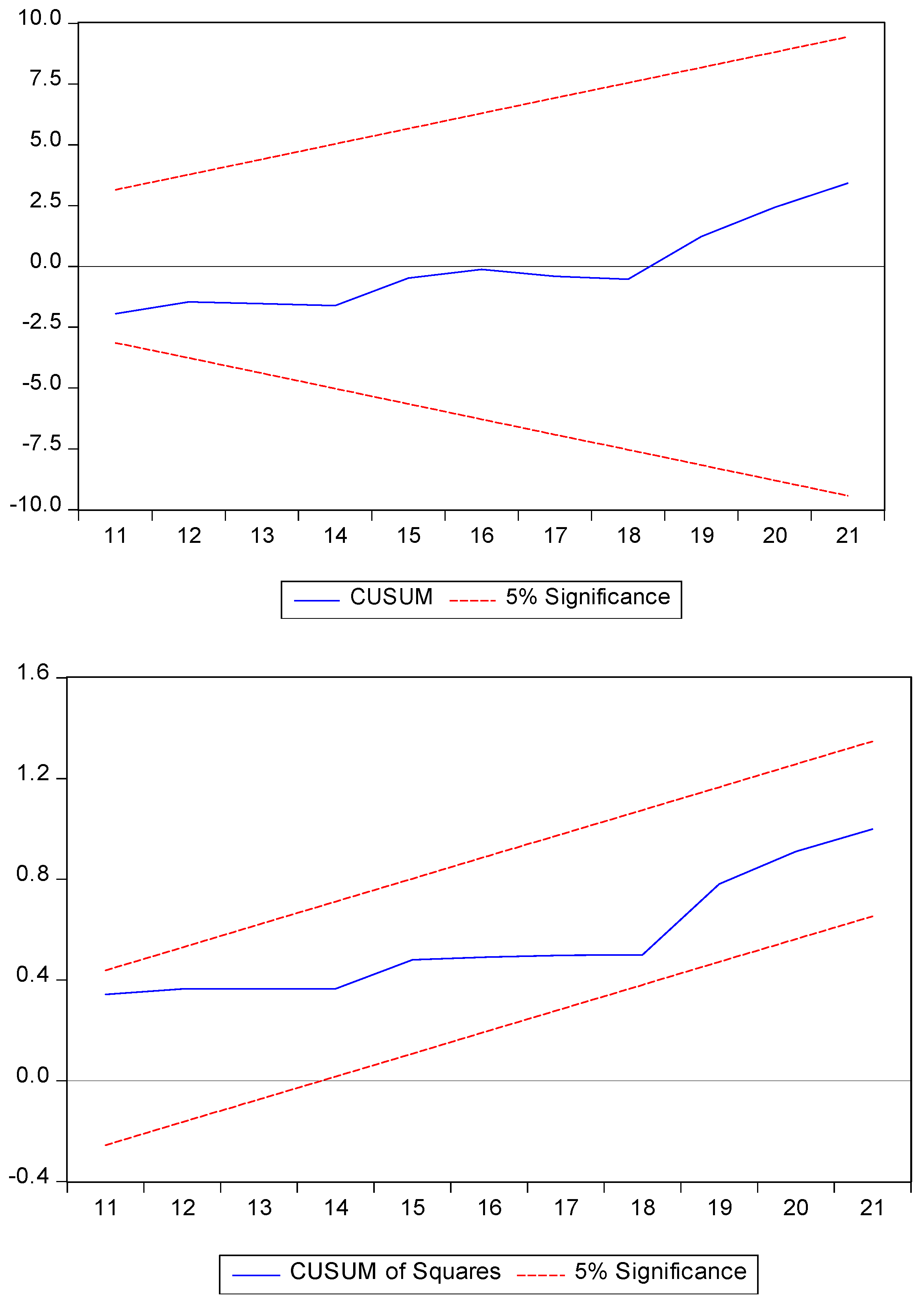
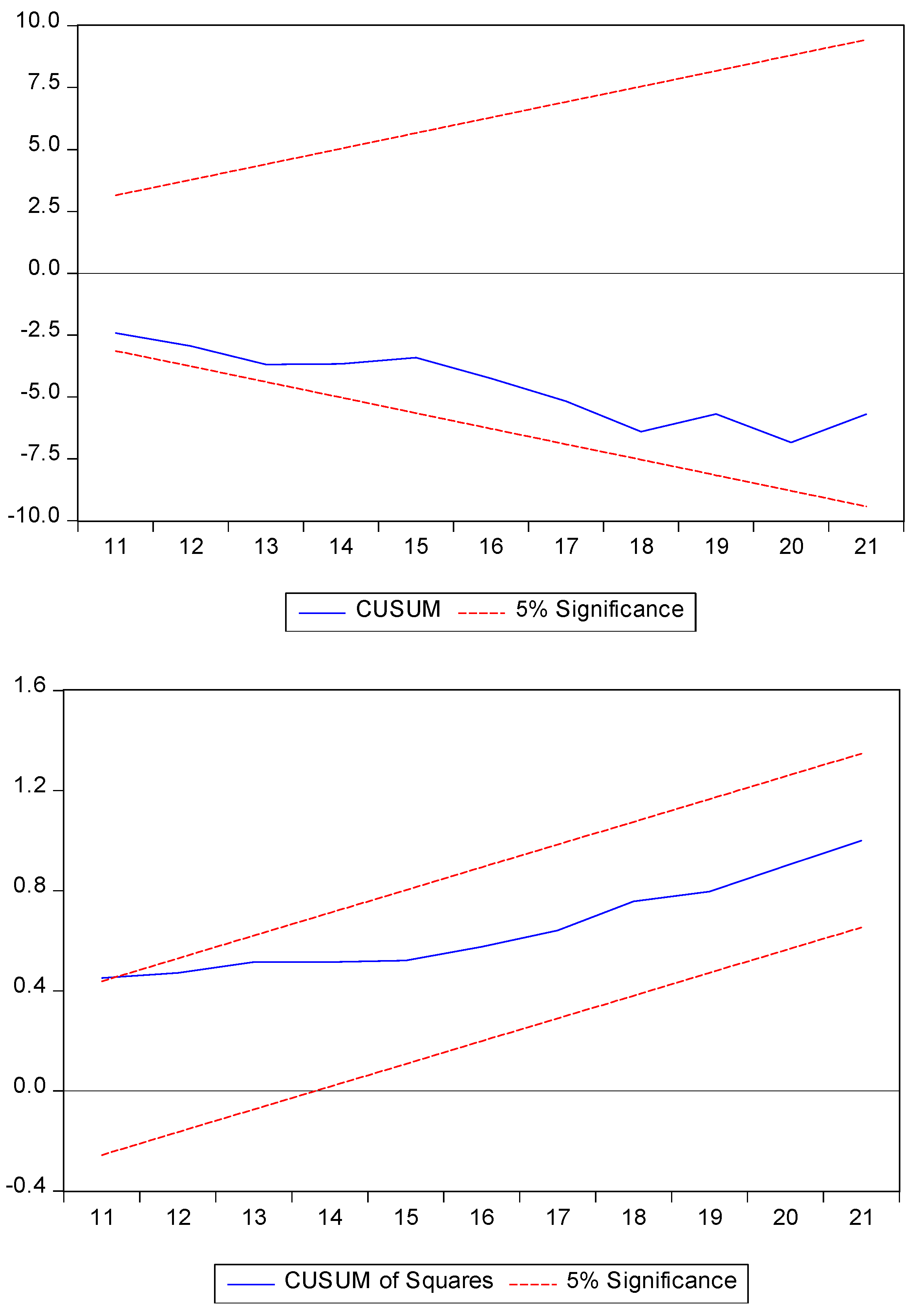
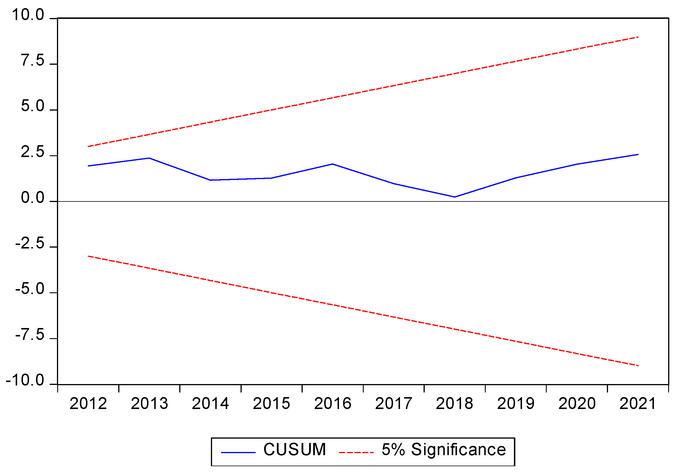
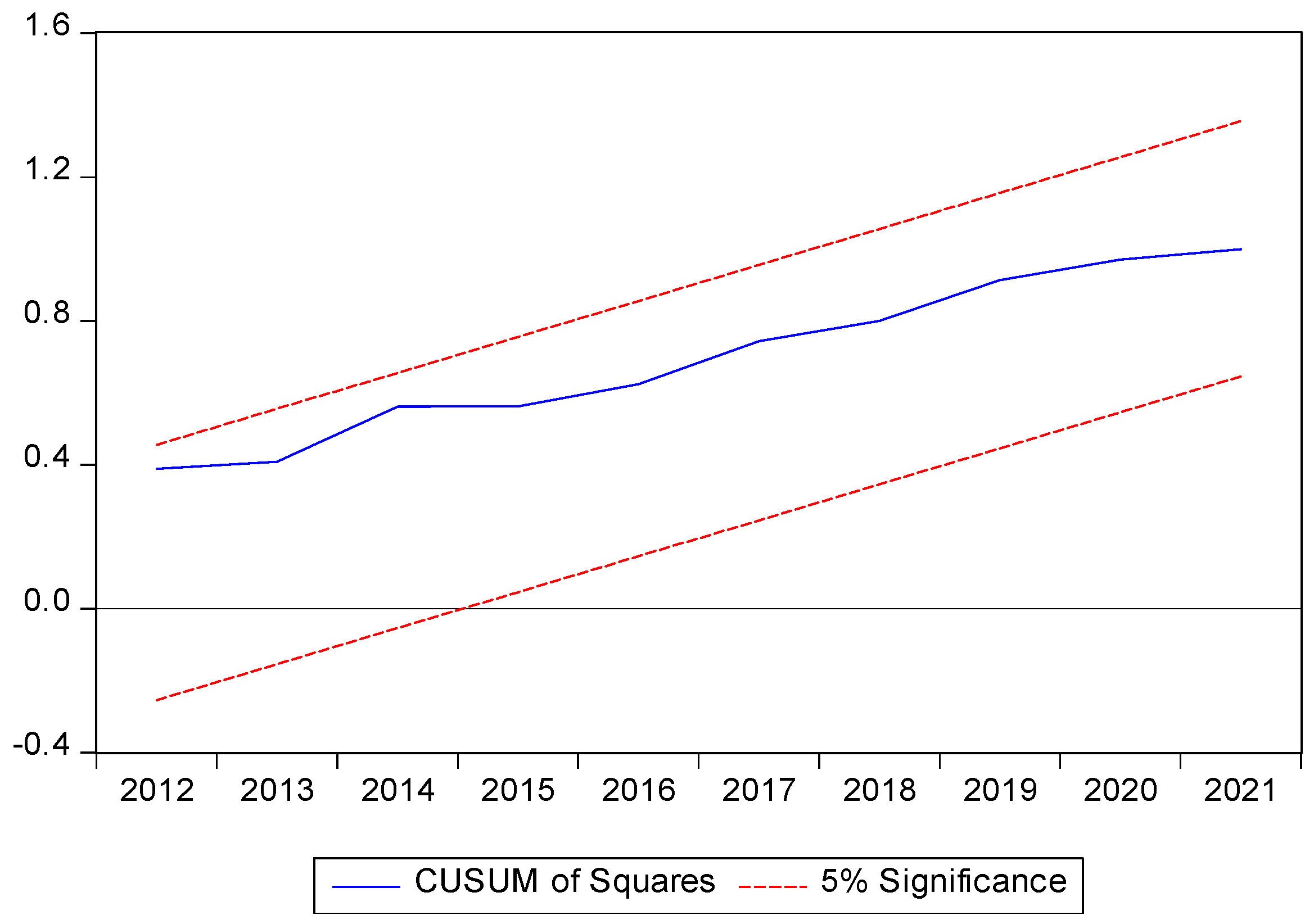
In addition to Ramsey RESET Test, the study used both the CUSUM test and the CUSUM of the square test as a recursive estimator (Brown et al. 1975) to further check for the goodness-of-fit and the stability of the ARDL model (Pesaran and Shin 1995). Figure 1 demonstrates the CUSUM and CUSUM of squares for Model 1. Figure 2 represents the CUSUM and CUSUM of Squares for Model 2. Figure 3 exhibits the CUSUM and CUSUM of Squares for Model 3. Figure 1, Figure 2 and Figure 3 demonstrate that the three models are a good fit as their lines lie between the 5% significance boundaries.

5. Conclusions and Policy Implications

The study on the determinants of the CAR of Jordanian banks identified several variables that significantly affect the CAR in both the short and the long run. In the short run, the study found that banks’ credit to-deposits ratio, banks’ leverage ratio, banks’ liquidity ratio, one-year-lagged ROE, capital-to-assets ratio, one-year-lagged capital asset ratio, LATD, and coverage ratio significantly affect the CAR of Jordanian banks.

In the long run, the results suggest the leverage ratio (LEVR), liquidity ratio (LIQR), capital-to-assets ratio (CTA), and liquid-assets-to-deposits ratio (LATD) significantly affect the CAR of Jordanian banks.

According to the pairwise Granger causality method, LATD is shown to granger cause the CAR at a 1% level of significance, and money supply (M2), ROE, and capital to assets ratio (CTA) all granger cause the CAR at a 0.05 level of significance. The CAR in Jordanian banks was shown to be statistically less relevant to the remaining factors. The models used in the study were homoscedastic, stable, serial correlation free, and ARCH effect free, and their residuals are normally distributed. The study’s findings highlight the significance of comprehending the variables’ effects on the CAR, including their direction and magnitude.

The study on the determinants of the CAR of Jordanian banks, using an ARDL bound testing approach, provides important policy implications for the banking sector in Jordan. The findings indicate that several variables significantly affect the CAR of Jordanian banks, including banks’ credit to-deposits ratio, banks’ leverage ratio, banks’ liquidity ratio, one-year-lagged ROE, capital-to-assets ratio, one-year-lagged capital-to-asset ratio, LATD, and coverage ratio.

In the short run, the study found that banks’ credit to-deposits ratio, banks’ leverage ratio, banks’ liquidity ratio, one-year-lagged ROE, capital to assets ratio, one-year-lagged capital asset ratio, LATD, and coverage ratio significantly affect the CAR of Jordanian banks. In addition, the results suggest the leverage ratio (LEVR), liquidity ratio (LIQR), capital-to-assets ratio (CTA), and LATD significantly impact the CAR of Jordanian banks in the long run.

The policy implications of these findings are twofold. Firstly, policymakers in Jordan need to focus on the importance of economic growth and stability as a means to increase the CAR of Jordanian banks. They should encourage policies that promote economic growth and stability, such as improving the business environment and promoting financial stability.

Secondly, policymakers should also address the liquidity risk and profitability of Jordanian banks, which are identified as important determinants of the CAR. To enhance liquidity risk management, policymakers should ensure that banks have access to diversified sources of funding, and they should encourage banks to maintain adequate liquidity buffers. To improve profitability, policymakers should promote competition and innovation in the banking industry, as well as support financial inclusion and access to credit for small- and medium-sized businesses.

Policymakers and regulators need to ensure that the banking sector is adequately capitalized by setting appropriate regulatory standards for the CAR. This can help to safeguard the stability and resilience of the banking sector, particularly during times of economic stress.

Overall, this study highlights the importance of sound macroeconomic policies, effective risk management practices, and a competitive and innovative banking sector in enhancing the CAR of Jordanian banks. These policy implications can also be relevant to other developing economies that face similar challenges in maintaining a stable and well-capitalized banking sector.

6. Scope and Limitation of the Study

Understanding the determinants of the CAR is crucial for ensuring the stability of the banking sector and, ultimately, the overall economy. The study provides evidence to the research community of how certain firm-specific variables and macroeconomic variables influence the CAR of Jordanian banks. The study offers valuable insights into the factors influencing the capital adequacy ratio of the Jordanian banking sector. However, it is important to acknowledge certain limitations within the study. Firstly, the research focuses solely on the Jordanian banking sector, which limits the generalizability of the findings to other countries or regions. Additionally, the study employs an autoregressive distributed lag-bound testing approach, which may have inherent assumptions and limitations. With a limited data series, it becomes challenging to capture the full range of variations and dynamics within the variables over time.

Overall, while the study provides valuable insights, these limitations should be taken into consideration when interpreting the results and applying them to real-world scenarios. Future research on exploring the impact of the CAR on the overall financial strength of Jordan could be a valuable area of study.