Durable Consumption-Based Asset Pricing Model with Foreign Factors for the Korean Stock Market

Abstract

This paper explores the implications of consumption heterogeneity between domestic and foreign investors on the cross-section of stock returns in a host country. We argue that foreign investors in a small open economy integrated into global financial markets may face consumption risk, which could result in risk premia being reflected in stock returns. To account for the potential influence of foreign investors on asset prices in a host country, we develop a two-country durable consumption model under market incompleteness, which extends the one-country durable consumption model. The proposed model includes both domestic and foreign pricing factors. We investigate the empirical performance of our model with Fama–French portfolios for Korea, taking U.S. investors as representative foreign investors. The empirical results advocate the two-country durable consumption model, confirming the significant role of foreign factors in the cross-section of domestic stock returns. Additionally, $R^2$ tests conducted with different sets of test assets show that the explanatory power of our model is comparable to that of the Fama–French three-factor model.

1. Introduction

The influence of foreign investors on host countries has been studied from various perspectives. One area of research investigates the effects of integration with global financial markets on local economies and financial markets. Chari and Henry (2004) found that the access of foreign investors to local stock markets lowers systematic risk and leads to the revaluation of stocks in a host country. Bekaert et al. (2005) argued that financial liberalization can promote economic growth through foreign financial flows. They argued that as foreign investors supply funds and improve corporate governance, liberalized financial markets contribute to the decrease in the cost of capital and the increase in physical investment in a host country.

On the other hand, many studies address the problems that foreign investors can bring to host countries. For example, Bae et al. (2004) suggested that stocks attracting foreign investors in emerging countries are more exposed to world market risk and, therefore, experience higher volatility. Furthermore, Stiglitz (2004) claimed that foreign financial flows could increase macroeconomic volatility. Debates are, however, still ongoing. Using Korean data, Choe et al. (1999) found no evidence to show that foreign investors destabilize stock markets. In addition, Umutlu et al. (2010) found stronger results, which showed that as financial liberalization broadens the base of investors, foreign investment reduces the volatility of stock returns in emerging countries.

Another important area of the literature explores the effects of foreign investors’ participation on asset prices. This area of research mainly focuses on information asymmetry between local and foreign investors. Chan et al. (2008) presented interesting results, which suggested that information asymmetry in the Chinese stock market has led to a large discount for B-shares.1 Regarding stock market expectations, Brennan et al. (2005) found that when foreign investors have informational disadvantages, they are more likely to have pessimistic views after a rise in the stock market of the host country. Brennan and Cao (1997) suggested that the stock purchases of foreign investors tend to be positively related to returns if they are less informed.

The present paper also investigates the role of foreign investors in asset prices. However, rather than information heterogeneity, we focus on the importance of consumption heterogeneity in the context of a cross-section of stock returns. As is commonly known, there is a unique stochastic discount factor (SDF) in a complete market. In this case, using the SDF of local households will be equivalent to using that of foreign households in pricing the assets of a host country. However, in an incomplete market, where foreign and domestic SDFs are not identical, the former can have additional information content for pricing assets. Based on this idea, we explore whether heterogeneity in consumption between host and foreign countries plays a significant role in explaining stock returns in the host country under the assumption of market incompleteness. To this end, we extend the durable consumption model of Yogo (2006) to a two-country setting by including the consumption factors of a foreign country in our domestic pricing model.

To investigate the empirical performance of our model, we used Korean stock market data. Foreigners’ stock investment2 was fully liberalized in May 19983, resulting in consistently large holdings of Korean stocks by foreign investors. Figure 1a shows the shares held by foreign investors in the Korean stock markets (KOSPI and KOSDAQ). On average, foreign investors held one-third of the market value during the 2001–2016 period. In addition, Figure 1b shows the composition of foreign investors by nationality, with U.S. and U.K. investors being the largest two investor groups. Over the 2001–2016 period, U.S. investors were the dominant group, accounting for an average of 44% of all foreign investment, whereas U.K. investors accounted for only around 11% during the same period.

These descriptive statistics imply that U.S. investors may have a non-trivial influence on the Korean stock market, as foreign investors collectively play a considerable role. Motivated by these ideas, we believe that the Korean stock market serves the goal of our empirical study. In particular, the presence of the dominant investor group enables us to estimate the model in a relatively parsimonious way without much loss of information. Anticipating this benefit, we adopt the SDF of the U.S. as a representative SDF for foreign investors.

The main contributions and findings of this paper are as follows. We construct a two-country linear factor model that includes domestic (Korea) and foreign (U.S.) factors. Using a variety of test assets, including Fama–French and industry portfolios, we estimate the model and show that the risk factors implied by the U.S. investors’ SDF are jointly significant. Moreover, when portfolios with low book-to-market (BE/ME) ratios are excluded from the test assets, most of the individual domestic and foreign consumption risk factors are significantly priced. This result suggests that a small open economy integrated into global financial markets has important asset pricing implications. In principle, stocks that earn higher (lower) returns in good (bad) times are considered riskier so investors require higher risk premia for these stocks. In the consumption-based asset pricing framework, these good times are when marginal utility falls, that is, when consumption grows. If there is an investor group holding a large share in a stock market, stock returns will contain risk premia for the consumption risk faced by the investor group. Our findings suggest that as foreign investors hold a substantial share of the market in Korea, stocks in the host country compensate for their risk-bearing. In particular, the compensation of Korean stocks is robust for durable consumption risk in the U.S. across all the samples we considered. Thus, this result implies that U.S. durable consumption cycles need to be taken into account when pricing Korean stocks.

In model comparisons, the Fama–French three-factor model outperformed the two-country durable consumption model for 25 Fama–French, and 25 Fama–French plus 8 industry portfolios. However, we found that the inclusion of industry portfolios adversely affected the three-factor model more than our model. Furthermore, according to formal tests by Kan et al. (2013), the explanatory power of our model was comparable to that of the Fama–French three-factor model for most of the samples we considered.

Our empirical results highlight the significance of cross-country heterogeneity in consumption for explaining asset prices in countries such as Korea, where the share of foreign investors is large. However, despite its potential importance, consumption heterogeneity across countries has received relatively little attention in the asset pricing literature. Exceptions include Sarkissian (2003), Li and Zhong (2005), and Darrat et al. (2011). Similar to Constantinides and Duffie (1996), Sarkissian (2003) incorporates cross-country consumption heterogeneity into his model. However, the primary goal of his paper is to explain currency risk premia and cross-sectional differences in currency returns, not stock returns. In this sense, our work is more closely related to those of Li and Zhong (2005) and Darrat et al. (2011). Li and Zhong (2005) examined the predictability of country-level stock returns in relation to consumption heterogeneity. Darrat et al. (2011) considered consumption heterogeneity in order to explain the cross-section of country-level stock returns. Compared with the two studies above, our work differs in that we focus on the cross-section of domestic stock returns, whereas those authors studied aggregate stock returns across countries and although they modeled consumption heterogeneity with cross-sectional consumption dispersion as in Constantinides and Duffie (1996), we reflected on it more directly by using the SDF of a dominant foreign investor. Our model builds on the durable consumption model of Yogo (2006) that adopts the Epstein–Zin preferences, whereas existing studies employ the standard power utility (Li and Zhong 2005) or habit-based (Darrat et al. 2011) models.

The rest of this paper is organized as follows. In Section 2, we present a durable consumption model for empirical analysis. Section 3 describes the data for the estimation. In Section 4, we discuss the estimation results. Section 5 concludes the paper. Additional estimation results are provided in Appendix A.

2. Model

This section describes the setup of the two-country consumption model and derives a linear factor representation for the expected excess return. The economy consists of households in two countries—home and foreign—and a firm in the home country. As in Yogo (2006), households consume both durable and non-durable goods. In addition, the representative firm maximizes its value subject to a weighted average of the SDFs of the households in the two countries.

2.1. Households

The households in the two countries have Epstein–Zin preferences4, where they gain utility from non-durable and durable goods consumption. Since the households’ problems are almost identical, except for the adjustment for returns on foreign assets due to the real exchange rate, we state the problem for the households in the home country only. This description is sufficient to derive the econometric specifications without overlooking the key features of our model.

In the economy, households consume non-durable goods and service flows from durable goods. As in Colacito and Croce (2011), we assume that households in one country only consume goods produced in their own country. Non-durable goods ($C_t$) are standard consumption goods that are completely consumed within a period. However, durable consumption goods ($D_t$) are accumulated as stock and can provide service flows to households over a long period of time. The law of motion for the stock of durable goods is given by

$$\begin{array}{c}\hfill D_t=(1-\delta )D_{t-1}+E_t,\end{array}$$

(1)

where $E_t$ is the durable goods consumption expenditure and $\delta$ is the depreciation rate.

We assume that households have Epstein–Zin preferences, including both non-durable and durable consumption

$$\begin{array}{c}\hfill U_t={\left\{(1-\beta )u{(C_t,D_t)}^{1-1/\psi }+\beta E_t{\left[U_{t+1}^{1-\gamma }\right]}^{\frac{1-1/\psi }{1-\gamma }}\right\}}^{\frac{1}{1-1/\psi }},\end{array}$$

(2)

where $\psi$ is the intertemporal elasticity of substitution (IES) and $\gamma$ is the coefficient of relative risk aversion. $u(C_t,D_t)$ denotes the household’s intraperiod utility, which has the following CES form:

$$\begin{array}{c}\hfill u(C_t,D_t)=\left\{(1-\alpha )C_t^{1-1/\rho }+\alpha D_t^{1-1/\rho }\right\},\end{array}$$

(3)

where $\rho$ is the elasticity of substitution between non-durable and durable consumption goods and $\alpha$ is the utility weight of durable consumption.

Households invest ${\theta }_{i,t}$ units of wealth in asset i. Then, the budget constraint is given by

$$\begin{array}{c}\hfill \sum _{i=1}{\theta }_{i,t}=W_t-C_t-P_t{E}_t,\end{array}$$

(4)

where $W_t$ is the household’s wealth and $P_t$ is the price of the durable good. The household’s wealth in the next period is given by

$$\begin{array}{c}\hfill W_{t+1}=\sum _{i=1}{\theta }_{i,t}{R}_{i,t+1},\end{array}$$

(5)

where $R_{i,t+1}$ is the real return for asset i. Note that the return is measured in consumption units of the household’s home country, as we allow investment in both foreign assets and home assets.

Letting $R_{W,t+1}$ be the return on wealth, we can derive the SDF from the household’s problem as follows:

$$\begin{array}{c}\hfill M_{t+1}={\left[\beta {\left(\frac{C_{t+1}}{C_t}\right)}^{-1/\psi }{\left(\frac{v(D_{t+1}/C_{t+1})}{v(D_t/C_t)}\right)}^{1/\rho -1/\psi }{R}_{W,t+1}^{1-\kappa }\right]}^{\kappa },\end{array}$$

(6)

where $\kappa =(1-\gamma )/(1-1/\psi )$ and $v(D/C)$ is defined by

$$\begin{array}{c}\hfill v\left(\frac{D}{C}\right)={\left[1-\alpha +\alpha {\left(\frac{D}{C}\right)}^{1-1/\rho }\right]}^{1/(1-1/\rho )}.\end{array}$$

(7)

Now, we distinguish between the SDF of domestic households and that of foreign households by denoting them as $M_{1,t+1}$ and $M_{2,t+1}$, respectively. The domestic household’s Euler equation for home equity j is then

$$\begin{array}{c}\hfill 1=E_t\left[M_{1,t+1}{R}_{j,t+1}\right],\end{array}$$

(8)

where $R_{j,t+1}$ is the gross return in terms of the home country’s consumption units. Finally, the foreign household’s Euler equation for the same equity j is given by

$$\begin{array}{c}\hfill 1=E_t\left[M_{2,t+1}\frac{e_t}{e_{t+1}}{R}_{j,t+1}\right].\end{array}$$

(9)

Note that the real return (in terms of the foreign country’s consumption unit) for foreign investors is $\frac{e_t}{e_{t+1}}{R}_{j,t+1}$, where the real exchange rate is the relative price of foreign consumption goods in terms of domestic consumption goods.5

2.2. Firms

The representative firm maximizes its value, which is the sum of the discounted dividend flows ($d_t$). We assume a typical firm, as specified in Kaltenbrunner and Lochstoer (2010), Croce (2014), and many others. The firm value ($V_t$) is defined by

$$\begin{array}{c}\hfill V_t=d_t+E_t\left[M_{t+1}^{*}{V}_{t+1}\right],\end{array}$$

(10)

where $M_{t+1}^{*}$ is the SDF of the stockholders. Here, the stock return is given by

$$\begin{array}{c}\hfill R_{t+1}=\frac{V_{t+1}}{V_t-d_t},\end{array}$$

(11)

where $V_{t+1}$ is the cum-dividend firm value at $t+1$ and $V_t-d_t$ is the ex-dividend firm value at t. By combining Equations (10) and (11), we obtain the Euler equation for the firm:

$$\begin{array}{c}\hfill 1=E_t\left[M_{t+1}^{*}{R}_{t+1}\right].\end{array}$$

(12)

In the model, the households in the two countries are stockholders of the firm. As suggested by Fogli and Perri (2015), we assume that the firm maximizes its value with the weighted average of the stochastic discount factors of the households in the two countries. We use the geometric average of the SDFs, similar to Eyster et al. (2019).6 Then, the SDF ($M_{t+1}^{*}$) in the firm’s problem is given by

$$\begin{array}{c}\hfill M_{t+1}^{*}=M_{1,t+1}^{1-\omega }{\left(M_{2,t+1}\frac{e_t}{e_{t+1}}\right)}^{\omega },\end{array}$$

(13)

where $M_{i,t+1}$ is the SDF of the household in country i and $\omega$ is the weight of foreign stockholders. In a complete market, the following result will hold for all states7,

$$\begin{array}{c}\hfill M_{t+1}^{*}=M_{1,t+1}=M_{2,t+1}\frac{e_t}{e_{t+1}}.\end{array}$$

(14)

However, in an incomplete market, the equality in Equation (14) breaks down and the SDF is given as in Equation (13).

2.3. The Two-Country Linear Factor Model

Yogo (2006) showed that the Euler equation of the durable consumption model (with a single country) can be approximated by a linear factor model. We follow his framework to derive a linear factor representation in a two-country setting. As in Yogo (2006), we apply the first-order log-linear approximation to the firm’s SDF $M_{t+1}^{*}$ to obtain

$$\begin{array}{c}\hfill \frac{M_t^{*}}{E\left[M_t^{*}\right]}\simeq 1+m_t^{*}-E\left[m_t^{*}\right],\end{array}$$

(15)

where $M_t^{*}={\left(M_t^{KR}\right)}^{(1-\omega )}{\left(M_t^{US}\frac{e_{t-1}}{e_t}\right)}^{\omega }$, $m_t^{*}=log{M}_t^{*}=(1-\omega )m_t^{KR}+\omega m_t^{US}$, and $m_t^{KR}$ and $m_t^{US}$ are the logarithms of the SDFs for the Korean and U.S. households, respectively.

By taking a log-linear approximation, one can show that the SDF for a Korean household is approximated as

$$\begin{array}{cc}\hfill & -m_t^{KR}\simeq -{\kappa }^{KR}log{\beta }^{KR}+B_1\Delta c_t^{KR}+B_2\Delta d_t^{KR}+B_{3}r{w}_t^{KR},\hfill \end{array}$$

(16)

where $\Delta c_t^{KR}$ and $\Delta d_t^{KR}$ are, respectively, non-durable and durable consumption growth in Korea, and $r{w}_t^{KR}$ is the return on wealth for the Korean household. Similarly, the SDF for a U.S. household is given by

$$\begin{array}{cc}\hfill & -m_t^{US}\simeq -{\kappa }^{US}log{\beta }^{US}+B_4\Delta c_t^{US}+B_5\Delta d_t^{US}+B_{6}r{w}_t^{US}.\hfill \end{array}$$

(17)

By combining Equations (12), (15), (16), and (17), the following linear factor representation can be derived8

$$\begin{array}{cc}\hfill & E[R_{i,t}-R_{f,t}]\hfill \\ \hfill & =b_{1}Cov(\Delta c_t^{KR},R_{i,t}-R_{f,t})+b_{2}Cov(\Delta d_t^{KR},R_{i,t}-R_{f,t})+b_{3}Cov(r{w}_t^{KR},R_{i,t}-R_{f,t})\hfill \\ \hfill & +b_{4}Cov(\Delta c_t^{US},R_{i,t}-R_{f,t})+b_{5}Cov(\Delta d_t^{US},R_{i,t}-R_{f,t})+b_{6}Cov(r{w}_t^{US},R_{i,t}-R_{f,t})\hfill \\ \hfill & +b_{7}Cov(\Delta e_t,R_{i,t}-R_{f,t}),\hfill \end{array}$$

(18)

where $R_{f,t}$ and $R_{i,t}-R_{f,t}$ are the risk-free rate and the excess return of portfolio i, respectively. $\Delta c_t^j$ and $\Delta d_t^j$ are the non-durable and durable consumption growth in country j. $r{w}_t^j$ is the return on wealth in country j. $\Delta e_t$ is the change in the real exchange rate, which captures changes in the nominal exchange rate and inflation differentials between Korea and the U.S.9 Here, $b_7=\omega$ is the weight of the U.S. households. The other coefficients $b_m$s are defined as follows:

$$b_m=\left\{\begin{array}{ll}\left(1-\omega \right)B_m& \mathrm{for}1\le m\le 3\hfill \\ \omega B_m& \mathrm{for}4\le m\le 6\hfill \end{array}\right.$$

Yogo (2006)’s one-country durable consumption model (1C EZ-D) is nested in our model with the restriction of $b_4=b_5=b_6=b_7=0$. Other conventional one-country consumption-based models and their extensions to a two-country setting are all special cases of our model, with the following parameter restrictions:

• $b_2=b_4=b_5=b_6=b_7=0$: Non-durable consumption Epstein–Zin CAPM (1C EZ-ND),
• $b_2=b_3=b_4=b_5=b_6=b_7=0$: Power utility CCAPM (1C Power),
• $b_2=b_5=0$ and $b_7\ne 0$: Two-country non-durable Epstein–Zin (2C EZ-ND),
• $b_2=b_3=b_5=b_6=0$ and $b_7\ne 0$: Two-country power utility (2C Power).

Note that the factors related to U.S. households only appear in the SDFs for our model and specifications 3 and 4 above.

3. Data

In this section, we provide data descriptions for the test assets and pricing factors.

3.1. Portfolio Data

Following Fama and French (1993), we constructed $5\times 5$ sized (ME) and book-to-market (BE/ME) portfolios. We used the KISVALUE database, which provides stock return and accounting data for portfolio construction. Our data included all non-financial KOSPI (Korean Composite Stock Price Index) and KOSDAQ (Korean Securities Dealers Automated Quotations) firms that traded on the Korean Exchange during the 2001–2015 period.

For the construction of the size portfolios, we used the market equity of each firm, which is defined as its stock price times the shares outstanding. Then, the size of the firm was measured by its market equity as of June of each year. After five size portfolios were formed, they were rebalanced in July of the following year. To form the book-to-market equity portfolios, the book equity of each firm was computed as the book value of its assets minus its total liabilities using balance sheets. The market equity for the book-to-market equity sorts was measured by the value at the end of December in the previous year. Like the size portfolios, the book-to-market equity portfolios were rebalanced in July of the following year. In both the size and book-to-market equity portfolios, firms with negative book equity were excluded. The quarterly excess returns of each portfolio were computed as the value-weighted return of a portfolio minus the 91-day CD (certificate of deposit) rate.

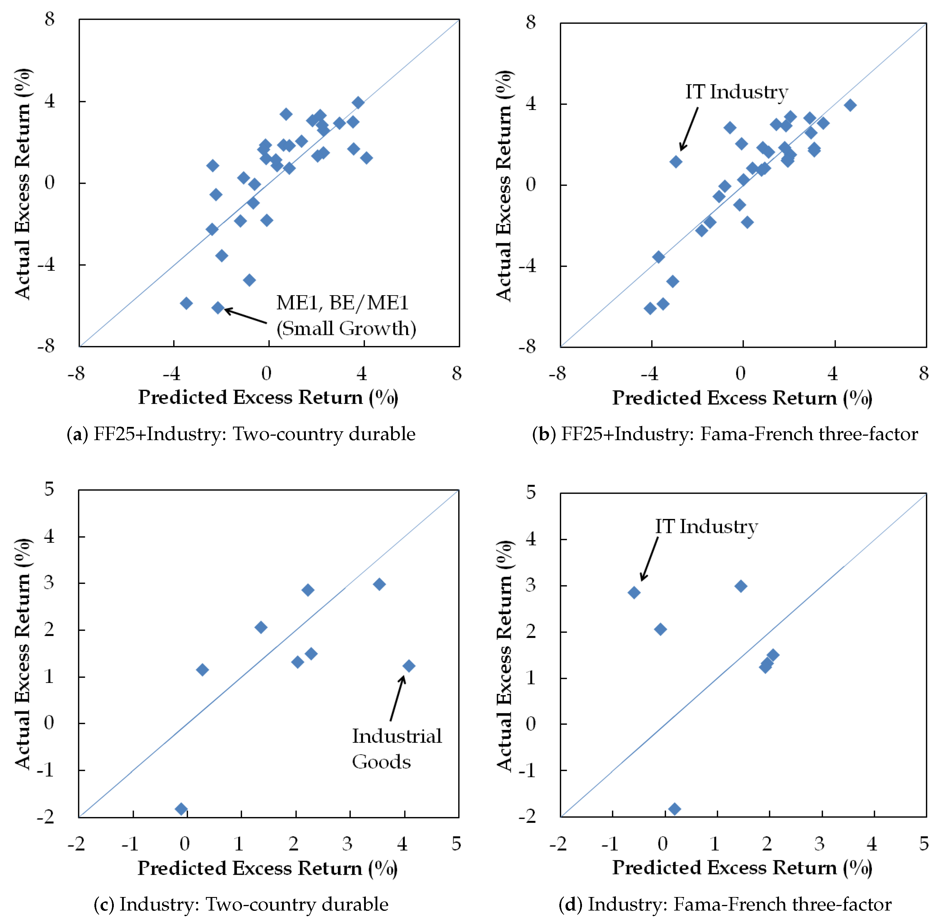
3.2. Macroeconomic Data for Factors

We used quarterly macroeconomic data for Korea and the U.S. for the period 2001–2015. The macroeconomic data required for the estimation were the non-durable goods and services consumption, durable goods consumption, and returns on wealth in the two countries. Using expenditure data for individual items from the Household Income and Expenditure Survey conducted by Statistics Korea (the national statistical agency), we computed the aggregate durable and non-durable consumption, with the classifications consistent with those used by Yogo (2006). Major non-durable consumption items include food and beverages, clothing and shoes, housing, healthcare services, and transportation. For non-durable and durable consumption in the U.S., we used data compiled by the Bureau of Economic Analysis (BEA).

As mentioned in Section 2.1, since households consume service flows from a durable good for a long period of time, we needed to estimate the stock of durable goods. We constructed the series assuming the law of motion for the stock of a durable good ($D_t$) specified by Equation (1). In particular, following the methodology of Yogo (2006), we used $\delta =0.06$ as the quarterly depreciation rate for both countries. The initial value $D_0$ was estimated by $D_0=\frac{E_1}{g+\delta }$, where g is the mean growth rate in durable goods consumption expenditure ($g=0.011$ in Korea for 1990–2016 and $g=0.010$ in the U.S. for 1947–2016).

In addition to consumption data, our durable consumption model includes returns on wealth. Following the methodology of Campbell (1996), Lustig and Van Nieuwerburgh (2008), and Jeong et al. (2015), we included returns on human wealth, as well as those on financial wealth from stocks.10 Here, returns on human wealth are represented by the growth rate of labor income, which consists of employee compensation and proprietors’ income. We computed the total return on wealth using a weight of 0.7 for human wealth. Our weight is the mean value of 0.73 from Campbell (1996) and 0.66 from Jeong et al. (2015).

Lastly, for real exchange rate adjustments, we used the nominal exchange rates at the end of each quarter, which are available from the Bank of Korea. The inflation rates were calculated using the CPIs for Korea and the U.S.

3.3. Summary Statistics

Table 1. Average returns on 25 Fama–French Portfolios.

ME	BE/ME					Average
	1 Low	2	3	4	5 High
1 Small	−0.060	0.020	0.007	0.029	0.047	0.009
2	−0.036	−0.013	−0.003	0.021	0.042	0.002
3	−0.052	−0.011	0.005	0.023	0.037	0.001
4	−0.028	−0.002	0.015	0.034	0.043	0.012
5 Big	0.013	0.024	0.024	0.035	0.022	0.024
Average	−0.033	0.004	0.010	0.028	0.038

This table presents the average returns for each Fama–French portfolio. Following the methodology of Fama and French (1993), we assigned individual stocks to size and book-to-market groups based on quintile breakpoints. We computed quarterly returns using monthly stock price data provided by KISVALUE for 2001–2015.

shows the average excess returns for the Fama–French portfolios, where it can be seen that there exists both a similarity and a difference between Korea and the U.S. in the cross-section of stock returns. Fama and French (1992) reported a positive relationship between book-to-market and average returns for U.S. data. Similar to Fama and French (1992), we found that higher book-to-market portfolios had larger average excess returns11 in Korea. The last row in the table highlights this fact. In addition, for each size group, the excess returns based on the BE/ME sorts exhibited a general tendency that coincided with the results of Fama and French (1992). On the other hand, we did not find a negative relationship between size and average returns, unlike Fama and French (1992) for U.S. data. The average return in Table 1 shows a U-shaped pattern as the size increases, as seen in the last column, The table also indicates that, on average, large firms (ME 4 and ME 5) pay higher excess returns than small firms. Although Yun et al. (2009) found a negative relationship in the Korean data, their sample period (1991–2007) differed from ours (2001–2015). Thus, the size–return relationship in Fama–French (1992) may be country- and time-specific.

Table 2. Descriptive statistics.

	$C^{KR}$	$D^{KR}$	$R_w^{KR}$	$C^{US}$	$D^{US}$	$R_w^{US}$	$Market$	$HML$	$SMB$
Mean (%)	0.175	1.052	1.119	0.219	1.042	0.478	1.186	6.981	−1.825
SD (%)	1.490	0.865	0.346	0.517	3.659	2.910	11.728	7.906	11.742
	Correlations
$C^{KR}$
$D^{KR}$	−0.030
$R_w^{KR}$	0.153	0.115
$C^{US}$	0.207	−0.045	0.259
$D^{US}$	0.170	−0.009	0.232	0.660
$R_w^{US}$	0.207	0.082	0.621	0.402	0.077
$Market$	0.284	0.040	0.973	0.063	0.093	0.618
$HML$	0.153	−0.040	−0.133	0.009	0.209	−0.157	−0.164
$SMB$	−0.023	0.156	−0.083	−0.021	−0.133	−0.085	−0.050	−0.694

This table presents the descriptive statistics for the key macroeconomic data. The first two rows show the means and standard deviations. The remaining rows show the correlations between the variables. $C^i$, $D^i$, and $R_w^i$ denote non-durable consumption, durable consumption, and the return on wealth in country i, respectively. $Market$ represents the excess return for the market portfolio (KOSPI and KOSDAQ) in Korea. $SMB$ is the difference in the average returns between the small stock and big stock portfolios. $HML$ is the difference in the average returns between the high book-to-market equity and low book-to-market equity portfolios. The superscripts $KR$ and $US$ represent Korea and the U.S., respectively. All numbers are quarterly values.

presents descriptive statistics of our key variables used in the estimation. The first two rows show that the mean growth rates of both durable and non-durable consumption were similar in both countries, whereas the standard deviations were quite different. Non-durable consumption was more volatile in Korea than in the U.S., whereas durable consumption was more volatile in the U.S. Table 2 also shows that the correlation of consumption growth was weak between the two countries. For non-durable goods, the correlation coefficient between them was only 0.207 and it was even smaller for durable consumption (−0.009). In addition, the correlations between Korea and the U.S. were also low across different consumption categories (non-durable in Korea and durable in the U.S.: 0.170; durable in Korea and non-durable in the U.S.: −0.045). The substantial consumption heterogeneity across the two countries suggests that the stochastic discount factor of the U.S. households could provide independent information for pricing assets.

4. Cross-Sectional Test of the Two-Country Durable Consumption Model

In this section, we estimate the two-country linear factor model given in Equation (18). We call this linear factor model the “two-country durable consumption model”. The estimation results of our model are compared to those of the traditional CAPM, the restricted versions of our two-country durable consumption-based model, and the Fama–French three-factor model.

4.1. Estimation of the Two-Country Durable Consumption Model

We estimate the model parameters using the generalized method of moments (GMM). Since the moment condition is given by $E\left[M_t^{*}(R_{i,t}-R_{f,t})\right]=0$ for each portfolio i, the number of moment conditions is equal to that of the test assets, n. Let $R_t$ be the vector of portfolio returns and $f_t$ be the de-meaned vector of factors at time t. Then, the moment function from Equation (18) is given by

$$\begin{array}{c}\hfill g(x_t,b)=\left(R_t-R_{f,t}\iota -(R_t-R_{f,t}\iota )f_t^{\prime }b\right),\end{array}$$

(19)

where $x_t=(R_{f,t},R_{1,t},\dots ,R_{n,t})$ and $\iota$ is an $n\times 1$ vector of ones. b is the vector of coefficients in the linear factor model.

We estimate the model using a two-stage GMM. Let W and $g_T$ denote a weighting matrix and the sample moment, respectively. Then, the GMM estimator minimizes the weighted sum of pricing errors:

$$\begin{array}{c}\hfill mi{n}_b{J}_T=g_T^{\prime }W{g}_T,\end{array}$$

(20)

where $g_T=\frac{1}{T}{\sum }_{t=1}^T\left[R_t-R_{f,t}\iota -(R_t-R_{f,t}\iota )f_t^{\prime }b\right]$. The first stage uses an identity weighting matrix, which weights all moment conditions equally. Then, we compute a heteroscedasticity and autocorrelation consistent (HAC) estimate of the covariance matrix of the pricing errors $g_T$. In the second stage, the inverse of this covariance matrix is used as the weighting matrix, which yields efficient estimates.

4.2. Estimation Results

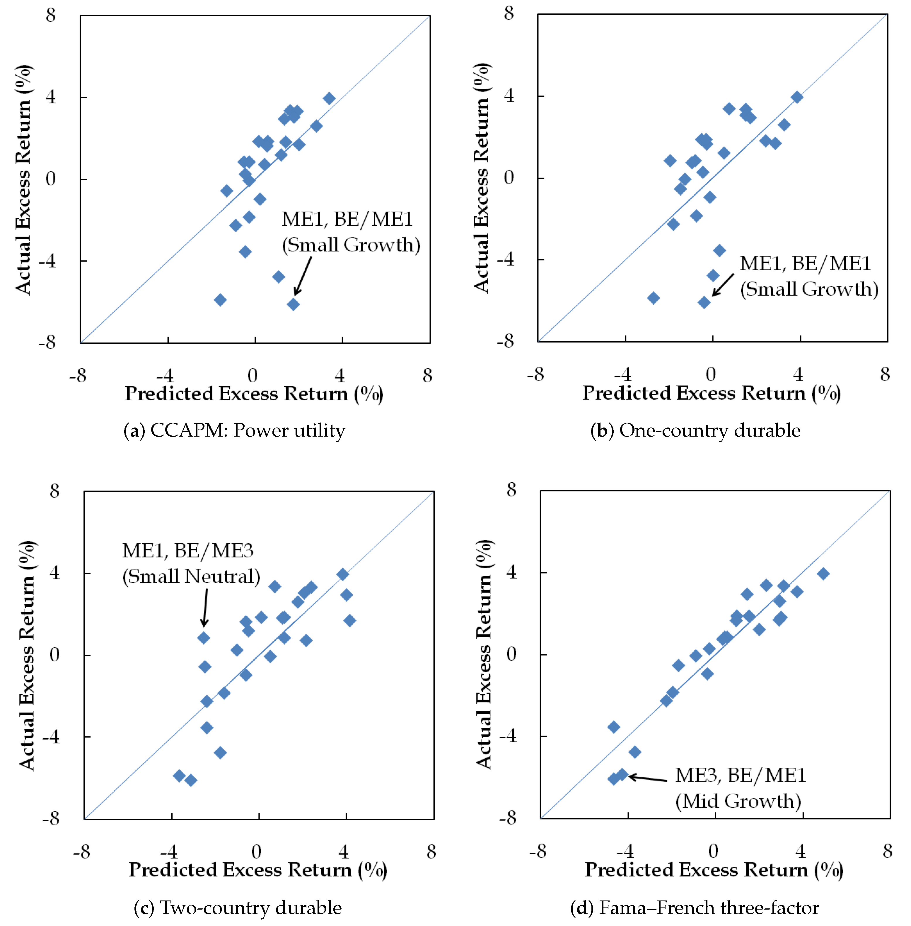
4.2.1. Estimation with 25 Fama–French Portfolios

Table 3. Estimation Results with 25 Fama–French Portfolios.

Factors	One-Country				Two-Country			CAPM	FF
	Power	EZ-ND	EZ-D		Power	EZ-ND	EZ-D
$C^{KR}$	106.804	125.375	145.411		129.554	98.903	19.493
	(5.082)	(6.816)	(8.592)		(6.567)	(8.337)	(6.243)
$D^{KR}$			−81.879				−23.068
			(8.568)				(10.909)
$R_w^{KR}$		−1.255	−0.745			18.980	0.617
		(1.117)	(1.210)			(1.888)	(2.203)
$C^{US}$					−70.982	286.791	−17.295
					(22.096)	(28.719)	(46.552)
$D^{US}$							408.203
							(53.161)
$R_w^{US}$						−53.160	−13.366
						(3.856)	(3.803)
$EXR$					0.000	0.051	0.276
					(1.155)	(1.765)	(1.868)
$Market$								0.117	2.731
								(0.163)	(0.195)
$SMB$									4.946
									(0.267)
$HML$									16.049
									(0.405)
$MAE(\%)$	1.647	1.745	1.829		1.755	1.572	1.405	2.279	0.778
$R^2$	0.242	0.273	0.345		0.269	0.450	0.633	−0.005	0.899
J-$test$	1.978	1.967	1.943		1.945	1.968	1.875	1.969	1.981
	(1.000)	(1.000)	(1.000)		(1.000)	(1.000)	(1.000)	(1.000)	(1.000)
(Wald Test)		$H_0$: $b_4=b_5=b_6=b_7=0$ in the two-country durable consumption model
			${\chi }^2=68.320(p=0.000)$

This table presents the GMM estimation results from the one- and two-country models, the CAPM, and the Fama–French three-factor model. Power is the linear factor model for a power utility. EZ-ND is the linear factor model with Epstein–Zin preferences for non-durable goods consumption. EZ-D is the linear factor model with Epstein–Zin preferences for durable goods consumption. FF is the Fama–French three-factor model. We report the estimated factor prices in each row. $C^i$, $D^i$, and $R_w^i$ represent non-durable consumption, durable consumption, and the return on wealth in country i, respectively. $EXR$ is the real exchange rate adjustment term for U.S. households. Factors related to Korean households have the superscript $KR$ and those related to U.S. households have the superscript $US$. $Market$ is the excess return for the market portfolio (KOSPI and KOSDAQ) in Korea. $SMB$ is the difference in the average returns between small and big stock portfolios. $HML$ is the difference in the average returns between high and low book-to-market equity stock portfolios. We present the mean absolute pricing errors ($MAE,\%$) and $R^2$s from the first-stage estimation. The numbers in parentheses below the coefficient estimates are Newey—West HAC standard errors. The p-values are in parentheses below the J-test values. The last row shows the Wald test of the joint hypothesis $H_0$: $b_4=b_5=b_6=b_7=0$ in the two-country durable consumption model. The p-values are in parentheses.

presents the GMM estimates of factor risk prices for the one-country and two-country models, the Fama–French three-factor model, and the CAPM. In the one- and two-country models, we use $Power$, $EZ$-$ND$, and $EZ$-D to represent the power utility, the Epstein–Zin non-durable consumption model, and the Epstein–Zin durable consumption model, respectively. In addition to the coefficient estimates, we report the mean absolute pricing errors (MAEs) and $R^2$s from the first-stage estimation. Here, we define $R^2$ as one minus the ratio of the variance of pricing errors to the variance of average portfolio returns, following Campbell and Vuolteenaho (2004).

The estimation results show that the one-country consumption-based models have lower $R^2$s or larger mean absolute pricing errors than their two-country counterparts.

The two-country models showed improvement over their one-country counterparts, except for the power utility CCAPM. In particular, our two-country durable consumption model yielded promising results. The mean absolute pricing error declined to 1.405% from 1.829% compared to its one-country counterpart and the $R^2$ almost doubled. Moreover, the Wald test strongly rejects the null hypothesis that the risk prices of the U.S. factors are all zeros, indicating that the foreign factors, which capture consumption heterogeneity, are important elements in pricing Korean stocks. In addition, compared with the two-country non-durable consumption model (EZ-ND), we found that the $R^2$ substantially increased from 0.450 to 0.633 by adding one variable, the durable consumption growth, as the durable consumption factor in the U.S. showed statistical significance at the 1% level.

Table 3 shows that the CAPM cannot adequately explain the average excess returns of the test assets. The failure of the CAPM for U.S. data is well-documented in the literature (Fama and French 1992, 1993; Yogo 2006). We found similar results for the Korean data. The risk price of the market portfolio is statistically insignificant and the mean absolute pricing error from the CAPM is sizable (2.279%). Moreover, the negative $R^2$ (−0.005) indicates a poor fit of the model, implying that it has less explanatory power than a model using only a constant that is equal to the cross-sectional average of the mean excess return.

The Fama–French three-factor model performs well in explaining the average excess return of the Fama–French portfolios. The model has a mean absolute pricing error of as low as $0.778\%$ and a large $R^2$ value of 0.899. These results are interesting. In fact, the Korean data exhibits the opposite pattern to the U.S. data in the spread between small- and large-cap stock portfolio returns ($SMB$)12. Despite this, our results suggest that the Fama–French three-factor model had considerable explanatory power for Korean data as well as U.S. data.

The J-statistics and p-values for the overidentifying restriction tests indicate that none of the models are rejected in the specification tests. However, despite the large pricing error and negative $R^2$, even the CAPM cannot be rejected by the test. This non-rejection may be due to the large variance of the pricing errors, which makes the J-statistic insignificant, rather than the model being a good fit. Therefore, in this case, the J-test may not provide informative results for evaluating the overall fit of the models. Similar findings were reported in other model specifications or comparison tests by Hodrick and Zhang (2001), Kan et al. (2013), and many others.

Figure 2a–d plot the predicted and actual excess returns for the 25 Fama–French portfolios in the selected models. Consistent with the GMM estimation results, the Fama–French three-factor model exhibits the smallest pricing error, as its predicted returns are aligned well with the 45-degree line. The pricing error of the two-country durable consumption model is smaller than those of other consumption-based models.

In Appendix A,

Table A1. Estimation with 25 Fama-French and 8 industry portfolios.

Factors	One-Country			Two-Country			CAPM	FF
	Power	EZ-ND	EZ-D	Power	EZ-ND	EZ-D
$C^{KR}$	90.067	90.612	119.073	87.680	79.302	67.962
	(2.697)	(2.714)	(3.765)	(2.792)	(3.995)	(5.556)
$D^{KR}$			−95.778			−26.357
			(5.038)			(7.313)
$R_w^{KR}$		−0.015	0.311		15.017	0.804
		(0.764)	(0.850)		(0.890)	(1.461)
$C^{US}$				9.843	318.164	−129.786
				(14.723)	(19.628)	(27.506)
$D^{US}$						280.533
						(16.725)
$R_w^{US}$					−45.683	−7.396
					(1.626)	(2.560)
$EXR$				0.000	0.000	0.064
				(0.596)	(1.059)	(1.052)
$Market$							0.307	2.631
							(0.154)	(0.139)
$SMB$								3.744
								(0.185)
$HML$								13.456
								(0.230)
$MAE(\%)$	1.693	1.699	1.687	1.669	1.415	1.334	2.074	1.044
$R^2$	0.176	0.176	0.291	0.176	0.452	0.571	−0.018	0.706
J-$test$	2.000	1.997	1.970	2.000	1.991	1.958	2.000	2.002
	(1.000)	(1.000)	(1.000)	(1.000)	(1.000)	(1.000)	(1.000)	(1.000)
(Wald Test)		$H_0$: $b_4=b_5=b_6=b_7=0$ in the two-country durable consumption model
			${\chi }^2=621.799(p=0.000)$

This table presents the GMM estimation results from our one- and two-country models, the CAPM, and the Fama–French three-factor model. Power is the linear factor model for a power utility. EZ-ND is the linear factor model with Epstein–Zin preferences for non-durable goods consumption. EZ-D is the linear factor model with Epstein–Zin preferences for durable goods consumption. FF is the Fama–French three-factor model. We report the estimated factor prices in each row. $C^i$, $D^i$, and $R_w^i$ represent non-durable consumption, durable consumption, and the return on wealth in country i, respectively. $EXR$ is the real exchange rate adjustment term for U.S. households. The superscripts $KR$ and $US$ denote factors from Korean and U.S. households, respectively. $Market$ represents the excess return for the market portfolio (KOSPI and KOSDAQ) in Korea. $SMB$ is the difference in the average returns between small and big stock portfolios. $HML$ is the difference in average returns between high and low book-to-market equity stock portfolios. We present the mean absolute pricing error ($MAE,\%$) and the $R^2$ from the first-stage estimation. The numbers in parentheses below the coefficient estimates are Newey–West HAC standard errors. The p-values for the J-test are reported in parentheses below the J-test values. The last row shows the Wald test of the joint hypothesis ($H_0$) in the two-country durable consumption model. The p-values are in parentheses.

shows the estimation results from the six above-mentioned models with the additional test assets of industry portfolios.13 The previous results remain largely unchanged. However, the explanatory power of the Fama–French three-factor model substantially deteriorates, more than that of the two-country durable consumption model. The $R^2$ for our model exhibits only a small decrease (from 0.633 to 0.571), whereas the Fama–French three-factor model exhibited a large decrease of about 0.2 (from 0.899 to 0.706). The actual and predicted excess returns are plotted in Figure A114 This figure indicates that the Fama–French three-factor model tends to have a higher degree of deviation of the predicted returns from actual returns, particularly for the IT industry profile.

4.2.2. Estimation Results with Selected Portfolios

In this section, we estimate the models using subgroups of test assets since unknown anomalies in some portfolios might not be captured by our model. For example, in Table 1, we can see that the average quarterly return for the BE/ME 1 group is $-3.3\%$, which is very low given that the aggregate market return is $2.1\%$, on average, over the sample period. This may imply that our model has only a limited ability to explain the return of portfolios with a relatively low BE/ME.

To further investigate whether the performance of our model depends on the characteristics of the test assets, we re-estimated the three models—the one-country durable consumption model, the two-country durable consumption model, and the Fama–French three-factor model—with selected subsets of portfolios. We employ the BE/ME2–BE/ME5 (20 portfolios) or BE/ME3–BE/ME5 (15 portfolios) groups in the subsequent analyses.

Table 4. Estimation using selected portfolios.

Factors	Panel A: BE/ME2–BE/ME5			Panel B: BE/ME3–BE/ME5
	EZ-D	EZ-D	FF	EZ-D	EZ-D	FF
	One-Country	Two-Country		One-Country	Two-Country
$C^{KR}$	116.062	74.203		93.718	49.942
	(8.127)	(10.180)		(7.871)	(9.963)
$D^{KR}$	39.499	58.473		50.975	78.394
	(7.894)	(15.853)		(13.321)	(17.205)
$R_w^{KR}$	0.9068	0.825		1.814	0.920
	(1.147)	(2.198)		(1.228)	(3.872)
$C^{US}$		9.986			209.734
		(30.907)			(47.478)
$D^{US}$		140.539			113.840
		(24.157)			(35.942)
$R_w^{US}$		−4.435			−9.256
		(4.186)			(6.410)
$EXR$		0.314			0.729
		(2.178)			(3.259)
$Market$			2.439			2.335
			(0.203)			(0.257)
$SMB$			4.513			4.362
			(0.304)			(0.436)
$HML$			13.567			12.431
			(0.417)			(0.555)
$MAE$	0.819	0.753	0.556	0.529	0.473	0.526
$R^2$	0.694	0.747	0.845	0.696	0.779	0.714
J-$test$	1.949	1.846	1.971	1.843	1.567	1.827
	(1.000)	(1.000)	(1.000)	(1.000)	(0.992)	(1.000)
(Wald Test)			$H_0:b_4=b_5=b_6=b_7=0$
	BE/ME2–BE/ME5			BE/ME3–BE/ME5
	${\chi }^2=103.69(p=0.000)$			${\chi }^2=139.32(p=0.000)$

This table presents the GMM estimation results from our one- and two-country durable consumption models and the Fama–French three-factor model using the selected portfolios. EZ-D is the linear factor model with Epstein–Zin preferences for durable goods consumption. FF is the Fama–French three-factor model. We report the estimated factor prices in each row. The first three estimates are from portfolios that include the BE/ME2–BE/ME5 groups. The next three size portfolios include the BE/ME2–BE/ME5 groups. $C^i$, $D^i$, and $R_w^i$ represent the non-durable consumption, durable consumption, and return on wealth in country i, respectively. $EXR$ is the real exchange rate adjustment term for U.S. households. Factors related to Korean households have the superscript $KR$ and those related to U.S. households have the superscript $US$. $Market$ is the excess return for the market portfolio (KOSPI and KOSDAQ) in Korea. $SMB$ is the difference in the average returns between small and big stock portfolios. $HML$ is the difference in the average returns between high and low book-to-market equity stock portfolios. We show the mean absolute pricing error ($MAE,\%$) and the $R^2$ from the first-stage estimation. The numbers in parentheses below the coefficient estimates are the Newey–West HAC standard errors. The p-values for the J-test are shown below the J-test values in parentheses. The last row shows the Wald test of the joint hypothesis $H_0$:$b_4=b_5=b_6=b_7=0$ for the two-country durable consumption model. The p-values are in parentheses.

summarizes the estimation using the selected portfolios. Panel A shows estimates from the portfolios in the BE/ME2–BE/ME5 groups using the three models. It can be seen that the one-country durable consumption model has significant positive risk prices for non-durable and durable consumption. The risk price for wealth is positive but is not significantly different from zero. The mean absolute error and the $R^2$ for the one-country model were 0.819% and 0.694, respectively.

The two-country durable consumption model performs better in explaining the average excess returns of these portfolios than the one-country durable consumption model. The model delivers a low mean absolute pricing error of 0.753% and the Wald test strongly rejects the null hypothesis that the U.S. factors are jointly unrelated in explaining the expected return of the Korean assets. We can also see that the coefficient for U.S. durable consumption is significant at the 1% level, as the coefficients are also significant for non-durable and durable consumption growth in Korea.

The Fama–French three-factor model still performs the best for the BE/ME2–BE/ME5 groups, yielding the smallest mean absolute pricing error (0.556%) and the highest $R^2$ (0.845) among the considered models. However, as the performance of the two-country durable model improved, the difference in explanatory power between the two models became small.

Panel B presents the estimates for the BE/ME3–BE/ME5 groups. As in the BE/ME2–BE/ME5 groups, the one-country durable consumption model has significant risk prices for both non-durable and durable consumption. The mean absolute error and $R^2$ for the one-country model are 0.529% and 0.696, respectively, similar to those of the 20-portfolio BE/ME2–BE/ME5 groups.

The two-country durable consumption model can explain the average excess returns of these 15 portfolios reasonably well. The model has a low mean absolute average pricing error of 0.473% and quite a large $R^2$ value (0.779). The coefficients have the same signs as the 20 portfolios, and those of non-durable and durable consumption growth in both countries are significant at the 1% level.

Notably, the risk price is significant not only for Korean durable consumption growth but also for U.S. durable consumption growth for all the samples above. Yogo (2006) found that durable consumption growth had a significant risk price15 in explaining domestic stock returns in the U.S. Our empirical finding implies that his results can be extended to pricing Korean assets of which U.S. investors hold a considerable share.

For the BE/ME3–BE/ME5 groups, the Fama–French three-factor model has larger pricing errors than our model. The three-factor model delivered an MAE of 0.526%, which is larger than the 0.473% of our model. The $R^2$ dropped from 0.845 to 0.714 when we excluded BE/ME2 from the test assets, indicating that the better performance of the three-factor model compared to our model could be attributed to its explanatory power for portfolios with relatively low BE/ME ratios.

Figure 3 shows the pricing errors from the two-country durable consumption and the Fama–French three-factor models for the two classes of selected portfolios. Figure 3a,b show the pricing errors from the two models for the BE/ME2–BE/ME5 portfolios and Figure 3c,d plot the pricing errors for the BE/ME3–BE/ME5 portfolios. In particular, Figure 3c,d illustrate that our model had smaller pricing errors than the Fama–French three-factor model for the test assets. As we reduced the number of portfolios, some estimates showed larger changes, for example, the risk price of U.S. non-durable consumption jumped from 9.986 to 209.734. Hence, the predicted returns from the two-country durable consumption model moved closer to the 45-degree line, whereas most of the predicted returns from the Fama–French three-factor model remained unchanged.

In an unreported analysis, we also estimated the above three models using size-based portfolios. We used 20 portfolios in the ME2–ME5 groups and 15 portfolios in the ME3–ME5 groups, including all the BE/ME portfolios in each corresponding size group. The significance of the U.S. factors in our two-country durable consumption model was maintained in the Wald tests for these subsamples, although the Fama–French model performed better in terms of pricing errors.

To summarize, the overall performance of the three-factor model was significantly better than that of the two-country durable consumption model, but the estimation results on the subgroups show that our model has some merits in explaining the returns of value stocks. So far, we have compared the performance of the models without any formal statistical tests. In Section 4.2.3, we further investigate whether the performance of the two models was statistically different based on tests proposed by Kan et al. (2013).

4.2.3. Equality Tests of Cross-Sectional $R^2$s

This section compares the performance of our model and the Fama–French three-factor model using a formal statistical test. We used the Kan et al. (2013) test for non-nested models,16 hereafter referred to as the KRS test, to test the statistical significance of the difference in cross-sectional $R^2$ between the two models.17 One of the key advantages of the KRS test is that we can remain agnostic about the “true” model, as originally advocated by Hansen and Jagannathan (1997). It is worth noting that all models have the potential to be misspecified since they are only imperfect representations of reality. Hence, the tests provided by Kan et al. (2013) are robust to potential model misspecification. Thus, even if neither the two-country durable nor the Fama–French three-factor model was true, it would be possible to evaluate the relative performance of the two models in terms of the model fit. Another advantage of the KRS test is that it is applicable to not only OLS $R^2$s but also GLS $R^2$s.18 As documented by Kan et al. (2013), in an analysis with excess returns, testing the difference between GLS $R^2$s is equivalent to testing the equality of Hansen–Jagannathan (HJ) distances.19 Thus, the difference in the GLS $R^{2}s$ can be interpreted as the difference in the maximum pricing error.

Table 5. Equality tests of cross-sectional $R^2$s.

	25 Fama–French	BE/ME2	BE/ME3	25 Fama–French
		–BE/ME5	–BE/ME5	+8 Industries
Panel A: OLS
${\rho }_{2cd}^2$	0.800	0.872	0.938	0.738
$s.e$	(0.035)	(0.062)	(0.030)	(0.096)
${\rho }_{ff3}^2$	0.900	0.901	0.910	0.718
$s.e$	(0.044)	(0.064)	(0.070)	(0.058)
${\rho }_{2cd}^2-{\rho }_{ff3}^2$	−0.100	−0.029	0.028	0.020
p-value	[0.008]	[0.522]	[0.591]	[0.829]
Panel B: GLS
${\rho }_{2cd}^2$	0.208	0.372	0.483	0.269
$s.e$	(0.068)	(0.133)	(0.093)	(0.080)
${\rho }_{ff3}^2$	0.571	0.508	0.448	0.368
$s.e$	(0.157)	(0.154)	(0.147)	(0.062)
${\rho }_{2cd}^2-{\rho }_{ff3}^2$	−0.364	−0.136	0.035	−0.098
p-value	[0.187]	[0.261]	[0.878]	[0.187]

This table presents the results of the equality tests of the cross-sectional $R^2$s for the two-country durable consumption model and the Fama–French three-factor model. ${\rho }_i^2$ is the cross-sectional $R^2$ of model i. The subscripts $2cd$ and $ff3$ denote the two-country durable consumption model ($2cd$) and the Fama–French three-factor model, respectively. The numbers in parentheses are the standard errors. ${\rho }_{2cd}^2-{\rho }_{ff3}^2$ is the difference between the $R^2$s of the two models. The numbers in brackets are the p-values for the test of $H_0:0<{\rho }_{2cd}^2={\rho }_{ff3}^2<1$. Following the methodology of Kan et al. (2013), we computed the p-values, assuming potential model misspecification. Panels A and B show the results for the OLS and GLS estimations, respectively.

summarizes the statistics for the KRS tests. In the table, $R^2$s are denoted by ${\rho }^2$s to distinguish them from the $R^2$s used in the previous sections. Panels A and B, respectively, show the OLS and GLS $R^2$s for four sets of test assets: 25 Fama–French portfolios, 20 portfolios of BE/ME2–BE/ME5 groups, 15 portfolios of BE/ME3–BE/ME5 groups, and 25 Fama–French + 8 industry portfolios. The performance of both models, as shown in Panel A, was quite impressive. The OLS $R^2$s are relatively high, being close to 0.9 for most of the subsample analyses. The differences in the OLS $R^2$s of the two models are small in magnitude and they are not statistically different from zero in all but one case in the first column. For the sample of the 25 Fama–French portfolios, the Fama–French three-factor model has a significantly higher $R^2$ at the 1% level. However, for the other three samples, the differences in the $R^2$s are not statistically significant. The p-values of the KRS tests for the BE/ME2–BE/ME5 groups, BE/ME3–BE/ME5 groups, and 25 Fama-French + 8 industries are greater than 50%, whereas the $R^2$s of our model are slightly higher than those of the Fama–French three-factor model for the BE/ME3–BE/ME5 groups and 25 Fama-French + 8 industry portfolios.

Panel B indicates that the GLS $R^2$ (equivalently, the HJ distances) are not statistically different between the two models across all choices of test assets. In the first column, the GLS $R^2$ of the Fama–French three-factor model (0.571) is much larger than that of the two-country durable model (0.208). Nonetheless, the results of the KRS test suggest that the Fama–French three-factor model does not outperform the two-country durable model when sampling variation is taken into account. As its GLS standard error (0.157) for all portfolios is almost quadrupled, compared to its OLS standard error (0.044), the KRS test fails to reject the null hypothesis that their HJ distances were equal. The test yielded similar results for the other choices of test assets.

In summary, from a statistical perspective, our model’s performance is comparable to that of the Fama–French three-factor model in most cases. We observed that the differences between the standard OLS $R^2$s and the HJ distances were statistically insignificant, except for only one case, the OLS $R^2$ for 25 portfolios. Thus, by judging the magnitudes of the $R^2$s and using inferences from the statistical tests, we did not find strong evidence to support the use of the Fama–French three-factor model over our two-country durable consumption model.

5. Conclusions

For U.S. data, the empirical success of the Fama–French three-factor model is well-known. We found that the three-factor model could adequately explain the cross-section of Korean stocks. However, as Fama (1991) and Fama and French (1992) suggested, the two factors HML and SMB are not easily interpreted within an economic framework. For this reason, many versions of equilibrium asset pricing models have been proposed and their empirical performance has been investigated. In this area of research, Yogo (2006) has made important progress in addressing the failures of standard consumption-based models that rely only on aggregate or non-durable consumption. He found that durable consumption played a significant role in pricing assets through the elasticity of substitution between durable and non-durable consumption. Employing the durable consumption model of Yogo (2006), we incorporated the foreign SDF into the model, assuming market incompleteness. Our two-country durable consumption model produced promising results, suggesting that the U.S. SDF helped to capture the cross-sectional variations in Korean stock returns. The foreign factors in our model are jointly significant and this model even yielded a lower average pricing error for high book-to-market equity (BE/ME3–BE/ME5) portfolios than the Fama–French three-factor model. In particular, the compensation of Korean stocks is robust for the durable consumption risk in the U.S. across all the samples we considered. Moreover, from the KRS tests, we found that the explanatory power of the model was comparable to that of the Fama–French three-factor model in most cases.

To the best of our knowledge, this paper is the first to incorporate foreign pricing factors into the SDF to investigate the influence of foreign investors on domestic stock returns. Our empirical findings suggest that cross-country consumption heterogeneity is essential for pricing assets in financial markets where foreign investors hold a large share. Given this implication, good candidates for further research would be countries such as the U.K., France, and the Netherlands, since the share of holdings by non-residents is also large in these countries.

References

1. Bae, Kee-Hong, Kalok Chan, and Angela Ng. 2004. Investibility and Return Volatility. Journal of Financial Economics 71: 239–63. [Google Scholar] [CrossRef]
2. Bansal, Ravi, Thomas D. Tallarini, and Amir Yaron. 2008. The Return to Wealth, Asset Pricing and the Intertemporal Elasticity of Substitution. Society for Economic Dynamics 2008 Meeting Papers 918. Available online: https://econpapers.repec.org/paper/redsed008/918.htm (accessed on 20 January 2020).
3. Bekaert, Geert, Campbell R. Harvey, and Christian Lundblad. 2005. Does financial liberalization spur growth? Journal of Finance 77: 3–55. [Google Scholar] [CrossRef]
4. Brennan, Michael J., and H. Henry Cao. 1997. International Portfolio Investment Flows. Journal of Finance 52: 1851–80. [Google Scholar] [CrossRef]
5. Brennan, Michael J., H. Henry Cao, Norman Strong, and Xinzhong Xu. 2005. The Dynamics of International Equity Market Expectations. Journal of Financial Economics 77: 257–88. [Google Scholar] [CrossRef]
6. Campbell, John Y. 1996. Understanding Risk and Return. Journal of Political Economy 104: 298–345. [Google Scholar] [CrossRef]
7. Campbell, John Y., and Tuomo Vuolteenaho. 2004. Bad Beta, Good Beta. American Economic Review 94: 1249–75. [Google Scholar] [CrossRef]
8. Chan, Kalok, Albert J. Menkveld, and Zhishu Yang. 2008. Information Asymmetry and Asset Prices: Evidence from the China Foreign Share Discount. Journal of Finance 63: 159–96. [Google Scholar] [CrossRef]
9. Chari, Anusha, and Peter B. Henry. 2004. Risk Sharing and Asset Prices: Evidence from a Natural Experiment. Journal of Finance 59: 1295–324. [Google Scholar] [CrossRef]
10. Choe, Hyuk, Bong-Chan Kho, and Rene M. Stulz. 1999. Do Foreign Investors Destabilize Stock Markets? The Korean Experience in 1997. Journal of Financial Economics 54: 227–64. [Google Scholar] [CrossRef]
11. Colacito, Riccardo, and Mariano M. Croce. 2011. Risks for the Long Run and the Real Exchange Rate. Journal of Political Economy 119: 153–81. [Google Scholar] [CrossRef]
12. Constantinides, George M., and Darrell Duffie. 1996. Asset Pricing with Heterogeneous Consumers. Journal of Political Economy 104: 219–40. [Google Scholar] [CrossRef]
13. Croce, Mariano M. 2014. Long-run productivity risk: A new hope for production-based asset pricing? Journal of Monetary Economics 66: 13–31. [Google Scholar] [CrossRef]
14. Darrat, Ali F., Bin Li, and Jung Chul Park. 2011. Consumption-based CAPM models: International evidence. Journal of Banking & Finance 35: 579–601. [Google Scholar]
15. Eyster, Erik, Matthew Rabin, and Dimitri Vayanos. 2019. Financial Markets Where Traders Neglect the Informational Content of Prices. Journal of Finance 74: 371–99. [Google Scholar] [CrossRef]
16. Fama, Eugene F. 1991. Efficient Capital Markets: II. Journal of Finance 46: 1575–617. [Google Scholar] [CrossRef]
17. Fama, Eugene F., and Kenneth R. French. 1992. The Cross-Section of Expected Stock Returns. Journal of Finance 47: 427–65. [Google Scholar] [CrossRef]
18. Fama, Eugene F., and Kenneth R. French. 1993. Common Risk Factors in the Returns on Stocks and Bonds. Journal of Financial Economics 33: 3–56. [Google Scholar] [CrossRef]
19. Fogli, Alessandra, and Fabrizio Perri. 2015. Macroeconomic Volatility and External Imbalances. Journal of Monetary Economics 69: 1–15. [Google Scholar] [CrossRef]
20. Hansen, Lars Peter, and Ravi Jagannathan. 1997. Assessing specification errors in stochastic discount factor models. The Journal of Finance 52: 557–90. [Google Scholar] [CrossRef]
21. Hodrick, Robert J., and Xiaoyan Zhang. 2001. Evaluating the Specification Errors of Asset Pricing Models. Journal of Financial Economics 62: 327–76. [Google Scholar] [CrossRef]
22. Jeong, Daehee, Hwagyun Kim, and Joon Y. Park. 2015. Does Ambiguity Matter? Estimating Asset Pricing Models with a Multiple-Priors Recursive Utility. Journal of Financial Economics 115: 361–82. [Google Scholar] [CrossRef]
23. Kaltenbrunner, Georg, and Lars Lochstoer. 2010. Long-run risk through consumption smoothing. Review of Financial Studies 23: 3141–89. [Google Scholar] [CrossRef]
24. Kan, Raymond, Cesare Robotti, and Jay Shaken. 2013. Pricing model performance and the two-Pass cross-sectional regression methodology. Journal of Finance 68: 2617–49. [Google Scholar] [CrossRef]
25. Li, Yuming, and Maosen Zhong. 2005. Consumption Habit and International Stock Returns. Journal of Banking & Finance 29: 579–601. [Google Scholar]
26. Lustig, Hanno, and Stijn Van Nieuwerburgh. 2008. The Returns on Human Capital: Good News on Wall Street Is Bad News on Main Street. The Review of Financial Studies 21: 2097–137. [Google Scholar] [CrossRef]
27. Sarkissian, Sergei. 2003. Incomplete Consumption Risk Sharing and Currency Risk Premiums. Review of Financial Studies 16: 983–1005. [Google Scholar] [CrossRef]
28. Stiglitz, Joseph E. 2004. Capital Market Liberalization, Globalization, and the IMF. Oxford Review of Economic Policy 20: 57–71. [Google Scholar] [CrossRef]
29. Umutlu, Mehmet, Levent Akdeniz, and Aslihan Altay-Salih. 2010. The Degree of Financial Liberalization and Aggregated Stock-Return Volatility in Emerging Markets. Journal of Banking & Finance 34: 509–21. [Google Scholar]
30. Yogo, Motohiro. 2006. A Consumption-Based Explanation of Expected Stock Returns. Journal of Finance 61: 539–80. [Google Scholar] [CrossRef]
31. Yun, Sang Yong, Bonil Ku, Young Ho Eom, and Jaehoon Hahn. 2009. The Cross-Section of Stock Returns in Korea: An Empirical Investigation. Asian Review of Financial Research 22: 1–44. [Google Scholar]
Figure 1. Shares held by foreign investors in Korea. (a) Shares held by foreign investors in the Korean stock markets (KOSPI and KOSDAQ). (b) Composition of foreign investors by nationality. The data are from the Financial Supervisory Service.
Ijfs 11 00062 g001
Figure 2. Actual and predicted excess returns for Fama–French portfolios. The figures plot the actual and predicted excess returns for the 25 Fama–French portfolios. The portfolios are sorted by size and book-to-market equity. Predicted excess returns are from (a) the CCAPM for the power utility, (b) the one-country model for durable consumption, (c) the two-country model for durable consumption, and (d) the Fama–French three-factor model. The returns are shown as quarterly values.
Ijfs 11 00062 g002
Figure 3. Actual and predicted excess returns for selected portfolios. This figure plots the actual and predicted excess returns for the 15 selected portfolios. The portfolios are sorted by size and book-to-market equity. The predicted excess returns are from (a) the two-country durable consumption model with BE/ME2–BE/ME5 portfolios, (b) the Fama–French three-factor model with BE/ME2–BE/ME5 portfolios, (c) the two-country durable consumption model with BE/ME3–BE/ME5 portfolios, and (d) the Fama–French three-factor model with BE/ME3–BE/ME5 portfolios. The returns are shown as quarterly values.
Ijfs 11 00062 g003