Anomalies and Investor Sentiment: International Evidence and the Impact of Size Factor

Abstract

We examine whether investor sentiment can explain anomalies such as size and book-to-market in the US stock market. Differently from the literature, we test combination portfolios (portfolios formed on more than one factor such as size, book-to-market ratio, etc.) of developed markets for the same purpose. We find that sentiment is related to some anomalies in Europe, Japan, North America and global portfolios; hence, the sentiment and anomaly relationship may be universal. In addition, when size factor is controlled, the explanatory power of sentiment in anomaly returns changes.

1. Introduction

Although the efficient markets hypothesis (EMH) claims that there is no free lunch in the sense that asset prices reflect all available information, a vast body of research bolsters the opposite opinion. Several strategies, e.g., size and value, have been found to result in returns that are higher than what is anticipated by Fama–French’s three-factor model (Fama and French 1993). For instance, size strategy (or size anomaly) contends that going long with small sized stocks and (simultaneously) short with large sized stocks produces a higher return than that anticipated by common asset pricing models, i.e., it generates a positive alpha (Banz 1981). Fama and French (1992) documented that stocks with higher book-to-market ratios have a higher risk-adjusted return compared to stocks with lower ratios.

Anomalies are not limited to size and book-to-market ratio. Momentum (Jegadeesh and Titman 1993), asset growth (Cooper et al. 2008), January (Keim 1983; Reinganum 1983), and contrarian (De Bondt and Thaler 1985) effects are among the well-known market anomalies. Lu et al. (2017) indicated that several anomalies exist, not only in the US but also in Canada, France, Germany, Japan and the UK.

Researchers have long been attempting to explore the reasons behind anomalies. Among them, Stambaugh et al. (2012) advocated that anomalies can be explained by investor sentiment. Additionally, Altanlar et al. (2019); Zaremba (2016); Jacobs (2015) and Ali and Gurun (2009) argue that investor sentiment plays a key role in anomaly returns.

Motivated by these arguments, we investigated anomalies for various countries and with different portfolio sets. We first checked whether there were anomalies in the US stock market. Then, using predictive analysis, we showed that investor sentiment explains anomalies such as size and investments in the US stock market. We examined regions other than the US by using portfolio returns based upon binary combinations of anomalies. Our findings indicate that when size impact is removed, the power of sentiment to explain anomaly returns changes. The findings and the method (using combination portfolios) are supported by the robustness checks.

This study contributes to the literature in various ways. To explain anomalies, we followed Stambaugh et al. (2012), yet included more anomalies than they did. Moreover, we used the Fama–French five-factor model (Fama and French 2015) while they used the Fama–French three-factor model. We tested fifteen different factors and examined long–short strategies in the US stock market. Furthermore, we based our strategy on portfolios containing combinations of different anomalies and composed of European, Japanese, North American and global assets, assuming that each market can exhibit different anomalies. We examined the explanatory power of sentiment in anomaly strategies by controlling the size factor. For instance, we examined the book-to-market anomaly on stocks with small market capitalization and big market capitalization separately. Hence, our research opens up new ground for anomaly research in terms of considering stock characteristics and proposes a new practice (using combination portfolios).

This paper is organized as follows. Section 2 reviews the literature related to anomalies and investor sentiment. Section 3 summarizes the data and models. Section 4 lists the empirical results and displays robustness checks. Section 5 concludes this study.

2. Literature Review

The anomaly literature has gained traction after Banz (1981) argued that small cap stocks have higher risk-adjusted returns than large cap stocks. Thereafter, the phenomenon was called the size effect. Though widely used in trading strategies afterwards, Schwert (2003) stated that this effect disappeared in the subsequent years. One decade later, Fama and French (1992) detected a correlation between book-to-market ratio and stock returns in the US stock market, known as the book-to-market anomaly. This idea has attracted keen interest among scholars and influenced countless studies through the years. Based on previous price dynamics, the momentum effect is another anomaly that cannot be explained by asset pricing models. According to this effect, stocks that recorded have previously a rise perform better in the upcoming months (Jegadeesh and Titman 1993). Yet, when the time horizon is extended, the results might not be the same. De Bondt and Thaler (1985) showed that stocks performing worse in the last three years beat other stocks in the following three years, referred to as the reversal (contrarian) effect. Keim (1983) and Reinganum (1983) found evidence of the January effect, which is when small stocks yield more in the month of January. More recently, Cooper et al. (2008) indicated that stocks with lower asset growth record higher risk-adjusted returns, a phenomenon called the asset growth anomaly. Sloan (1996) documented the accrual anomaly, which is the opposite predictive relationship between accounting accruals and stock returns.

Several studies show that anomalies exist not only in the US but also in many other countries. The book-to-market anomaly has also been validated for the Japanese stock market (Chan et al. 1991). In turn, Griffin et al. (2003) showed that the momentum effect is not particular to the US but exists in other countries as well. Lu et al. (2017) found many of the aforementioned anomalies in Europe, Canada, Japan and the UK. It is worth noting that while examining return data, dependence and nonlinearity may create issues. For instance, Ferreira and Dionísio (2014) indicated that Japanese and Canadian index data carry random walk whereas several other indices do not.

Obviously, the existence of these anomalies is a challenge for the efficient markets hypothesis. Many researchers seek answers for market anomalies. For instance, according to De Bondt and Thaler (1985), reversal occurs due to overreaction. Conversely, according to Jegadeesh and Titman (1993), the momentum effect exists because of underreaction. Nonetheless, the literature is far from reaching consensus on the causes of these anomalies. In the last decade, certain researchers have focused on the role of investor sentiment in explaining anomalies. For example, Lee et al. (2002) found that positive changes in sentiment lead to higher excess returns and not only in small stocks. Brown and Cliff (2005) indicate that sentiment affects asset valuations and that pricing models should include investor sentiment. Stambaugh et al. (2012) stated that investor sentiment can explain the excess return obtained by implementing strategies based upon anomalies. Altanlar et al. (2019) claimed that cognitive dissonance caused by sentiment and culture could be the reason for momentum and post-earnings-announcement drifts. Zaremba (2016) found that investor sentiment affects cross-country stock market anomalies. Jacobs (2015) tested one hundred anomaly strategies and concluded that sentiment has a role in explaining anomalies. Ali and Gurun (2009) related the accruals anomaly to investor sentiment. Stambaugh and Yuan (2017) suggested a new asset pricing model with two mispricing factors by using information from 11 anomalies in order to explain anomaly returns. Authors have argued that their model performs well, and that sentiment predicts these mispricing factors. On the other hand, Kim and Na (2018) did not find the same result regarding the relationship between anomaly and sentiment when they incorporated macroeconomic variables.

Anomaly trading has become more prominent following the publication of related academic papers and investor attention days. Calluzzo et al. (2019) indicated that anomaly-based trading occurs after an anomaly is announced in an academic paper, and that institutional investors play a key role in arbitrage trading and hence bolster market efficiency. In turn, Jiang et al. (2021) indicated that anomaly returns are higher right after high investor attention days. The authors also showed that large traders are more active following high attention days. Supporting Schwert (2003), Jacobs and Müller (2019) find that long–short returns of anomalies decrease after the publication of anomalies.

Several studies have examined the relationship between sentiment and anomalies for different countries. For example, Han and Shi (2022) found that investor sentiment is able to predict anomaly returns in China. Yang et al. (2017) showed that investor sentiment has a significant effect on stock returns in Korea, and that the impact is stronger on stocks with small size, high book-to-market ratio, high volatility and high excess return. Moreover, Bathia and Bredin (2013) indicated that the returns of value stocks in G7 countries are more prone to sentiment effect. These examples reveal that the relationship between sentiment and market anomalies needs to be investigated in more detail.

3. Data and Methodology

3.1. Data

Listed in

Table 1. Dataset.

Country/Region	Data Period	Nb of Months	Sentiment Indicators
US	January 1978–September 2015	453	Baker and Wurgler, U Michigan
Japan	March 2004–October 2018	176	Japanese CCI
Europe	July 1990–October 2018	340	ESI
North America	November 1990–September 2015	299	Baker and Wurgler, U Michigan
Global	November 1990–September 2015	299	Baker and Wurgler, U Michigan

Notes: Our dataset consists of five countries or regions (US, Japan, Europe, North America and global) and monthly portfolio return data and investor sentiment index data from 1978, 1990,2004 to 2015, and 2018, depending on the country or region.

, our dataset consists of monthly portfolio return data and investor sentiment index data for five countries or regions (US, Japan, Europe, North America and World) from 1978, 1990, 2004 to 2015, and 2018, depending on the country or region. Hence, the focus is to analyze major markets and regions over a long time period.

So far, several sentiment indicators have been developed and are commonly used by both academics and practitioners. Among them are the University of Michigan consumer sentiment index, which is a direct indicator1, and Baker and Wurgler (2006)’s sentiment index, which is an indirect indicator, both originally launched in the US. Japanese consumer confidence index (CCI)2 and the economic sentiment indicator (ESI3) of Europe4 are direct sentiment indicators.

Other than the US, Japan and Europe, we conducted the same analysis for North American and global portfolios by using the US sentiment indicators as a proxy because Baker et al. (2012) indicated that the correlation between sentiment indicators of the US and Canada is 0.60, and that the US sentiment indicator has the highest correlation with the authors’ global sentiment indicator.

Narayan and Sharma (2015) and Narayan et al. (2015) argued that financial models can be data-frequency-dependent. Hence, selecting the right frequency reveals crucial in hypothesis testing. In this study, we employed monthly frequency following the major papers in this field (e.g., Stambaugh et al. 2012; Jacobs 2015) that opt for monthly frequency, possibly due to the unavailability of the sentiment data at other frequencies. As is typical in the literature, our sentiment data (Baker and Wurgler as well as consumer confidence indices) were released on monthly basis.

Our examination of anomalies equally varied across countries and regions. For instance, we investigated fifteen different anomalies for the US while only five for Japan, Europe, North America and the globe. These are tabulated in

Table 2. Anomalies analyzed in this paper.

Anomaly	Reference	Strategy
Size	Banz (1981)	Decile 1–Decile 10
Book-to-market	Fama and French (1992)	Decile 10–Decile 1
Momentum	Jegadeesh and Titman (1993)	Decile 10–Decile 1
Operating profitability	Fama and French (2016); Chen et al. (2011)	Decile 10–Decile 1
Investments (asset growth)	Cooper et al. (2008)	Decile 1–Decile 10
Short-term reversal	Jegadeesh (1990)	Decile 1–Decile 10
Long-term reversal	De Bondt and Thaler (1987)	Decile 1–Decile 10
Accruals	Sloan (1996)	Decile 1–Decile 10
Cashflow/price	Hackel et al. (2000)	Decile 10–Decile 1
Dividend yield	Naranjo et al. (1998)	Decile 10–Decile 1
Earnings/price	Basu (1977, 1983)	Decile 10–Decile 1
Market beta	Frazzini and Pedersen (2014)	Decile 1–Decile 10
Net share issues	Loughran and Ritter (1995); Daniel and Titman (2006); Fama and French (2016)	Decile 1–Decile 10
Residual variance	Ang et al. (2006)	Decile 1–Decile 10
Variance	Ang et al. (2006)	Decile 1–Decile 10

Notes: The table shows fifteen different anomalies included in the analysis. We investigated all the anomalies for the US portfolio whereas only first five anomalies for Japan, Europe and global portfolios were investigated. Portfolios are separated into 10 groups based on these anomalies. For instance, for size anomaly, Decile 1 includes the stocks with the smallest and Decile 10 includes the stocks with the largest market cap. A strategy consists of taking a long position in one extreme portfolio and simultaneously a short position in the opposite extreme. As an example, “Decile 1–Decile 10” means buying Decile 1 portfolio and selling Decile 10 portfolio.

.

Before starting anomaly studies, stocks are divided into 10 deciles (groups) according to factors (anomalies) such as size, book-to-asset ratio and market beta. An anomaly strategy consists of taking a long position in stocks with an extreme decile and a short position in stocks with the opposite extreme decile (e.g., for size strategy, going long with the decile having the stocks with the lowest sizes, and going short with the decile having the stocks with the largest sizes). These strategies are listed in Table 2.

In anomaly studies, an anomaly strategy is simulated, and the return of this simulation is regressed using various independent variables (in our case, sentiment indicators), along with control variables (as in Stambaugh et al. (2012)). However, before this step, we checked whether anomalies existed (returns were regressed along with control variables, excluding sentiment).

To do so, we calculated “anomaly strategy” (also called “hedge strategy”) returns for the US. On the other hand, for other regions—as opposed to the current literature—we calculated portfolio returns based upon binary combinations of anomalies due to lack of return data for pure anomaly portfolios. For instance, we used six available portfolios composed of stocks sorted according to their size and book-to-market value (classified as “small” and “big” for size and “low”, “mid” and “high” for book-to-market value), as illustrated in

Table 3. Combination portfolios based on size and book-to-market values.

	Pf 1	Pf 2	Pf 3	Pf 4	Pf 5	Pf 6
Size	Small	Small	Small	Big	Big	Big
Book-to-market	Low	Mid	High	Low	Mid	High

Note: The table shows binary combinations of portfolios sorted for size and book-to-market ratio. For example, the first portfolio (Pf 1) consists of stocks with small size and low book-to-market ratio whereas the last portfolio (Pf 6) consists of stocks with big size and high book-to-market ratio. Portfolio data belong to the Kenneth French Data Library.

. Each portfolio is a binary combination of size and book-to-market ratio. In this example, the first portfolio consists of stocks with a small size and low book-to-market ratio whereas the last portfolio consists of stocks with a big size and high book-to-market ratio. All the data to calculate pure portfolio returns are obtained from Kenneth French’s data library.

In order to calculate the return of the low book-to-market strategy, we averaged the return of the portfolio consisting of stocks with a small size and low book-to-market ratio (Pf 1), and that of the portfolio consisting of stocks with a big size and low book-to-market ratio (Pf 4). We argue that this method provides the return of a pure low book-to-market strategy because the averaging process removes the impact of size (we preferred to use equally weighted portfolios instead of value-weighted portfolios for this analysis in order to eliminate the impact of market capitalization). Similarly, for a high book-to-market strategy, we averaged the returns of Pf 3 and Pf 6. Accordingly, the difference between high and low book-to-market strategy returns revealed the return of book-to-market anomaly (i.e., taking a long position in stocks with high book-to-market ratios and simultaneously taking a short position in stocks with low book-to-market ratios). Investment, operating profitability and momentum strategies were calculated analogously.

Aside from the pure anomaly portfolios, we found the outcome of these strategies when the size factor was fixed. In other words, we analyzed the book-to-market anomaly in two different cases; in one case, the size was “small” and in the other case, the size was “big”. Hence, we were able to measure the impact of size on other strategies.

In this second method (i.e., fixing size factor), the calculation of our dependent variable (i.e., anomaly strategy return, in which size factor was fixed) was straightforward. The third portfolio (Pf 3) minus the first portfolio (Pf 1) produced results for a book-to-market strategy when size was small, i.e., the strategy included stocks with small market capitalization. Accordingly, Pf 6 minus Pf 4 could be used to measure book-to-market anomaly when size was big. Investment, operating profitability and momentum strategies were examined analogously.

3.2. Models

On the empirical side, we primarily tested the existence of anomalies with reference to two alternative models extensively used in the literature. These were the Fama–French three-factor model (FF3F) and Fama–French five-factor model (FF5F), as illustrated in Equations (1) and (2), respectively.

FF3F:   R_it − r_ft = a + b (R_mt − r_ft) + s SMB_t + h HML_t + ε_t

(1)

FF5F:    R_it − r_ft = a + b (R_mt − r_ft) + s SMB_t + h HML_t + r RMW_t + c CMA_t + ε_t

(2)

where t is the time subscript, i = 1 to 15 is the anomaly strategy, R_i is the return obtained by implementing the anomaly strategy i, r_f is risk-free rate, R_m is market return (in our case, market return is defined according to the region where the portfolio is composed of), SMB (small minus big) is the size premium, HML (high minus low) is the value premium, RMW (robust minus weak) is the difference between the returns of portfolios composed of stocks with robust and weak profitability, and CMA (conservative minus aggressive) is the return difference of conservative investment portfolios and aggressive investment portfolios.

We first hypothesized whether anomalies existed in the returns of the different countries or regions described above. Following this, we sought whether anomalies could be predicted or explained by investor sentiment. Finally, we inquired as to whether sentiment was still able to explain anomalies when the size factor was controlled.

To test the above statements, we worked on different models that consider predictive relations. For example, Model 3 adds to the standard FF3F the sentiment change (∆S_t) as an independent variable. Model 4 adds the same variable to FF5F.

R_it − r_ft = a + b (R_mt − r_ft) + s SMB_t + h HML_t + δ ∆S_t + ε_t

(3)

R_it − r_ft = a + b (R_mt − r_ft) + s SMB_t + h HML_t + r RMW_t + c CMA_t + δ ∆S_t + ε_t

(4)

4. Results

4.1. Pure Anomaly Strategies

Table 4. Summary statistics relating to the returns of anomaly strategies for the US.

Variable	Mean	Std Dev	Min	Max	N
Size	0.2	4.6	−21.0	32.1	453
Book-to-market	0.4	4.7	−20.2	24.3	453
Momentum	1.2	7.5	−45.6	26.2	453
Short-term-reversal	0.2	5.6	−25.0	21.4	453
Long-term-reversal	0.2	4.8	−13.9	23.7	453
Accruals	−0.3	2.8	−12.4	8.8	453
Cashflow/price	0.3	4.1	−13.4	15.1	453
Dividend yield	0.0	5.5	−22.1	26.4	453
Earnings/price	0.3	4.2	−14.1	15.3	453
Investments	−0.5	3.2	−15.8	10.7	453
Market beta	0.1	6.6	−24.0	25.0	453
Net share issues	−0.5	3.1	−10.9	11.9	453
Operating profitability	0.4	4.3	−23.4	19.1	453
Residual variance	−0.8	7.4	−33.6	30.8	453
Variance	−0.6	8.2	−35.2	36.0	453

Note: The table provides the summary statistics about the returns (in percent) of anomaly strategies calculated on the US data.

summarizes the statistics relating to the monthly returns of anomaly strategies in the US stock market. The table indicates that momentum, variance and residual variance are the riskiest strategies revealed by high standard deviations. Referring to mean return, momentum was the most (residual variance is the least) profitable strategy with an average monthly return of 1.2% (−0.8%) in the research period.

Table 5. Correlation matrix.

		1	2	3	4	5	6	7	8	9	10	11	12	13	14	15	16	17
1	Baker and Wurgler index
2	Uni. Michigan	0.36 ***
3	Size	−0.06	−0.03
4	Book-to-market	0.14 ***	0.07	0.32 ***
5	Momentum	0.06	0.05	−0.01	−0.27 ***
6	Short-term reversal	0.00	0.01	0.13 ***	0.08	−0.38 ***
7	Long-term reversal	0.05	−0.04	0.41 ***	0.56 ***	−0.20 ***	0.09 *
8	Accruals	0.07	0.09 **	−0.15 ***	−0.05	0.13 ***	−0.02	−0.06
9	Cashflow/price	0.14 ***	0.03	−0.02	0.58 ***	0.00	−0.10 **	0.19 ***	0.06
10	Dividend yield	0.17 ***	0.04	−0.13 ***	0.31 ***	−0.16 ***	−0.06	0.28 ***	0.05	0.42 ***
11	Earnings/price	0.17 ***	0.01	−0.05	0.58 ***	0.00	−0.05	0.22 ***	0.02	0.84 ***	0.45 ***
12	Investments	0.13 ***	0.07	0.16 ***	0.44 ***	0.10 **	−0.09 **	0.46 ***	0.14 ***	0.35 ***	0.34 ***	0.35 ***
13	Market beta	0.20 ***	0.07	−0.43 ***	0.00	0.20 ***	−0.25 ***	−0.06	0.10 **	0.36 ***	0.65 ***	0.39 ***	0.26 ***
14	Net share issues	0.21 ***	0.08 *	−0.37 ***	−0.01	0.10 **	−0.13 ***	−0.07	0.09 *	0.28 ***	0.35 ***	0.24 ***	0.36 ***	0.56 ***
15	Operating profitability	0.20 ***	0.02	−0.51 ***	−0.21 ***	0.18 ***	−0.17 ***	−0.28 ***	−0.04	0.22 ***	0.27 ***	0.26 ***	0.05	0.60 ***	0.53 ***
16	Residual variance	0.22 ***	0.02	−0.60 ***	−0.08	0.25 ***	−0.24 ***	−0.13 ***	0.08	0.30 ***	0.48 ***	0.38 ***	0.25 ***	0.81 ***	0.59 ***	0.73 ***
17	Variance	0.22 ***	0.00	−0.50 ***	−0.07	0.23 ***	−0.23 ***	−0.11 **	0.06	0.32 ***	0.53 ***	0.40 ***	0.23 ***	0.84 ***	0.60 ***	0.71 ***	0.95 ***

Notes: Correlations are based upon monthly data from Jan 1978 to Sep 2015 (453 observations). *, ** and *** indicate significance at 10%, 5% and 1%, respectively.

tabulates the correlations among sentiment indicators and anomaly strategies’ returns. It depicts significant relationships among several anomalies as well as sentiment indicators. For instance, the returns of variance and residual variance anomalies are strongly correlated (0.95). Likewise, the correlation between the returns of market beta and variance anomalies (0.84) and the one between the returns of operating profitability and residual variance (0.73) are particularly high. The strong correlation between the returns of the earning-to-price and cashflow-to-price anomalies (0.84) is attributable to the mathematical relationship between earnings and cash flows. Additionally, the relatively high correlation between the returns of size and book-to-market strategies (0.32) is noteworthy. Expectedly, Baker and Wurgler’s sentiment index is positively correlated with the University of Michigan consumer sentiment index (0.36). However, its correlation with anomalies’ returns is generally higher compared to the University of Michigan consumer sentiment index. One may expect this outcome because it considers market variables that reflect timely behavior of investors whereas the University of Michigan consumer sentiment index is survey-based and has several drawbacks such as surveying few people and only on certain dates, observing what is said rather than what is done, and being subject to biases and hesitation of respondents when expressing their opinion (Salur and Ekinci 2023).

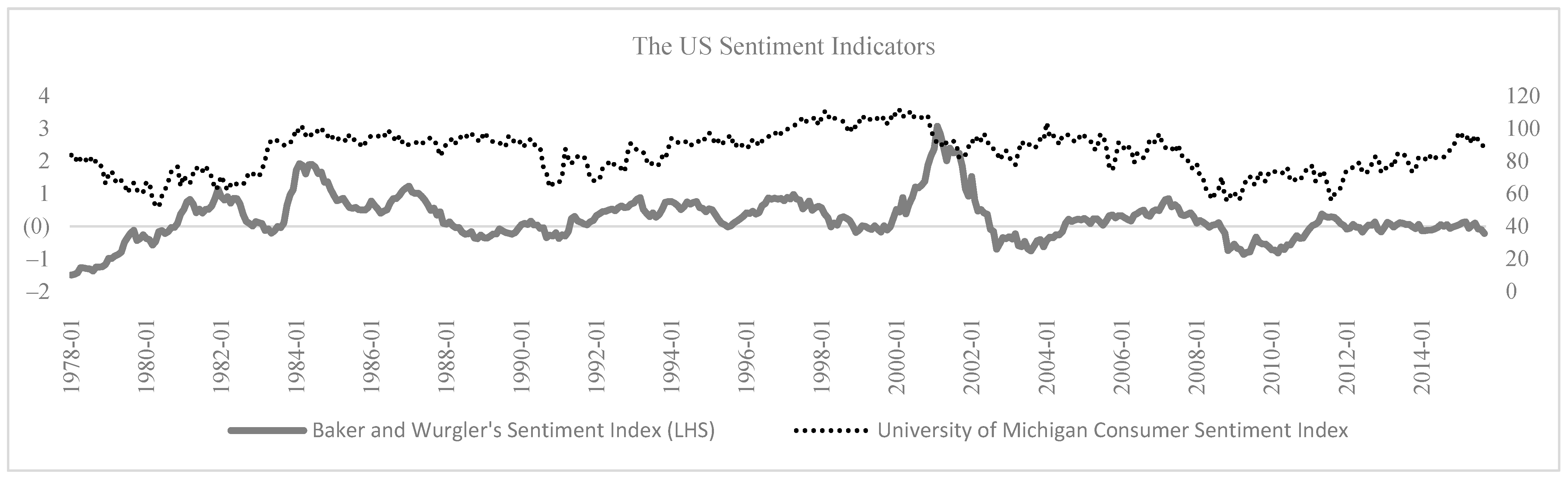
The sentiment indicators’ trajectory is depicted in Figure 1. Baker and Wurgler’s index is more sensitive to stock market fluctuations because it incorporates stock market related variables (the index rose to record high levels prior to the 2001 crisis and then plunged sharply during the crisis). On the other hand, the University of Michigan consumer sentiment index is more prone to consumers’ expectations on general economic conditions.

Table 6. Regression results: constant coefficient (alpha) in the FF3F and FF5F models.

		US		Japan		Europe		North America		Global
Anomaly No	Anomaly	FF3F	FF5F	FF3F	FF5F	FF3F	FF5F	FF3F	FF5F	FF3F	FF5F
1	Size	−0.11	0.05	0.16 *	0.14	−0.02	0.03	0.19 *	0.36 ***	0.22 ***	0.25 ***
		0.24	0.61	0.07	0.11	0.82	0.67	0.08	0.00	0.01	0.00
2	Book-to-market	−0.26 **	−0.06	0.12 *	0.11	0.26 ***	0.12 **	0.29 ***	0.15 **	0.30 ***	0.18 ***
		0.02	0.57	0.10	0.13	0.00	0.01	0.00	0.03	0.00	0.00
3	Momentum	1.61 ***	1.06 ***	0.02	−0.37	1.17 ***	0.68 ***	0.95 ***	0.72 ***	0.96 ***	0.69 ***
		0.00	0.00	0.69	0.31	0.00	0.00	0.00	0.01	0.00	0.00
4	Investments	0.33 **	0.08	0.11	0.05	0.26 ***	0.11 **	0.59 ***	0.36 ***	0.36 ***	0.22 ***
		0.01	0.47	0.37	0.35	0.00	0.02	0.00	0.00	0.00	0.00
5	Operating profitability	0.64 ***	−0.03	0.11	0.05	0.41 ***	−0.33 ***	0.19 *	−0.22 ***	0.14	−0.17 ***
		0.00	0.73	0.27	0.42	0.00	0.00	0.09	0.00	0.04 **	0.00
6	Short-term reversal	−0.11	0.04
		0.67	0.90
7	Long-term reversal	−0.15	−0.05
		0.43	0.76
8	Accruals	0.38 ***	0.38 ***
		0.00	0.00
9	Cashflow/price	0.10	0.00
		0.46	0.99
10	Dividend yield	−0.02	0.02
		0.93	0.92
11	Earnings/price	0.06	−0.05
		0.68	0.73
12	Market beta	0.47 **	0.10
		0.01	0.56
13	Net share issues	0.65 ***	0.30 ***
		0.00	0.01
14	Residual variance	1.27 ***	0.52 ***
		0.00	0.00
15	Variance	1.17 ***	0.37 *
		0.00	0.08

Notes: FF3F and FF5F stand for Fama–French three-factor and Fama–French five-factor models, respectively, and are defined as follows. FF3F: R_it − r_ft = a + b (R_mt −r_ft) + s SMB_t + h HML_t + ε_t and FF5F: R_it − r_ft = a + b (R_mt − r_ft) + s SMB_t+ h HML_t + r RMW_t + c CMA_t + ε_t where t is time subscript, i = 1 to 15 is anomaly strategy, R_i is the return obtained by implementing the anomaly strategy i, r_f is risk-free rate, R_m is market return, SMB (small minus big) is size premium, HML (high minus low) is value premium, RMW (robust minus weak) is the difference between the returns of portfolios composed of stocks with robust and weak profitability, and CMA (conservative minus aggressive) is the return difference of conservative investment portfolios and aggressive investment portfolios. The dataset consists of five countries or regions (US, Japan, Europe, North America and global) and monthly portfolio return data and investor sentiment index data from 1978, 1990, 2004 to 2015, and 2018, depending on the country or region. The US return data are value-weighted. Japan, Europe, North America and global portfolios were calculated using combination portfolios. The figures show the constant coefficient (a) in each regression and the related p-value below. Any significance means that anomaly return has still an unexplained component beyond the factors suggested by the FF3F or FF5F models. *, ** and *** indicate significance at 10%, 5% and 1%, respectively.

provides the constant coefficients (“a” parameter in the regressions, also called “alpha” in common practice) estimated by the regressions suggested by FF3F and FF5F models (Equations (1) and (2), respectively). Alpha refers to excess risk-adjusted return that cannot be explained by the control variables. Any significant alpha reveals that the relevant anomaly return is not fully explained by the factors suggested by the FF3F or FF5F models and could be potentially explained further by adding other variables to the model. The table shows that, in the case of the US, the coefficient is significantly positive for anomaly strategies such as momentum, accruals, net share issues and residual variance (investment, operating profitability, market beta and variance) considering both FF3F and FF5F (considering only FF3F). For other regions, investments is the anomaly for which the coefficient is commonly significant (except Japan) and positive and other anomalies such as size, book-to-market or momentum (in line with Griffin et al. 2003) also reveal significance. These results indicate that many anomalies are still active (as also documented by Liu et al. 2017) and cannot by fully explained by the FF3F and FF5F models.

The figures in the table also signal that, in the US, strategies such as book-to-market, investments, operating profitability, market beta and variance do not produce a significant alpha when FF5F is used instead of FF3F. This finding supports the prevalence of FF5F over FF3F. Meanwhile, the insignificance of certain anomalies may support Schwert (2003), who argued that anomalies may disappear after traders are informed about their existence.

Table 7. Regression results: coefficient of the sentiment change variable in the augmented FF3F and FF5F models.

		US (Baker and Wurgler)		US (U Michigan)		Japan		Europe		North America		Global
An No	Anomaly	FF3F	FF5F	FF3F	FF5F	FF3F	FF5F	FF3F	FF5F	FF3F	FF5F	FF3F	FF5F
1	Size	1.53 ***	1.69 ***	0.06 ***	0.06 ***	0.05	0.05	0.09 **	0.10 **	0.07 **	0.06 **	0.00	−0.00
		0.01	0.01	0.01	0.01	0.35	0.33	0.04	0.03	0.01	0.02	0.99	0.95
2	Book-to-market	0.72	0.88	0.01	0.01	−0.06	−0.04	0.04	0.04	0.00	0.00	−0.00	0.00
		0.31	0.19	0.65	0.67	0.20	0.37	0.25	0.23	0.83	0.76	0.96	0.88
3	Momentum	−0.43	−0.73	−0.18 **	−0.18 **	−0.36 **	−0.23	−0.04	−0.06	−0.18 ***	−0.18 ***	−0.12 **	−0.11 **
		0.84	0.72	0.04	0.03	0.03	0.11	0.75	0.62	0.00	0.00	0.01	0.02
4	Investments	1.32 *	1.27 **	−0.03	−0.02	−0.16 **	0.04	−0.02	0.00	0.02	0.01	−0.00	0.00
		0.10	0.05	0.46	0.49	0.03	0.25	0.65	0.86	0.33	0.37	0.94	0.69
5	Operating profitability	1.55	1.01 *	0.01	0.01	0.11 *	0.05	0.00	−0.02	−0.00	0.01	0.01	0.01
		0.12	0.09	0.76	0.78	0.08	0.19	0.95	0.50	0.96	0.39	0.69	0.33
6	Short-term reversal	1.03	1.10	0.00	0.01
		0.52	0.49	0.93	0.94
7	Long-term reversal	0.40	0.58	−0.03	−0.03
		0.73	0.58	0.47	0.47
8	Accruals	0.81	0.85	−0.01	−0.00
		0.32	0.29	0.88	0.99
9	Cashflow/price	−0.12	−0.22	−0.00	−0.01
		0.89	0.80	0.95	0.87
10	Dividend yield	−0.23	−0.17	−0.03	−0.02
		0.84	0.88	0.59	0.62
11	Earnings/price	0.38	0.27	−0.01	−0.01
		0.66	0.74	0.86	0.78
12	Market beta	−0.46	−0.69	0.02	0.03
		0.68	0.51	0.61	0.51
13	Net share issues	0.93	0.72	−0.01	−0.01
		0.23	0.30	0.79	0.85
14	Residual variance	−0.22	−0.76	−0.06	−0.05
		0.87	0.48	0.30	0.23
15	Variance	0.90	0.35	−0.07	−0.06
		0.54	0.78	0.27	0.23

Notes: Augmented FF3F and augmented FF5F stand for Fama–French 3-factor and Fama–French 5-factor models, respectively, added with a sentiment variable. They are defined as follows. FF3F: R_it − r_ft = a + b (R_mt − r_ft) + s SMB_t + h HML_t + δ ∆S_t + ε_t and FF5F: R_it − r_ft = a + b (R_mt − r_ft) + s SMB_t+ h HML_t + r RMW_t + c CMA_t + δ ∆S_t + ε_t where t is time subscript, i = 1 to 15 is anomaly strategy, R_i is the return obtained by implementing the anomaly strategy i, r_f is risk-free rate, R_m is market return, SMB (small minus big) is size premium, HML (high minus low) is value premium, RMW (robust minus weak) is the difference between the returns of portfolios composed of stocks with robust and weak profitability, CMA (conservative minus aggressive) is the return difference of conservative investment portfolios and aggressive investment portfolios, and S is investor sentiment (measured by U Michigan indices for US as well as North American and global portfolios, CCI for Japanese portfolio and ESI for European portfolio). The dataset consists of five countries or regions (US, Japan, Europe, North America and global) and monthly portfolio return data and investor sentiment index data from 1978, 1990, 2004 to 2015, and 2018, depending on the country or region. The US return data are value-weighted. Japan, Europe, North America and global portfolios were calculated using combination portfolios. The figures show the constant coefficient (a) in each regression and the related p-value parentheses below. *, ** and *** indicate significance at 10%, 5% and 1%, respectively.

provides the coefficient of the sentiment change variable in the regressions based on the augmented FF3F and FF5F models described in Equations (3) and (4), respectively. Any significance in this coefficient (sentiment variable) reveals that sentiment change contributes to explaining anomaly strategy returns. According to the table, sentiment change has a significantly positive coefficient when size strategy returns are used as the dependent variable, regardless of the model (FF3F or FF5F) and geographic region (with the only exceptions of significance being the Japanese and global portfolios). Other results were more heterogenous across regions or sentiment indices. For example, for the US portfolio, when sentiment was measured using the Baker and Wurgler index, sentiment change had a significantly positive impact on investment strategy returns in the case of both FF3F and FF5F models, while this impact disappeared when it as measured using the U Michigan index. For the Japanese portfolio, sentiment change had a significantly positive impact on operating profitability strategy return in the case of FF3F. Across regions, momentum anomaly was the only one for which sentiment change had a negative sign. Under the assumption that momentum stocks are more volatile, this outcome could be explained by the negative relationship between volatile stocks and sentiment since Baker and Wurgler (2006) indicate that when sentiment is low, the subsequent returns are higher for high volatile stocks.

Table 7 does not list constant coefficients (alphas) since our focus is sentiment and the return relationship. Yet, our findings indicate that alphas are still significant when sentiment change is used. In other words, while sentiment change has an impact on anomaly returns, it is not the only answer for excess alpha.

Our findings partially match with the literature. For example, the fact that sentiment is able to explain several anomaly returns is in line with Stambaugh et al. (2012) and Stambaugh and Yuan (2017)5. On the other hand, Stambaugh et al. (2012) only employed a FF3F model whereas we confirmed the results using both FF3F and FF5F models.

4.2. Fixing the Size Factor

In a recent study, Fama and French (2016) examined anomaly returns by controlling (fixing) size factor. Inspired by this study, we examined sentiment’s explanatory power on four different anomalies’ (book-to-market, momentum, investments and operating profitability) returns by fixing the size factor. For this, we defined “combination portfolios” (Pfs 1 to 6 in

Table 8. Combination portfolios based on size and other factors.

	Pf 1	Pf 2	Pf 3	Pf 4	Pf 5	Pf 6
Size	Small	Small	Small	Big	Big	Big
Book-to-market	Low	Mid	High	Low	Mid	High
	Pf 1	Pf 2	Pf 3	Pf 4	Pf 5	Pf 6
Size	Small	Small	Small	Big	Big	Big
Investments	Low	Mid	High	Low	Mid	High
	Pf 1	Pf 2	Pf 3	Pf 4	Pf 5	Pf 6
Size	Small	Small	Small	Big	Big	Big
Operating profitability	Low	Mid	High	Low	Mid	High
	Pf 1	Pf 2	Pf 3	Pf 4	Pf 5	Pf 6
Size	Small	Small	Small	Big	Big	Big
Momentum	Low	Mid	High	Low	Mid	High

Notes: Each portfolio is a binary combination of size and book-to-market value. In the first panel, the first portfolio (Pf 1) consists of stocks with small size and low book-to-market ratio whereas the last portfolio (Pf 6) consists of stocks with big size and high book-to-market ratio. Other panels are analogous.

) that consist of binary combinations of size (small and big) and the relevant anomaly (low, mid and high). Consequently, it is possible to define anomaly strategy return separately for small and large firms simply by subtracting the returns of combination portfolios from each other. For example, the return of Pf 3 minus the return of Pf 1 shows the book-to-market strategy return for small firms and return of Pf 6 minus return of Pf 4 shows the book-to-market strategy return for large firms (analogously for other anomalies).

The results shown in

Table 9. Regression results for the combination portfolios: coefficient of the sentiment change variable in the augmented FF3F model.

Panel A: US	Equally Weighted					Controlling Size Factor
	Sentiment	t-Stat	p-Value	Adj R-Square		Sentiment	t-Stat	p-Value	Adj R-Square
Book-to-market	0.70	0.99	0.32	0.66	When size is small	−0.31	−0.53	0.60	0.67
					When size is big	1.24 ***	3.29	0.00	0.83
Investments	1.99 **	2.41	0.02	0.21	When size is small	1.25 **	2.24	0.03	0.19
					When size is big	0.83	1.64	0.10	0.52
Operating profitability	−1.94 *	−1.77	0.08	0.23	When size is small	−1.54 **	−1.98	0.05	0.17
					When size is big	0.97	1.25	0.21	0.14
Momentum	−0.95	−0.50	0.62	0.02	When size is small	−0.26	−0.20	0.84	0.02
					When size is big	−0.10	−0.07	0.94	0.09
Panel B: Europe	Equally Weighted					Controlling Size Factor
	Sentiment	t-Stat	p-Value	Adj R-Square		Sentiment	t-Stat	p-Value	Adj R-Square
Book-to-market	0.04	1.14	0.25	0.84	When size is small	0.08 *	1.65	0.10	0.59
					When size is big	−0.01	−0.18	0.86	0.78
Investments	−0.02	−0.46	0.65	0.49	When size is small	0.00	0.04	0.97	0.39
					When size is big	−0.04	−0.78	0.44	0.43
Operating profitability	0.00	0.06	0.95	0.11	When size is small	−0.02	−0.36	0.72	0.03
					When size is big	0.02	0.43	0.67	0.21
Momentum	−0.04	−0.32	0.74	0.12	When size is small	−0.10	−0.88	0.38	0.08
					When size is big	0.02	0.16	0.88	0.14
Panel C: Japan	Equally Weighted					Controlling Size Factor
	Sentiment	t-Stat	p-Value	Adj R-Square		Sentiment	t-Stat	p-Value	Adj R-Square
Book-to-market	−0.06	−1.30	0.20	0.85	When size is small	−0.05	−0.50	0.62	0.60
					When size is big	−0.08	−1.26	0.21	0.78
Investments	−0.16 **	−2.17	0.03	0.34	When size is small	−0.14 *	−1.73	0.09	0.34
					When size is big	−0.18 **	−2.06	0.04	0.24
Operating profitability	0.11 *	1.77	0.08	0.35	When size is small	0.09	1.30	0.20	0.41
					When size is big	0.14 *	1.65	0.10	0.19
Momentum	−0.36 **	−2.26	0.03	0.13	When size is small	−0.32 *	−1.97	0.05	0.07
					When size is big	0.40 **	−2.20	0.03	0.14
Panel D: North America	Equally Weighted					Controlling Size Factor
	Sentiment	t-Stat	p-Value	Adj R-Square		Sentiment	t-Stat	p-Value	Adj R-Square
Book-to-market	0.27	0.63	0.53	0.89	When size is small	−0.11	−0.17	0.86	0.80
					When size is big	0.64	1.41	0.16	0.87
Investments	0.99 *	1.68	0.09	0.62	When size is small	1.29 *	1.84	0.07	0.35
					When size is big	0.71	1.04	0.30	0.69
Operating profitability	−0.69	−1.03	0.31	0.42	When size is small	−2.22 ***	−2.94	0.00	0.31
					When size is big	0.85	1.13	0.26	0.44
Momentum	0.11	0.07	0.95	0.10	When size is small	−0.08	−0.05	0.96	0.04
					When size is big	0.29	0.17	0.87	0.14
Panel E: Global Portfolios	Equally Weighted					Controlling Size Factor
	Sentiment	t-Stat	p-Value	Adj R-Square		Sentiment	t-Stat	p-Value	Adj R-Square
Book-to-market	0.02	0.06	0.95	0.90	When size is small	−0.46	−1.20	0.23	0.79
					When size is big	0.49	1.42	0.16	0.85
Investments	0.47	1.22	0.22	0.64	When size is small	0.50	1.22	0.22	0.43
					When size is big	0.44	0.92	0.36	0.67
Operating profitability	−0.12	−0.30	0.76	0.37	When size is small	−0.99 **	−2.22	0.03	0.25
					When size is big	0.75	1.60	0.11	0.37
Momentum	0.64	0.54	0.59	0.13	When size is small	0.74	0.66	0.51	0.08
					When size is big	0.54	0.40	0.69	0.16

Notes: Augmented FF3F stands for Fama–French three-factor model, added with a sentiment change variable. It is defined as follows FF3F: R_it − r_ft = a + b (R_mt − r_ft) + s SMB_t + h HML_t + ε_t, where t is time subscript, i = 1 to 15 is anomaly strategy, R_i is the return obtained by implementing the anomaly strategy i, r_f is risk-free rate, R_m is market return, SMB (small minus big) is size premium, HML (high minus low) is value premium, and S is investor sentiment (measured using Baker and Wurgler index for US as well as North American and global portfolios, CCI for Japanese portfolio and ESI for European portfolio). The dataset consists of five countries or regions (US, Japan, Europe, North America and global) and monthly portfolio return data and investor sentiment index data from 1978, 1990, 2004 to 2015, and 2018, depending on the country or region. The US return data are value-weighted. Japan, Europe, North America and global portfolios were calculated using combination portfolios. The figures show the constant coefficient (a) in each regression and the related p-value below. *, ** and *** indicate significance at 10%, 5% and 1%, respectively.

indicate that for investment strategy, the coefficient for the US portfolios is significantly positive. Yet, when separately analyzed, one can notice that this is rather the case for small stocks while the evidence for large-size stocks does not exist.

Considering overall stocks on the left halves of the panels, the coefficients of other anomaly returns were not systematically significant. However, when size factor was controlled, the results changed markedly. For example, concerning the momentum strategy returns in Japanese portfolios, the coefficients were significantly negative (positive) for small (large) stocks. It appears that momentum anomaly returns are negatively related with sentiment change when small stocks are used. Additionally, in the case of the US portfolio, the coefficients (sentiment change) for operating profitability were significantly negative for small stocks yet insignificant for large stocks. However, this result held only for the US and North America portfolios.

These findings show that sentiment change helps to explain investments and operating profitability anomaly returns. A deeper analysis reveals that the size factor plays a key role in anomaly returns. Yang et al. (2017) argued that sentiment has stronger impact on stocks with lower market capitalization. Moreover, Bathia and Bredin (2013) indicated that value stocks’ returns in G7 countries are more prone to the sentiment effect. We confirmed that stock characteristics are important to the explanatory power of sentiment for investments anomaly in the US, Europe and North America.

4.3. Robustness Checks

4.3.1. Combination Portfolios Instead of Portfolios Formed Based on a Single Anomaly

In the previous section, we used combination portfolios for regions other than the US not only for fixing one factor but also due to the lack of pure anomaly strategy return data. These two-dimensional feature of anomaly returns (e.g., book-to-market anomaly returns when stock size is small or big) are used to proxy for anomaly returns. For example, referring to the upper part of Table 8 (regarding size and book-to-market), averaging the returns of Pf 1 and Pf 4 would provide the return of a pure low book-to-market strategy while averaging the returns of Pf 3 and Pf 6 would provide the return of a pure high book-to-market strategy (with the difference that portfolios composed in this way are equally weighted instead of being value-weighted). Effectively, the effect of size becomes neutralized. Then, subtracting the former from the latter (high minus low) provides the book-to-market anomaly return (analogously for investment, operating profitability and momentum strategies). Hence, we performed an alternative analysis and check for whether this method yielded the same findings for the pure strategy returns found in Section 4.1.

On Kenneth French’s data library6, only nine different anomaly portfolios were available in combination format for the US market. Among these portfolios, five strategies (size, book-to-market, investment, operating profitability, and momentum) were examined for Europe, Japan, North America and global markets7. We calculated the anomaly returns as explained above and tested the relation between anomalies and the investor sentiment measure.

As

Table 10. Using combination portfolios for US data.

	Equally Weighted				Combination Portfolio
Anomalies	Sentiment	t-Stat	p-Value	Adj R-Square	Sentiment	t-Stat	p-Value	Adj R-Square
Size	2.84 ***	3.16	0.00	0.59	1.37 **	2.22	0.03	0.59
Book-to-market	0.70	0.99	0.32	0.66	0.46	1.29	0.20	0.84
Momentum	−0.95	−0.50	0.62	0.02	−0.18	−0.14	0.89	0.05
Investments	1.99 **	2.41	0.02	0.21	1.04 **	2.47	0.01	0.45
Operating profitability	−1.94 *	−1.77	0.08	0.23	−0.29	−0.41	0.68	0.16

Notes: Three-factor model was used in this test (Fama and French 1993). Rt − rft = α + β (Rm − rf)t + s(SMB)t + h(HML)t + δ ∆ (S)t + ε, where Ri is return of the anomaly strategy, rf is risk-free rate, Rm − rf is the difference between rf and return of value-weighted market portfolio, SMB is size premium, HML is value premium, and S is sentiment. Sentiment measure refers to Baker and Wurgler (2006). Parameter estimate belongs to sentiment variable. *, ** and *** indicate significance at 10%, 5% and 1%, respectively.

indicates, anomaly strategies calculated from combination portfolios have a similar relationship with single anomaly portfolios composed of 10 deciles at the 5% significance level. This finding supports our intention to use combination portfolios for Europe, Japan, North America and global markets in anomaly research.

4.3.2. Using Equally Weighted Portfolios Instead of Value-Weighted Portfolios

It can be argued that value-weighted portfolios are more meaningful in examining the relationship between sentiment and anomaly returns. Followingly, we check whether choosing a value-weighted or equally weighted portfolio really makes a difference as to the relationship between sentiment and anomaly returns8.

The results shown in

Table 11. Value-weighted vs equally weighted portfolios (US data).

	Equally Weighted				Value-Weighted
Anomalies	Sentiment	T-Stat	p-Value	Adj R-Square	Sentiment	t-Stat	p-Value	Adj R-Square
Size	2.84 ***	3.16	0.00	0.59	1.53 ***	2.78	0.01	0.83
Book-to-market	0.70	0.99	0.32	0.66	0.72	1.02	0.31	0.74
Momentum	−0.95	−0.50	0.62	0.02	−0.42	−0.20	0.84	0.07
Short-term reversal	2.62 *	1.76	0.08	0.07	1.02	0.65	0.52	0.09
Long-term reversal	2.64 **	2.24	0.03	0.23	0.40	0.35	0.73	0.34
Accruals	1.08 **	2.20	0.03	0.02	0.81	1.00	0.32	0.02
Cashflow/price	0.18	0.30	0.77	0.54	−0.11	−0.13	0.89	0.47
Dividend yield	0.57	0.67	0.50	0.46	−0.23	−0.20	0.84	0.53
Earnings/price	0.14	0.23	0.82	0.55	0.38	0.44	0.66	0.51
Investments	1.99 **	2.41	0.02	0.21	1.32 *	1.66	0.10	0.29
Market beta	−1.56	−1.59	0.11	0.65	−0.46	−0.41	0.68	0.67
Net share issues	−0.47	−0.54	0.59	0.40	0.93	1.21	0.23	0.31
Operating profitability	−1.94 *	−1.77	0.08	0.23	1.55	1.57	0.12	0.39
Residual variance	−1.81	−1.34	0.18	0.57	−0.22	−0.17	0.87	0.65
Variance	−1.40	−1.02	0.31	0.58	0.89	0.61	0.54	0.63

Notes: Three-factor model was used in this test (Fama and French 1993). Rt − rft = α + β (Rm − rf)t + s(SMB)t + h(HML)t + δ ∆ (S)t + ε, where Ri is return of the anomaly strategy, rf is risk-free rate, Rm − rf is the difference between rf and return of value-weighted market portfolio, SMB is size premium, HML is value premium and S is sentiment. Sentiment measure refers to Baker and Wurgler (2006). Parameter estimate belongs to sentiment variable. *, ** and *** indicate significance at 10%, 5% and 1%, respectively.

indicate that the sign and significance of the sentiment change coefficient for different anomalies do not really change across the two types of portfolios at 1% significance. These results provide support for Stambaugh et al. (2012) and Jacobs (2015), who found that equally weighted and value-weighted anomaly portfolios attain similar results.

4.3.3. Examining Size Anomaly While Controlling Other Factors

We wondered whether size anomaly is related with sentiment when some factors are constant. In order to test this, we regressed size anomalies by fixing one factor.

Table 12. Examining size anomaly while controlling other factors (US data).

	Size Anomaly with Different Stock Characteristics
	Sentiment	t-Stat	p-Value	Adj R-Square
When book-to-market is low	2.39 ***	2.96	0.00	0.52
When book-to-market is medium	0.87	1.55	0.12	0.62
When book-to-market is high	0.84	1.18	0.24	0.50
When investment is low	2.25 **	2.50	0.01	0.48
When investment is medium	0.54	1.11	0.27	0.62
When investment is high	1.84 ***	2.80	0.00	0.47
When operating profit is low	2.73 ***	3.08	0.00	0.38
When operating is medium	0.23	0.51	0.61	0.58
When operating profit is high	0.22	0.46	0.64	0.65
When momentum is low	1.32	1.27	0.21	0.36
When momentum is medium	0.65	1.38	0.17	0.60
When momentum is high	1.16 **	2.00	0.05	0.46
Size anomaly	2.84 ***	3.16	0.00	0.59

Notes: Three-factor model was used in this test (Fama and French 1993). Rt – rft = α + β (Rm – rf)t + s(SMB)t + h(HML)t + δ ∆ (S)t + ε, where Ri is return of the anomaly strategy, rf is risk-free rate, Rm − rf is the difference between rf and return of value-weighted market portfolio, SMB is size premium, HML is value premium, and S is sentiment. Sentiment measure refers to Baker and Wurgler (2006). Parameter estimate belongs to sentiment variable. ** and *** indicate significance at 5% and 1%, respectively.

shows that size anomaly and sentiment have a predictive relationship when stocks’ book-to-market and operating profit factors are low and momentum is high. The latter part of Table 12 lists results regarding the size anomaly and sentiment relationship without controlling any factor. Hence, fixing factors other than size may be important in the sentiment and anomaly relationship.

4.3.4. Calculating Size Anomaly Returns from Various Combination Portfolios

In this study, we defined various anomaly returns using combination portfolios. For example, referring to the upper part of Table 8, the average return of Pf 1, Pf 2 and Pf 3 minus the average return of Pf 4, Pf 5 and Pf 6 provides the return for size anomaly (small minus big) using book-to-market portfolios. Yet, size anomaly return can be also obtained by combining size with investments, operating profitability and momentum portfolios. Whether alternative combinations to calculate a certain anomaly return provide the same result as for the relationship between sentiment change and relevant anomaly returns remains an open question.

Table 13. Regression results: coefficient of sentiment change in the augmented FF3F model when size anomaly return is calculated with alternative combinations.

	Parameter Estimate	t-Stat	p-Value	Adj R-Square
Panel A: European Portfolios
Size strategy return from book-to-market combination	0.09 **	2.03	0.04	0.66
Size strategy return from investment combination	0.09 **	2.01	0.05	0.66
Size strategy return from operating profit combination	0.11 ***	2.61	0.01	0.69
Size strategy return from momentum combination	0.08 *	1.65	0.10	0.62
Panel B: Japanese Portfolios
Size strategy return from book-to-market combination	0.05	0.93	0.35	0.75
Size strategy return from investment combination	0.04	0.77	0.44	0.75
Size strategy return from operating profit combination	0.04	0.67	0.51	0.74
Size strategy return from momentum combination	0.11 *	1.96	0.05	0.67
Panel C: North America Portfolios
Size strategy return from book-to-market combination	2.01 ***	3.13	0.00	0.64
Size strategy return from investment combination	1.89 ***	3.12	0.00	0.59
Size strategy return from operating profit combination	1.29 **	2.49	0.01	0.62
Size strategy return from momentum combination	1.73 ***	2.69	0.01	0.51
Panel D: Global Portfolios
Size strategy return from book-to-market combination	1.67 ***	3.53	0.00	0.60
Size strategy return from investment combination	1.57 ***	3.48	0.00	0.58
Size strategy return from operating profit combination	1.27 ***	3.05	0.00	0.61
Size strategy return from momentum combination	1.43 ***	2.99	0.00	0.53

Notes: Three-factor model was used in this test (Fama and French 1993). Rt − rft = α + β (Rm − rf)t + s(SMB)t + h(HML)t + δ ∆ (S)t + ε, where Ri is return of the anomaly strategy, rf is risk-free rate, Rm − rf is the difference between rf and return of value-weighted market portfolio, SMB is size premium, HML is value premium, and S is sentiment. For North America and global portfolios, sentiment measure refers to Baker and Wurgler (2006). Parameter estimate belongs to sentiment variable. *, ** and *** indicate significance at 10%, 5% and 1%, respectively.

shows the coefficient of sentiment change variable in the FF3F based regression model to explain size anomaly return for different geographic regions. According to the table, even if the sign and significance of the coefficients may vary across regions (e.g., they are insignificant except for Europe), they remain the same across combinations (within each panel). Hence, we concluded that calculating anomaly returns using different combinations does not matter.

5. Conclusions

Price anomalies have long been investigated in the finance literature. However, whether they can be explained by investor sentiment in addition to other existing asset pricing models remains open to debate. Motivated by this fact, we conducted an analysis on stock portfolios representing various geographic locations (US, Europe, Japan, North America and global). Our dataset extends to 1978, 1990, 2004 to 2015, and 2018, depending on the country or region. We examined the existence of anomalies, explained these anomalies with sentiment indicators and assessed whether the explanatory power of sentiment depends on size factor.

Our evidence shows that anomalies exist in the US stock market when tested using the Fama–French three-factor (FF3F) and Fama–French five-factor (FF5F) models. We also asserted that momentum, accruals, net share issues and residual variance strategies produce higher returns than risk-adjusted returns. Additionally, in the US market, size, investments and operating profitability anomalies were predicted using Baker and Wurgler’s investor sentiment index. On the other hand, the University of Michigan consumer sentiment index explained only returns of size and momentum anomalies. Hence, we conclude that indirect sentiment indicators perform better in this aspect.

Investor sentiment’s power in anomaly explanations is valid not only in the US but also in the Europe, Japan and global portfolios. Therefore, investor sentiment’s explanatory power might be universal, but it changes on the basis of anomalies. Additionally, the explanatory power of sentiment changes when the size factor is fixed. In other words, the impact of sentiment on returns is related to market capitalization. For instance, sentiment can explain investment anomaly in US portfolios. However, when separately analyzed, one might notice that this is rather the case for small stocks but not for large stocks. Our findings and the method (using combination portfolios) were supported by robustness checks.

Our study has several implications. First, preference for indirect sentiment indicators over direct ones may improve prediction models both in academia and practice. Secondly, asset managers who follow factor-investing strategies can consider the impact of the size factor. For example, for book-to-market strategy, picking larger stocks when sentiment is expected to rise might result in higher returns. On the other hand, the opposite method of trading is valid for investment strategy.

Our study offers new ground for anomaly research by fixing the stock characteristics when analyzing the effect of sentiment. Additionally, creating pure anomaly returns from combination portfolios is a new practice that could potentially gain traction.

As further research, the relationship between sentiment and anomaly should be examined in other parts of the world and with different types of investor sentiment indicators. Note that indirect indicators seem a better choice for this analysis. Furthermore, referring to Bathia and Bredin (2013), Yang et al. (2017) and our findings in Section 4.3.3. (i.e., examining the size anomaly while controlling other factors), anomaly and sentiment relationship can be examined by fixing other factors such as book-to-market ratio and volatility.

References

- Ali, Ashiq, and Umit G. Gurun. 2009. Investor Sentiment, Accruals Anomaly, and Accruals Management. Journal of Accounting, Auditing & Finance 24: 415–31. [Google Scholar]
- Altanlar, Ali, Jiaqi Guo, and Phil Holmes. 2019. Do culture, sentiment, and cognitive dissonance explain the “above suspicion” anomalies? European Financial Management 25: 1168–95. [Google Scholar] [CrossRef]
- Ang, Andrew, Robert J. Hodrick, Yuhang Xing, and Xiaoyan Zhang. 2006. The cross-section of volatility and expected returns. Journal of Finance 61: 259–99. [Google Scholar] [CrossRef] [Green Version]
- Baker, Malcolm, and Jeffrey Wurgler. 2006. Investor Sentiment and the Cross-Section of Stock Returns. Journal of Finance 61: 1645–80. [Google Scholar] [CrossRef] [Green Version]
- Baker, Malcolm, Jeffrey Wurgler, and Yu Yuan. 2012. Global, local, and contagious investor sentiment. Journal of Financial Economics 104: 272–87. [Google Scholar] [CrossRef] [Green Version]
- Banz, Rolf W. 1981. The relationship between return and market value of common stocks. Journal of Financial Economics 9: 3–18. [Google Scholar] [CrossRef] [Green Version]
- Basu, Sanjoy. 1977. Investment Performance of Common Stocks in Relation to Their Price-Earning Ratios: A Test ofthe Efficient Market Hypothesis. Journal of Finance 32: 663–82. [Google Scholar] [CrossRef]
- Basu, Sanjoy. 1983. The Relationship between Earnings’ Yield, Market Value and Return for NYSE Common Stocks: Further Evidence. Journal of Financial Economics 12: 129–56. [Google Scholar] [CrossRef]
- Bathia, Deven, and Don Bredin. 2013. An examination of investor sentiment effect on G7 stock market returns. The European Journal of Finance 19: 909–37. [Google Scholar] [CrossRef]
- Brown, Gregor. W., and Michael T. Cliff. 2005. Investor Sentiment and Asset Valuation. The Journal of Business 78: 405–40. [Google Scholar] [CrossRef]
- Calluzzo, Paul, Fabio Moneta, and Selim Topaloglu. 2019. When Anomalies Are Publicized Broadly, Do Institutions Trade Accordingly? Management Science 65: 4555–74. [Google Scholar] [CrossRef] [Green Version]
- Chan, Louis K. C., Yasushi Hamao, and Josef Lakonishok. 1991. Fundamentals and stock returns in Japan. Journal of Finance 46: 1739–64. [Google Scholar] [CrossRef]
- Chen, Long, Robert Novy-Marx, and Lu Zhang. 2011. An Alternative Three-Factor Model. Available online: https://ssrn.com/abstract=1418117 (accessed on 15 January 2020).
- Cooper, Michael J., Huseyin Gulen, and Michael J. Schill. 2008. Asset Growth and the Cross Section of Stock Returns. Journal of Finance 63: 1069–652. [Google Scholar] [CrossRef]
- Daniel, Kent, and Sheridan Titman. 2006. Market reactions to tangible and intangible information. Journal of Finance 61: 1605–43. [Google Scholar] [CrossRef] [Green Version]
- De Bondt, Werner F. M., and Richard Thaler. 1985. Does the stock market overreact? Journal of Finance 40: 793–805. [Google Scholar] [CrossRef]
- De Bondt, Werner F. M., and Richard H. Thaler. 1987. Further evidence on investor overreaction and stock market seasonality. Journal of Finance 42: 557–81. [Google Scholar] [CrossRef]
- Fama, Eugene F., and Kenneth R. French. 1992. The Cross-Section of Expected Stock Returns. Journal of Finance 47: 427–65. [Google Scholar] [CrossRef]
- Fama, Eugene F., and Kenneth R. French. 1993. Common risk factors in the returns on stocks and bonds. Journal of Financial Economics 33: 3–56. [Google Scholar] [CrossRef]
- Fama, Eugene F., and Kenneth R. French. 2015. A five-factor asset pricing model. Journal of Financial Economics 116: 1–22. [Google Scholar] [CrossRef] [Green Version]
- Fama, Eugene F., and Kenneth R. French. 2016. Disecting Anomalies with a Five-Factor Model. The Review of Financial Studies 29: 69–103. [Google Scholar] [CrossRef]
- Ferreira, Paulo, and Andreia Dionísio. 2014. Revisiting serial dependence in the stock markets of the G7 countries, Portugal, Spain and Greece. Applied Financial Economics 24: 319–31. [Google Scholar] [CrossRef]
- Frazzini, Andrea, and Lasse Heje Pedersen. 2014. Betting against beta. Journal of Financial Economics 111: 1–25. [Google Scholar] [CrossRef] [Green Version]
- Griffin, John M., Xiuqing Ji, and J. Spencer Martin. 2003. Momentum investing and business cycle risk: Evidence from pole to pole. Journal of Finance 58: 2515–47. [Google Scholar] [CrossRef]
- Hackel, Kenneth S., Joshua Livnat, and Atul Rai. 2000. A Free Cash Flow Investment Anomaly. Journal of Accounting, Auditing & Finance 15: 1–24. [Google Scholar]
- Han, Chunmao, and Yongdong Shi. 2022. Chinese stock anomalies and investor sentiment. Pacific-Basin Finance Journal 73: 101739. [Google Scholar] [CrossRef]
- Jacobs, Heiko. 2015. What explains the dynamics of 100 anomalies? Journal of Banking and Finance 57: 65–85. [Google Scholar] [CrossRef]
- Jacobs, Heiko, and Sebastian Müller. 2019. Anomalies across the globe: Once public, no longer existent? Journal of Financial Economics 135: 213–30. [Google Scholar] [CrossRef]
- Jegadeesh, Narasimhan. 1990. Evidence of predictable behavior of security returns. Journal of Finance 45: 881–98. [Google Scholar] [CrossRef]
- Jegadeesh, Narasimhan, and Sheridan Titman. 1993. Returns to buying winners and selling losers: Implications for stock market efficiency. Journal of Finance 48: 65–91. [Google Scholar] [CrossRef]
- Jiang, Lei, Jinyu Liu, Lin Peng, and Baolian Wang. 2021. Investor Attention and Asset Pricing Anomalies. Review of Finance 26: 563–93. [Google Scholar] [CrossRef]
- Keim, Donald B. 1983. Size-related anomalies and stock return seasonality: Further empirical evidence. Journal of Financial Economics 12: 13–32. [Google Scholar] [CrossRef]
- Kim, Dongcheol, and Haejung Na. 2018. Investor Sentiment, Anomalies, and Macroeconomic Conditions. Asia-Pacific Journal of Financial Studies 47: 751–804. [Google Scholar] [CrossRef]
- Lee, Wayne Y., Christine X. Jiang, and Daniel C. Indro. 2002. Stock market volatility, excess returns, and the role of investor sentiment. Journal of Banking and Finance 26: 2277–99. [Google Scholar] [CrossRef]
- Loughran, Tim, and Jay R. Ritter. 1995. The new issues puzzle. Journal of Finance 50: 23–51. [Google Scholar] [CrossRef]
- Lu, Xiaomeng, Robert F. Stambaugh, and Yu Yuan. 2017. Anomalies Abroad: Beyond Data Mining (No. w23809). National Bureau of Economic Research. Available online: https://www.nber.org/papers/w23809 (accessed on 15 January 2020).
- Naranjo, Andy, M. Nimalendran, and Mike Ryngaert. 1998. Stock Returns, Dividend Yields, and Taxes. Journal of Finance 53: 2029–57. [Google Scholar] [CrossRef]
- Narayan, Paresh Kumar, and Susan Sunila Sharma. 2015. Does data frequency matter for the impact of forward premium on spot exchange rate? International Review of Financial Analysis 39: 45–53. [Google Scholar] [CrossRef]
- Narayan, Paresh Kumar, Huson Ali Ahmed, and Seema Narayan. 2015. Do momentum-based trading strategies work in the commodity futures markets? Journal of Futures Market 35: 868–91. [Google Scholar] [CrossRef]
- Reinganum, Marc R. 1983. The anomalous stock market behavior of small firms in January: Empirical tests for tax-loss selling effects. Journal of Financial Economics 12: 89–104. [Google Scholar] [CrossRef]
- Salur, Bayram Veli, and Cumhur Ekinci. 2023. Can Investor Sentiment Indicators Based on Fund Flows and Stock Intensity Predict Stock Returns? Unpublished Working Paper. Istanbul: Istanbul Technical University. [Google Scholar]
- Schwert, G. William. 2003. Anomalies and Market Efficiency. In Handbook of Economics of Finance. Edited by George Constantinides, Milton Harris and René M. Stulz. Amsterdam: Elsevier, pp. 939–74. [Google Scholar]
- Sloan, Richard G. 1996. Do stock prices fully reflect information in accruals and cash flows about future earnings? The Accounting Review 71: 289–315. [Google Scholar]
- Stambaugh, Robert F., and Yu Yuan. 2017. Mispricing Factors. The Review of Financial Studies 30: 1270–315. [Google Scholar] [CrossRef] [Green Version]
- Stambaugh, Robert F., Jianfeng Yu, and Yu Yuan. 2012. The short of it: Investor sentiment and anomalies. Journal of Financial Economics 104: 288–302. [Google Scholar] [CrossRef] [Green Version]
- Yang, Heejin, Doojin Ryu, and Doowon Ryu. 2017. Investor sentiment, asset returns and firm characteristics: Evidence from the Korean Stock Market. Investment Analysts Journal 46: 132–47. [Google Scholar] [CrossRef]
- Zaremba, Adam. 2016. Investor sentiment, limits on arbitrage, and the performance of cross-country stock market anomalies. Journal of Behavioral and Experimental Finance 9: 136–63. [Google Scholar] [CrossRef]
Figure 1.
The US sentiment indicators. Note: The figure illustrates the most widely used sentiment indicators: Baker and Wurgler’s sentiment index and University of Michigan consumer sentiment index. Both indices were measured on a monthly basis. Left axis shows values of Baker and Wurgler’s index and right axis shows values of University of Michigan consumer sentiment index.