Article

Digitalization and Quantitative Flow Visualization of Surrounding Flow over a Specially-Shaped Column-Frame by Luminescent Mini-Tufts Method

1
Institute of Engineering Thermophysics, Chinese Academy of Sciences, Beijing 100190, China
2
School of Astronautics and Aeronautics, University of Chinese Academy of Sciences, Beijing 100049, China
3
Innovation Academy for Light-Duty Gas Turbine, Chinese Academy of Sciences, Beijing 100190, China
*
Author to whom correspondence should be addressed.
Aerospace 2022, 9(9), 507; https://doi.org/10.3390/aerospace9090507
Submission received: 23 June 2022 / Revised: 30 July 2022 / Accepted: 7 September 2022 / Published: 11 September 2022
(This article belongs to the Special Issue Advanced Flow Diagnostic Tools)

Abstract

:
The luminescent mini-tufts method is widely used for flow visualization for quantitative field analysis. A set of numerical methods for digitalization of 3D surfaces surrounding flows with luminescent mini-tufts has been developed in this study. The procedure includes digital image pre-processing, mini-tufts recognition, mean field mini-tufts calculation, inclination angle calculation, oscillation area calculation, etc. The model is subjected to a newly proposed digitalization method and realized by in-house code. The time mean angle’s changing mode, along the mini-tuft, are analyzed, which shows that the mini-tuft follows the inflow well. The transient oscillation of mini-tufts is observed as well, which shows that on the middle part of the irregularity cylinder, the flow oscillates more intensively.

1. Introduction

The luminescent mini-tufts method is one of the most useful techniques of flow visualization [1,2]. This method was proposed firstly in 1979 in order to visualize air tunnel flow. The key point of this method is to attach extremely thin nylon mono-filament fibers, which have been treated with fluorescent dye, onto the surface of the target physical model. By using ultraviolet light, mini-tufts are visible and can be recorded with photography [3]. This method is widely applied in aircraft design, wing testing, rotor/propeller design, automobile design, etc. [4,5,6,7,8,9,10,11,12]. It is a typical method that combines high resolution computer-aided techniques and flow measurement [13]. In recent years, researchers used high-speed cameras to take plenty of snapshots to record the changes in flow characteristics over time. In this study, an attempt is made to recognize the mini-tufts from the snapshots based on which quantitative analysis of flow is performed.
Flow visualization plays a key role in experimental fluid mechanics. Flow visualization has existed as long as fluid flow research itself [14,15]. If flow could be visible, it would be possible to observe flow phenomena, which is essential for researchers to do predictions and numerical simulations through flow dynamic data [16,17,18]. Typical flow visualization methods can be classified into two types: one is surface visualization, while the other is off-surface visualization. The first type includes tufts, fluorescent dye, oil, and special clay mixtures, which are applied on the surface of a target model [19]. Some traces are used in off-surface visualization, such as smoke particles, oil droplets, and helium-filled soap bubbles [20,21]. For all flow visualization methods, an appropriate approach to record the image, such as taking photos or recording videos, is necessary. Profiting from computer techniques, it is possible to analyze flow visualization automatically and achieve qualitative and quantitative information by digital image processing [22,23], which is not easy for conventional flow measurements [24,25,26,27].
Vey et al. [28] established a measurement technique which allows extracting quantitative data from tuft flow visualization on real-world wind turbine blades. Bonitz et al. [29] applied Vey’s approach on the flow interaction characteristics analysis between the wheel, wheelhouse, and the rotation of the wheel of a passenger car. Chen et al. [30] analyzed the steady flow characterization and quantitative flow conducted on a flat plate model with the luminescent mini-tufts method.
In order to ensure visualization and minimize the impact on flow, the diameter of the fluorescent fiber is usually set at 0.01–0.1 mm. However, due to the weak reflected-light, it is hardly visible if the diameter of the mini-tuft is smaller than 0.1 mm. Long exposure time cannot help on that [20].
In this study, flow surrounding a 3D irregular cylinder model is analyzed quantitatively base on the luminescent mini-tufts method. The process includes tuft digitalization and recognition, tuft angle calculation, and tuft oscillation analysis according to its oscillation area. The tuft recognition process is highlighted in this paper, which automatically converts multiple snapshots of luminescent mini-tufts to digital matrixes. The details are given in the following sections.

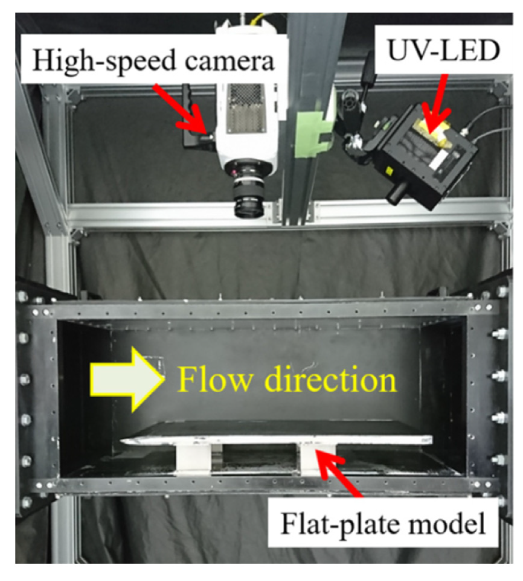
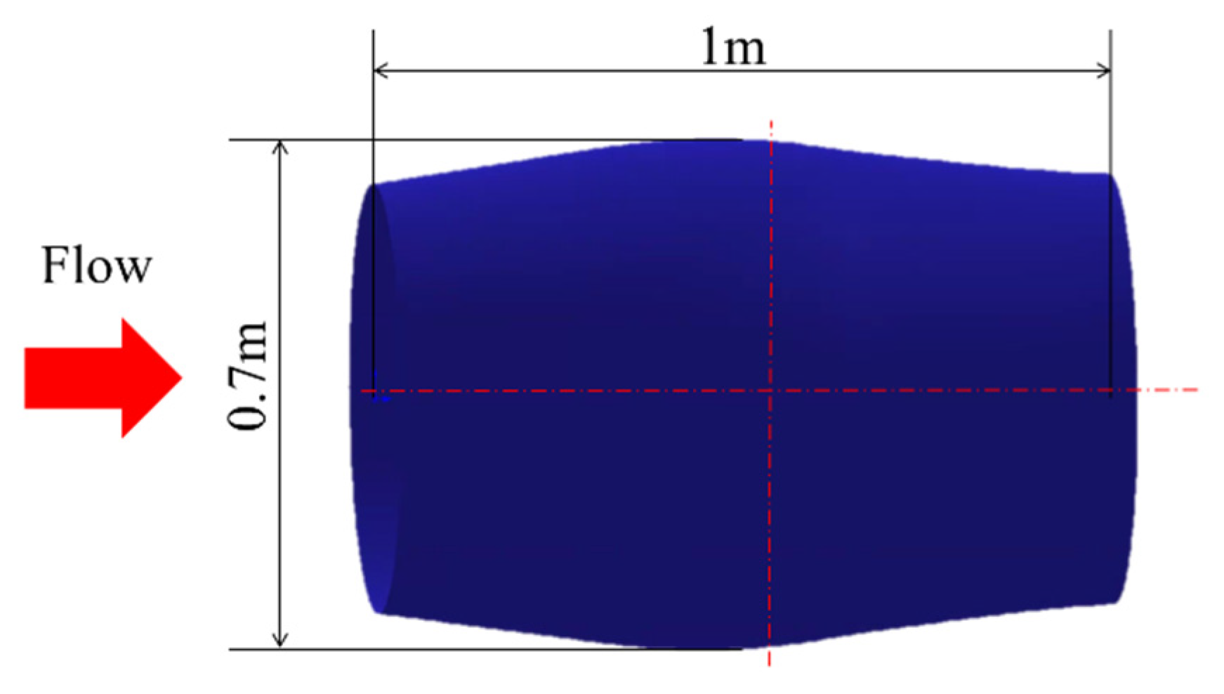
2. Experimental Set-Ups

Experiment and Model

As shown in Figure 1, the experimental set-up in this study is similar to that in reference [30]. Excitation UV light source and high-speed camera are placed on top of the test section, while the target model is mounted inside the visualization section.
In this study, the target model is an irregular metal cylinder from an aircraft engine, as shown in Figure 2. The model’s front surface is laid fully with luminescent mini-tufts. The cylinder model is thin at both ends while thick in the middle. The diameter of its thickest part is 0.7 m. The width is 1 m.
In the experiment, the irregular cylinder model is placed in a dark space with the temperature at 190 K. Wind flow direction is from left to right with velocity 102 m/s. In different experiments, the mini-tufts are attacked by the incoming flow with 3 different angles: 4°, 0°, and −4°. Figure 3 shows the snapshots which plot surrounding flow curve reflected by the luminescent mini-tufts on the 3D model. As it is shown, there are 96 mini-tufts on the front surface of the cylinder. The mini-tufts used in this study were prepared by our experimental center, using bright silk as the base material.
Due to the structure of the irregular cylinder model, as shown in Figure 3, the brightness of each luminescent mini-tuft in one image is not the same. The brightness of each image is also not the same because of the minor change in the environment. Furthermore, the real situation of fluorescent mini-tufts cannot be fully recovered by the highlighted pixels on the image because the area of light is larger than that of fluorescent mini-tufts. The above situations bring great difficulties to the flow analysis using the fluorescent mini-tufts method.

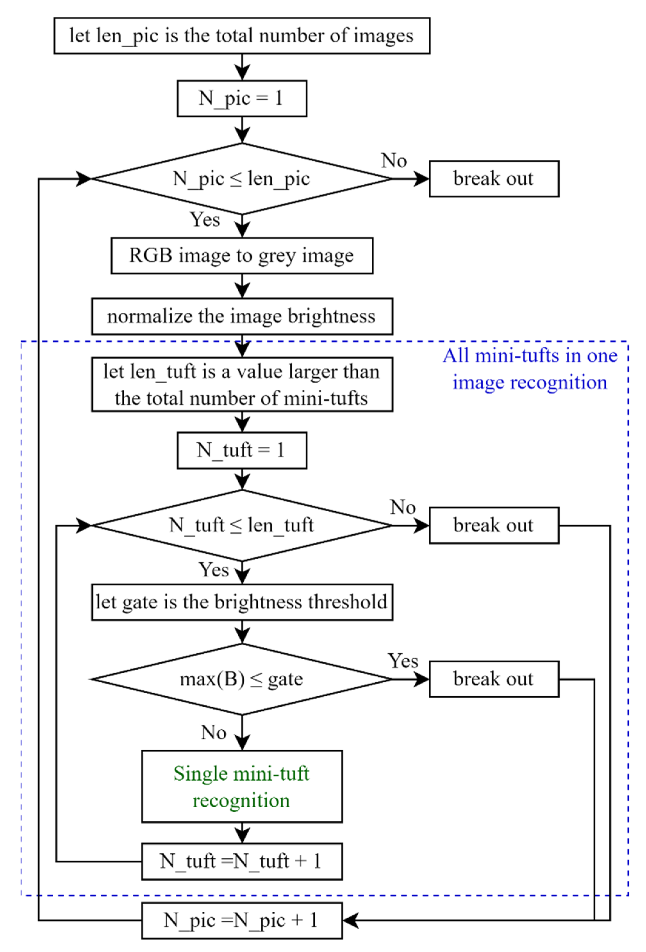
3. Data Processing Method

As mentioned above, with the snapshots of the luminescent mini-tufts, the flow characteristics can be analyzed quantitatively. The first step is to recognize the mini-tufts correctly. In this section, an image processing approach is proposed that can transfer luminescent mini-tufts from snapshots to a digital matrix. The coding process flow is shown in Figure 4.
Figure 4 illustrates the processing of a sequence of images. For each image, all mini-tufts are recognized one by one, and each mini-tuft is recognized individually. The detailed process of each single luminescent mini-tuft recognition is described below.
The main idea of the recognition process is to recognize the luminescent mini-tufts by finding the brightest points in the photos. As it is shown in Figure 4, the first step is to transfer RGB image to grey image. The RGB image in digital span is a 2D matrix whose size is equal to the size of image pixels and every entry has three parameters describing colors, while every entry of the digital matrix of grey image needs only one parameter to describe the brightness. The only brightness parameter of the grey image pixels can be more easily compared in order to recognize the points where mini-tufts locate and expand.
Since the brightness of these 20 photos is not the same, the brightness of different photos should be normalized. In the digital matrix of a grey image, the brighter the point is, lager the entry value will be. In the absolute dark area, the entry values are 0. Find the largest entry in the total 20 grey images which are taken from the experiment:
A = max ( max ( B 1 ) , max ( B 2 ) , , max ( B N _ p i c ) , , max ( B 20 ) )
where BN_pic is the matrix of the number N_pic grey image.
The largest entry in the 20 grey images is 230. The normalized grey image can be obtained as below.
B N _ p i c n o r m a l i z e d = A × B N _ p i c max ( B N _ p i c )
All the mini-tufts in one image are recognized one by one from left to right according to the location of every mini-tuft’s fixed-end. The fixed-end is the leftmost point of a mini-tuft. A brightness threshold with the value of 20 is carried out to distinguish the points on the luminescent mini-tufts with other puzzling points.
Figure 5 is an example of a recognized single, luminescent mini-tuft. There is a thick luminous stripe in the grey image. As mentioned above, since the diameter of a real luminescent mini-tuft is less than 0.1 mm, it is hard to be digitalized directly. In this paper, the brightest points in the thick luminous stripe are presumed to be the actual locations of this luminescent mini-tuft. According to this principle, the fixed-end of the first mini-tuft is confirmed by finding the first point (leftmost) that is larger than the brightness threshold. Then the second point is found by “drawing” a semicircle whose center is 1 pixel right from the previous recognized point with the radius of 5 pixels. The brightest point on this frame that is larger than the brightness threshold value is defined as the next recognized point. The reason for choosing this frame is to prevent duplicate selections. In most cases, the distance from one point to the next one is almost the same.
The x-axis array of the semicircle is:
X i = [ x i 1 c + 1 , x i 1 c + 2 , , x i 1 c + 5 , x i 1 c + 1 , x i 1 c + 2 , , x i 1 c + 5 ]
where xci−1 is the center of the previous recognized point; i is the sequence number of the recognized points.
The y-axis array of the semicircle is:
Y i = [ y 1 i , y 2 i , , y j i , , y 10 i ]
where
y j i = { round [ 5 2 ( x j i x i 1 c ) 2 + y i 1 c ] , j = 1 , 2 , , 5 - round [ 5 2 ( x j i x i 1 c ) 2 + y i 1 c ] , j = 6 , 7 , , 10
where yij is the jth element in the ith y-axis array which is to find the ith recognized point; xij is the jth element in the ith x-axis array which is to find the ith recognized point.
When any point on the semicircle is out of image or all of the points on the semicircle are less than the brightness threshold, the code breaks out. In this case, the previous recognized point is the last point (rightmost) of this luminescent mini-tuft. When all the locations of one luminescent mini-tuft are found, the information is saved in an excel document. After that, the entries corresponding to the area where 10 pixels surrounding the recognized luminescent mini-tuft are set to 0 in order to “delete” this luminescent mini-tuft which is already recognized so that the identification of the next luminescent mini-tuft is not affected.
All the luminescent mini-tufts in one image can be recognized one by one until all the points in this image are less than the brightness threshold. Luminescent mini-tufts in the next images are recognized in the same way until all the images are checked over.
When the stripes of all luminescent mini-tufts are identified, they have to be checked and the problematic ones need to be corrected. There are two main errors whose root causes are both related to this 3D model. One is that due to the brightness not being uniform in one image, the brightness of the middle part of some luminescent mini-tufts is below the threshold. It results in that part of the mini-tuft not being identified directly. The strip of one luminescent mini-tuft will be identified as two different strips. The correction method is to compare the distance between adjacent mini-tufts with a reasonable distance threshold. If the distance is less than the threshold, the two adjacent mini-tufts are considered to be one. The other error is that due to the reflected light at the bottom of the structure, a single bright spot often appears at the bottom right of the right-end of some luminescent mini-tuft stripes, resulting in abnormal tails of these recognized digital mini-tufts. The correction method is to check the brightness of the points between the right-end with the previous recognized point. If there was a brightness value below the brightness threshold, this right-end recognized point is considered to be a fake recognized point and left out.

4. Analysis Processing

The inclination angle and transient oscillation area of luminescent mini-tufts are analyzed in this study to research the flow following condition and transient oscillation condition in different parts of the irregular cylinder model. The inclination angle of the mini-tuft is defined as the angle between the connected line of recognized point and the fixed-end with the transversal center line of the model, as shown in Figure 6.
As shown in Figure 7, the luminescent mini-tufts on the model are divided into 20 groups according to the structure of the model and the state of the luminescent mini-tufts. Five spatial regions along the longitudinal direction and four spatial regions along the transversal direction are divided in order to analyze the flow characteristics of different parts of the model clearly. The four transversal regions are named as ‘Zone 1–4’.
The time-average of each digital mini-tuft is calculated for analyzing the time-averaged flow behavior. Then the mean digital mini-tufts of each spatial group are calculated for more intuitive observation. The inclination angle of these mean digital mini-tufts is analyzed in the next section.
Transient oscillation is analyzed by dividing the area of transient luminescent mini-tuft (A) with a reference area (Aref) (normalized area). The reference area is obtained by calculating the averaged tuft area in the present image.

5. Results and Discussion

The mean mini-tuft inclination angle (θt) dividing the angle of attack (θa) varies at different positions of luminescent mini-tuft (p). The illustration of this fact for different θa is given in Figure 8. Since the angle of attack 0° cannot be divide, the y-axis in Figure 8b directly represents the mean mini-tuft inclination angle. In Figure 8, different colors mean different zones, and different mini-tuft length (r) is distinguished by different markers.
A trend can be seen in Figure 8 that the tuft angle becomes closer to the attack angle at the latter segment of the tuft. In Figure 8a,c, at the end of most tufts, the mean values of θt/θa are around 1. In Figure 8b, at the end of the tufts, θt is around 0. This phenomenon shows that the tufts follow the inflow well. In Figure 8a,b or Figure 8c, there is a pink line with triangle or square markers separating the other lines, which is from the last group in zone 4 with the tuft length of 40–45 mm. From around 20 mm until the end of the tuft, the behavior is different with the other tufts.
The transient oscillation of the tuft is evaluated along the single dimension on the target model. The x-axis in Figure 9 is the transversal position of the tuft on the model, which is defined as the transverse distance from the fixed-end of a mini-tuft to the left edge of the model. Results obtained with a different angle of attack are illustrated in different figures in Figure 9. Mini-tufts with different lengths are distinguished with different makers and different colors. The mean values of A/Aref with different tuft length are listed in Table 1. The maximum values of mean A/Aref when θa = 4° are from mini-tufts with length of [55, +∞) mm. The maximum values of mean A/Aref when θa = 0° and θa = −4° are from mini-tufts with length of [45, 55) mm, and the minimum values of mean A/Aref when θa = 4°, 0°, and −4° are from mini-tufts with a length of (0, 35) mm. Regardless of tuft length, the mean A/Aref values with different θa are all equal to 0.98. It indicates that the angle of attack does not affect the instantaneous oscillation intensity.
In order to investigate the instantaneous oscillation of mini-tufts at different locations on the model, the mean and square deviation of A/Aref of the different zones are calculated, as shown in Figure 6 and in Table 2, Table 3 and Table 4.
As shown in Table 2 to Table 4, the mean A/Aref values in zone 2 and zone 3 are larger than that in zone 1 and 4, which indicates that the transient fluid oscillates more intensively on middle part than on both ends of the model. The square deviation at different zones shows that the oscillation intensity on both ends is more dispersed than the middle part of the model.

6. Conclusions

This study focuses on the recognition and digitalization of high-speed flow surrounding an irregular cylinder part from aircraft engine. The luminescent mini-tufts method is used to digitize the flow. The mini-tufts are the target object in the recognition process. A detailed coding process flow of the recognition process is presented. The correction approach for potential fault recognition result is given as well. In the experiment, observations and results are obtained for three different angles of attack: 4°, 0°, and −4°. After the application of the recognition method proposed in this paper, the flow characteristics reflected by tuft inclination angle and transient oscillation are analyzed. According to the experimental results, the conclusions are as follows:
(1)
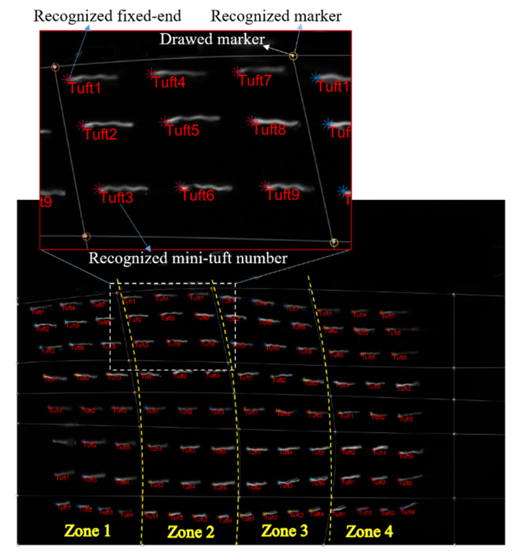
The time-averaged digital mini-tufts are calculated for analyzing the time-averaged flow behavior. For more intuitive observation of features, the mean digital mini-tufts of each group of the time-averaged digital mini-tufts are calculated. The current method proposed is realized well for the digitalization of mini-tufts.
(2)
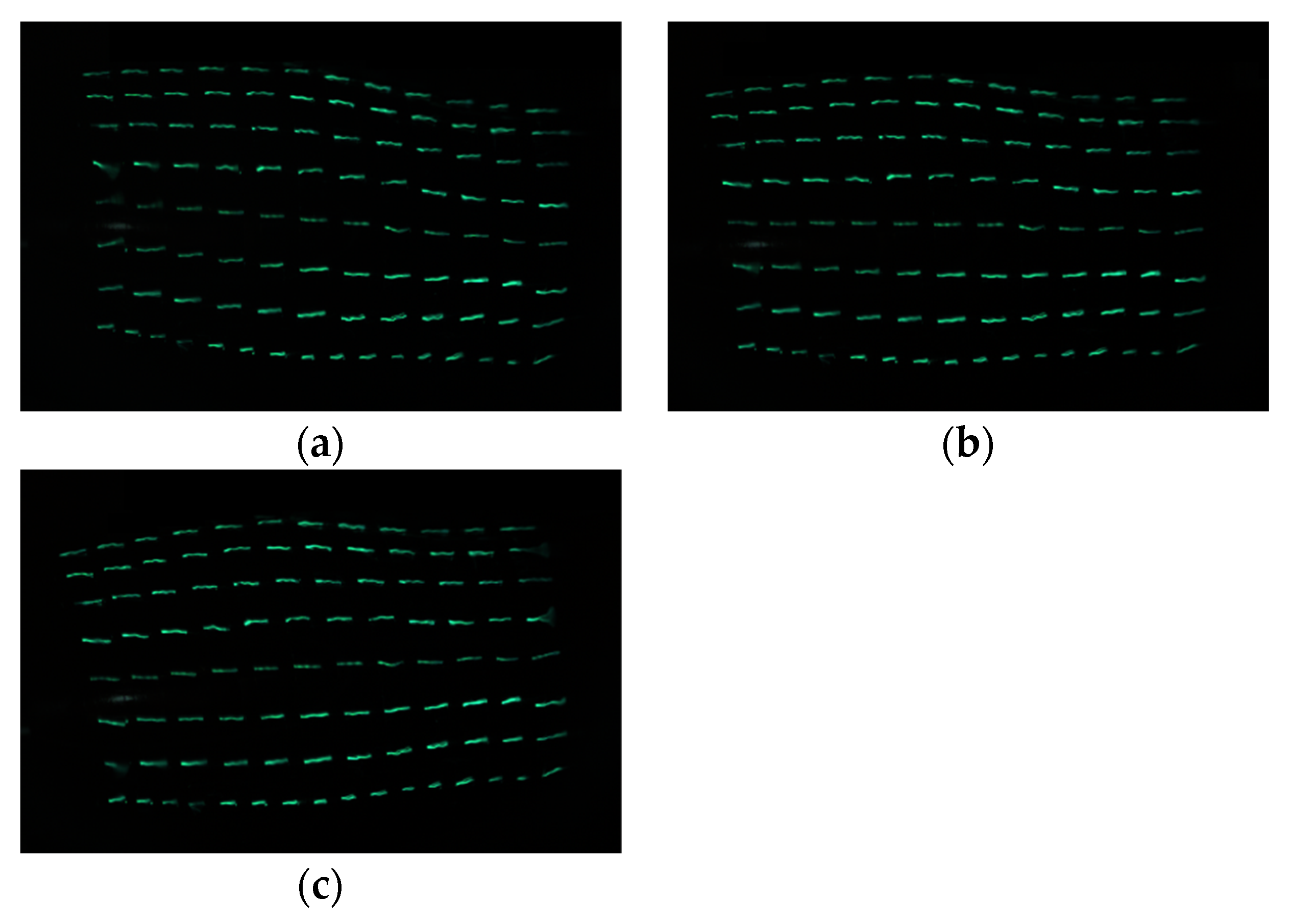
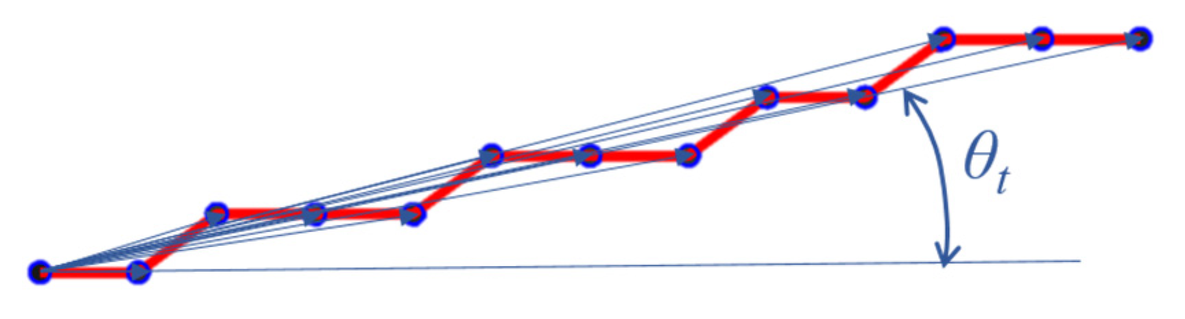
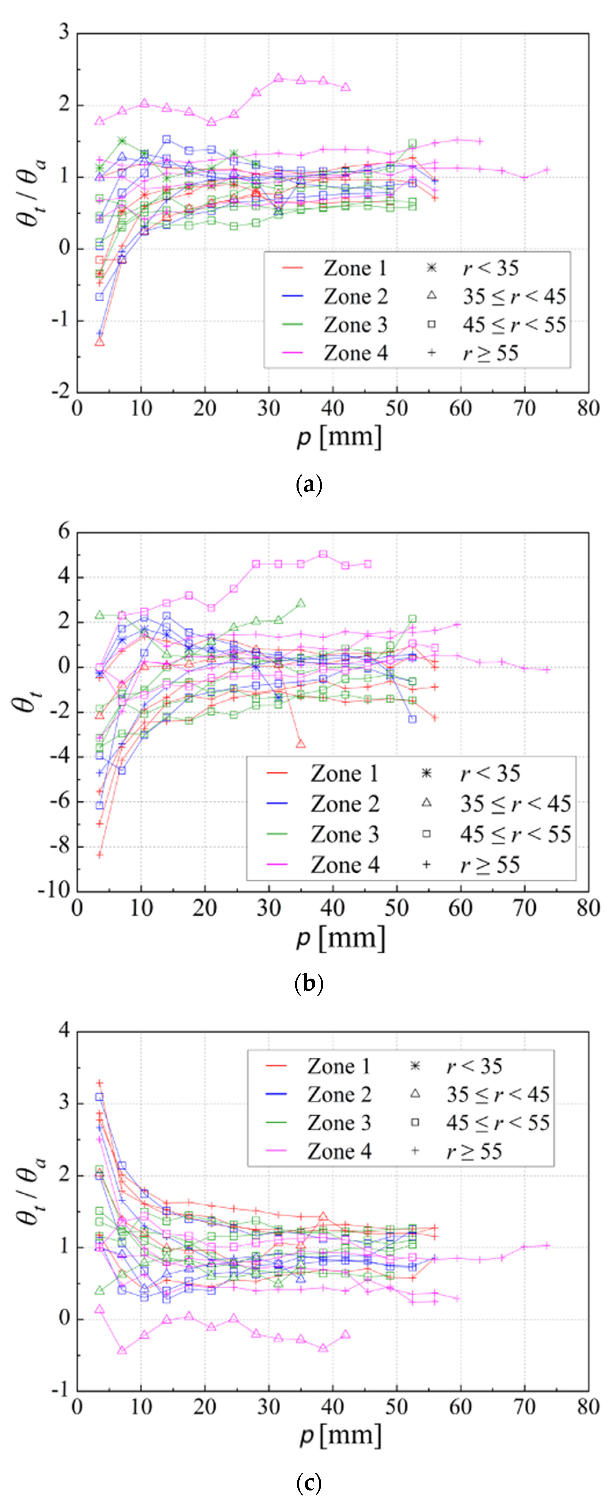
With regard to the target model in the experiment, though the angle of attack varies, the latter segment (after around 20 mm) of almost all tufts follow the inflow direction on the model surface well.
(3)
The mean tuft transient oscillation under the same flow surrounding the same model is not impacted by the angle of attack.
(4)
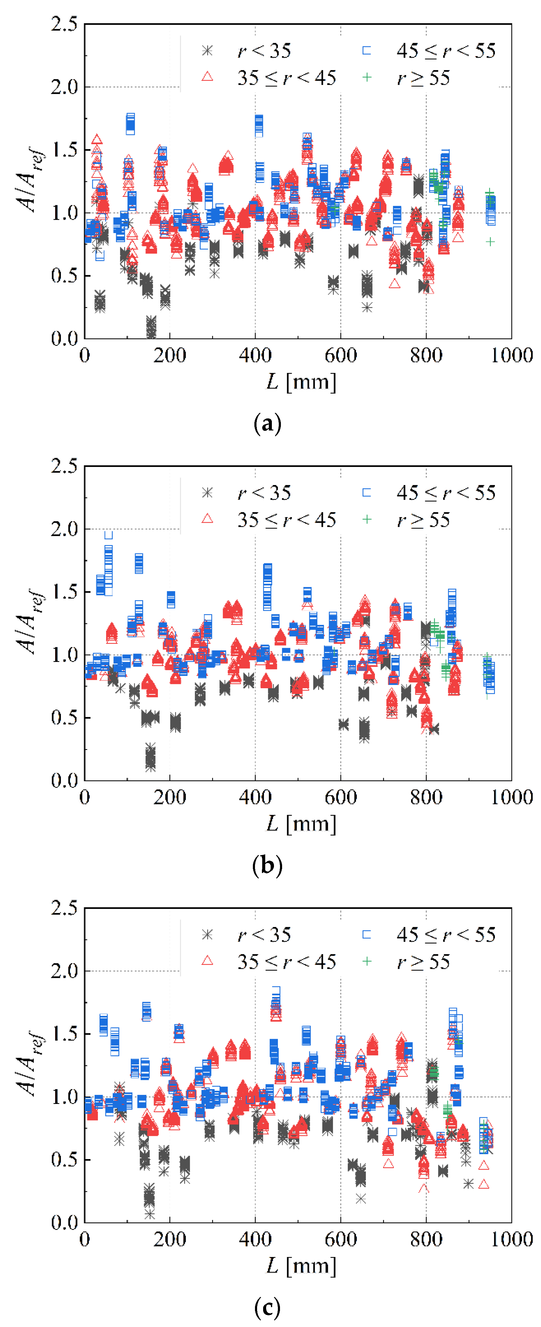
According to the mean values of A/Aref, the tufts on the middle part of the model are larger than those on the two terminals, which indicates that the transient fluid is oscillating more intensively on the middle part of the irregularity cylinder than on the two terminals of the model.

Author Contributions

Conceptualization, L.C.; methodology, L.C.; software, S.M.; formal analysis, S.M.; investigation, S.M.; resources, L.C.; writing—original draft preparation, S.M. and L.C.; writing—review and editing, L.C.; supervision, L.C.; project administration, L.C.; funding acquisition, L.C. All authors have read and agreed to the published version of the manuscript.

Funding

This research was funded by the key research program of the CAS innovation academy for light-duty gas turbine (No. CXYJJ21-ZD-01), the CAS key research program of frontier sciences (No. ZDBS-LY-JSC018), and the CAS start-up Program.

Data Availability Statement

The data that support the findings of this study are available within the article.

Acknowledgments

The authors would like to acknowledge the useful discussion with Guoshuai Li from the China Aerodynamic Research and Development Center and with Haisheng Chen from Institute of Engineering Thermophysics, Chinese Academy of Sciences, China.

Conflicts of Interest

The authors declare no conflict of interest. The funders had no role in the design of the study; in the collection, analyses, or interpretation of data; in the writing of the manuscript; or in the decision to publish the results.

References

  1. Chen, L.; Suzuki, T.; Nonomura, T.; Asai, K. Flow visualization and transient behavior analysis of luminescent mini-tufts after a backward-facing step. Flow Meas. Instrum. 2019, 71, 101657. [Google Scholar] [CrossRef]
  2. Nakayama, Y. Chapter 16—Flow visualization. In Introduction to Fluid Mechanics, 2nd ed.; Nakayama, Y., Ed.; Elsevier: London, UK, 2018. [Google Scholar]
  3. Stinebring, D.R.; Treaster, A.L. The Use of Fluorescent Mini-Tufts for Hydrodynamic Flow Visualization; Technical Memorandum No. TM-80-07; NAVY Department, The Pennsylvania State University: University Park, PA, USA, 1980. [Google Scholar]
  4. Foughner, J.T.; Hunter, W.W. Flow Visualization and Laser Velocimetry for Wind Tunnels; NASA Conference Publication: Hampton, VA, USA, 1982.
  5. Ramamurthi, K.; Tharakan, T.J. Flow visualisation experiments on free draining of a rotating column of liquid using nets and tufts. Exp. Fluids 1996, 21, 139–142. [Google Scholar] [CrossRef]
  6. Nakajima, R.; Numata, D.; Asai, K. A new approach to surface-flow visualization using fluorescence minitufts. In Proceedings of the 16th International Symposium on Flow Visualization, Okinawa, Japan, 24–27 June 2014. [Google Scholar]
  7. Mosharov, V.E. Luminescent methods for investigating surface gas flows (Review). Instrum. Exp. Tech. 2009, 52, 1–12. [Google Scholar] [CrossRef]
  8. Wieser, D.; Bonitz, S.; Lofdahl, L.; Broniewicz, A.; Nayeri, C.; Paschereit, C.; Larsson, L. Surface flow visualization on a full-scale passenger car with quantitative tuft image processing. In Proceedings of the SAE 2016 World Congress and Exhibition, Detroit, MI, USA, 12–14 April 2016. [Google Scholar]
  9. Wieser, D.; Bonitz, S.; Nayeri, C.N.; Paschereit, C.O.; Broniewicz, A.; Larsson, L.; Löfdahl, L. Quantitative Tuft Flow Visualization on the Volvo S60 under realistic driving Conditions. In Proceedings of the 54th AIAA Aerospace Sciences Meeting, AIAA SciTech, San Diego, CA, USA, 4–8 January 2016. [Google Scholar]
  10. Swytink-Binnema, N.; Johnson, D.A. Digital tuft analysis of stall on operational wind turbines. Wind. Energy 2016, 19, 703–715. [Google Scholar] [CrossRef]
  11. Hui, Z.; Hou, J.; Deng, L. Key technologies study of fluorescent mini-tuft application in the low-speed wind tunnel tests. J. Exp. Fluid Mech. 2015, 29, 92–96. [Google Scholar]
  12. Wang, Z. Some New Applications of the fluorescent mini tuft technique. In Flow Visualization VI; Tanida, Y., Miyashiro, H., Eds.; Springer: Berlin/Heidelberg, Germany, 1992. [Google Scholar]
  13. Htun, Y.E.; Myint, Z.Y.M. Some principles of flow visualization techniques in wind tunnels. In Proceedings of the 82nd IIER International Conference, Berlin, Germany, 3–4 October 2016. [Google Scholar]
  14. Stedman, D.H.; Carignan, G.R. Flow Visualization III; Hemisphere Publishing: Washington, DC, USA, 1983. [Google Scholar]
  15. Settles, G.S. Modern developments in flow visualization. AIAA J. 1986, 24, 1313–1323. [Google Scholar] [CrossRef]
  16. Nasutia, F. Flow Visualization; Academic Press: New York, NY, USA, 1974. [Google Scholar]
  17. Asanuma, T. Flow Visualization; Hemisphere Publishing Co.: Tokyo, Japan, 1977. [Google Scholar]
  18. Ristic, S. Optical methods in wind tunnel flow visualization. FME Trans. 2007, 34, 7–13. [Google Scholar]
  19. Corlett, W.A. Operational Flow Visualization Technique in the Langley Unitary Plan Wind Tunnel; NASA Conference Publication: Hampton, VA, USA, 1993; p. 2243.
  20. Ristic, S. Flow visualization techniques in wind tunnels. Part I—Non-optical methods. Sci. Tech. Rev. 2007, 57, 39–49. [Google Scholar]
  21. Ristic, S. Flow visualization techniques in wind tunnels. Part II—Optical methods. Sci. Tech. Rev. 2007, 57, 38–49. [Google Scholar]
  22. Omata, N.; Shirayama, S. Extracting quantitative three-dimensional unsteady flow direction from tuft flow visualizations. Fluid Dyn. Res. 2017, 49, 055506. [Google Scholar] [CrossRef]
  23. Steinfurth, B.; Cura, C.; Gehring, J. Tuft deflection velocimetry: A simple method to extract quantitative flow field information. Exp Fluids 2020, 61, 146. [Google Scholar] [CrossRef]
  24. Ristic, S.; Kozic, M. Investigation of the possibility to apply the LDA method for the determination of pressure coefficients on a high speed axial pump blade model. Sci. Tech. Rev. 2001, 51, 25–36. [Google Scholar]
  25. Ristic, S.; Matic, D.; Vitic, A. Determination of aerodynamical coefficients and visualization of the flow around the axisymetrical model by experimental and numerical methods. Sci. Tech. Rev. 2005, 55, 42–49. [Google Scholar]
  26. Ristic, S.; Isakovic, J.; Sreckovic, M.; Matic, D. Comparative analysis of experimental and numerical flow visualization. FME Trans. 2006, 34, 143–149. [Google Scholar]
  27. Ocokoljica, G.; Radulovica, J. Flow visualization and aerodynamical coefficients determination for the LASTA-95 model in wind tunnel T-35. Sci. Tech. Rev. 2006, 56, 63–69. [Google Scholar]
  28. Vey, S.; Lang, H.M.; Nayeri, C.N.; Paschereit, C.O.; Pechlivanoglou, G. Extracting quantitative data from tuft flow visualizations on utility scale wind turbines. J. Phys. Conf. Ser. 2014, 524, 012011. [Google Scholar] [CrossRef]
  29. Bonitz, S.; Wieser, D.; Broniewicz, A.; Larsson, L.; Lofdahl, L.; Nayeri, C.N.; Paschereit, C. Experimental investigation of the near wall flow downstream of a passenger car wheel arch. SAE Int. J. Passenger Cars Mech. Syst. 2018, 11, 22–34. [Google Scholar] [CrossRef]
  30. Chen, L.; Suzuki, T.; Nonomura, T.; Asai, K. Characterization of luminescent mini-tufts in quantitative flow visualization experiments: Surface flow analysis and modelization. Exp. Therm. Fluid Sci. 2019, 103, 406–417. [Google Scholar] [CrossRef]
Figure 1. Experimental set-up: model with luminescent mini-tufts and photography device, Reprinted with permission from Ref. [30]. 2019, Elsevier.
Aerospace 09 00507 g001
Figure 2. Experimental model.
Aerospace 09 00507 g002
Figure 3. Snapshot example. (a) θa = 4°; (b) θa = 0°; (c) θa = −4°.
Aerospace 09 00507 g003
Figure 4. The process flow of luminescent mini-tufts recognition.
Aerospace 09 00507 g004
Figure 5. Single mini-tuft recognition example.
Aerospace 09 00507 g005
Figure 6. Angle of luminescent mini-tuft.
Aerospace 09 00507 g006
Figure 7. Recognized mean mini-tufts classification.
Aerospace 09 00507 g007
Figure 8. Mean luminescent mini-tuft angle varies on different positions of tuft. (a) θa = 4°; (b) θa = 0°; (c) θa = −4°.
Aerospace 09 00507 g008
Figure 9. Transient oscillation of luminescent mini-tuft variations with their transversal position on the model (r’s unit is mm). (a) θa = 4°; (b) θa = 0°; (c) θa = −4°.
Aerospace 09 00507 g009
Table 1. Mean values of A/Aref with different tuft lengths.
Tuft Lengthθa = 4°θa = 0°θa = −4°
r < 350.650.670.69
35 ≤ r < 451.120.970.98
45 ≤ r < 551.101.131.12
r ≥ 551.171.061.00
Table 2. Mean and square deviation of A/Aref of different zones of model with θa = 4°.
Zone NumberMeanSquare Deviation
10.890.23
21.020.17
31.020.20
40.960.22
Table 3. Mean and square deviation of A/Aref of different zones of model with θa = 0°.
Zone NumberMeanSquare Deviation
10.970.25
21.030.16
30.990.19
40.910.22
Table 4. Mean and square deviation of A/Aref of different zones of model with θa = −4°.
Zone NumberMeanSquare Deviation
10.960.22
21.040.17
30.990.20
40.920.28
Publisher’s Note: MDPI stays neutral with regard to jurisdictional claims in published maps and institutional affiliations.

