Distributed Conflict Resolution at High Traffic Densities with Reinforcement Learning

Abstract

Future operations involving drones are expected to result in traffic densities that are orders of magnitude higher than any observed in manned aviation. Current geometric conflict resolution (CR) methods have proven to be very efficient at relatively moderate densities. However, at higher densities, performance is hindered by the unpredictable emergent behaviour from neighbouring aircraft. Reinforcement learning (RL) techniques are often capable of identifying emerging patterns through training in the environment. Although some work has started introducing RL to resolve conflicts and ensure separation between aircraft, it is not clear how to employ these methods with a higher number of aircraft, and whether these can compare to or even surpass the performance of current CR geometric methods. In this work, we employ an RL method for distributed conflict resolution; the method is completely responsible for guaranteeing minimum separation of all aircraft during operation. Two different action formulations are tested: (1) where the RL method controls heading, and speed variation; (2) where the RL method controls heading, speed, and altitude variation. The final safety values are directly compared to a state-of-the-art distributed CR algorithm, the Modified Voltage Potential (MVP) method. Although, overall, the RL method is not as efficient as MVP in reducing the total number of losses of minimum separation, its actions help identify favourable patterns to avoid conflicts. The RL method has a more preventive behaviour, defending in advance against nearby neighbouring aircraft not yet in conflict, and head-on conflicts while intruders are still far away.

1. Introduction

Should predictions become reality, the aviation field will have to prepare for the introduction of a large number of mass-market drones. It is estimated that as many as 400,000 drones will provide services in European airspace by 2050 [1]. At least 150,000 are expected to operate in an urban environment for multiple delivery purposes. This is expected to result in traffic densities that are orders of magnitude higher than any observed in manned aviation. As a result, automation of separation assurance in unmanned aviation is a priority, as drones must be capable of conflict detection and resolution (CD&R) without human intervention. Both the FAA [2] and the ICAO [3] have ruled that a UAS must have Sense and Avoid capability in order to be allowed in civil airspace.

Operations with high traffic densities also increase the likelihood of aircraft encountering so called ‘multi-actor’ conflict situations. These are situations where an aircraft is in a state of conflict with multiple other aircraft at the same time. In a pairwise conflict, conflict resolution (CR) methods, or rules, can be implemented so that aircraft work together towards preventing a loss of minimum separation (i.e., implicit coordination). However, these rules alone cannot predict the traffic patterns that emerge from successive conflict avoidance manoeuvres and consequent knock-on effects. As a result, these methods can no longer predict which characteristics lead to optimal behaviour at these higher densities.

Through continuous improvement, reinforcement learning (RL) can potentially identify trends and patterns in this otherwise unpredictable emergent behaviour. RL can adjust to this emergent behaviour, and develop a large set of rules and weights for different conflict geometries, from the knowledge of the environment captured during training. In this specific context, a high traffic operating scenario is essentially a multi-agent problem, with emergent behaviour and complexity arising as a result of aircraft interacting. The knowledge gathered from the actions performed by RL methods to increase safety, can be used to both improve current conflict resolution methods and support the decision-making process of air traffic controllers.

In this work, we pose the following questions:

• Can RL methods, by adapting to the global patterns emerging from multi-actor conflicts and knock-on effects, find geometry-specific resolution manoeuvres capable of improving safety compared to current geometric CR methods?
• Is it possible to derive conflict resolution rules, from the actions performed by the RL method, that improve the performance of current geometric CR methods?

The answer to these questions must take into account the limitations of reinforcement learning approaches. The complexity of training, and consequently the time required for the method to reach an optimal performance, is directly proportional to the number of state-action combinations. Consequently, environments are often discretised to a level such that only a small amount of information is available to the RL method. Additionally, to reach an optimal solution within an acceptable amount of time, degrees of freedom are often limited, as exemplified in previous work such as Pham [4]. Finally, aircraft must prioritize global safety as well as their own. Global safety can only be achieved through coordinated actions. Nevertheless, any level of coordination between agents is non-trivial. A common approach to incite coordination is to resort to multi-agent RL, as exemplified by Isufaj [5]. However, this limits the number of aircraft, as the RL method must learn different policies per aircraft. In summary, it may be that the limitations set in an RL method, to limit its convergence time, may also limit its ability to generalise towards unseen conflict geometries and/or traffic densities. The result would be an RL method with limited rules/solutions, which represents the main issue with geometric CR methods.

In this work, an operational unmanned airspace scenario is implemented with the open-source, multi-agent ATC simulation tool BlueSky [6]. We use the Soft Actor–Critic (SAC) algorithm, as created by UC Berkely [7], for the RL method responsible for conflict resolution. Several versions of the method are tested in order to determine the best action formulation: (1) action and speed variation only; and (2) action, speed, and altitude variation. Additionally, we consider all aircraft homogeneous and test whether a global safety reward can lead to coordinated movements. The final efficacy and efficiency of the RL method are directly compared to a state-of-the-art geometric distributed CR algorithm, the Modified Voltage Potential (MVP) [8], which resolves conflicts with a minimum path deviation. Finally, rules that can be used to improve the behaviour of current geometric CR methods are derived from the actions performed by the RL method.

2. Conflict Resolution with Reinforcement Learning Method

This section defines the parameters of the RL method responsible for conflict resolution, which guarantees minimum separation between all aircraft. When applying RL to mitigate undesirable emergent patterns resulting from multi-actor conflicts and knock-on effects, several questions follow:

• What information does the RL method need to successfully resolve conflicts?
• Which degrees of freedom should the RL method control to perform effective conflict resolution manoeuvres?

Additionally, two problems arise when using RL in cooperative multi-aircraft situations. First, with each action, the next state depends not only on the action performed by the ownship, but on the combination of that action with the actions simultaneously performed by the neighbouring aircraft. From the point of view of each agent, the environment is non-stationary and, as training progresses, modifies in a way that cannot be explained by the agent’s behaviour alone. Second, a certain action may be favourable to the ownship but may have negative results on the neighbouring aircraft. The latter may, for example, have to perform bigger deviations from their nominal path to avoid a loss of minimum separation with the ownship. In the following subsections, the parameters chosen to tackle these challenges will be discussed.

Note that, with the aim of answering the second question (i.e., which degrees of freedom the RL method should control), two different action formulations will be tested and directly compared. For the larger action formulation (i.e, with altitude variation on top of heading, and speed variation), extra information is also added to the state formulation, so that the method knows which values to employ for the altitude variation.

Table 1. Action formulation for RL method. First, the RL method will be tested controlling only heading and speed variation. Second, it will also control vertical speed variation on top of the former elements.

Action	Limits	Units	Dimension
Heading Variation	[−1,+1] transforms to [−15,+15]	${}^{\circ }$	1
Speed Variation	[−1,+1] transforms to [−5,+5]	m/s	1
Vertical Speed Variation	[−1,+1] transforms to [−2,+2]	m/s	1

and

Table 2. State formulation for RL method. Note that the current altitude and relative altitude to aircraft, both in grey, are only added to the state formulation when the RL method controls altitude on top of heading and speed variation.

Element	Dimension
Current heading	1
Relative bearing to target	1
Current speed	1
Current altitude	1
Current distance to #NEIGHBOURS	#NEIGHBOURS
Distance at CPA with #NEIGHBOURS	#NEIGHBOURS
Time to CPA with #NEIGHBOURS	#NEIGHBOURS
Relative heading to #NEIGHBOURS	#NEIGHBOURS
Relative altitude to #NEIGHBOURS	#NEIGHBOURS

identify the parameters in the state and action formulations, respectively. The elements used only when altitude variation is possible, are highlighted in grey.

2.1. Agent

We employ an RL agent responsible for guaranteeing a minimum separation distance between the aircraft at all times. This agent may be considered to have centralized learning with a distributed policy. The RL method performs actions based on the information specific to each aircraft, namely its current state, distance, and relative heading to the nearest neighbours (decentralized execution). However, during training, rewards are based on centralised information, i.e., the global number of losses suffered by all aircraft in the environment (centralized learning).

2.2. Learning Algorithm

An RL method consists of an agent interacting with an environment in discrete timesteps. At each timestep, the agent receives the current state of the environment and performs an action in accordance, for which it receives a reward. An agent’s behavior is defined by a policy which maps states to actions. The goal is to learn a policy which maximizes the expected cumulative reward over time. Defining the reward is one of biggest problems affecting the performance of RL methods. The reward tells the agent what to do, not how to do it [9]. Nevertheless, the agent should complete the task in the most desirable manner. However, it can be that it finds undesirable ways to satisfy the objective, even if the algorithm was implemented flawlessly. Finally, the defined reward also influences convergence speed, and the likelihood of the agent becoming stuck in local optima.

In this work, we use the Soft Actor–Critic (SAC) as defined in [7]. SAC is an off-policy actor–critic deep RL algorithm. It employs two different deep neural networks to approximate an action-value function and a state-value function. The Actor maps the current state based on the action that it estimates to be optimal, while the Critic evaluates the action by calculating the value function. The main feature of SAC is its maximum entropy framework: the actor aims to maximize the expected reward while also maximizing entropy. This results in an exploration/exploitation trade-off. The agent is explicitly pushed towards the exploration of new policies while at the same time avoiding being stuck in sub-optimal behaviour.

2.3. Action Formulation

The RL agent determines the action to be performed for the current state. The incoming state values are transformed through each layer of the neural network, in accordance to the neurons’ weights and the activation function in each layer. The activation function takes as input the output values from the previous layer and converts them into a form that can be taken as input to the next layer. The output of the final layer must be turned into values that can be used to define the elements of the state of the aircraft that the RL agent controls. In this study, all actions are computed using a tanh activation function. The tanh function outputs values between −1 and +1, which can prevent the output value of the policy network from being too large and causing great state changes per action [10].

The output of the tanh function is translated to a variation of the current state of the ownship, as identified in Table 1. Note that a variation in heading of $-{15}^{\circ }$ and $+{15}^{\circ }$ indicates a turn of ${15}^{\circ }$ to the left and ${15}^{\circ }$ to the right, respectively. With regard to speed, the ownship can reduce or increase its speed up to 5 m/s every timestep. A timestep of 1 s is employed. Finally, the vertical speed can decrease or increase every action to a maximum of 2 m/s. These values were empirically tuned. Different values may be used depending on the operational environment. However, the following should be taken into account:

• A greater range of state variation increases the number of different aircraft states that the RL agent may set with each action. Thus, also increasing the amount of possible actions and, in turn, convergence time. Additionally, small variations in the agent’s actions will have a greater impact on the aircraft’s state. This requires the agent to learn a high level of precision.
• Considering the acceleration limits of the aircraft models involved. At each timestep, there is a maximum state variation that an aircraft may achieve. With great state variations, the reward received by the RL method may not be based on the state output by the method. Instead, it will be a result of the maximum variation that the aircraft was able to achieve within the available time. This may make it harder for the RL method to correctly relate actions to expected rewards.

Two different action formulations are tested: (1) the RL method controls heading, and speed variation; or (2) heading, speed, and altitude variation. The two action formulations allow for defining what the best usage of the RL method is. On the one hand, increasing the size of the action formulation may decrease optimality of the actions performed by the RL method. The latter must pick from a much larger set of state-action combinations. However, the RL method also has more control over aircraft and thus may influence the environment to a greater extent.

2.4. State Formulation

The state input into the RL method must contain the necessary data for the RL agent to successfully resolve conflicts. Such a decision requires information regarding the current state of the ownship, and the relative position and speed of the neighbouring aircraft. However, representing all aircraft in the airspace is impractical. We limit the state information to the closest aircraft, in terms of physical distance. We consider the closest four aircraft. This decision is a balance between giving enough information to the method, so it can make a based decision, while keeping the state formulation to a minimum size. The size of the problem’s solution grows exponentially with the number of possible state permutations. The size of the state formulation must thus be limited to guarantee that the method trains within an acceptable amount of time. However, it may be that considering only the four closest aircraft is not ideal for every operational scenario; such must be decided on a case-by-case basis.

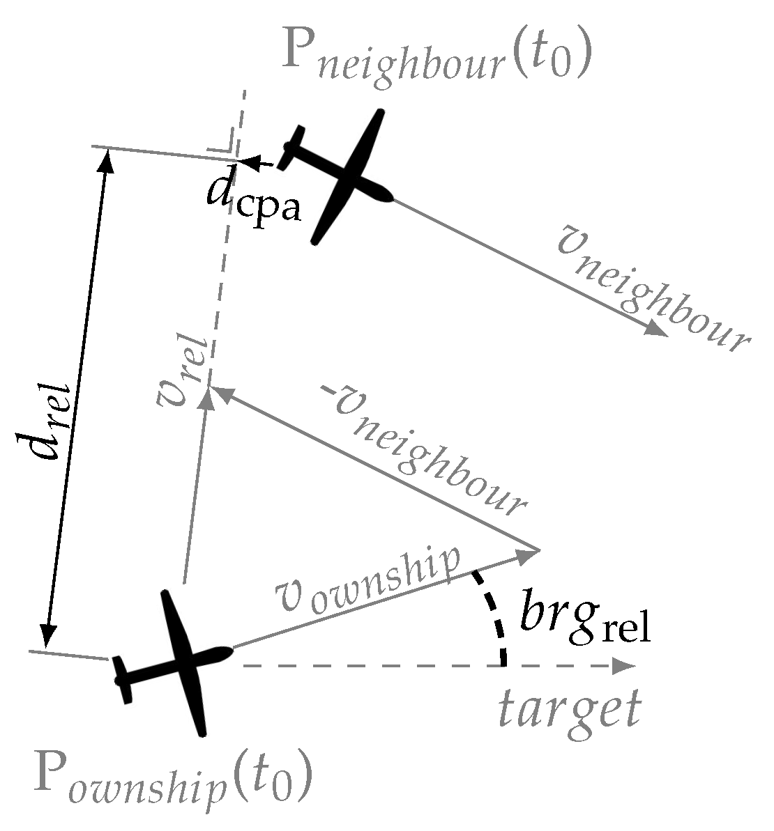
As defined in Table 2, the RL method is informed of the ownship’s current heading, bearing to target, and current speed. Regarding neighbouring aircraft, it has knowledge on their current distance to the ownship, relative heading, distance at the closest point of approach (CPA), and time to CPA. Figure 1 depicts the data used to defined the relation between ownship and neighbouring aircraft in the horizontal plane. When the agent also controls altitude variation, it additionally receives information on the ownship’s current altitude and relative altitude to the closest aircraft.

2.5. Reward Formulation

The reward given to the RL agent is primarily based on safety. However, within safety, several factors may be considered. The paramount objective is to lead the agent to favour deconflicting actions that reduce the likelihood for LoSs. Thus, the reward is set based on the number of LoSs. Moreover, to favour coordinated manoeuvres which improve global safety, the reward given for each action is based on the number of LoSs suffered by all aircraft in the previous time step. A value of $-1$ is added to the reward for every LoS that occurred in the environment since the action was initiated, i.e., in the last timestep. A negative factor of this reward approach is that the reward to an action will be affected by unrelated LoSs, suffered by other (far away) aircraft. Such may increase convergence time, or even affect the capacity of the RL method to converge towards optimal values. The consequences of this reward implementation will be further examined in the discussion of the results.

3. Experiment: Conflict Resolution with Reinforcement Learning

The following subsections define the properties of the performed experiment. The latter aims at using RL to perform optimal deconflicting manoeuvres at high traffic densities. Note that the experiment involves a training and a testing phase. First, the RL method is trained continuously with a set of 16 known traffic scenarios. For reference, without conflict resolution, each training episode has on average about 1000 conflicts in 20 min running time. The evolution of the amount of LoSs and conflicts, for every training episode, is directly compared with the average total number of LoSs and conflicts when running these 16 scenarios with the MVP. Additionally, the final optimal actions of the RL method for every conflict situation are directly compared with the ones that MVP would perform for those exact situations. Each training scenario runs for 20 min. Second, the RL method is tested with unknown traffic scenarios at the same and different traffic densities that it was trained in. In this case, the safety, stability, and efficiency results of the method are directly compared to running the same scenarios with the MVP method. Each testing scenario runs for 30 min.

3.1. Flight Routes

The measurement area is square-shaped with an area of 144 NM². The aircraft spawn locations (origins) are placed on the edges of this area, with a minimum spacing equal to the minimum separation distance, to avoid conflicts between recently spawned aircraft and aircraft arriving at their destination. All aircraft fly a straight route towards their destination, at the same altitude level. Three waypoints are added between origin and target points which aircraft must pass through in order. Ideally, aircraft would only operate within the measurement area, thereby ensuring a constant density of aircraft within that area. However, aircraft may temporarily leave the measurement area during the resolution of a conflict and should not be deleted in this case. Therefore, a second, larger area encompassing the measurement area is considered: the experiment area. As a result, aircraft in a conflict situation close to their origin or destination are not deleted incorrectly from the simulation. Ultimately, an aircraft is removed from the simulation once it leaves the experiment area. We assume a no-boundary setting, with sufficient flight space around the measurement area, in order to avoid edge effects from influencing the results.

3.2. Apparatus and Aircraft Model

The open air traffic simulator BlueSky [6] is used in order to test the efficiency of RL in resolving conflicts. The performance characteristics of the DJI Mavic Pro were used to simulate all vehicles. Here, speed and mass were retrieved from the manufacturer’s data, and common conservative values were assumed for turn rate (max: 15 °/s) and acceleration/breaking (1.0 kts/s).

3.3. Minimum Separation

The value of the minimum safe separation distance may depend on the density of air traffic and the region of the airspace. For unmanned aviation, there are no established separation distance standards yet, although 50 m for horizontal separation is a value commonly used in research [11], and will therefore be used in these experiments. For vertical separation, 15 ft was assumed.

3.4. Calculation of Closest Point of Approach (CPA)

In this work, we assume linear propagation of the current state of all aircraft involved to calculate the CPA between two aircraft. Using this approach, the time to CPA (in seconds) is calculated as:

$$t_{CPA}=-\frac{{\overrightarrow{d}}_{rel}·{\overrightarrow{v}}_{rel}}{{\overrightarrow{v}}_{rel}^2},$$

(1)

where ${\overrightarrow{d}}_{rel}$ is the Cartesian distance vector between the involved aircraft (in meters), and ${\overrightarrow{v}}_{rel}$ the vector difference between the velocity vectors of the involved aircraft (in meters per second).

The distance between aircraft at CPA (in meters) is calculated as:

$$d_{CPA}=\sqrt{{\overrightarrow{d}}_{rel}^2-{t_{CPA}}^2·{\overrightarrow{v}}_{rel}^2}.$$

(2)

Both $t_{CPA}$ and $d_{CPA}$ are added to the state formulation of the RL method as previously defined in Table 2.

3.5. Conflict Resolution (Modified Voltage Potential Only)

As previously mentioned, the results obtained with the RL method will be directly compared to those obtained with the state-of-the-art CR method MVP. We employ the method as defined by Hoekstra [8,12]. An important difference between the RL method and MVP, from the very beginning, is how they select ‘intruders’. We apply as little bias on the state formulation of the RL method as possible. Thus, we simply select aircraft based on their distance to the ownship. It may be considered that adding only the aircraft that the ownship is in conflict with might be more efficient. However, the RL method would then not have a full perception of the consequence of its actions when moving towards a non-conflicting nearby aircraft.

MVP, on the other hand, considers only aircraft that are actually in conflict in its resolution. Conflicts are detected when $d_{CPA}<R_{PZ}$, and $t_{in}\le t_{lookahead}$, where $R_{PZ}$ is the radius of the protected zone (PZ), or the minimum horizontal separation, and $t_{lookahead}$ is the specified look-ahead time. A look-ahead time of 300 s is used for conflict detection and resolution. This value was selected since, empirically, it was found to result in the best behaviour of the MVP method in this specific simulation environment. Note that this is a larger look-ahead time than typically used in unmanned aviation, where values can be even less than 1 min. Nevertheless, these values are often considered in constrained airspace, as larger look-ahead times would result in the inclusion of false conflicts past the borders of the environment [13]. Moreover, it is likely this large look-ahead time would perform worse in environments with uncertainty regarding intruders’ current position and future path. Additionally, delays in data transmission and severe meteorologic conditions are often a source of errors in the estimation of future positions.

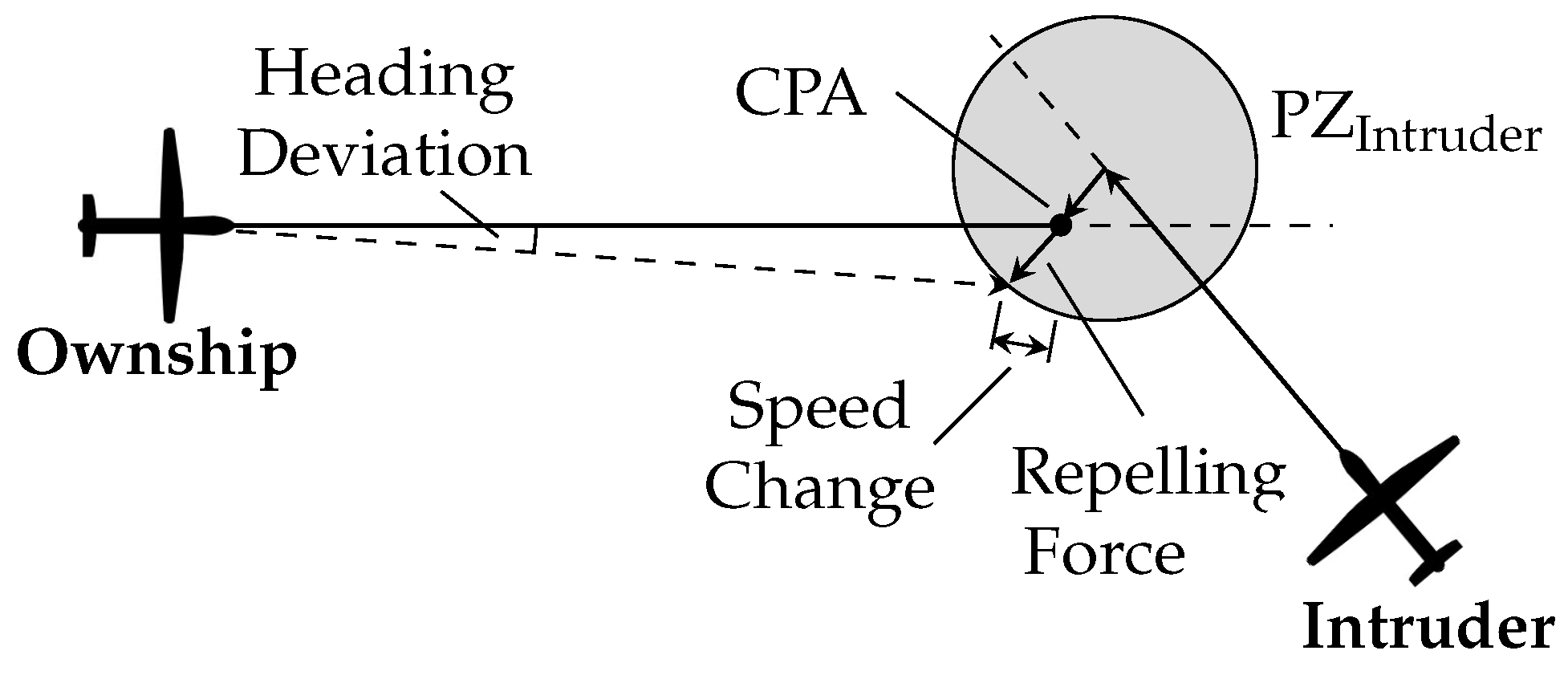
The behaviour of MVP is displayed in Figure 2. MVP uses the predicted future positions of both ownship and intruder CPA. These calculated positions “repel” each other, and this “repelling force” is converted to a displacement of the predicted position at CPA. The avoidance vector is calculated as the vector starting at the future position of the ownship and ending at the edge of the intruder’s protected zone, in the direction of the minimum distance vector. This displacement is thus the shortest way out of the intruder’s protected zone. Dividing the avoidance vector by the time left to CPA, yields a new speed, which can be added to the ownship’s current speed vector resulting in a new advised speed vector. From the latter, a new advised heading and speed can be retrieved. The same principle is used in the vertical situation, resulting in an advised vertical speed. In a multi-conflict situation, the final avoidance vector is determined by summing the avoidance vectors from all intruders. By taking the shortest way out, each aircraft in a conflict will take (opposite) measures to evade the other in a way that makes MVP implicitly coordinated.

3.6. Independent Variables

The main independent variable is the method used to resolve conflicts and assure minimum separation between all aircraft; this is either the RL or the MVP method. Both the training and testing results of the RL method are directly compared to the results obtained when the same traffic scenarios are run with the MVP method instead. Additionally, different action formulations are employed in order to analyse how the RL method reacts to different degrees of freedom: (1) the CR method only performs heading and speed variation to resolve conflicts; (2) the CR method uses heading, speed, and altitude variation. The variations of heading, speed, and altitude performed by the RL method during training, are directly compared of the ones that the MVP would perform for the exact same conflict situations.

Finally, during testing, different traffic densities are introduced to analyse how the RL method performs at traffic densities in which it was not trained. These range from low to high as per

Table 3. Traffic volume used in the experimental simulations.

	Training (20 min Simulation)	Testing (30 min Simulation)
Traffic Density	Medium	Low	Medium	High
Number of aircraft per 10,000 NM2	40,000	20,000	40,000	60,000
Number of instantaneous aircraft	576	288	576	863
Number of spawned aircraft	886	665	1330	1994

. At high densities, vehicles spend more than 10% of their flight time avoiding conflicts [14]. The RL agent is trained at a medium traffic density, and is then tested with low, medium, and high traffic densities. In this way, it is possible to assess the efficiency of an agent performing in a traffic density different from the one in which it was trained.

3.7. Dependent Variables

Three different categories of measures are used to evaluate the effect of the different conflict resolution methods in the simulation environment: safety, stability, and efficiency.

3.7.1. Safety Analysis

Safety is defined in terms of the number and duration of conflicts and losses of minimum separation. The most important factor is a reduction in the total number of LoSs compared to a situation where no conflict resolution is performed. Additionally, LoSs are distinguished based on their severity according to how close aircraft get to each other, where a low separation severity is preferred. The latter is calculated as follows:

$$Lo{S}_{sev}=\frac{R_{PZ}-d_{CPA}}{R_{PZ}}.$$

(3)

3.7.2. Stability Analysis

Stability refers to the tendency for tactical conflict avoidance manoeuvres to create secondary conflicts. In the literature, this effect has been measured using the Domino Effect Parameter (DEP) [15]:

$$DEP=\frac{n_{cfl}^{ON}-n_{cfl}^{OFF}}{n_{cfl}^{OFF}},$$

(4)

where $n_{cfl}^{ON}$ and $n_{cfl}^{OFF}$ represent the number of conflicts with conflict resolution ON and OFF, respectively. A higher DEP value indicates a more destabilising method, which creates more conflict chain reactions.

3.7.3. Efficiency Analysis

Efficiency is evaluated in terms of the distance travelled and duration of the flight. Significantly increasing the path travelled and/or the duration of the flight is considered inefficient.

4. Experiment: Hypotheses

It is hypothesised that the RL method will be able to understand the concept of minimum separation and resolve the majority of conflicts. A direct performance comparison between the RL and MVP methods is uncertain at this point. On the one hand, the latter can perform geometric manoeuvres that guarantee conflict resolution with minimum path and state deviation. This is a level of precision that limits the creation of secondary conflicts. It is hypothesised that the RL method will likely perform greater state variations than the MVP method. On the other hand, the RL method is capable of adapting to the global patterns emerging from multi-actor conflicts, and knock-on effects from successive resolution manoeuvres. It can create a much larger set of rules and solutions for resolution of different conflict geometries. Whether this can help the RL method surpass the performance of the MVP method remains to be seen. Nevertheless, it is also hypothesised that the manoeuvres performed by the RL method can provide guidelines to improve the efficacy of the existing distributed, geometric CR algorithms.

Additionally, CR methods are normally able to resolve more conflicts as the degrees of freedom increase. It is expected that the MVP method will resolve more conflicts when it can vary altitude, heading, and speed versus a situation where it can only vary heading and speed. However, as the state formulation increases, so does the set of possible state-action combinations. This often results in longer training times, and not so optimal choices by an RL method. Thus, it is hypothesised that when the RL method only controls heading and speed, its final efficacy in resolving conflicts will be closer to that of the MVP method.

Finally, the RL method will be tested with different traffic densities. It is hypothesised that the method will be most efficient at low and medium traffic densities. The method is trained at medium traffic densities. The higher the traffic density, the more complex the conflicts’ geometries are to resolve, with each aircraft potentially facing multiple conflicts with multiple simultaneous intruders. Thus, the optimal actions learnt during training may not be sufficient to resolve conflicts with a higher number of intruders. Moreover, the state formulation contains only information regarding the four closest neighbouring aircraft. In a conflict situation with a considerably higher number of near-by aircraft, the method may not have enough information to resolve all conflicts with all these aircraft. As previously mentioned, the limitation of the state and action formulations to improve convergence times, may limit the ability of the RL method to generalize its actions to operational environments with different characteristics.

5. Experiment: Results

In the results section, a distinction is made between the training and the testing phases. The former shows the evolution of the RL method while training with a repeating cycle of 16 episodes, at medium traffic density, to investigate how well the RL method learns. In total, 300 episodes were run. During training, each episode ran for 20 min. Second, the trained RL method was then tested with different traffic scenarios at a low, medium, and high traffic density. For each traffic density, 3 repetitions were run with 3 different route scenarios, for a total of 9 different traffic scenarios. During the testing phase, each scenario ran for 30 min. Safety, stability, and efficiency results of the RL method are directly compared to the ones obtained when running the same scenarios the MVP method.

5.1. Training of the RL Agent for Conflict Resolution

This section presents the results of the training phase of the RL method. The latter is trained with a repeating cycle of 16 episodes at medium traffic density. Its results are directly compared with the average total number of conflicts and LoSs obtained with the MVP method with the same traffic scenarios. Furthermore, the actions performed by the method are examined in order to understand the conflict resolution decisions adopted.

5.1.1. Safety Analysis

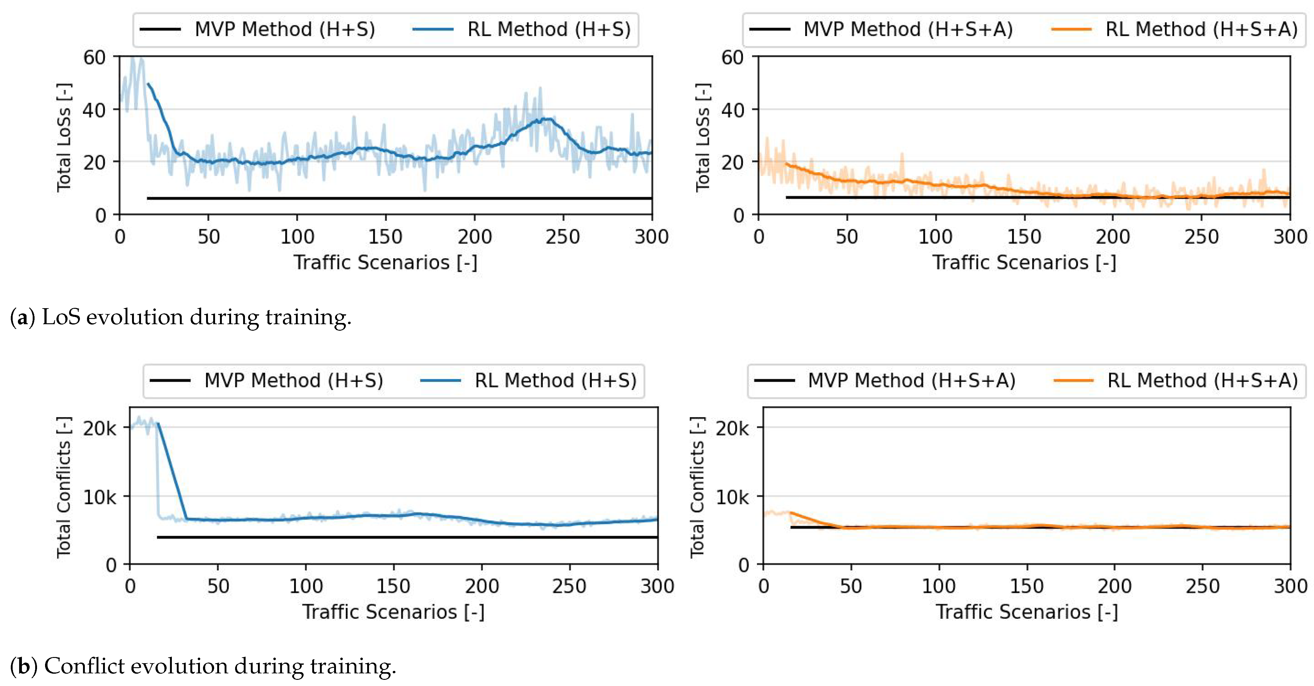
Figure 3 shows the evolution in safety performance of the RL method in terms of losses of separation (Figure 3a) and number of conflicts (Figure 3b) for both action formulations. The values obtained when both the MVP and RL methods control only the heading and speed variations are indicated by ‘MVP Method (H + S)’ and ‘RL method (H + S)’, respectively. The values with ‘(H + S + A)’ indicate the performance of the previous methods when these control altitude variation, on top of heading and speed variation. The values presented for the MVP method represent the average values for all 16 training episodes. With and without altitude deviation, the RL method is able to converge towards actions that resolve the great majority of the conflicts. Considering the total number of conflicts in Figure 3b, the RL method is able to resolve 99.7% and 99.83% of the conflicts with heading + speed and heading + speed + altitude control, respectively. Contrary to what was hypothesised, the RL method is able to achieve safety results comparable to those of the MVP when it can control more degrees of freedom. This indicates that the method is able to use the increased number of possible actions to resolve conflicts efficiently.

With only heading and speed variation, the RL method has a higher total number of LoSs than MVP. However, MVP has fewer conflicts than the RL method. Tactical CR manoeuvres typically create secondary conflicts. Deviating from the nominal path, in order to avoid conflicts, often results in a longer flight path. At high traffic densities, conflict-free airspace is scarce, and when each aircraft requires a larger portion of the airspace it often results in more conflicts. MVP employs a ‘shortest way out’ resolution strategy, limiting the space used by each aircraft, which in turn limits conflict chain reactions. The RL method resolves conflicts with path deviations larger than MVP, resulting in a higher number of secondary conflicts. The latter in turn leads to a higher final count of LoSs.

When altitude variation is also controlled, the RL method is able to reach the same level of efficacy in resolving conflicts as MVP. With the three degrees of freedom, the actions of the RL method do not have to be as precise. With all aircraft travelling at the same altitude, the success of conflict resolution may lie in having heading variations just large enough to resolve conflicts, but not so large that they move the ownship into the flight path of other aircraft. However, vertical deviation is a powerful tool that allows moving away from this one layer of traffic. As the ownship is moving to ‘free space’, it is less likely that deconflicting actions will result in secondary conflicts. Thus, such precise heading and altitude deviations are not as crucial.

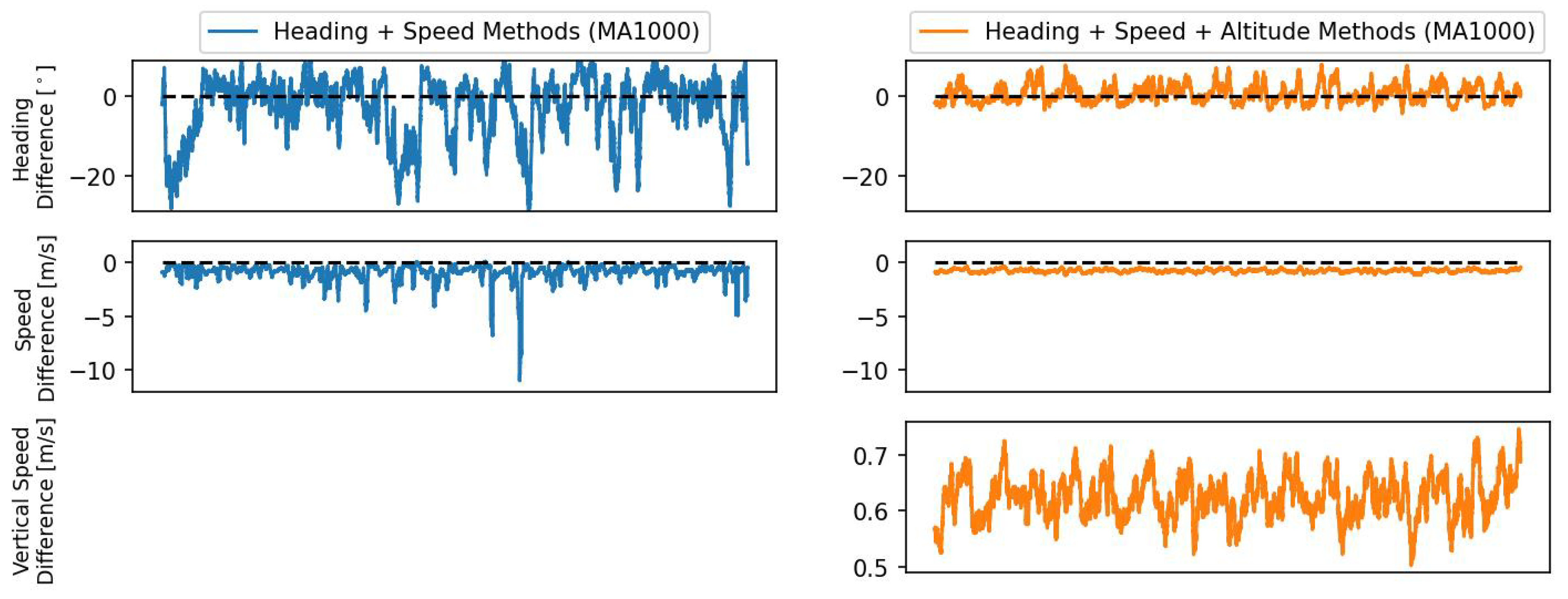
Figure 4 shows the difference in the actions carried out by the RL and MVP methods, for the same conflict situations, in all training episodes. In this case, the episodes are run with the conflict resolution decisions by the RL method. Simultaneously, the actions that MVP would output for every conflict situation are recorded, making sure that the actions can be directly compared. The graphs on the left show the difference in actions when both MVP and RL control only heading and speed variation. The top graph indicates the smallest angle difference between the heading solutions produced by the two methods. First, the difference in heading is at most 20${}^{\circ }$ between the two methods. Second, the negative values indicate that the solutions output by the MVP method are, in general, directed more towards the left than the solutions by the RL method. This may be because the RL method has a preference for resolving conflicts by turning aircraft in one direction, in this case right. This preference is not an optimal solution for every conflict geometry, but it is likely a result of the RL method finding a local optimum with this decision. These local optima are often dependent on the method’s initialisation, and a product of chance.

Regarding horizontal speed (middle graph), negative values represent a decrease in the current speed. In general, the MVP employs slightly stronger speed variations to resolve conflicts than the RL method. In comparison, the heading and speed actions produced by the RL method are much similar to those of the MVP method, when both methods can also move aircraft in the vertical dimension. It seems that, as the RL method can vary more degrees of freedom, it has learnt not to vary each degree as strongly to resolve conflicts. Finally, the RL method typically employs slightly stronger climbing actions than the MVP method.

Section 5.1.2, Section 5.1.3 and Section 5.1.4 will further explore the differences between the actions of the RL and the MVP methods.

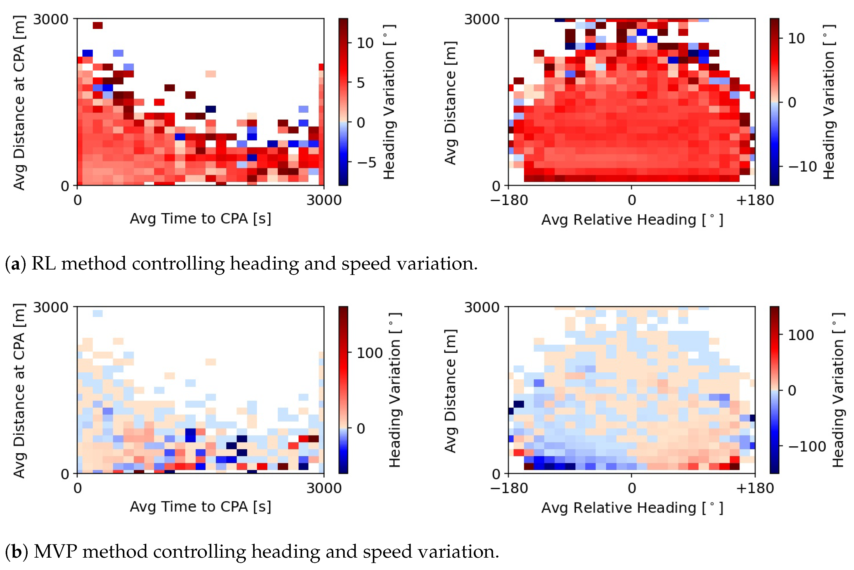
5.1.2. Heading Variation

Figure 5 connects elements in the state formulation with the average heading variation chosen by the RL and MVP methods. Interestingly, the RL method performs larger heading variations whenever the average distance at CPA or time to CPA, is smaller, but not when both are small. At every timestep, contrary to the RL method, the heading variation performed by the MVP is not limited. Thus, the extremes of the heading variation are stronger. On average, MVP performs very small heading variations, which are likely a result of the ‘shortest-way-out’ resolution strategy. However, MVP still scarcely resorts to large values. Note, however, that the great state changes output by the MVP method are likely not achievable within the observation timestep, due to performance limits. The effective state changes are likely smaller in these cases.

Considering all variables, it appears that the current distance to intruders played a bigger role in the RL method’s decisions, than the distance at CPA. The method adopts strong heading variations when neighbours are at a very short distance. This behaviour is not as consistent with a smaller distance at CPA and/or short times to CPA. Such may be because the method was able to relate negative rewards with a small distance between aircraft. Additionally, the RL method has information over the closest neighbours. These are not necessarily always the intruders with the shortest distance at CPA or time to CPA. It could be that, as a result, the method has learnt to prioritise current distance.

Additionally, as expected, the closer the intruders are, the stronger the deconflicting heading variation is. However, the RL method still resorts to strong heading deviations in some situations where the intruders are far away. Taking into account the average relative heading, these intruders would result in head-on conflicts if they were to continue with their current state. Thus, it seems as though the RL method is adopting preventive actions against possible future severe conflicts. Finally, the method shows a strong preference for turning one direction, in this case right, independently of the positions of the intruders. It may have been found that this resulted in some degree of coordination between aircraft.

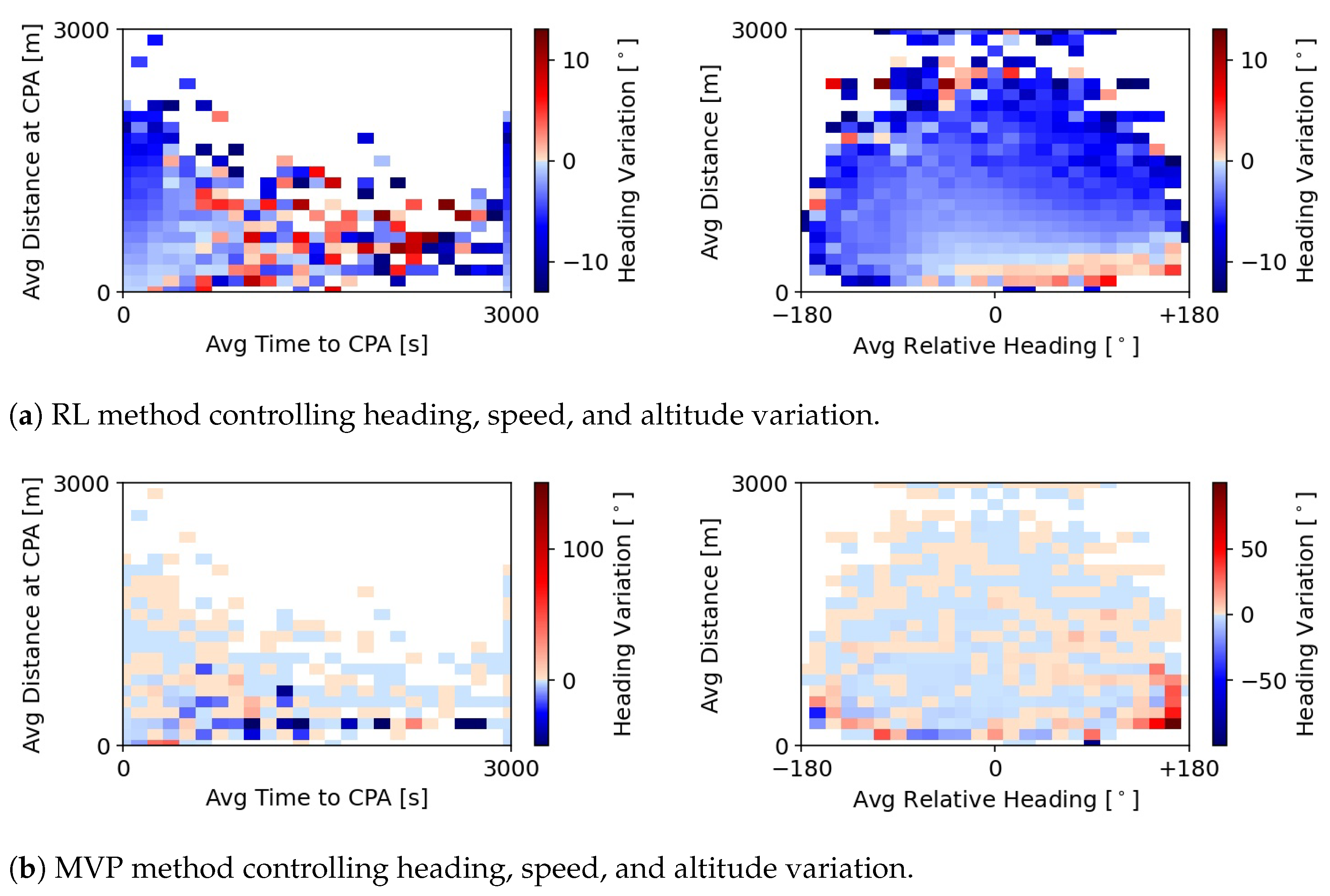
Figure 6 presents the same values as Figure 5, with the difference being that the methods can now also vary altitude. As previously seen in Figure 4, the RL method performs, on average, smaller heading variations in this case. Furthermore, here, the RL method seems to prefer heading deviations to the left. The RL method is not capable of learning when right or left might be a better option, depending on the conflict geometry. Instead, it learns that a common direction used by all aircraft results in some sort of coordination. The actions produced by the MVP are very similar to those seen in Figure 5b. This is expected; altitude variation is decoupled from heading and speed in the calculation of the resolution manoeuvre by the MVP. Thus, adding altitude variation will not alter MVP’s heading and speed deviations. However, the values in Figure 5b and Figure 6b are not exactly the same. Figure 5b shows the actions of the MVP method as it would respond to the conflict situations that occur in the traffic episodes run with the RL method that controls speed and heading variation. In comparison, Figure 6 has different conflict situations, since the episodes are run with a different RL method that now also controls altitude. Different resolution manoeuvres lead to different secondary conflict situations.

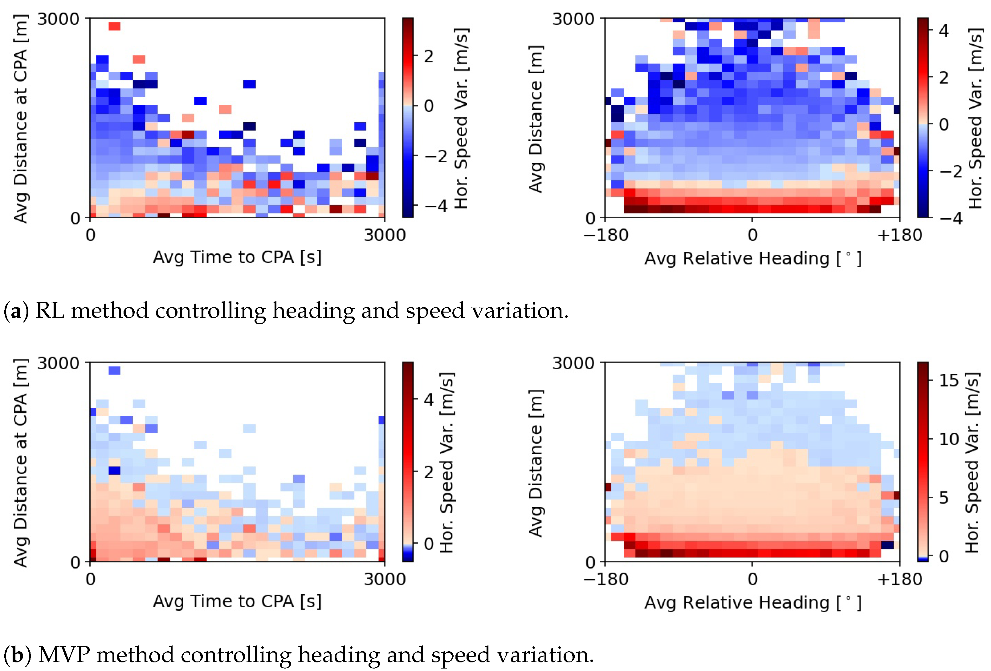
5.1.3. Speed Variation

Figure 7 shows the speed variation produced by the RL and MVP methods when these control heading and speed variation. Unlike the MVP method, the RL method often chooses to reduce speed. Such explains the higher average speed variations previously seen in Figure 4. The RL method opts for a defensive position, where speeds may be reduced in order to increase the time to CPA. Naturally, this has a negative effect on efficiency, as it increases flight time. However, efficiency is not included in the reward formulation of the method, and thus the method is not aware of this. The RL method only increases speed when neighbouring aircraft are very close in proximity, likely in an attempt to rapidly increase the distance between the ownship and these aircraft.

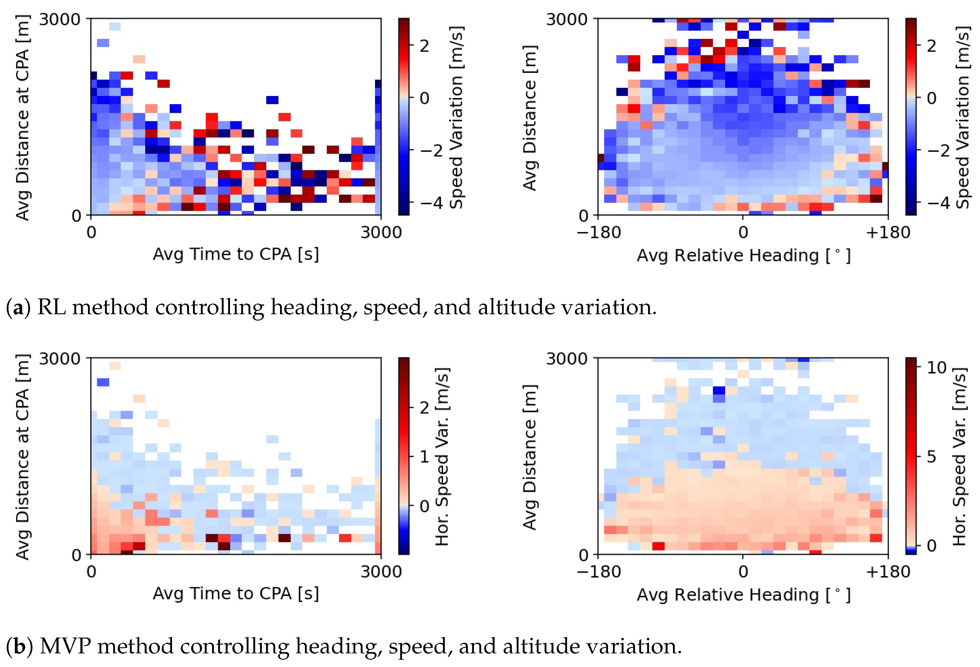
Finally, Figure 8 shows the speed variation performed by the RL method as well as MVP when these control heading, speed, and altitude variation. When the RL method also controls altitude, it outputs smaller horizontal speed variations.

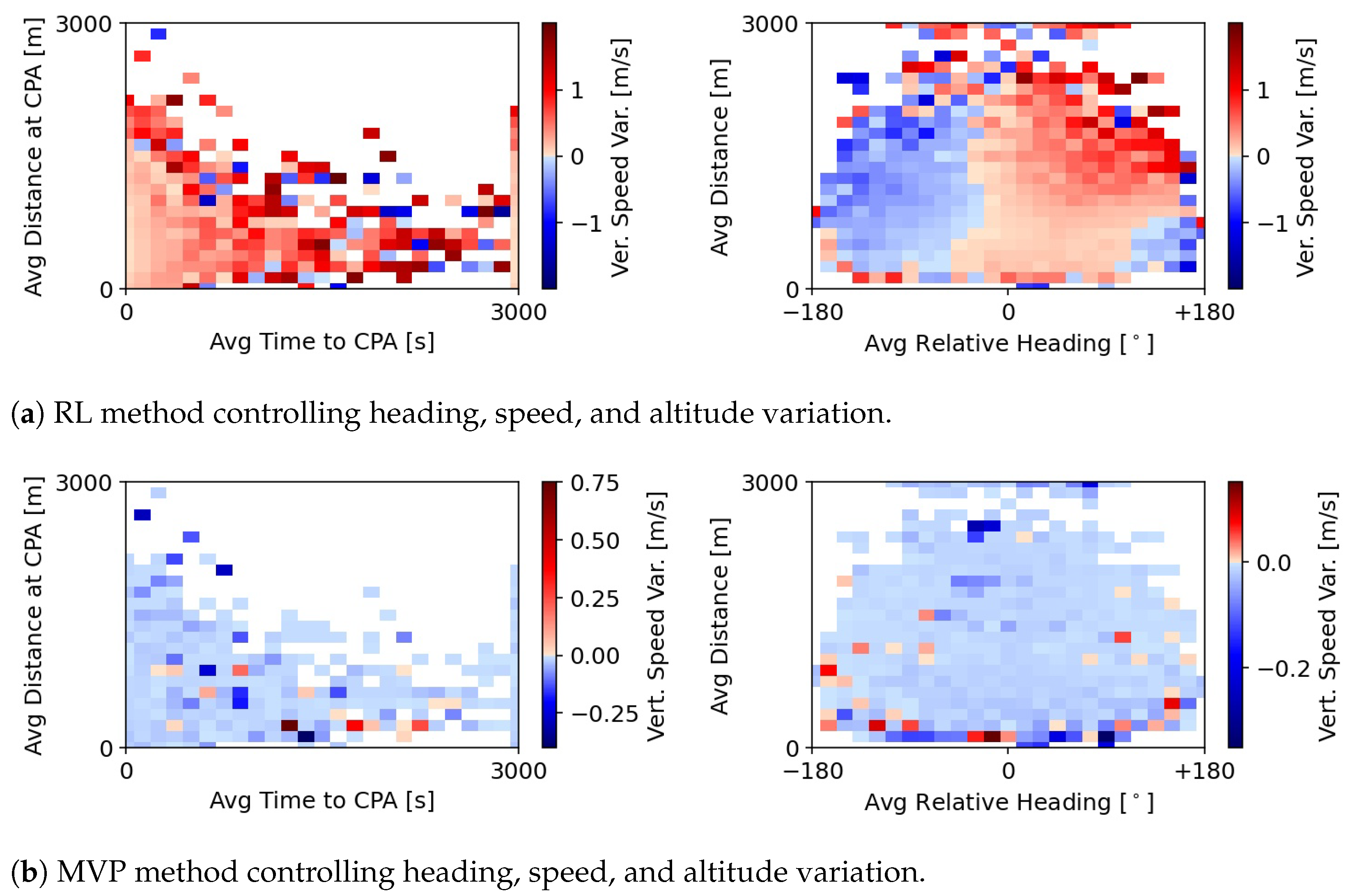
5.1.4. Vertical Speed Variation

Figure 9 displays the vertical speed variation performed by the RL and MVP methods when these control the heading, speed, and altitude variation. The RL method learnt to disperse aircraft quite efficiently, using climbing and descent actions almost equally. In practice, the RL method is creating three separated layers of traffic. MVP employs smaller vertical speed variations to resolve conflicts. Here, MVP is again more precise than the RL method, employing only the minimum altitude variation necessary to resolve conflicts. The RL method disperses aircraft more significantly through the airspace. This spread of traffic is likely to contribute to the reduction in conflicts and LoSs (see Figure 3a). However, it is likely to negatively affect flight path and time. This will be covered in more detail in the testing results in Section 5.2.3.

5.2. Testing of the RL Agent for Conflict Resolution

This section presents the testing phase of the RL method. The latter was tested with different traffic scenarios at a low, medium, and high traffic density. For each traffic density, three repetitions with three different route scenarios were run. The results of the RL method, related to safety, stability, and efficiency, are directly compared to those obtained when running the same traffic scenarios the MVP method.

5.2.1. Safety Analysis

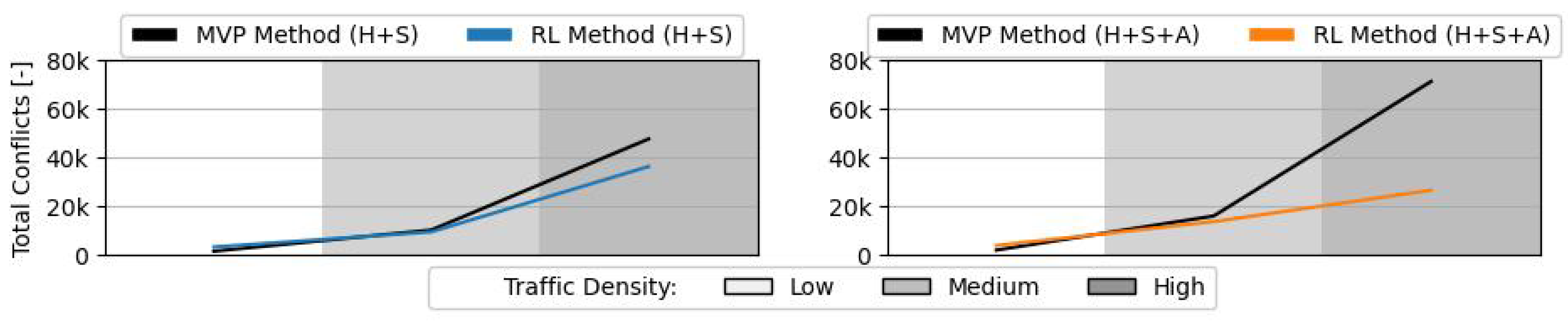
Figure 10 displays the average mean total number of pairwise conflicts. At low and medium traffic densities, the difference between the total number of conflicts with the RL and MVP methods is small, similar to the training results (see Figure 3b). With speed and heading deviation, there is a small difference at high traffic density, with the RL method achieving slightly fewer conflicts. Nevertheless, this is not a considerable difference. However, when altitude is also controlled, the RL method is capable of a great reduction in conflicts when compared to the MVP. This is probably a result of the larger altitude variations, as seen previously in Figure 9. These variations remove aircraft out of the main traffic layer both by climbing and descending, thus reducing the likelihood of secondary conflicts.

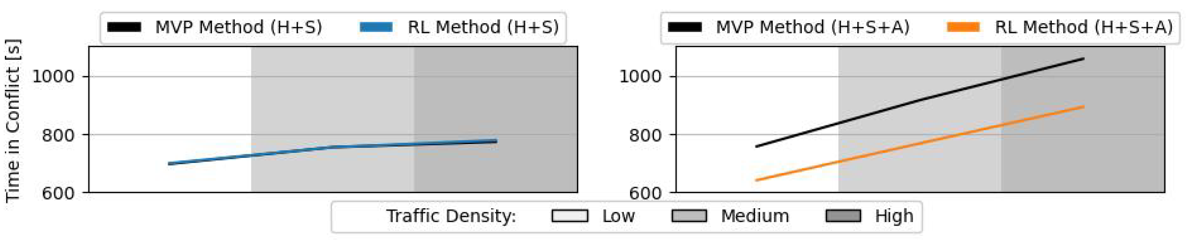
Figure 11 displays the average time in conflict per aircraft. An aircraft enters ‘conflict mode’ when it adopts a new state computed by the CR method. The aircraft will exit this mode once it is detected that it is past the previously calculated time to CPA (and no other conflict is expected between now and the look-ahead time). At this point, the aircraft will redirect its course to the next waypoint. The time to recovery is not included in the total time in conflict. Similar to the average total number of conflicts (see Figure 10), the total time in conflict is similar in both methods when these control heading and speed variation. In the H + S + A scenarios, with the RL method, aircraft spend less time in conflict at all traffic densities. Such is likely a result of the same choices in altitude variation that lead to a reduction in the total number of conflicts.

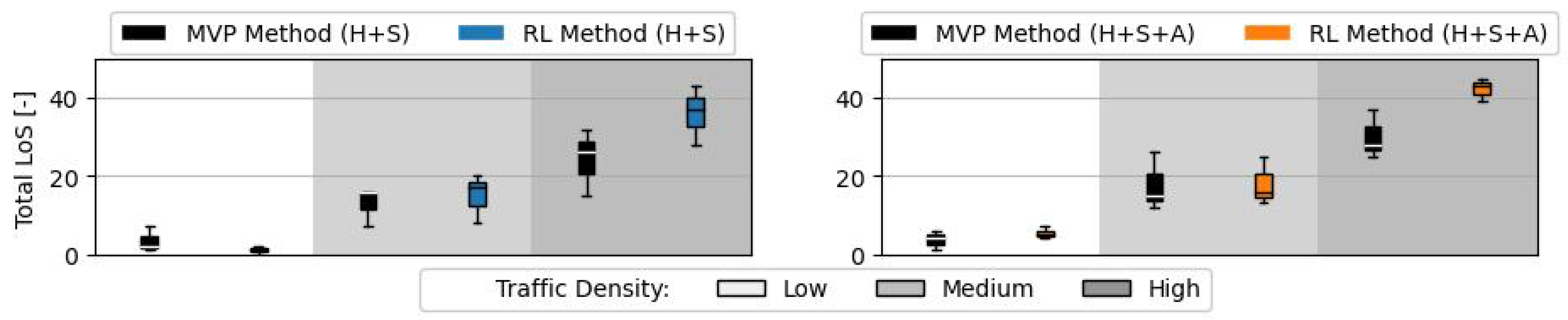
Figure 12 displays the total number of LoS. This is the paramount safety factor that the RL method aims to reduce. The RL method achieves a similar performance level at the medium traffic density independent of the action formulation, and an even stronger reduction in the number of LoSs at low traffic density when the methods control heading and speed variation. This is probably a result of the ‘defensive’ posture adopted by the RL method with far away intruders and close aircraft, as seen in Figure 5a. Head-on conflicts at relatively large distances, and nearby aircraft that can create imminent conflicts with only a small change in their velocity vector, can both be dangerous. However, this behaviour is not as efficient at higher traffic densities. Here, CR methods have to be more selective on the aircraft to defend against, as considering too many aircraft may result in a solution that does not fully resolve any conflict.

As hypothesised, the performance of the RL method deteriorated at a higher traffic density than that in which it was trained. Such can be a result of the small number of neighbouring aircraft considered in the state formulation. With a higher number of intruders per conflict geometry, the ownship will be ‘blind’ to part of the intruders. Limitation of the information in the state formulation limited the capability of the RL method to generalise the learnt behaviour to conflict geometries with more intruders. Additionally, it may be that different traffic densities require different resolution strategies: in this case, an RL method must be trained at least at the traffic density it will be used at.

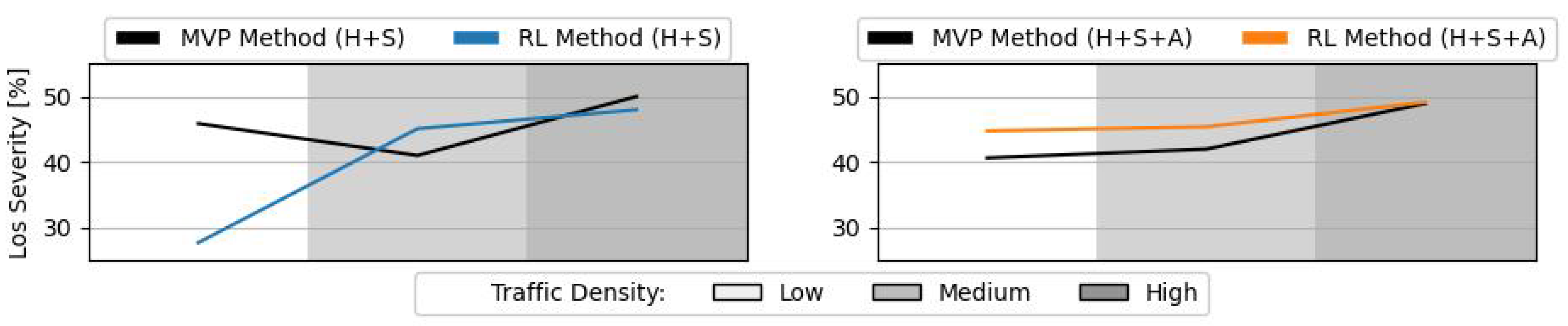
Figure 13 displays the average LoS severity. With heading and speed control, at low traffic densities, the RL method reduces the LoS severity on top of the total number of LoSs (see Figure 12). In all other situations, the average LoS severity is very similar. With all methods, there is a slight increase in the LoS severity as the traffic densities increases.

5.2.2. Stability Analysis

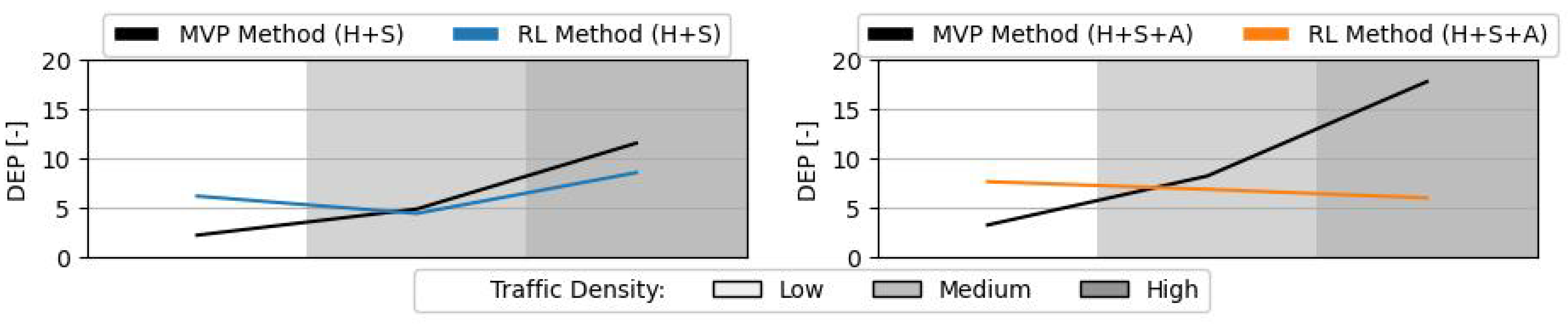
Figure 14 shows the average DEP value during the testing of the RL method. A high DEP symbolises a method that tends to create a larger number of secondary conflicts, resulting from large deviations with conflict resolution manoeuvres. With heading and speed control, the increase in the number of conflicts is negligible (as also seen in Figure 10). With additional altitude control, the RL method is better at preventing secondary conflicts than the MVP; which is also in line with the average total number of conflicts.

5.2.3. Efficiency Analysis

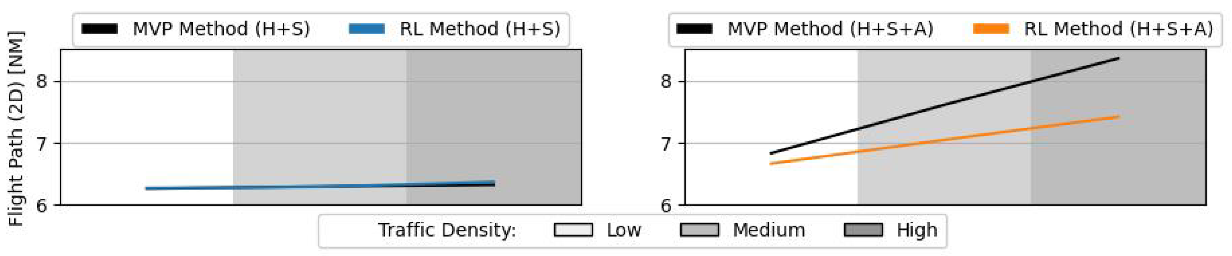
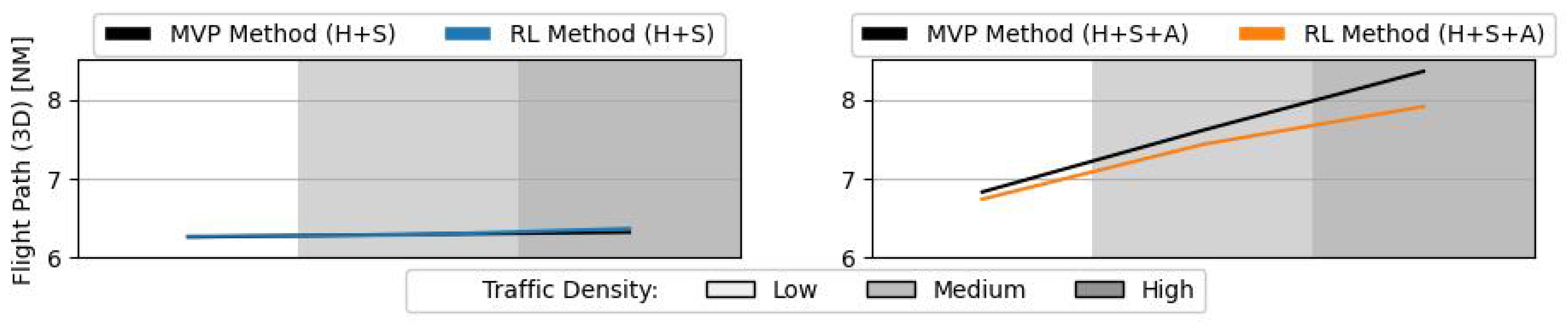
Figure 15 and Figure 16 show the average 2D and 3D flight path lengths per aircraft during testing of the RL method, respectively. There is only a noticeable difference between the RL and MVP methods, when altitude is also controlled. In this case, the RL method is able to reduce the increase in flight path resulting from tactical conflict manoeuvres, in comparison to the MVP method. Previously in Section 5.1.4, it was mentioned that the large vertical deviations performed by the RL method could have a negative effect on efficiency, by considerably increasing flight path length. However, it appears as though the decrease in total time in conflict (see Figure 11) may have counterbalanced these non-efficient vertical manoeuvres. As aircraft are able to spend more time travelling towards target and less time following a deconflicting state, the increase to the flight path is reduced.

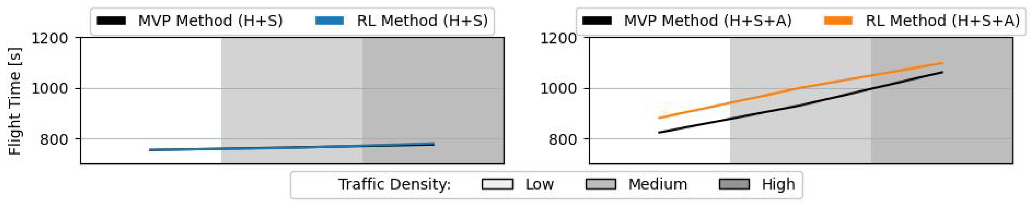
Figure 17 shows the average flight time per aircraft during testing of the RL method. The differences between the RL and MVP methods in efficiency with heading and speed control are again negligible. When the methods also performed altitude variation, there is a slight increase in the average flight time per aircraft. Since the method achieves a shorter flight path (see Figure 15 and Figure 16), the RL methods adopt on average lower horizontal speeds. This is in line with the speed variation decisions performed by the RL method during training (see Figure 7a), where, contrary to the MVP, it often opts for a decrease in horizontal speed.

6. Discussion

This work investigated whether RL methods can mitigate the undesirable global patterns emerging from successive conflict resolution manoeuvres in multi-actor conflicts, and improve safety compared to current geometric CR methods. The results obtained show that, at low traffic densities, RL methods can match, and sometimes even surpass, the performance of these geometric algorithms. The RL method learnt that the high number of conflicting aircraft force aircraft to frequently change their velocity vector. Defending in advance against nearby aircraft, even when not in conflict, has benefits given that a sudden change in the velocity vector can create imminent conflicts. Additionally, defending in advance against head-on conflicts, even when still at a large distance, may be crucial to prevent future LoSs.

However, performance deteriorates when these methods are exposed to traffic densities higher than those in which they were trained. The actions learnt from a set of conflict geometries, at smaller traffic densities, do not generalise well to conflict geometries with a higher number of intruders. This is a weakness of the approach. The benefit of RL is the potential to make generalisations about emerging patterns. If an RL method is only capable of creating a limited set of rules, its performance will be similar to that of geometric CR methods. Such may be a result of the limited information and variety of training scenarios provided to the RL method. Within the state representation, we considered a limit number of aircraft, which was found efficient within the specific training scenarios while still resulting in practicable convergence times. However, in conflict geometries with a higher number of intruders, the RL method may not have enough information to perform successful resolution manoeuvres. Thus, limiting state-action combinations may have a negative impact on the ability of RL methods to generalise solutions to different operational environments. Nevertheless, this limitation is often required to achieve convergence.

Naturally, it may also be that the RL method requires a longer training time, or even a more generalised training environment, than was provided in this work. Further testing is needed, with more information given to the method and more extensive training scenarios. However, it should also be taken into account that doing so heavily increases the necessary training time of the method. Notwithstanding, the actions performed by the RL method in this study can provide guidelines on how to improve the performance of current geometric CR methods. This topic, as well as further analysis of the actions performed by the RL method, is addressed in the following sections.

6.1. Actions Performed by the Reinforcement Learning Method

This work proved that an RL method can successfully resolve conflicts and prevent losses in minimum separation. Furthermore, having a global reward improved action coordination between aircraft. The actions of the RL method are the result of the combination of multiple factors. However, results show that the current distance to aircraft and relative heading have a bigger impact on the method’s decisions than, for example, the distance at the closest point of approach. This is possibly because the method was able to establish that small distances between aircraft result in negative rewards. Additionally, the method learnt that head-on conflicts are especially hard to resolve in the short-term. Finally, by observing all actions performed during training, it is clear that the RL method has a preference for always turning one direction when resolving conflicts. Although this is a very simple coordination rule, it is efficient in pairwise conflicts. However, it is likely that a better coordination rule is necessary when more aircraft are involved in a conflict situation. Such might explain why the performance of the RL method deteriorated at higher traffic densities.

Moreover, with three degrees of freedom (i.e., heading, speed, and altitude), the RL method achieved fewer conflicts and LoSs than with 2 degrees of freedom (i.e., heading, and speed). This is unexpected, since larger actions formulations are often negative for RL methods, as it increases the possible combinations of state-action that the method must learn and adapt to. However, the improvement in resolution manoeuvres is intrinsically related to best practices for conflict resolution. With more degrees of freedom, the method learnt to perform smaller deviations on each. This reduces the amount of airspace that the ownship occupies during a deconflicting manoeuvre, thus also reducing the likelihood of colliding with other aircraft. Additionally, given the characteristics of the operational environment in this work, where all aircraft travel in one layer, fast singular vertical manoeuvres can be very efficient in resolving conflicts. The RL method took advantage of this fact. It is likely that the RL method would find different optimal options in an environment with different characteristics, e.g., a layered airspace.

6.2. Rules for Conflict Resolution

Reinforcement learning applications are often a ‘black-box’; the reasons for their choices are often not clear or predictable. However, if these are to be certified as safety critical systems, we must find ways to make their behaviour interpretable and traceable. Many researchers also defend that we should look at RL methods as a source of best practices. These practices can then be implemented in human-built CR methods, whose actions are pre-defined and can be trusted upon. With this implementation in mind, and considering the behaviour of the RL method in this work, the following rules for improving geometric CR methods can be derived:

• The RL method often prioritised the current distance to aircraft over the distance at CPA. Nearby aircraft can potentially change their course and immediately turn into an (almost) impossible to resolve conflict. Geometric CR methods often simply look at the distance at CPA, and the time to CPA. Nearby aircraft, even if not in conflict, should be defended against.
• The RL method defends against head-on conflicts in advance. Based on the results, the RL method also performs strong state variations when intruders are far away, but (near-)head-on. Short-term head-on conflicts can only be resolved with coordinated sharp heading turns. When the intruder is farther away, smaller heading deviations are needed to resolve the conflict. Geometric CR methods initiate deconflicting actions for all conflict situations in the same manner, i.e, when these are within a pre-defined look-ahead time. However, the decision of when a resolution manoeuvre is initiated, should be made in regard to the relative geometry between the ownship and the intruder. In practice, different rules for look-ahead times could be implemented per relative heading.

In summary, the RL method adopts a more preventive/cautious position towards nearby aircraft, even when not in conflict, and defends in advance against severe conflict geometries. However, given the results obtained, it may be that the previous rules are more efficient at low traffic densities where there is enough space. The previous measures resulted in the method defending against more aircraft, per deconflicting action, than a typical geometric CR method would have. At higher traffic densities, it may be that such behaviour results in too high a number of conflicts that saturate the solution space.

6.3. Future Work

The present work should be extended to different operational environments. Comparison of the optimal manoeuvres performed by RL methods trained in different environments provides valuable information. First, it aids in the identification of potential risks in each type of operation. Second, it helps identify a global optimal usage of reinforcement learning towards improving safety in aviation. In particular, the following is suggested for future work:

• It may be that different traffic densities require different resolution strategies, as was also hypothesised in the Metropolis project [16]. In this case, the RL method must learn different responses per complexity of emergent behaviour resulting from increasing traffic densities. RL methods should be tested at different traffic densities, and their actions compared, before they can be implemented in a real-world scenario.
• With heading and speed control only, the RL method employed large heading deviation which led to a high number of secondary conflicts. This may be because all losses of minimum separation are valued the same. The method may benefit from having additional distance between aircraft to prevent negative rewards. As a possible solution, less weight could be given to minor, less severe LoSs. Such could potentially lead the method to adopt smaller state changes, running the risk of scraping the protected zone of intruders over large deconflicting manoeuvres that would place the ownship in the direct path of other aircraft.

7. Conclusions

Reinforcement learning (RL) bears the potential to adapt to the detrimental emergent behaviour from multi-actor conflicts, and knock-on effects from successive conflict resolution manoeuvres, that occur as traffic densities increase. An RL method can potentially develop a large set of rules, adapted to different conflict geometries, from knowledge of the environment captured during training. Adding to the success of RL approaches in other scientific areas, this paper has shown that RL methods can be used to guarantee minimum separation between all operating aircraft in an unmanned aviation environment.

The RL method herein developed successfully resolved conflicts and reduced the number of losses in minimum separation (LoSs). Moreover, it matched, and at lower traffic densities even surpassed, the performance of a state-of-the-art geometric conflict resolution (CR) algorithm. The advantage of an RL method is the ability to learn safe procedures, beyond the limitations of a fixed set of rules, as implemented with geometric CR methods. However, there are still some weaknesses to this approach. The performance of the RL method deteriorated when exposed to traffic densities higher than those in which it was trained. The RL method receives limited information from the environment, in order to limit the number of possible state-action combinations. It is likely that this also limited its ability to generalise its solutions to different operational environments.

Additionally, RL methods can inspire the creation of additional rules/guidelines to improve the performance of geometric CR algorithms. How RL methods resolve conflicts in different environments can help identify the risks in every type of operation, as well as possible solutions. In this specific work, the RL method showed that: (1) adopting a more ‘preventive’ position towards nearby aircraft, even when not in conflict, and (2) defending in advance against difficult conflict geometries, help prevent LoSs at low traffic densities.

Next steps will focus on further exploring state and action formulations in order to increase the efficacy of the RL method at higher traffic densities than the one it is trained in. Furthermore, related studies should extend the training and testing of conflict resolution RL methods to different operational environments. Different methods, with different amounts of information and control, should be applied and compared. Such will make it possible to evaluate the influence of these parameters in the method’s capability to generalise and identify conflict geometry-specific solutions. Nevertheless, these decisions must be evaluated together with the consequent necessary training time, and resources, for the method to converge towards optimal actions.