Filtering and Estimation of State and Wind Disturbances Aiming Airship Control and Guidance

Abstract

Good state and wind estimation is a requirement for the development of guidance and control techniques for airships. However, usually this information is not directly available from the airship sensors. The typical solution applies filtering, estimation and sensor fusion methods. This paper presents a comparative study, evaluating three solutions for the state estimation of NOAMAY airship. We also present alternative versions for the crucial estimation of the wind velocity, combining Kalman filters with a data-driven Neural Network. Finally, we present special solutions to usual problems encountered in filtering implementation as the mitigation of delays caused by second-order filters. The sensors set considered is composed of a global positioning system, an inertial measurement unit and a one-dimensional Pitot probe. Comparative simulation results are presented with the use of a realistic nonlinear model of the airship.

1. Introduction

Airships with autonomous operation capability are in the focus of worldwide investigation. Airships are particularly suited to scenarios that demand long endurance, high payload and low operational risk, such as surveillance and environmental monitoring [1].

Airship control is a big challenge for the control systems designers as they are underactuated vehicles with strong nonlinear undamped dynamics [2]. Further, many nonlinear control approaches like sliding mode, backstepping and incremental dynamic inversion require the knowledge of vehicle velocities and accelerations, that may not be available from sensors [3]. Thus, an accurate estimation of the state and its derivatives is fundamental to the design of efficient control and guidance techniques.

Another crucial point is the wind estimation, which is particularly important for lighter-than-air vehicles [4,5]. The work of [6] showed that a good wind knowledge can result in more accurate geolocation of a ground target. Additionally, the crab-angle between ground track and heading, obtained from estimating the wind conditions, can improve the control performance of an airship in trajectory following. Finally, when the objective is ground-hover at constant altitude, the blimp must align itself against the wind and use its forward propulsion to balance the aerodynamic drag [7]. Therefore, by knowing the wind speed and direction control performance can be improved.

For both state and wind estimation, the solution relies on filtering, estimation and fusion of the sensory data. Common approaches are the Extended Kalman Filter (EKF) and the Unscented Kalman Filter (UKF). As an example, in [8], it is proposed an approach for estimating the angle of attack and sideslip angle by the kinematic equations of motion of an aerobatic UAV. Meanwhile, with the same kinematic equations, in [6] an extended Kalman flter (EKF) is proposed for estimating the wind heading and velocity using an aircraft with a single GPS and Pitot tube. In [9], a wind velocity observer also based on the kinematics is proposed for small UAVs with experimental results. Similarly, in [10] is also proposed an EKF for wind velocity estimation, however applied to a stationary stratospheric airship in simulation environment. Then in [11] are presented four model-based solutions considering an aircraft with four diferent possible configurations of sensors, as is shown in Figure 1.

This work is placed in the context of project InSAC https://www2.eesc.usp.br/insac accessed on 25 May 2022. The project aims to develop an autonomous airship for performing environmental monitoring tasks in remote Amazon rain forest areas. Such tasks include aerodynamic flights and ground-hover (i.e., keep a stationary position with respect to a ground target).

Firstly, the paper presents a comparative study evaluating different different solutions for the state/derivatives estimation of NOAMAY airship, which is instrumented with a pitot tube and an Inertial Measurement Unit (IMU) including: accelerometer, gyroscopes, GPS, barometer and thermometer.

In a second moment, for the wind estimation, this work presents an alternative version of a model based on wind velocity estimator using the EKF combined with a data-driven approach of estimation using a Neural Network (NN). The main tool to validate the proposed estimation approaches is a dynamical realistic nonlinear model of an airship in Simulink/MATLAB. This tool is a result of the research group efforts since the seminal project AURORA, which was improved during the projects DIVA and DRONI [12].

Finally, we present possible solutions to mitigate common problems arriving in filtering implementation like the control input redundancy and the delays caused by second-order filters [3]. For the input redundancy, related to an overactuated control system, we propose filtering the less important commanded input, an approach that is known as Washout Filter (WOF) [13]. Another critical point is the drawback that appears in the second-order filters used to estimate state derivatives. The natural dynamics delay produced by these filters may harm the control system feedback. One possible solution to mitigate this delay is the so called Input Scaling Gain (ISG), that was first proposed by our research group in 2015 as a scalar factor gain [14]. In this paper, we generalize the input scale gain to the MIMO case. To illustrate these two design solutions we present briefly the concept of incremental controllers, that are used to show the benefits of these filtering techiques, although not limited to these kind of controllers.

2. Airship Model

The main tool to validate the proposed control approach is a dynamical realistic nonlinear model of a robotic airship, which can be expressed in a state-space form as following:

$$\dot{\xi }=g(\xi ,\mathbf{x},\mathbf{d}),$$

(1a)

$$\dot{\mathbf{x}}=f(\xi ,\mathbf{x},\mathbf{d},\mathbf{u}),$$

(1b)

where:

• the kinematic states $\xi ={\left[{\mathbf{P}}^{\mathbf{T}}{\mathbf{\Phi }}^{\mathbf{T}}\right]}^{\mathbf{T}}$ include the cartesian position $\mathbf{P}={\left[P_N{P}_E{P}_D\right]}^T$ and angular position $\mathbf{\Phi }={\left[\varphi \theta \psi \right]}^T$ in the North-East-Down (NED) frame (SI units);
• the dynamic states $\mathbf{x}={\left[{\mathit{V}}^{\mathbf{T}}{\mathbf{\Omega }}^{\mathbf{T}}\right]}^{\mathbf{T}}$ include the linear speed $\mathit{V}={\left[uvw\right]}^T$ and angular speed $\mathbf{\Omega }={\left[pqr\right]}^T$ in the body frame (SI units);
• the input vector $\mathit{u}={\left[{\delta }_e{\delta }_a{\delta }_r{\delta }_0{\delta }_q{\mu }_0\right]}^T$ includes: ${\delta }_e,{\delta }_a$ and ${\delta }_r$ which are elevator, aileron and rudder deflections; ${\delta }_0$ as the normalized thrusters voltage; ${\delta }_q$ as the differential voltage between the front-back thrusters; ${\mu }_0$ as the common vectoring angle of the thrusters;
• and, finally, the disturbance vector $\mathbf{d}$ that includes wind velocities and gust variables (SI units), as is shown in Figure 2.

The dynamics are based on Newton-Euler equations considering the body frame centered in the Center of Buoyancy (CB), which is approximately equivalent to the Center of Volume (CV) [12]. Further, some nonlinear effects are included in the simulation, such as: atmospheric pressure variation, temperature variation, lifting gas pressure variation, Coriolis effect and actuator nonlinearities [7].

Finally, the linear and angular positions are updated through kinematic equations as follows:

$$g(\xi ,\mathbf{x})=\left[\begin{array}{cc}{\mathbf{S}}_{\mathbf{\Phi }}^{\mathbf{T}}& 0_{3\times 3}\\ 0_{3\times 3}& {\mathbf{R}}_{\mathbf{\Phi }}^{\mathbf{T}}\end{array}\right]\left[\begin{array}{c}{\mathbf{V}}_{\mathbf{g}}\\ \mathbf{\Omega }\end{array}\right],$$

(2)

where $0_{3\times 3}$ is a null matrix of 3th order, ${\mathbf{S}}_{\mathbf{\Phi }}\in {\mathbf{R}}^{\mathbf{3}\times \mathbf{3}}$ is the rotational matrix from airship body to NED frame, and ${\mathbf{R}}_{\mathbf{\Phi }}\in {\mathbf{R}}^{\mathbf{3}\times \mathbf{3}}$ is the angular transformation matrix, both given by [7]:

$${\mathbf{S}}_{\mathbf{\Phi }}=\left[\begin{array}{ccc}{\mathrm{c}}_{\psi }{\mathrm{c}}_{\theta }& {\mathrm{s}}_{\psi }{\mathrm{c}}_{\theta }& -{\mathbf{s}}_{\theta }\\ {\mathrm{c}}_{\psi }{\mathrm{s}}_{\theta }{\mathrm{s}}_{\varphi }-{\mathrm{s}}_{\psi }{\mathrm{c}}_{\varphi }& {\mathrm{s}}_{\psi }{\mathrm{s}}_{\theta }{\mathrm{s}}_{\varphi }+{\mathrm{c}}_{\psi }{\mathrm{c}}_{\varphi }& {\mathrm{c}}_{\theta }{\mathrm{s}}_{\varphi }\\ {\mathrm{c}}_{\psi }{\mathrm{s}}_{\theta }{\mathrm{c}}_{\varphi }+{\mathrm{s}}_{\psi }{\mathrm{s}}_{\varphi }& {\mathrm{s}}_{\psi }{\mathrm{s}}_{\theta }{\mathrm{c}}_{\varphi }-{\mathrm{c}}_{\psi }{\mathrm{s}}_{\varphi }& {\mathrm{c}}_{\theta }{\mathrm{c}}_{\varphi }\end{array}\right],$$

$${\mathbf{R}}_{\mathbf{\Phi }}=\left[\begin{array}{ccc}1& {\mathrm{s}}_{\varphi }{\mathrm{t}}_{\theta }& {\mathrm{c}}_{\varphi }{\mathrm{t}}_{\theta }\\ 0& {\mathrm{c}}_{\varphi }& -{\mathrm{s}}_{\varphi }\\ 0& {\mathrm{s}}_{\varphi }/{\mathrm{c}}_{\theta }& {\mathrm{c}}_{\varphi }/{\mathrm{c}}_{\theta }\end{array}\right],$$

where ${\mathrm{c}}_x=cos\left(x\right)$, ${\mathrm{s}}_x=sin\left(x\right)$ and ${\mathrm{t}}_x=tan\left(x\right)$.

3. Sensors Modeling

In this section, a summary of the sensors modeling is presented, including manufacturer specifications, such as bias and sample frequency. The NOAMAY robotic airship is instrumented with a set of sensors including a Pitot Tube, responsible for measuring the airspeed ($V_{pitot}$) and a multi-sensor Xsens Mti-G 700 which provides the following information [15]:

• absolute position ${\mathbf{P}}_{\mathbf{NED}}$ [m] measured by GPS;
• absolute orientation in the world $\mathbf{\Phi }$ [rad], as result of a sensor fusion between Gyroscope and Magnetometer;
• inertial linear velocity (${\mathbf{V}}_{\mathbf{g}}$) in three-axis [m/s], estimated by the GPS;
• inertial angular velocity ($\mathbf{\Omega }$) in three-axis [rad/s], estimated by the IMU;
• inertial acceleration in three-axis ($\mathit{a}={\left[a_x{a}_y{a}_z\right]}^T$) [m/s${}^2$], measured by the Accelerometer;
• atmospheric pressure $P_h$ [hPa], by the barometer;
• and temperature $T_h$ [K], measured by the thermometer.

The sample frequency of the sensors are shown in the

Table 1. Sample frequency specification.

Sensor	Frequency [Hz]	Sampled Data
IMU	100	$\mathbf{\Phi }$, $\mathbf{\Omega }$, $\mathit{a}$
GPS	4.00	${\mathbf{V}}_{\mathbf{g}}$, ${\mathbf{P}}_{\mathbf{NED}}$
Barometer	50.0	$P_h$
Thermometer	1.00	$T_h$

. Further, a first order model for the Gauss Markov error of each sensor is given as [16]:

$$y=\widehat{y}+b+w_y$$

(3a)

$$\dot{b}=-\frac{1}{\tau }b+w_b$$

(3b)

where b is the sensor bias with Gaussian noise $w_b$, $w_y$ is a Gaussian noise for the measure as shown in

Table 2. Sensor noise specification ($w_y$).

Data	${\mathit{\sigma }}_{\mathit{RMS}}$	Data	${\mathit{\sigma }}_{\mathit{RMS}}$
$\varphi ,\theta$ [rad]	0.00520	$\mathit{a}$ [m/s${}^2$]	0.0040
$\psi$ [rad]	0.10000	$P_N,P_E$ [m]	2.5000
$P_D$ [m]	5.00000	$V_{pitot}$ [m/s]	0.0020
$\mathbf{\Omega }$ [rad/s]	0.00035	${\mathbf{V}}_{\mathbf{g}}$ [m/s]	0.4000
$P_h$ [hPa]	0.01000	$T_h$ [K]	1.0000

, $\widehat{y}$ is the true simulated value and y is the corresponding sensor output. For the sensors presenting bias, the parameter ${\sigma }_{RMS}$ (The noise power is given by ${\left({\sigma }_{RMS}\right)}^2/$(sample frequency)) is specified in

Table 3. Sensor bias specification ($w_b$).

Sensor	${\mathit{\sigma }}_{\mathbf{RMS}}$
Gyroscope [${}^{\circ }/s$]	1.3$·{10}^{-4}$
Accelerometer [m/s${}^2$]	2.3$·{10}^{-5}$
Barometer [hPa]	1.4$·{10}^{-5}$

. In the case of Accelerometer, Barometer and Thermometer there are some special parameters shown below.

For the case of pose measurement a coordinate transformation is applied to the data (with translational and rotational components). The GPS output is modeled as following:

$${\mathbf{P}}_{{\mathbf{gps}}_{\mathbf{k}}}={\mathbf{S}}_{\mathbf{xsens}}({\mathbf{P}}_{{\mathbf{NED}}_{\mathbf{k}}}+{\mathbf{P}}_{\mathbf{xsens}})+{\mathbf{\phi }}_{{\mathbf{pos}}_{\mathbf{k}}},$$

(4)

where: ${\mathbf{S}}_{\mathbf{xsens}}$ is the rotational matrix from the CB angular pose to the Xsens angular pose; and ${\mathbf{P}}_{\mathbf{xsens}}$ is the Xsens position in the body frame; ${\phi }_{{pos}_k}$ is a position Gaussian noise vector at instant k; and ${\mathbf{P}}_{{\mathbf{gps}}_{\mathbf{k}}}$ is the sampled position given by the GPS at instant k.

The orientation output is modeled as following:

$${\mathbf{\Phi }}_{{imu}_k}={\mathbf{\Phi }}_{xsens}+{\mathbf{\Phi }}_k+{\mathbf{\phi }}_{{ori}_k},$$

(5)

where: ${\mathbf{\Phi }}_k$ is the orientation given in simulation at instant k; ${\mathbf{\Phi }}_{xsens}$ is the Xsens angular pose in the body frame; ${\mathbf{\phi }}_{{ori}_k}$ is an orientation Gaussian noise vector at instant k; and ${\mathbf{\Phi }}_{{imu}_k}$ is the sampled angular position given by IMU at instant k.

For the velocity measurement, we apply the coordinate transformation to the data (with rotational components).

The resulting linear velocity output is as follows:

$${\mathbf{V}}_{{\mathbf{gps}}_{\mathbf{k}}}={\mathbf{S}}_{\mathbf{xsens}}({\mathbf{V}}_{{\mathbf{g}}_{\mathbf{k}}}+{\mathbf{\Omega }}_{\mathbf{k}}\times {\tilde{\mathbf{O}}}_{\mathbf{xsens}})+{\mathbf{\phi }}_{{\mathbf{vel}}_{\mathbf{k}}},$$

(6)

where: ${\mathbf{\Omega }}_k$ is the angular velocity given in simulation at instant k; ${\tilde{\mathbf{O}}}_{\mathbf{xsens}}$ is the position vector from the CB to the Xsens position; ${\mathbf{S}}_{\mathbf{xsens}}$ is the rotational matrix from the CB angular pose to the Xsens angular pose; and ${\mathbf{P}}_{\mathbf{xsens}}$ is the Xsens position in the body frame; ${\mathbf{\phi }}_{{vel}_k}$ is a position Gaussian noise vector at instant k; and ${\mathbf{P}}_{{\mathbf{gps}}_{\mathbf{k}}}$ is the sampled position given by the GPS at instant k.

The angular velocity output is modeled as following:

$${\mathbf{\Omega }}_{{imu}_k}={\mathbf{S}}_{\mathbf{xsens}}{\mathbf{\Omega }}_{\mathbf{k}}+{\mathbf{\phi }}_{{\mathbf{rate}}_{\mathbf{k}}},$$

(7)

where: ${\mathbf{\phi }}_{{rate}_k}$ is an angular velocity Gaussian noise vector at instant k; and ${\mathbf{\Omega }}_{{imu}_k}$ is the sampled angular velocity given by the IMU at instant k.

The accelerometer signal includes the additional components of centripetal acceleration ($a_c$) and gravitational acceleration ($a_g$), as:

$$\mathit{a}={\dot{\mathbf{V}}}_g+\dot{\mathbf{\Omega }}\times {\tilde{\mathbf{O}}}_{\mathbf{xsens}}-{\mathbf{S}}_{\mathbf{\Phi }}{\mathbf{a}}_{\mathbf{g}}+{\mathit{a}}_{\mathbf{c}},$$

(8)

where ${\tilde{\mathbf{O}}}_{\mathbf{xsens}}$ is the vector from the CB to the sensor location, ${\mathrm{S}}_{\mathsf{\Phi }}$ is the rotation matrix from the body frame to the North-East-Down frame and ${\mathit{a}}_c=\mathbf{\Omega }\times (\mathbf{\Omega }\times {\tilde{\mathbf{O}}}_{\mathbf{xsens}})$.

In the case of the static pressure at a given altitude, we use the International Standard Atmosphere (ISA):

$$P_h=P_0{\left(\frac{T_h}{T_h-0.0065P_D}\right)}^{5.257},$$

(9)

where $P_h$ is the static pressure, $T_h$ is temperature in Kelvin, $P_D$ is the negative of the altitude (in meters) in the inertial frame and $P_0$ is the pressure at zero altitude (at the sea level $P_0=101.325$ hPa).

The temperature is given by the classical model, as linearly varying with the altitude:

$$T_h=T_0+0.0065P_D,$$

(10)

where $T_0$ is the temperature at zero altitude, recalling that $P_D$ is negative in our model.

4. Filtering and Estimation

We present here three possible solutions for the estimation of the state variables of an airship, with particular analysis for the NOAMAY airship. The first one is the classical second-order filter, and the other two are Kalman Filters (EKF and UKF). The performances of the three approaches are then analyzed and compared. The algorithms developed in C/C++ using the Robotic Operating System (ROS) [17], are available for consulting.

4.1. Low-Pass Filter

The first estimator is the classical second-order Low-pass filter (LPF), defined as:

$$\frac{\chi \left(s\right)}{Y\left(s\right)}=\frac{{\omega }_f^2}{s^2+2{\omega }_f\zeta s+{\omega }_f^2},$$

(11)

where $\chi \left(s\right)$ is the estimated state, $Y\left(s\right)$ is the sensor measure, ${\omega }_f$ is the cut-off frequency and $\zeta$ is the damping coefficient. For each estimated state and corresponding sensor, the filter parameters used here are given in the

Table 4. Configuration for Low-pass filter.

State	Sensor	${\mathit{\omega }}_{\mathit{f}}$ [rad/s]	$\mathit{\zeta }$
${\mathbf{P}}_{\mathbf{NED}}$, ${\mathbf{V}}_{\mathbf{g}}$	GPS	3.33	0.96
$\mathbf{\Phi }$, $\mathbf{\Omega }$	IMU	10	0.96

. These values were chosen during simulation by manual tuning.

4.2. Extended Kalman Filter

The EKF algorithm is probably the most popular estimator used in the literature. In this work we use the EKF ROS package (Available https://wiki.ros.org/robot_localization accessed on 25 May 2022) known as robot_localization) [18]. This package is related to the configuration of a generic 6DOF mobile robot with 6-DOF, yielding the filtered estimation of positions, velocities and accelerations, both linear and angular.

We want to estimate here the complete airship state vector (${\mathbf{P}}_{\mathbf{NED}},\mathbf{\Phi },{\mathbf{V}}_{\mathbf{g}},\mathbf{\Omega },\mathit{a}$). Thus, the measurement update stage uses the sensors output, as described in

Table 5. Configuration for measurement update stage.

Data∖Sensor	GPS	IMU	Barometer
$P_{NED}$	1	0	0
$\mathsf{\Phi }$	0	1	0
u, v	1	0	0
w	1	0	1
$\mathsf{\Omega }$	0	1	0
$\mathit{a}$	0	1	0

, where 1 indicates the presence of the sensor in the corresponding measured variable while 0 is the opposite.

One important feature of robot_localization package is the sensor-based frame reference in the East-North-Upper (ENU) frame, while we use the Norht-East-Down (NED) frame, requiring a conversion. Further, regarding the acceleration signal, we implement a cascaded approach in order to remove the centripetal acceleration component, as:

$${\widehat{\dot{\mathbf{V}}}}_g=\mathit{a}-{\widehat{\mathbf{\Omega }}}_0\times ({\widehat{\mathbf{\Omega }}}_0\times {\tilde{O}}_{xsens}),$$

(12)

The weights of the diagonal covariance matrix ($15\times 15$) of the process are shown in

Table 6. Process covariance matrix.

State	Weight	State	Weight
$\mathsf{\Phi }$ [rad]	0.010	$\mathit{a}$ [m/s${}^2$]	0.100
$\mathsf{\Omega }$ [rad/s]	0.100	$u,v$ [m/s]	0.050
$P_N$ [m]	0.001	$P_E$ [m]	0.001
$P_D$ [m]	0.010	w [m/s]	0.001

. The gains were chosen empirically, considering that the vehicle has slow dynamics and that the airship can be assumed to be a rigid body. The hypothesis of enough stiffness of the hull is true if we consider that the envelope is under full operational volume and pressure [19,20,21]. The rigidity assumption of a conventional airship is broken for extremely high speeds or if the envelope is made of thin films to reduce the weight [22,23], which is not the case of the NOAMAY airship.

4.3. State Estimation Results

We show here the simulation results comparing the three approaches, for the state estimation in a trajectory tracking control case, as developed in [3]. The sampling rate of the estimators is 32 Hz and the wind is blowing from the North. A visualization of the estimation results, made in Simulink/Matlab, are available in youtu.be/VL5dvCyOZwY (EKF) and youtu.be/B26xaKtAyWo (UKF) accessed on 25 May 2022.

Figure 3(above) shows the estimated trajectories for the different estimators, from which we can see that EKF appears to be smoother and with less errors. The signals of the longitudinal (u), vertical (w) and angular velocity in z-axis (r) appear in Figure 3(down). We can see that the classical LPF provides good filtering, but with a significant delay, while UKF is faster though with a bigger error. The EKF filter has a time response similar to the UKF case, while displaying lower errors.

Thus, for the airship model considered here, the EKF showed a better performance in comparison to UKF and LPF. For further details, including the RMS values of the position errors, please refer to [3]. These results show the natural compromise between noise attenuation versus estimation delay, found in an estimator design.

5. Wind Velocity Estimators

This section addresses the problem of wind velocity estimation. Firstly, we detail the equations related to the wind (${\mathbf{V}}_{\mathbf{w}}$) and inertial airship velocities (${\mathbf{V}}_{\mathbf{g}}$), as well as the airship orientation ($\mathbf{\Phi }$), which are related to the Pitot probe sensor.

Let us define the airship’s relative velocity (${\mathbf{V}}_{\mathbf{a}}$), or airspeed, as:

$${\mathbf{V}}_{\mathbf{a}}={\mathbf{V}}_{\mathbf{g}}-{\mathbf{V}}_{\mathbf{w}},$$

(13)

Whose modulus is called true airspeed ($V_t$) and is given by:

$$V_t=\left|\right|{\mathbf{V}}_a{\left|\right|}_2=\sqrt{u_a^2+v_a^2+w_a^2}.$$

(14)

Let us recall also the aerodynamic angles, the sideslip $\beta$ and the angle of attack $\alpha$, as shown in Figure 4, defined by:

$$\beta ={sin}^{-1}\frac{v_a}{V_t},$$

(15)

$$\alpha ={tan}^{-1}\frac{w_a}{u_a}.$$

(16)

Or, equivalently:

$$w_a=u_a\frac{sin\alpha }{cos\alpha }\mathrm{and}{v}_a=V_{t}sin\beta .$$

(17)

Finally, we obtain:

$$V_t=\frac{u_a}{cos\alpha cos\beta }.$$

(18)

The Pitot tube is located at the airship nose (see Figure 2). Also, the airship has a pressure sensor connected to the Pitot Tube. Thus, as the airship moves forward, the longitudinal dynamic pressure $\Delta P$ will be measured by the pressure sensor. The relation between the measured pressure and the airship longitudinal airspeed can be derived from Bernoulli’s equation as shown by [6], which can be rewritten as below:

$$\Delta P=\eta {\left(u_a\right)}^2,$$

(19)

where $\eta$ is the calibrating factor related to the air density and pitot efficiency. Now, if we use the variable transformation below:

$$V_{pitot}=\sqrt{\Delta P},$$

(20)

And using the statements (18) and (20), we can rewrite (19) as below:

$$V_t=\frac{V_{pitot}}{\sqrt{\eta }cos\alpha cos\beta }.$$

(21)

The unknown parameters in $\eta$ together with the inaccurate angle values $\alpha$ and $\beta$ are then estimated together in a single variable, or scale factor $c_f$, given by:

$$c_f=\sqrt{\eta }cos\alpha cos\beta ,$$

(22)

And thus (21) is now given by:

$$V_t=\frac{1}{c_f}{V}_{pitot}.$$

(23)

Now, recalling that ${\mathbf{V}}_{\mathbf{g}}$ is written in the body, as well as ${\mathbf{V}}_{\mathbf{a}}$, if we take these vectors written in the inertial frame (NED), we can write the relative velocity equation (13) using the rotational matrix ${\mathbf{S}}_{\mathbf{\Phi }}$ from airship body to NED frame, we have:

$${\mathbf{V}}_{\mathbf{NEDa}}={\mathbf{V}}_{\mathbf{NED}}-{\mathbf{V}}_{\mathbf{NEDw}}={\mathbf{S}}_{\mathbf{\Phi }}^{\mathbf{T}}{\mathbf{V}}_{\mathbf{a}}.$$

(24)

As the rotational operation does not change the vector modulus, and assuming a wind speed in the North-East plane, we have:

$$V_{pitot}^2=c_f^2({(V_N-V_{N_w})}^2+{(V_E-V_{E_w})}^2+{(V_D)}^{)}).$$

(25)

Assuming initial conditions of $\alpha \approx \beta \approx 0$, we have $u_a=V_t$ and $v_a=w_a=0$, and in the global frame we have:

$$V_{N_a}=u_{a}cos\psi cos\theta ,$$

(26)

where $\psi$ and $\theta$ are the yaw and pitch angles, respectively, which together with (13) give:

$$V_{E_a}=u_{a}sin\psi cos\theta ,$$

(27)

$$V_N=\frac{V_{pitot}}{c_f}cos\psi cos\theta +V_{N_w},$$

(28)

$$V_E=\frac{V_{pitot}}{c_f}sin\psi cos\theta +V_{E_w}.$$

(29)

The measures of $V_{pitot}$, $V_N$ and $V_E$ come from the Pitot tube plus the GPS. In the same way, the Euler angles ($\varphi$, $\theta$ and $\psi$) are obtained from the IMU. Therefore (25), (28) and (29) can be used as observation equations, while $c_f$, $V_{N_w}$ and $V_{E_w}$ are the estimated states in the EKF Kalman Filter. Although these equations are linear dependent, we are introducing redundant information of different sensors by adding IMU combined with GPS measurements, which may lead to faster convergence and better filtering of noise.

5.1. Extended Kalman Filter

In this section we propose an EKF filter to estimate the wind speed in the airship body. Supposing that the wind is blowing in the North-East plane, the objective here is to estimate the wind velocity in the horizontal plane as well as the Pitot scale factor. By introducing both (28) and (29) in the measurement update stage, we expect to improve the results, in contrast when using just (25), as in the aproach of [6].

We consider here that the wind is constant with an additional Gaussian variance component. In addition, as the uncertain and time varying factor $c_f$ is estimated at the same time, we have the following model:

$${\chi }_{k+1}=\mathbf{F}{\chi }_{\mathbf{k}}+{\nu }_{\mathbf{k}},$$

(30a)

$${\mathbf{z}}_{\mathbf{k}}=\mathbf{h}\left({\chi }_{\mathbf{k}}\right)+{\upsilon }_{\mathbf{k}}$$

(30b)

where: ${\chi }_k={\left[V_{N_{wk}}{V}_{E_{wk}}{c}_{fk}\right]}^T$ is the state vector in the instant $t=k{t}_s$; ${\mathbf{z}}_{\mathbf{k}}={\left[V_{pito{t}_k}^2{V}_{N_k}{V}_{E_k}\right]}^T$ is the system output in the instant $t=k{t}_s$; $t_s$ is the sample time in seconds; $\mathit{h}\left({\chi }_k\right)$ is the output function, computed through (25), (28) and (29), and from which the Jacobian matrix is derived. Further, $\mathit{F}=I_3$, is the identity matrix, ${\nu }_k\sim \mathbf{N}(\mathbf{0},\mathbf{Q})$ is the process noise with Gaussian distribution and covariance $\mathbf{Q}$; and, finally, ${\upsilon }_k\sim \mathbf{N}(\mathbf{0},\mathbf{R})$ is the measurement noise also with Gaussian distribution and covariance $\mathbf{R}$. Given the model described in (30a), we can use the traditional EKF algorithm, as presented in [3].

5.2. Neural Network

This section presents the design of a Neural Network (NN) algorithm for the estimation of the wind speed and angle, supposing an horizontal wind profile. One of the advantages of the use of a Neural Network is that it is trained by measured data, and it is thus able to detect abrupt variations in the wind velocity. However, in contrast, it is usually more sensitive to measurement errors. We will show that combining NN with the classical estimators, using Kalman filters, we can benefit of the advantages of both.

As presented above in equations (30a)–(30b), the wind model output is composed by (25), (28) and (29), which are nonlinear equations in the model states, vehicle velocity, orientation and Pitot pressure. To obtain an easier and more tractable model, the measured data vector is transformed into 8 inputs given by:

$${\mathbf{z}}_{\mathbf{nn}}=\left[\begin{array}{c}{V}_{\mathrm{pitot}}^2\\ V_D^2\\ V_N\\ V_E\\ V_E^2\\ V_N^2\\ V_{\mathrm{pitot}}cos\psi cos\theta \\ V_{\mathrm{pitot}}sin\psi cos\theta \end{array}\right].$$

Meanwhile, the output vector ${\chi }_{nn}$ of the Neural Network contains the estimated wind speed components and the scale factor $c_f$ as:

$${\chi }_{nn}=\left[\begin{array}{c}{V}_{N_w}\\ V_{E_w}\\ c_f\end{array}\right].$$

The proposed Neural Network consists of a three-layer fitting NN, which has three nonlinear hidden layers containing 24 neurons each and three linear outputs. The activation function of the nonlinear neurons is sigmoidal. It was designed with the help of the MATLAB Neural Network Toolbox${}^{TM}$. For more details, the reader is referred to [3].

5.3. Hybrid Estimator

Following the developments in [3], we propose now a hybrid estimator that is a combination of both estimators, the EKF designed in Section 5.1 and the Neural Network designed in Section 5.2. The idea is to change the measure update stage of the EKF approach, when the output of the NN ${\chi }_{nn}$ is added to the measurement vector of the EKF as a redundant measure. Thus, resulting in the new measurement vector ${\mathbf{z}}_{{\mathbf{h}}_{\mathbf{k}}}$, updating function ${\mathbf{h}}_{{\mathbf{h}}_{\mathbf{k}}}\left({\chi }_{\mathbf{k}}\right)$ and its respective Jacobian ${\mathbf{H}}_{{\mathbf{h}}_{\mathbf{k}}}$ given below:

$${\mathbf{z}}_{{\mathbf{h}}_{\mathbf{k}}}=\left[\begin{array}{c}{\mathbf{z}}_{\mathbf{k}}\\ {\chi }_{nn}\end{array}\right],{\mathbf{h}}_{{\mathbf{h}}_{\mathbf{k}}}\left({\chi }_{\mathbf{k}}\right)=\left[\begin{array}{c}\mathbf{h}\left({\chi }_{\mathbf{k}}\right)\\ {\chi }_{\mathbf{k}}\end{array}\right]\mathrm{and}{\mathbf{H}}_{{\mathbf{h}}_{\mathbf{k}}}=\left[\begin{array}{c}\mathbf{H}\\ {\mathbf{I}}_{\mathbf{3}}\end{array}\right],$$

where ${\mathbf{I}}_{\mathbf{3}}$ is the identity matrix. Then the EKF standard algorithm is used by updating the matrices ${\mathbf{C}}_{\mathbf{k}}$, ${\mathbf{K}}_{\mathbf{k}}$ and $\mathbf{R}$, as shown in [3].

5.4. Wind Estimation Results

In this section, we run a simulation to evaluate the three approaches presented, establishing a comparison with the traditional model-based approach proposed by [6]. The sensors models in the simulation environment use sample frequency as follows: IMU (100 Hz), GPS (4 Hz) and Pitot tube (18 Hz). An online repository (https://github.com/leve-fem/airship_estimator accessed on 25 May 2022) is available containing all the approaches.

As shown in Figure 5, the simulation considers wind with absolute value $|{\overrightarrow{V}}_w|=2 m/s$ and heading ${\psi }_w=\frac{\pi }{2}$ rad (blowing from East to West). Then in the instant $t=160 s$ the wind is intensified to $|{\overrightarrow{V}}_w|=3 m/s$ and its heading is changed to ${\psi }_w=\pi$ (blowing from South to North). In the same figure we highlighted five special moments with gray background in order to establish further comparisons with the results in Figure 6. Moreover, we introduced results using the estimator proposed by [6] as “Cho2011” for comparison.

From Figure 6, we can see that under an abrupt wind variation, as in instant (III), the classical estimators (EKF and UKF) do not converge immediately as they are model-based estimators depending directly on the Pitot information. Meanwhile the NN clearly, which is data driven, shows an instantaneous wind correction in this situation, although exhibiting a biased value. The hybrid approach was also able to yield a correct estimation of the wind speed before the instants (IV) and (V), when the Model-based estimators finally converges for the acceptable values.

In conclusion, we can observe that the NN had a better estimation of $V_{E_w}$ in comparison to the Model-based approaches. However, for the component $V_{N_w}$, the Model-based approaches presented a better performance. Meanwhile the “Hybrid” approach had the best performance in the estimation of $V_{E_w}$ and an acceptable estimation for $V_{N_w}$.

6. Mitigating Filtering Design Issues

In this section, we present possible solutions to mitigate two common problems arriving in filtering implementation that are the control input redundancy and the delay appearing in second-order filters. Input redundancy is related to an overactuated control system. A common issue is that the redundant inputs can cancel each other when the system achieves a stationary state condition which results in more energy consumption. One solution for this problem is to perform a filtering in the commanded redundant input which is less important for maintaining the equilibrium point, which is known as Washout Filter (WOF) [13].

Another critical point is the drawback that appears in the second-order filters used to estimate state derivatives. The natural dynamics delay produced by these filters may impose serious problems to the control system feedback. One possible solution to mitigate this delay is the so called Input Scaling Gain (ISG), that was first proposed by our research group as a scalar factor gain [14]. In this section, we generalize the input scale gain to the MIMO case. To illustrate these two design solutions we present briefly the concept of Incremental Controllers, that are used to show the benefits of these filtering techiques, although not limited to these kind of controllers.

6.1. Incremental Controllers

In order to illustrate the application of these two design techniques (WOF and ISG), we present first the concept of incremental dynamics (ID) and incremental controllers.

In the last two decades, researchers have studied the classical Nonlinear Dynamics Inversion (NDI), also known as feedback linearization, as a promising approach to unify the control scheme of an Unmanned Aerial Vehicles (UAV) during the different phases of a standard flight plan [24,25,26].

To cancel model nonlinearites, NDI controllers require a complete and precise model of the system. However, in real-world systems, realistic dynamic models with accurate parameters are almost impossible to be obtained. Firstly presented in [27], the incremental controlleres (ID) was used for designing a simplified version of Nonlinear Dynamic Inversion. Later this strategy was named as Incremental Nonlinear Dynamic Inversion (INDI) [28]. Since then, several works use Incremental Dynamics (ID) for designing nonlinear control laws. As some examples, in [29], the authors use ID for designing Incremental Backstepping (IBKS). In [30], ID is used for design the Incremental Sliding-Mode (ISM) control law.

As a first step, let us present the concept of incremental dynamics [28]. Consider a control affine nonlinear system in state space representation:

$$\dot{\mathbf{x}}=f\left(\mathbf{x}\right)+g\left(\mathbf{x}\right)\mathbf{u},$$

(31a)

$$\mathbf{y}=h\left(\mathbf{x}\right).$$

(31b)

where $\mathbf{x}\in {\mathbb{R}}^n$ is the vector of state variables, $\mathbf{u}\in {\mathbb{R}}^m$ is the vector of control inputs, $\mathbf{y}\in {\mathbb{R}}^l$ is the output vector, and $f,g,h$ are real analytic Lipschitz continuous functions.

The system dynamics (31a) can be approximated by its Taylor series expansion around $\mathbf{x}={\mathbf{x}}_0$ and $\mathbf{u}={\mathbf{u}}_0$:

$$\dot{\mathbf{x}}={\dot{\mathbf{x}}}_0+{\mathbf{A}}_0(\mathbf{x}-{\mathbf{x}}_0)+{\mathbf{B}}_0(\mathbf{u}-{\mathbf{u}}_0)+\mathcal{O}({(t-t_0)}^2),$$

(32)

where $\left(\mathbf{x},\dot{\mathbf{x}},\mathbf{u}\right)$ and $\left({\mathbf{x}}_0,{\dot{\mathbf{x}}}_0,{\mathbf{u}}_0\right)$ are respectively the state, the state derivative, and input at current time t and some previous time $t_0<t$, $\mathcal{O}\left({(t-t_0)}^2\right)$ includes the higher order terms of the Taylor expansion, and

$${\mathbf{A}}_0=\frac{\partial }{\partial \mathbf{x}}[f\left(\mathbf{x}\right)+g\left(\mathbf{x}\right){\mathbf{u}}_0]{|}_{{\mathbf{x}}_0},{\mathbf{B}}_0=g\left({\mathbf{x}}_0\right),$$

(33)

are state-dependent matrices that capture the linear system dynamics relationship with the state and input variables, respectively.

One of the key points in incremental controllers is that we assume that the time interval $t_s=t-t_0$ elapsed between ${\mathbf{x}}_0$ and $\mathbf{x}$ is sufficiently small, such that we can suppose ${\mathbf{x}}_0\approx \mathbf{x}$, and thus the system dynamics (32) can be approximated by the so-called incremental dynamics formulation:

$$\dot{\mathbf{x}}\approx {\dot{\mathbf{x}}}_0+{\mathbf{B}}_0(\mathbf{u}-{\mathbf{u}}_0),$$

(34)

yielding the current state derivative from the knowledge of its value at the previous time step and the input increment $\Delta \mathbf{u}=\mathbf{u}-{\mathbf{u}}_0$.

Incremental controllers such as IBKS [29], ISM [30] and INDI [14] are sensor-based controllers, taking advantage of the simplified dynamics (34), where the use of state dependent dynamics is replaced by the measurement of the previous time derivative ${\dot{\mathbf{x}}}_0$.

INDI is the equivalent of the well known NDI control applied to the incremental dynamics (34).

Let us impose a desired dynamics $\nu \in {\mathbb{R}}^n$. Then, the incremental dynamic inversion results in the following control law:

$$\mathbf{u}={\mathbf{u}}_0+{\mathbf{B}}_0^{+}(\nu -{\dot{\mathbf{x}}}_0),$$

(35)

where ${\mathbf{B}}_0{\mathbf{B}}_0^{+}={\mathbf{I}}_n$ is the identity matrix of order n.

Note that if the matrix inversion is perfect then, replacing the control law in the incremental dynamic equation gives

$$\dot{\mathbf{x}}\approx {\dot{\mathbf{x}}}_0+{\mathbf{B}}_0\Delta \mathbf{u}={\dot{\mathbf{x}}}_0+{\mathbf{B}}_0{\mathbf{B}}_0^{+}(\nu -{\dot{\mathbf{x}}}_0)=\nu$$

(36)

which shows that:

• the system modes are decoupled, allowing the design of independent linear controllers for each of them.
• the state derivative tracks the dynamics imposed by $\nu$;
• the previous state derivatives, and consequently their nonlinearities, are canceled (DI is also called feedback linearization);

Taking advantage of the above, we can define $\nu$ as a pseudo-control signal, which is usually taken as a linear state feedback. Imposing a linear dynamics, the feedback gain places the closed loop poles, designing the desired response. As it is common sense in cascade control, a Time Scale Separation Principle (TSSP) must be respected, and the INDI loop must converge faster than the linear control loop. In addition, the implementation of incremental controller considers the following assumptions:

A6.1 

The system is output controllable (34), and any internal dynamics are intrinsically stable in closed-loop.

A6.2 

States are sampled at a sufficiently high frequency when compared with system dynamics.

A6.3 

Fast control action in comparison to the system modes.

A6.4 

The control signals and state references are measurable, continuous and bounded. Additionally, accurate information on the state derivatives and actuator variables is available.

A6.5 

The input matrix $B_0$ has known coefficient signals, and it is non-singular around the region of interest.

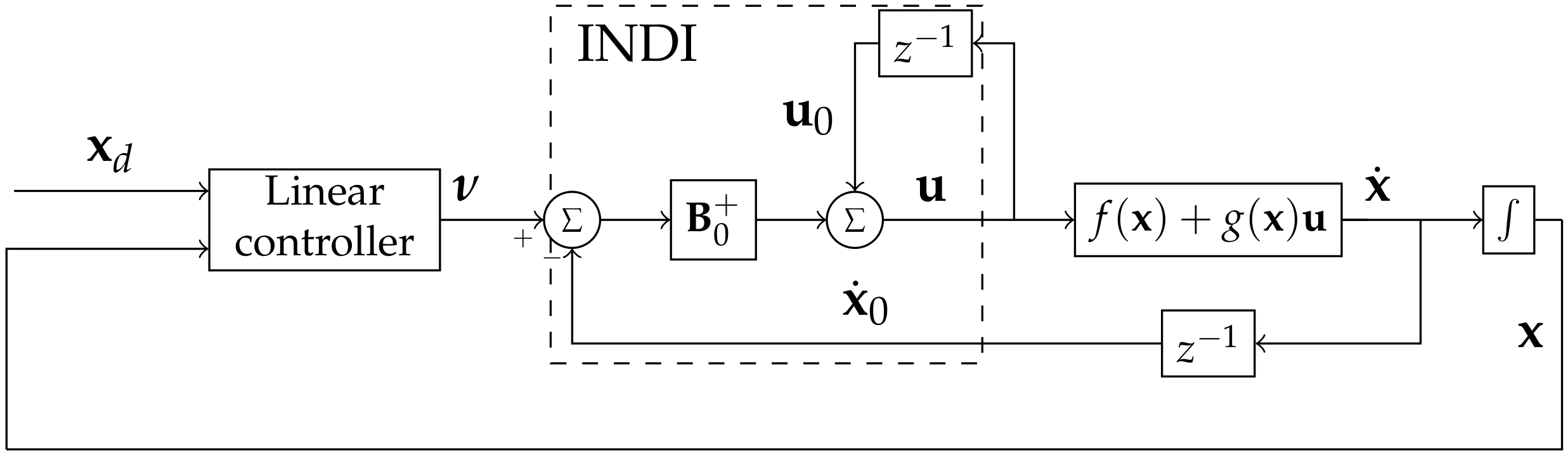
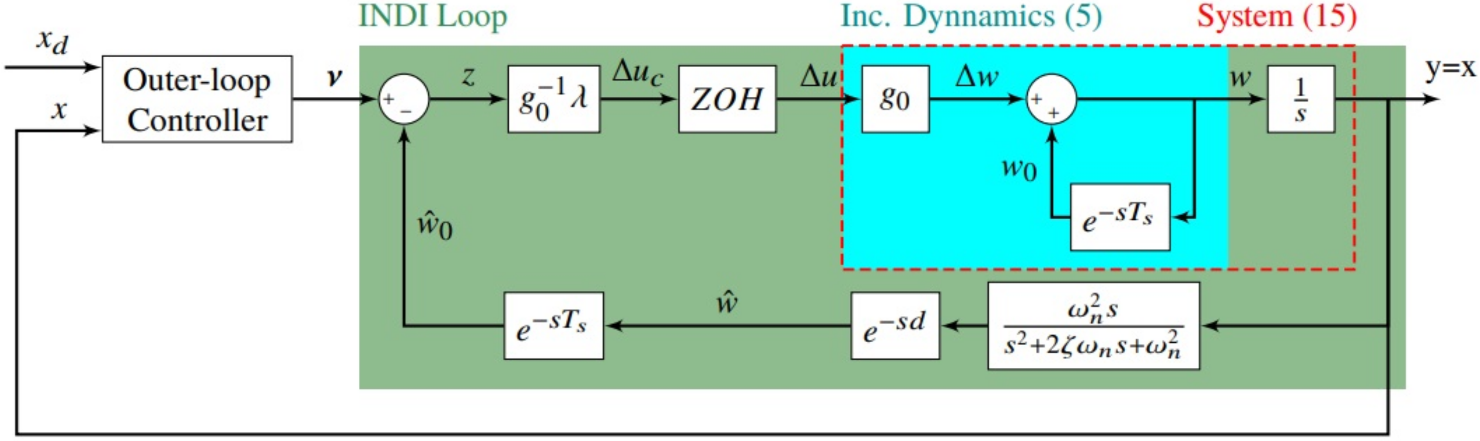
Since all assumptions of Incremental controllers are satisfied we can define the INDI control law (35) for the system in (31a). Figure 7 shows a typical block diagram of a sensor based INDI control, where $z^{-1}$ represents a delay of one sample time.

One of the most important advantages of using incremental controllers, which makes it a successfull candidate for real applications, is the great robustness to model parameters. The most common control approaches are said to be model based, for their design being strongly dependent on the system dynamics model. This aspect requires the definition of an accurate mathematical representation, as well as a careful system identification process. Nevertheless, the resulting model will still be subject to noise, disturbances and remaining model uncertainties.

The approach based on the incremental dynamics on its hand requires only the identification of the input matrix, neglecting the parameters that depend exclusively on the internal states and it is expected to be robust to model uncertainties. Furthermore, the incremental formulation is very simple and intuitive, supported on well established mathematical fundamentals, with only a few parameters to set-up.

On the other hand, restrictions on the use of incremental controllers arise out of assumptions A6.1 to A6.5. Initially, as a consequence of the model simplifications, all the needed information about the system states is obtained from measurements. Thus, to ensure quality in the measurements, the feedback states and state derivatives are to be updated at a sufficiently high sampling rate, with good quality sensors. Furthermore, A6.3 implies that input control signal must have dominance on the system dynamics, demanding fast actuation when compared with system modes. These assumptions are satisfied in the most of UAVs since the control actuation has the greater influence over the dynamics.

In the following subsections we present and analyze the two techniques (WOF and ISG) proposed to mitigate the filtering design problems of input redundancy and second-order filtering delay. The results are illustrated through numerical examples considering an application for the INDI control.

6.2. Input Redundancy Treatment

If we consider that the input matrix ${\mathbf{B}}_0$ from (35) may not be square, we can expect an input redundancy to occur. Therefore, there are various possible solutions of inputs ${\mathbf{u}}_e$ that achieve a given equilibrium point ${\mathbf{x}}_e$. A common issue is that the redundant inputs can cancel each other when the system achieves a stationary state condition, resulting in more energy consumption.

As an example, consider a simplified vehicle dynamics with a single state variable x given by the longitudinal velocity and two inputs $u_1$ and $u_2$. This system dynamics can be represented by the following mathematical modeling:

$$\dot{x}=f\left(x\right)+g_1\left(x\right)u_1+g_2\left(x\right)u_2.$$

(37)

Both control inputs $u_1$ and $u_2$ have influence over the vehicle velocity dynamics. Now consider an equilibrium point $x_e>0$, thus ${\dot{x}}_e=0$ and the following can be stated:

$$\left[\begin{array}{cc}{b}_1& -b_2\end{array}\right]\left[\begin{array}{c}{u}_1\\ u_2\end{array}\right]=-f\left(x_e\right),$$

(38)

where $b_1=g_1\left(x_e\right)$ and $b_2=-g_2\left(x_e\right)$ are positive constants.

In this case, there are many choices for $u_1$ and $u_2$ resulting in the same constant longitudinal velocity $x_e$. However, this choice will impact in the energy consumption. The ideal solution is to use the minimal control effort in order to save energy.

One solution for this problem is to perform a filtering in the commanded redundant input which is less important for maintaining the equilibrium point. As a result we obtain a system dynamics described in the following form:

$$\dot{x}=f\left(x\right)+g_1\left(x\right)u_1+g_2\left(x\right){\widehat{u}}_2,$$

(39a)

$${\dot{\widehat{u}}}_2=\frac{-1}{\tau }{\widehat{u}}_2+u_2.$$

(39b)

where ${\widehat{u}}_2$ is the filtered commanded input for the brake. By imposing this dynamics, $u_2$ will naturally converge to zero and $u_1$ will also reduce, once $u_2$ is no longer canceling it. Note that $u_2$ is still useful for the transient state condition when the vehicle needs to slowdown fast. This strategy is commonly referenced in the literature as Washout Filter (WOF) [13].

The solution can be extended for systems with Multiple Inputs and Multiple Outputs (MIMO). Consider the following generalized MIMO system dynamics:

$$\dot{\mathbf{x}}=f\left(\mathbf{x}\right)+g\left(\mathbf{x}\right)\mathbf{u},$$

(40)

where $\mathbf{x}\in {\mathbb{R}}^n$, $\mathbf{u}\in {\mathbb{R}}^m$ and $m\ge n$.

Thus, applying the WOF to the redundant inputs we obtain the following extended dynamics:

$$\left[\begin{array}{c}\dot{\mathbf{x}}\\ {\dot{\widehat{\mathbf{u}}}}_s\end{array}\right]=\left[\begin{array}{cc}{\mathbf{I}}_n& g_s\left(\mathbf{x}\right)\\ {\mathbf{0}}_{l\times n}& {\mathbf{T}}_s\end{array}\right]\left[\begin{array}{c}f\left(\mathbf{x}\right)\\ {\widehat{\mathbf{u}}}_s\end{array}\right]+\left[\begin{array}{cc}{g}_m\left(\mathbf{x}\right)& {\mathbf{0}}_{n\times l}\\ {\mathbf{0}}_{l\times n}& {\mathbf{I}}_l\end{array}\right]\left[\begin{array}{c}{\mathbf{u}}_m\\ {\mathbf{u}}_s\end{array}\right]$$

(41)

where: $l=m-n$, $\mathbf{x}\in {\mathbb{R}}^n$ is the vector of states; ${\mathbf{u}}_m\in {\mathbb{R}}^n$ is the vector of main actuators; ${\mathbf{u}}_s\in {\mathbb{R}}^l$ is the vector of secondary (or redundant) actuators; ${\widehat{\mathbf{u}}}_s\in {\mathbb{R}}^l$ is the vector of filtered input signals, $f\left(\mathbf{x}\right)$ is the function of state dynamics; $g_m\left(\mathbf{x}\right)$ is a function which describes the influence of ${\mathbf{u}}_m$ in the state dynamics; $g_s\left(\mathbf{x}\right)$ is a function which describes the influence of ${\mathbf{u}}_s$ in the state dynamics; ${\mathbf{T}}_r=\mathrm{diag}\left([-1/{\tau }_1;-1/{\tau }_2;-1/{\tau }_3;\cdots ;-1/{\tau }_l]\right)$ is a diagonal matrix with positive constants ${\tau }_1,\cdots ,{\tau }_l$ chosen by the designer; ${\mathbf{I}}_n$ is the identity matrix of order n; and ${\mathbf{0}}_{n\times l}$ is a matrix full of zeros with n lines and l columns.

The vector of redundant actuators can be chosen by analyzing the input function $g\left(\mathbf{x}\right)$ through a systematic procedure. First, the designer must linearize $g\left(\mathbf{x}\right)$ in a chosen point ${\mathbf{x}}_0$, obtaining the following:

$${\mathbf{B}}_0=\frac{\partial }{\partial \mathbf{x}}g\left(\mathbf{x}\right){|}_{x_0}.$$

(42)

By analyzing the matrix ${\mathbf{B}}_0\in {\mathbb{R}}^{n\times m}$, the designer must identify the linearly dependent columns, which indicates the redundant inputs. After identifying the redundant actuators, the designer must choose and separate between main (${\mathbf{u}}_m$) and secondary (${\mathbf{u}}_s$) actuators, by also defining the functions $g_m\left(\mathbf{x}\right)$ and $g_s\left(\mathbf{x}\right)$. 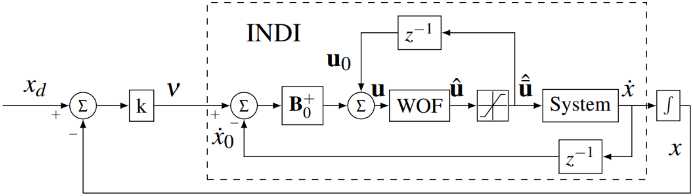Then the extended dynamics (41) can be applied. This solution can be represented by a block diagram in a cascaded form as shown in Figure 8, where $\widehat{\mathbf{u}}={\left[{\mathbf{u}}_m{\widehat{\mathbf{u}}}_s\right]}^T$ and $g\left(\mathbf{x}\right)=\left[g_m\left(\mathbf{x}\right)g_s\left(\mathbf{x}\right)\right]$.

Numerical Example

As an example consider the following linear system with two redundant inputs:

$$\dot{x}=x+0.2u_1-0.8u_2$$

(43)

where x is the state, $u_1$ is the first input and $u_2$ is the second input.

By applying INDI, we obtain the following control law:

$$\mathbf{u}={\mathbf{u}}_0+{\mathbf{B}}_0^{+}(\nu -{\dot{x}}_0)$$

(44)

where $\mathbf{u}={\left[u_1{u}_2\right]}^T$, ${\mathbf{B}}_0=[0.2-0.8]$, ${\mathbf{u}}_0$ is the previous input and $\nu =k(x_d-x)$ is a desired dynamics of first order. The block diagram in Figure 8 illustrates the closed loop system, where $z^{-1}$ represents a delay of one sample time $t_s=0.01$ seconds, $\widehat{\mathbf{u}}={\left[u_1{\widehat{u}}_2\right]}^T$ is the control signal filtered by the WOF, $k=20s^{-1}$ is a linear gain and $\tau =5$ seconds is the time constant of the WOF. We suppose the presence of actuator saturation ($-0.5\le u_1\le 0.5$ and $-0.5\le u_2\le 0.5$,) which is treated with an anti-windup strategy [3].

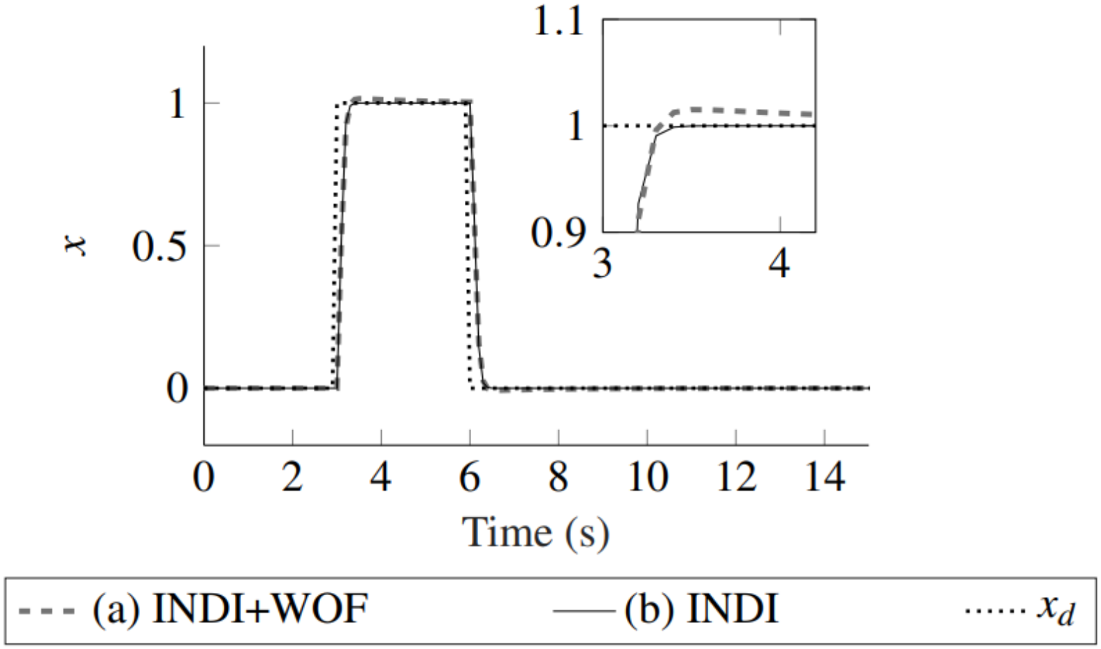
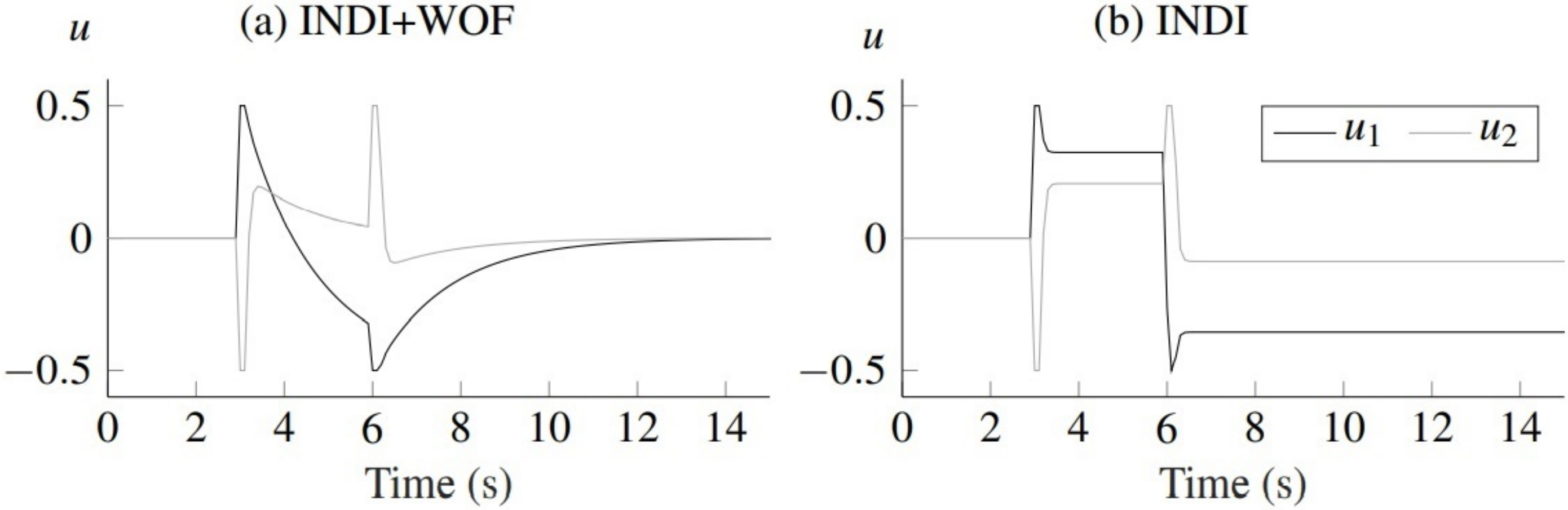
Figure 9 and Figure 10 show the results for a step in $x_d$ using WOF denominated case (a) (or “INDI+WOF”) and without WOF denominated case (b) (or “INDI”). For sake of comparison consider the following quadratic cost function:

$$J_u={\int }_0^{t_f}{u}_1^2\left(t\right)+u_2^2\left(t\right)dt$$

(45)

where $t_f=15$ seconds is the final time of simulation.

From the figures, we see that the tracking performance is similar for both cases, which does not happen for the control effort. In Figure 10, the saturation is achieved in both control inputs for both cases (a) and (b). In case (b) the commanded signals $u_1$ and $u_2$ converge to values different from zero after the transient state ($t>6$ seconds). Consequently the system has higher energy consumption in case (b) with $J_u=17.85$. In case (a) the energy consumption is reduced to $J_u=5.74$. Therefore, the WOF appears as a simple and advantageous solution for systems with redundant actuation with actuator saturation, such as aerial vehicles i.e. multirotor drones, aircrafts and airships.

6.3. The Second-Order Differentiator and the Estimation of Derivatives

One important problem in control design, not limited to incremental controllers, is the need for the derivative of a given state. They may be difficult to obtain or even impossible, as is the case of the derivative of angular rates. Further, direct numerical differentiation of the output signal may lead to noise amplification and abrupt variations.

A common solution to this problem is the use a Second-Order Differentiator (SOD) to obtain the derivative of the state. The SOD works as a low-pass filter for the state yielding a filtered output of the measure $\mathbf{y}$. While providing an estimation of the state derivative, the SOD simultaneously attenuates the high-frequency noise in the measure signal.

If we call the state derivative vector as $\mathbf{w}=\dot{\mathbf{x}}$, the estimation of the derivative $\widehat{\mathbf{w}}$, using the second-order-derivative (SOD), is given by:

$$\widehat{\mathbf{w}}\left(s\right)=\left[\frac{{\omega }_n^{2}s}{s^2+2\zeta {\omega }_{n}s+{\omega }_n^2}\right]\mathbf{y}\left(s\right).$$

(46)

In the design procedure, the filter parameters like the natural frequency ${\omega }_n$ and the damping ratio $\zeta$ are used to adjust the passband mid-frequency, as well as the passband size.

6.4. Input Scaling Gain

A drawback that comes with the SOD filter is the natural delay produced by the second order dynamics, which may harm the control system feedback. Thus, it is important to mitigate this delayed estimation in order to robustify the controller.

One possible solution to this issue is the so called Input Scaling Gain (ISG), that was first proposed by our research group in 2015 [14], as a scalar factor. In this paper, we propose the generalization of the scale gain to MIMO systems, using a diagonal matrix $\mathbf{\Lambda }\in {\mathbb{R}}^{n\times n}$. In the case of the incremental controller design, the ISG is used to scale down the difference $(\nu -{\dot{\mathbf{x}}}_0)$ in (35), reducing the bandwidth of the closed-loop system. The matrix diagonal elements ${\lambda }_{ii}$ are real numbers in the interval $[0,1]$, such that the modified INDI control law is now given as:

$$\mathbf{u}={\mathbf{u}}_0+{\mathbf{B}}_0^{+}\mathbf{\Lambda }(\nu -{\dot{\mathbf{x}}}_0),$$

(47)

Note that with $\mathsf{\Lambda }={\mathbf{I}}_n$ we have the traditional INDI control law (35).

Substituting (47) in the closed loop Incremental Dynamics (34) results in:

$$\dot{\mathbf{x}}={\dot{\mathbf{x}}}_0+\mathbf{\Lambda }(\nu -{\dot{\mathbf{x}}}_0).$$

(48)

Considering the discrete implementation, where the time interval between $t_0$ and t is $\Delta t=T_s$, we can rewrite (48) as:

$$\frac{\Delta \dot{\mathbf{x}}}{\Delta t}=\frac{\Delta \dot{\mathbf{x}}}{T_s}=\frac{1}{T_s}\mathbf{\Lambda }(\nu -{\dot{\mathbf{x}}}_0),$$

(49)

Assuming a fast sampling rate (small $\Delta t$), and denoting $\dot{\mathbf{x}}$ as $\mathbf{w}$, (49) approximates to:

$$\dot{\mathbf{w}}\simeq \frac{1}{T_s}\mathbf{\Lambda }(\nu -{\mathbf{w}}_0).$$

(50)

Considering $t_0=t-T_s$, (50) can be rewritten as:

$$\dot{\mathbf{w}}\left(t\right)=\frac{1}{T_s}\mathbf{\Lambda }\left[\nu \left(t\right)-\mathbf{w}(t-T_s)\right].$$

(51)

Applying Laplace transform to (51), provides the transfer function between the state derivative and the pseudo-control as:

$$\begin{array}{c}\mathcal{L}\left\{\dot{\mathbf{w}}\left(t\right)+\frac{1}{T_s}\mathbf{\Lambda }\mathbf{w}(t-T_s)\right\}=\frac{1}{T_s}\mathbf{\Lambda }\mathcal{L}\left\{\nu \left(t\right)\right\}\iff \\ \iff T_s{\mathbf{\Lambda }}^{-1}s\mathbf{w}\left(s\right)+e^{-s{T}_s}\mathbf{w}\left(s\right)=\nu \left(s\right)\iff \\ \iff \mathbf{w}\left(s\right)={\left(T_s{\mathbf{\Lambda }}^{-1}s+e^{-s{T}_s}\mathbf{I}\right)}^{-1}\nu \left(s\right)=\mathrm{diag}\left\{\frac{1}{\frac{T_s}{{\lambda }_{ii}}s+e^{-s{T}_s}}\right\}\nu \left(s\right).\end{array}$$

(52)

Some important points to be remarked are:

• each component of ${\nu }_i$ of pseudo-control $\nu$ has an independent time constant $\frac{T_s}{{\lambda }_{ii}}$, as the scale matrix $\mathbf{\Lambda }$ is a diagonal matrix.
• Under fast sampling, we can assume $e^{-s{T}_s}\simeq 1$ implying that (52) simplifies to a simple first order low-pass filter, attenuating high-frequency perturbations in the pseudo-control $\nu$;
• as a possible drawback, the ISG reduces the bandwidth of the closed-loop dynamics, eventually decreasing the overall performance;

6.5. Combining ISG and SOD: Closed-Loop Analysis

In order to investigate the stability properties as well as the performance improvements against delays in the closed-loop system, we analyze here the proposed SOD+ISG solution for a first-order SISO system, as shown in Figure 11.

Although illustrated here for a SISO system, the approach can be extended to multiple-input-multiple-output (MIMO) systems as the diagonal structure of the ISG yields independent components $z_i$ of the INDI-loop error $\mathbf{z}=\nu -{\mathbf{w}}_0$, and the SOD is also independent for each state $x_i$.

Firstly, to consider continuous systems, the discrete sample delays $z^{-1}$ of INDI (see Figure 7) are substituted by time delay components $e^{-s{T}_s}$. Further, to simulate the discrete feature of INDI we add a Zero-Order Hold (ZOH) in the control loop, as well as an extra transport delay d to investigate the effects of additional unmodeled delays in the loop.

6.5.1. Analytical Formulation

The system to be controlled is defined as:

$$\left\{\begin{array}{c}\hfill \dot{x}={\dot{x}}_0+g\left(x_0\right)\Delta u\hfill \\ \hfill y=x\hfill \end{array}\right.,$$

(53)

where its dynamics is described using ID formulation (34), and its output is the state itself.

In this section we only analyze the local behavior of the system, where the control effectiveness function $g\left(x_0\right)$ is approximated by a constant $g_0$.

The transfer function $H_1\left(s\right)$ relating the state derivative w with the input increment $\Delta u$ is given (34) by:

$$H_1\left(s\right)=\frac{w\left(s\right)}{\Delta u\left(s\right)}=g_0\left(\frac{1}{1-e^{-s{T}_s}}\right),$$

(54)

and, thus, the transfer function $H_2\left(s\right)$ is given (53) by:

$$H_2\left(s\right)=\frac{y\left(s\right)}{\Delta u\left(s\right)}=\frac{1}{s}{H}_1\left(s\right).$$

(55)

One important feature of the INDI controller, as shown in (36), is that the state derivative w should follow a given pseudo-control $\nu$. Therefore, it is important to analyze the transfer function from $\nu$ to w, denoted here as $H_3\left(s\right)$, shown in the block diagram of Figure 11, and given by:

$$\begin{array}{cc}\hfill H_3\left(s\right)=\frac{w\left(s\right)}{\nu \left(s\right)}& =\frac{g_0^{-1}\lambda Z\left(s\right)H_1\left(s\right)}{1+g_0^{-1}\lambda Z\left(s\right)H_2\left(s\right)\frac{{\omega }_n^{2}s}{s^2+2\zeta {\omega }_{n}s+{\omega }_n^2}{e}^{-s(T_s+d)}}\hfill \\ \hfill & =\frac{g_0^{-1}\lambda Z\left(s\right)H_1\left(s\right)\left(s^2+2\zeta {\omega }_{n}s+{\omega }_n^2\right)}{s^2+2\zeta {\omega }_{n}s+{\omega }_n^2+g_0^{-1}\lambda {\omega }_n^2{e}^{-s(T_s+d)}Z\left(s\right)H_2\left(s\right)s},\hfill \end{array}$$

(56)

where $Z\left(s\right)=\frac{1-e^{-s{T}_s}}{s{T}_s}$ is the zero-order-holder.

Substituting (54), (55), and $Z\left(s\right)$ into (56), we finally come to the transfer function from $\nu$ to w as:

$$H_3\left(s\right)=\frac{\frac{\lambda }{T_s}\left(s^2+2\zeta {\omega }_{n}s+{\omega }_n^2\right)}{s^3+2\zeta {\omega }_n{s}^2+{\omega }_n^{2}s+\frac{\lambda }{T_s}{\omega }_n^2{e}^{-s(T_s+d)}}.$$

(57)

Note that (57) is a delayed system where the delay appears in the constant term of the characteristic equation, such that the simple first-order Padé approximation

$$e^{-sT}\approx \frac{1-sT/2}{1+sT/2}.$$

(58)

can be used to investigate the stability analysis of the closed-loop system.

The resulting transfer function $H_3\left(s\right)$ is finally approximated to:

$$H_3\left(s\right)=\frac{\frac{\lambda }{T_s}\left(1+s\frac{(T_s+d)}{2}\right)\left(s^2+2\zeta {\omega }_{n}s+{\omega }_n^2\right)}{\frac{(T_s+d)}{2}{s}^4+\left(\zeta {\omega }_n(T_s+d)+1\right)s^3+\left(2\zeta {\omega }_n+\frac{(T_s+d)}{2}{\omega }_n^2\right)s^2+\left(\frac{(2-\lambda )T_s-\lambda d}{2T_s}{\omega }_n^2\right)s+\frac{\lambda }{T_s}{\omega }_n^2}.$$

(59)

From which we can conclude that:

• As desired in the INDI approach, w will follow a pseudo control $\nu$, due to the fact that the transfer function has unitary dc-gain;
• Considering the Routh–Hurwitz criterion, $H_3\left(s\right)$ will be stable for positive coefficients in the characteristic polynomial, which implies that $(2-\lambda )T_s-\lambda d>0$;
• Further, the ISG is also effective to mitigate the effects of additional delays in the closed-loop. For example, without the use of ISG ($\lambda =1$), the extra delay should never be greater than the sample time $T_s$.

6.5.2. Numerical Example

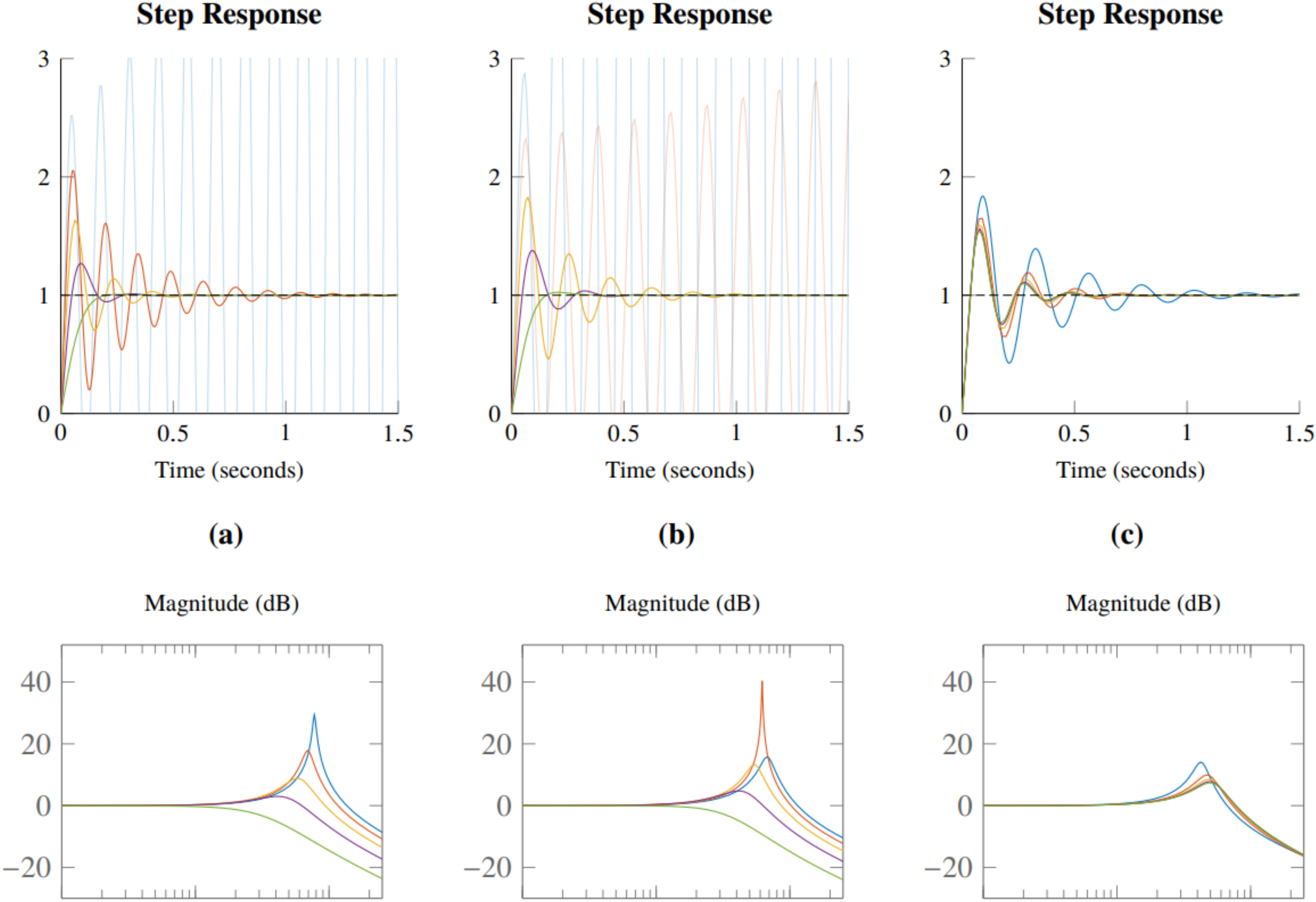
A numerical example is presented here to investigate the effect of the ISG gain and the SOD differentiator approach in the control loop. To investigate the role of the delay in the INDI control, let us analyze the scenario in which there is an extra delay $d>T_s$ in the INDI feedback loop. Figure 12 shows the results for the step inputs applied to $H_3\left(s\right)$ and the corresponding Bode plots, assuming a sampling frequency of 50 Hertz.

The simulations were done for three diferent conditions: a) Varying ISG scale gains for a given measured state derivative (note that lower $\lambda$ implies lower natural frequency and bigger damping ratio); b) Varying ISG scale gains for a differentiator with a given natural frequency of $\frac{15}{T_s}$; and c) Varying the natural frequencies of the differentiators for a fixed ISG gain equal to 0.5.

The step response plots, without using the ISG (equivalent to $\lambda =1$), shows that the system is unstable for this plant that has an extra delay d larger than the sample time $T_s$. However, the system becomes stable if a lower value of $\lambda$ is considered. For the case where the bandwidth of the differentiator satisfies the relation ${\omega }_n{T}_s=15$, the extra delay d added by the filter destabilizes the system even if we use an ISG gain of 0.8, while an ISG gain of 0.5 is sufficient to make it stable for different SOD frequencies.

From these results, we conclude that the combined approach SOD + ISG yields a useful and practical derivative estimator, since the ISG can mitigate the effects of the delay generated by the second-order differentiator. Additionally, we remark that it can even mitigate other possible delays appearing in the feedback loop.

7. Conclusions

In this paper we presented a comparative study evaluating different solutions for the state estimation of a robotic airship as well as its derivatives. For the state estimation we used a second order filter, an Extended Kalman Filter and an Unscented Kalman Filter. We performed all simulations using a high-fidelity airship dynamic model for Simulink platform. For the state estimation, the EKF showed a better performance when compared to the other estimation techniques.

In a second moment, we presented a Model-based (EKF) and a Data-driven (Neural Network) approaches for the estimation of the wind velocity. Also, we proposed a novel Hybrid approach, by performing a fusion between the designed Model-based and Data-driven approaches in a cascaded structure. While the NN approach alone tends to estimate the wind speed with an offset (bias), the EKF estimation has long delays for sudden wind changes. However, the Hybrid approach tends to yield a faster response with small bias for the estimated wind components.

Finally, we presented possible solutions to mitigate two common problems arriving in control implementation that are the control input redundancy and the delay introduced by second-order filters. The first one is solved with the use of the Wash Out Filter (WOF). The second one is mitigated with the use of the Input Scaling Gain (ISG) which is generalized here for the MIMO case. To illustrate the design solutions we applied the techniques for the design of incremental controllers, although they can be used also for other nonlinear control approaches in the same situation.