
Study of the Impact of Traffic Flows on the ATC Actions

 , , ,
, , ,
Abstract
:1. Introduction
1.1. Background and Related Work
1.2. Focus and Structure of the Document
2. Materials and Methods
2.1. Data
2.1.1. Flow Data
2.1.2. Traffic Data
2.1.3. Atom Data
2.2. Machine Learning
- Supervised learning: In supervised learning, the training data that are fed into the algorithm include the desired solutions, called labels. In this case, the label will be related to the workload that a flight causes to the controller. This type of model has been chosen because the feature to be predicted is known in advance. A typical supervised learning task is classification. Flights are divided into two groups according to the actions received, and the model learns to classify a flight into one or the other. Another typical task is to predict a target numerical value, given a set of features called predictors. This type of task is called regression. In this case, the model tries to predict the number of actions a flight has received from the controller given a set of features. Supervised learning has proven to work well for solving both classification and regression problems in the ATM field [15,16].
- Batch learning: In batch learning, the system does not learn incrementally, it is trained using all available data. First the system is trained, then it goes into production and runs without learning more; it only applies what it has learned. This is called offline learning. In order for a batch learning system to learn new data, a new version of the system has to be trained from scratch on the complete dataset (not only the new data, but also the old data). This is the type of system chosen, since it is based on initial data and there will not be a regular arrival of new data. In the context of a real use of the models studied in the work, an online system would be necessary. The system would continue to learn and adapt continuously with the new data generated every day.
- Model-based learning: The aim is to generalise from a set of examples to build a model. This model is then used to make predictions. Other works have recently used this approach in the field of ATM, using machine learning to develop new mathematical models to determine air traffic complexity [17].
2.3. Machine Learning Algorithms
2.3.1. Decision Trees
2.3.2. Random Forest
2.3.3. XGBoost
- Random forests build each tree independently, while gradient boosting builds one tree at a time. This additive model works incrementally, introducing a weak learner to improve the deficiencies of existing weak learners;
- Random forests combine the results at the end of the process by averaging, while gradient boosting combines the results throughout the process.
2.4. Explainability Methods
2.4.1. ELI5
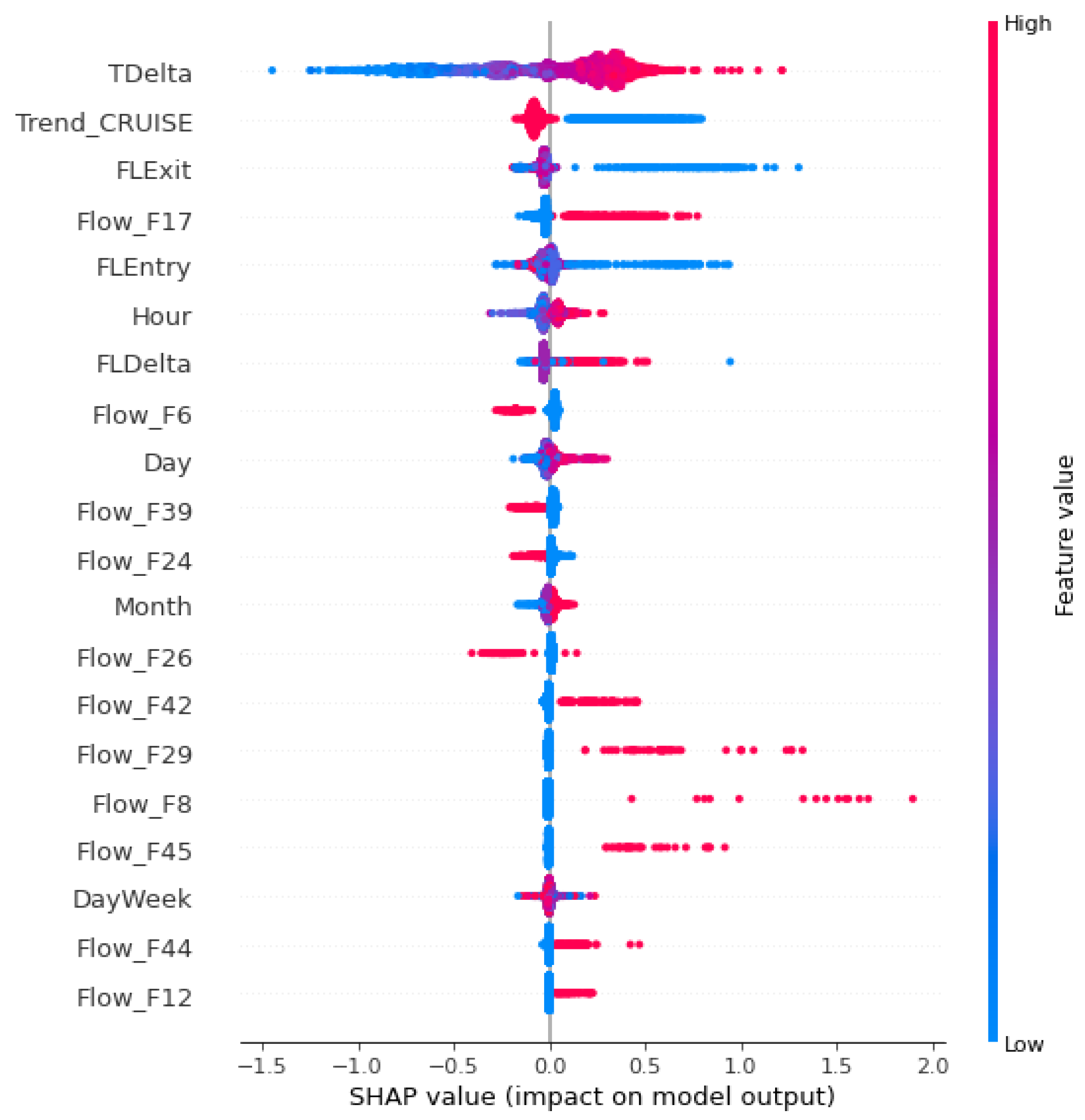
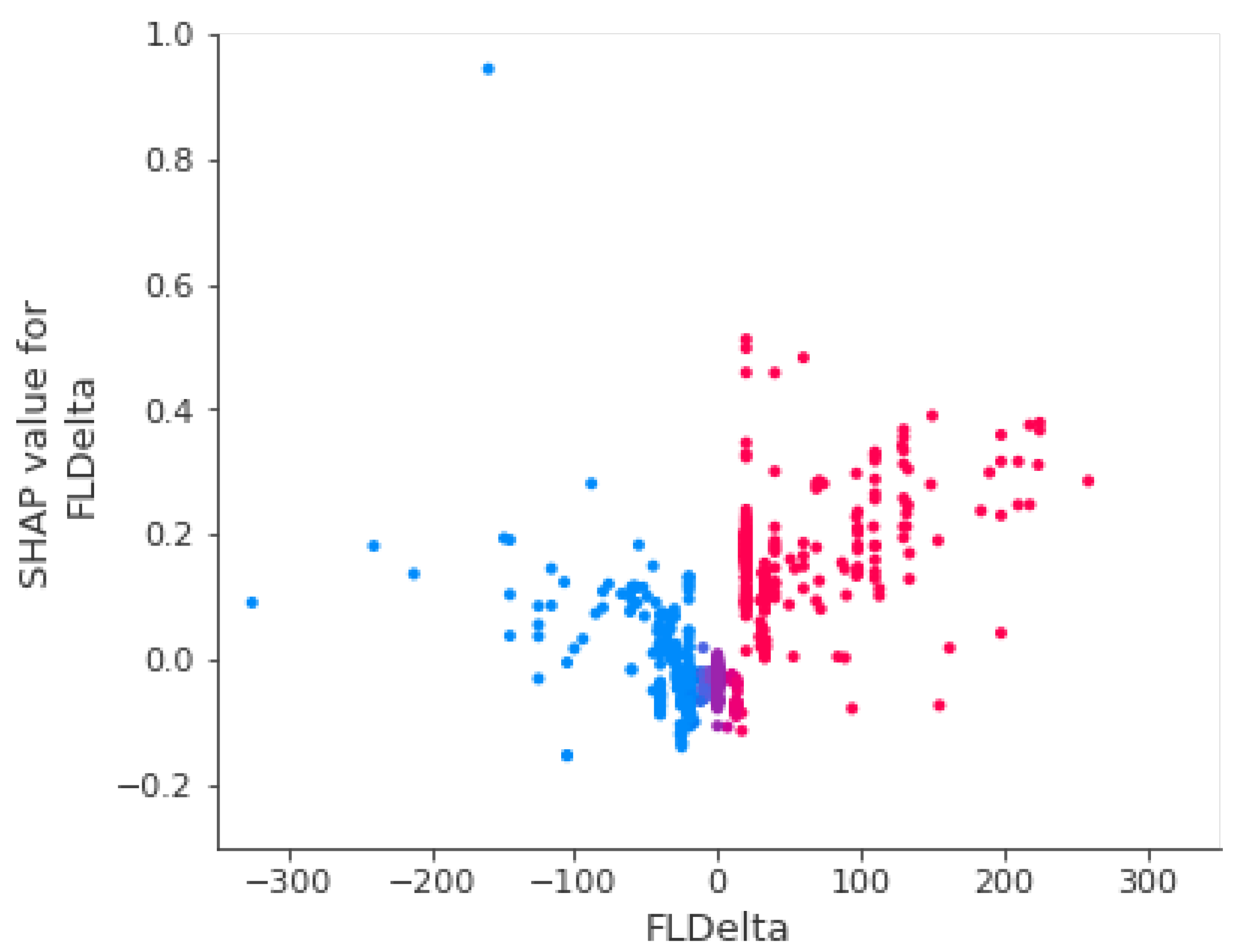
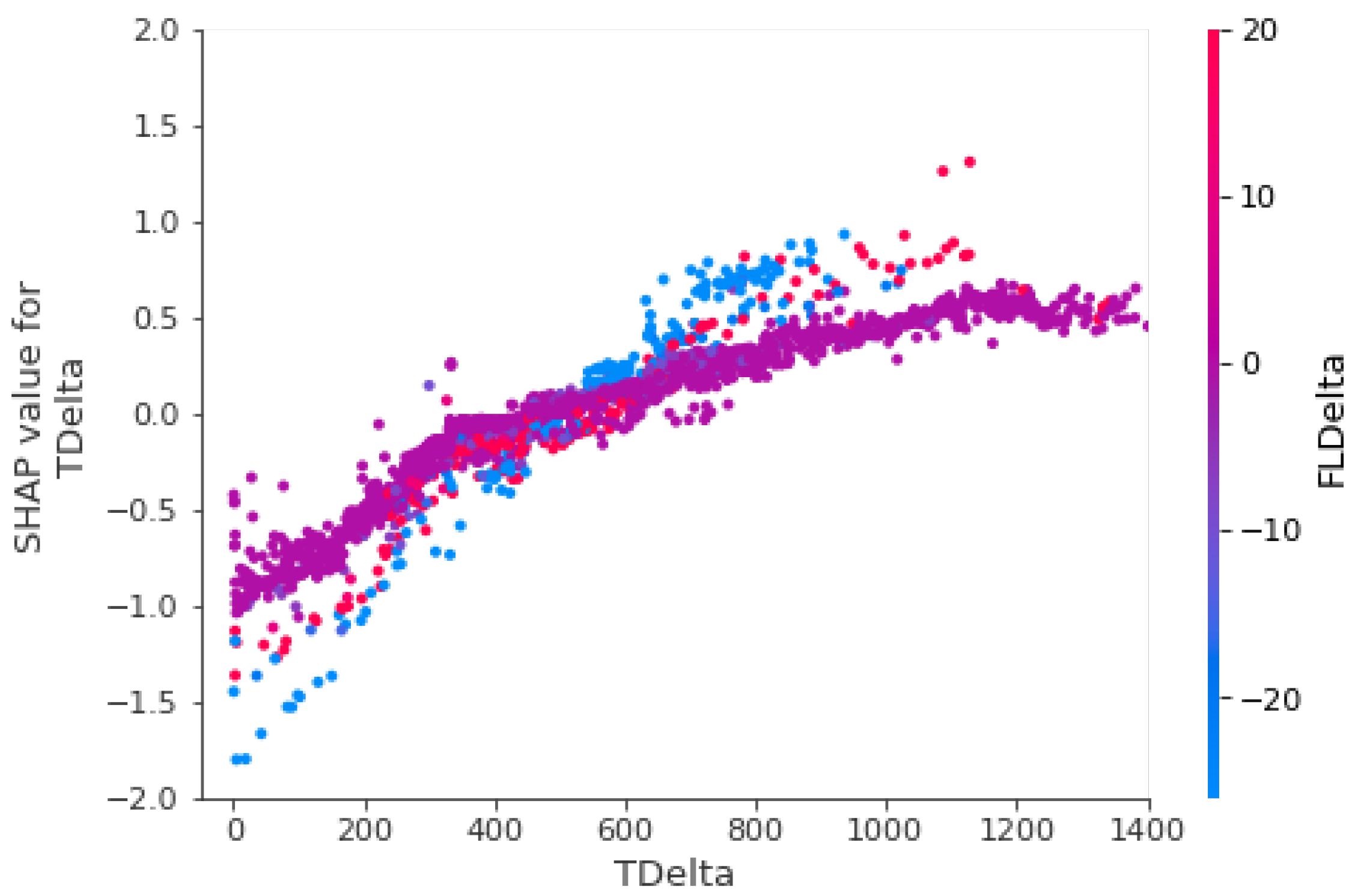
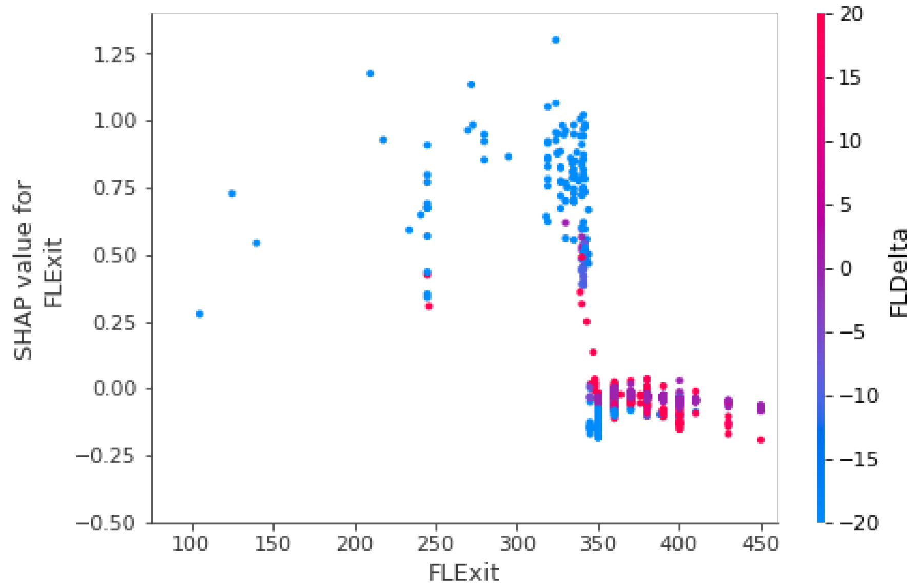
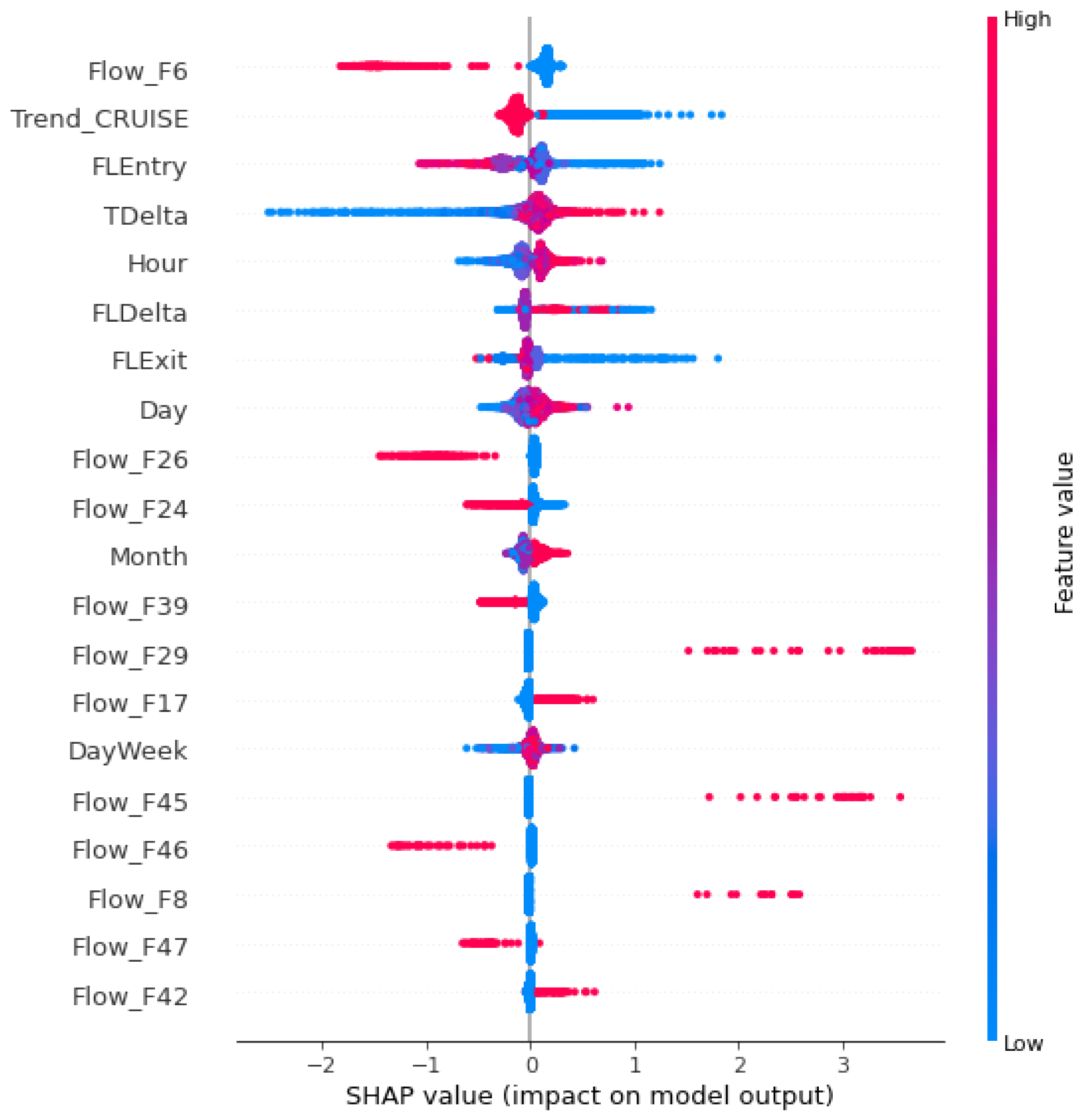
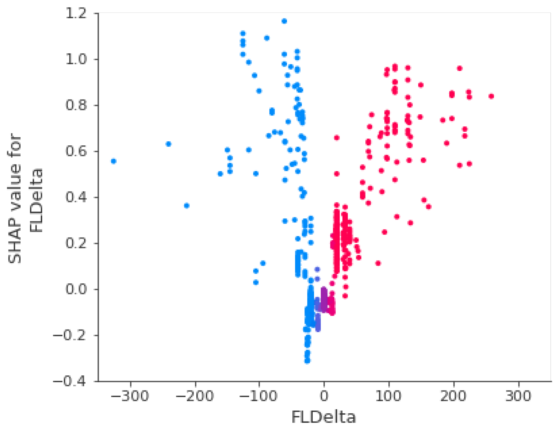
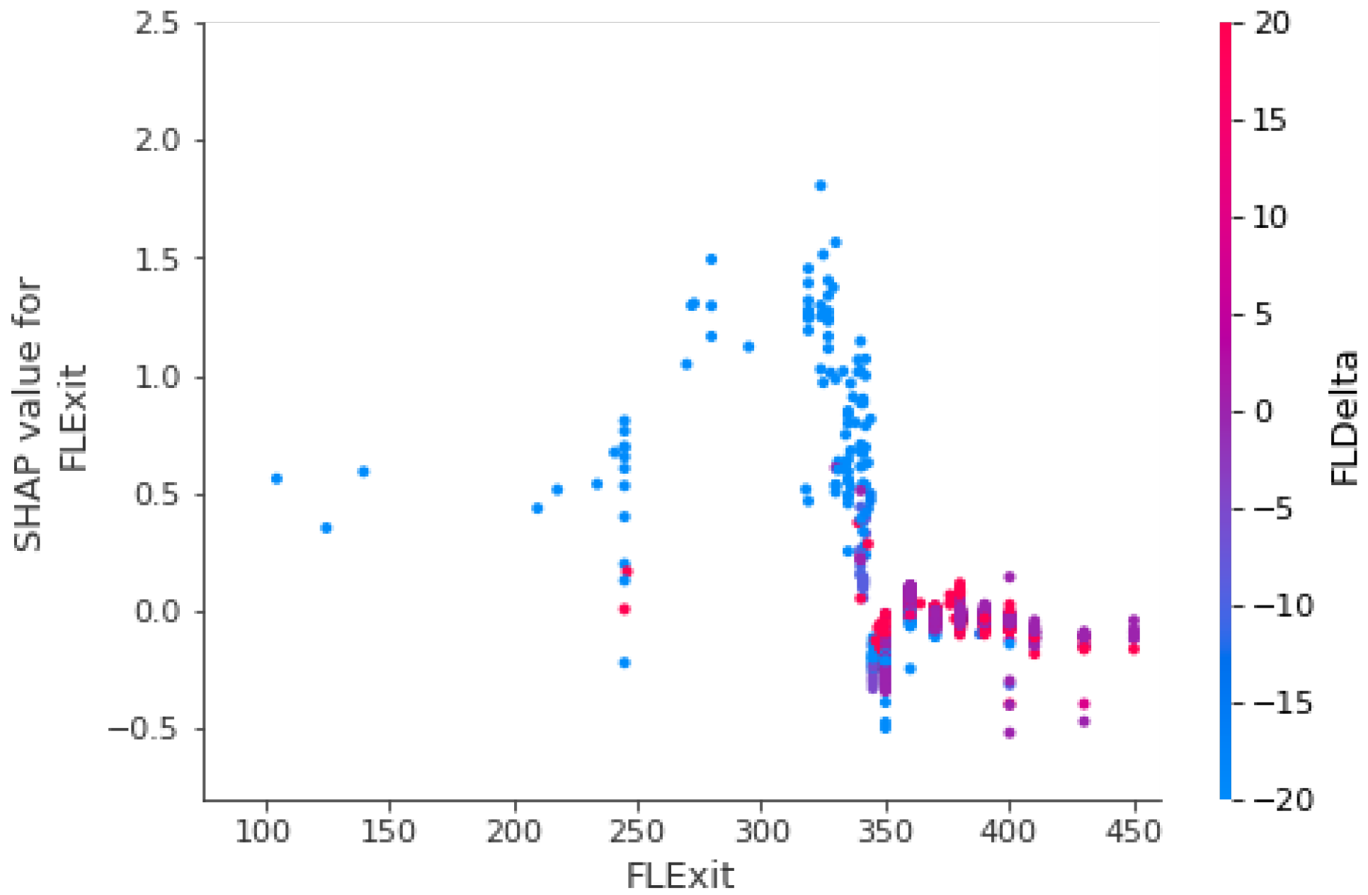
2.4.2. SHAP (Shapley Additive Explanations)
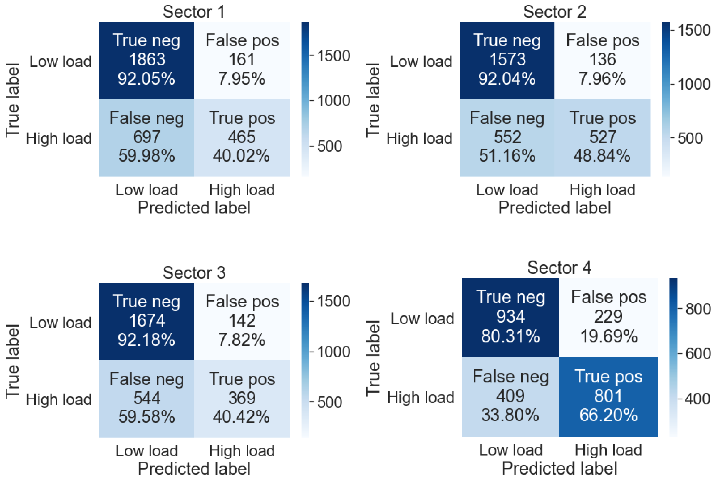
2.4.3. Confusion Matrix
3. Results
3.1. Exploratory Data Analysis
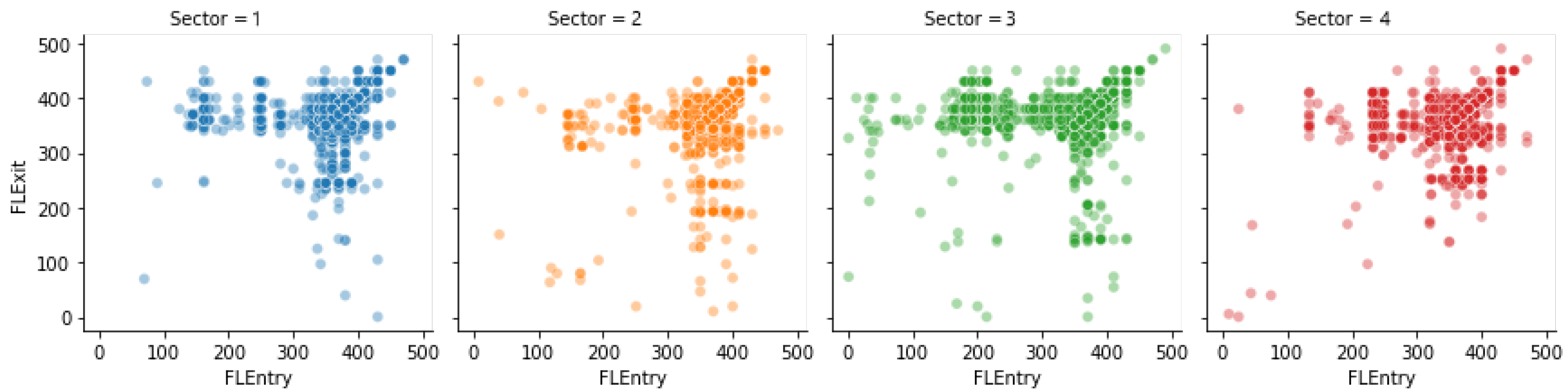
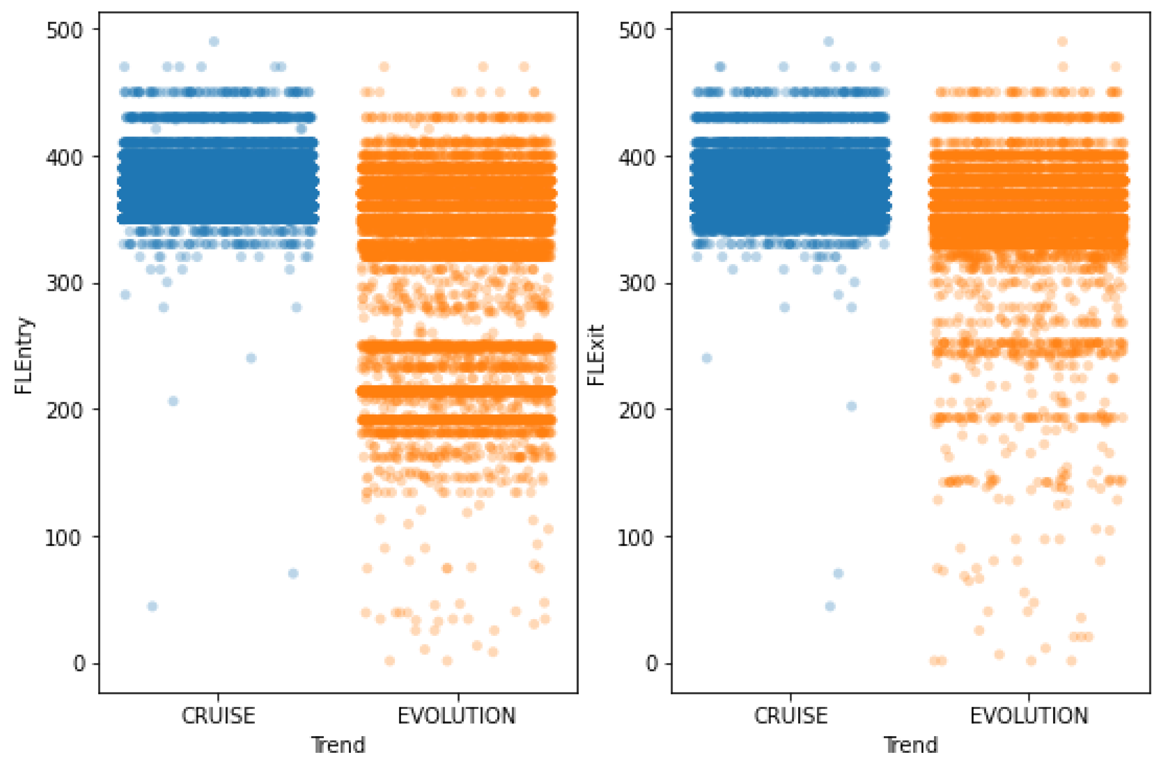
3.1.1. Flight Levels
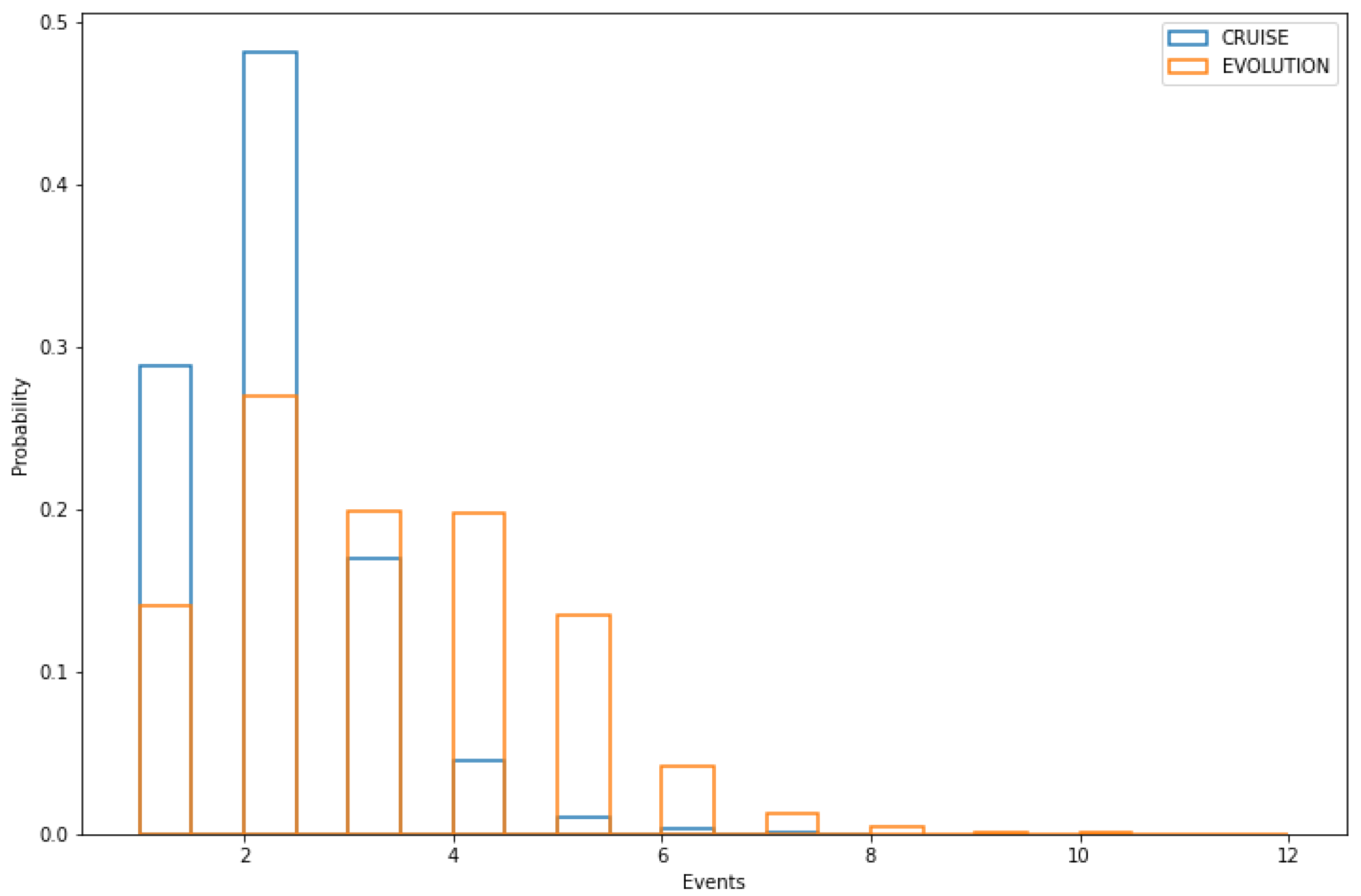
3.1.2. Events
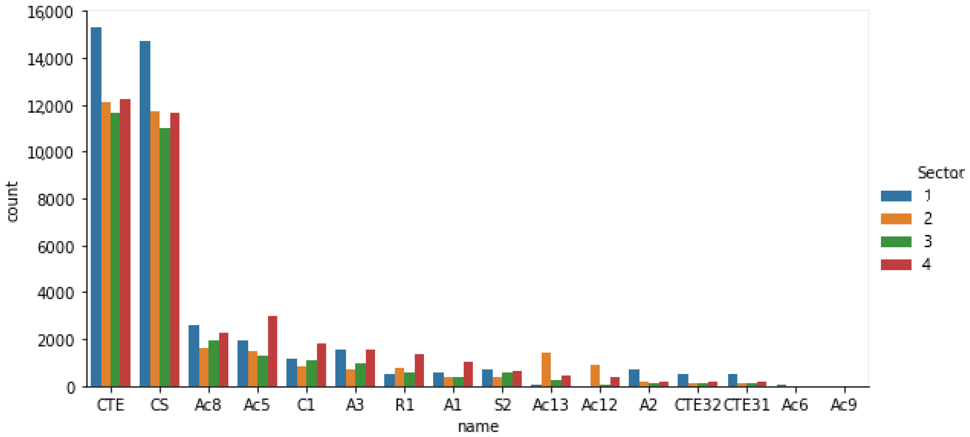
3.1.3. ATCo Actions
3.2. Feature Engineering
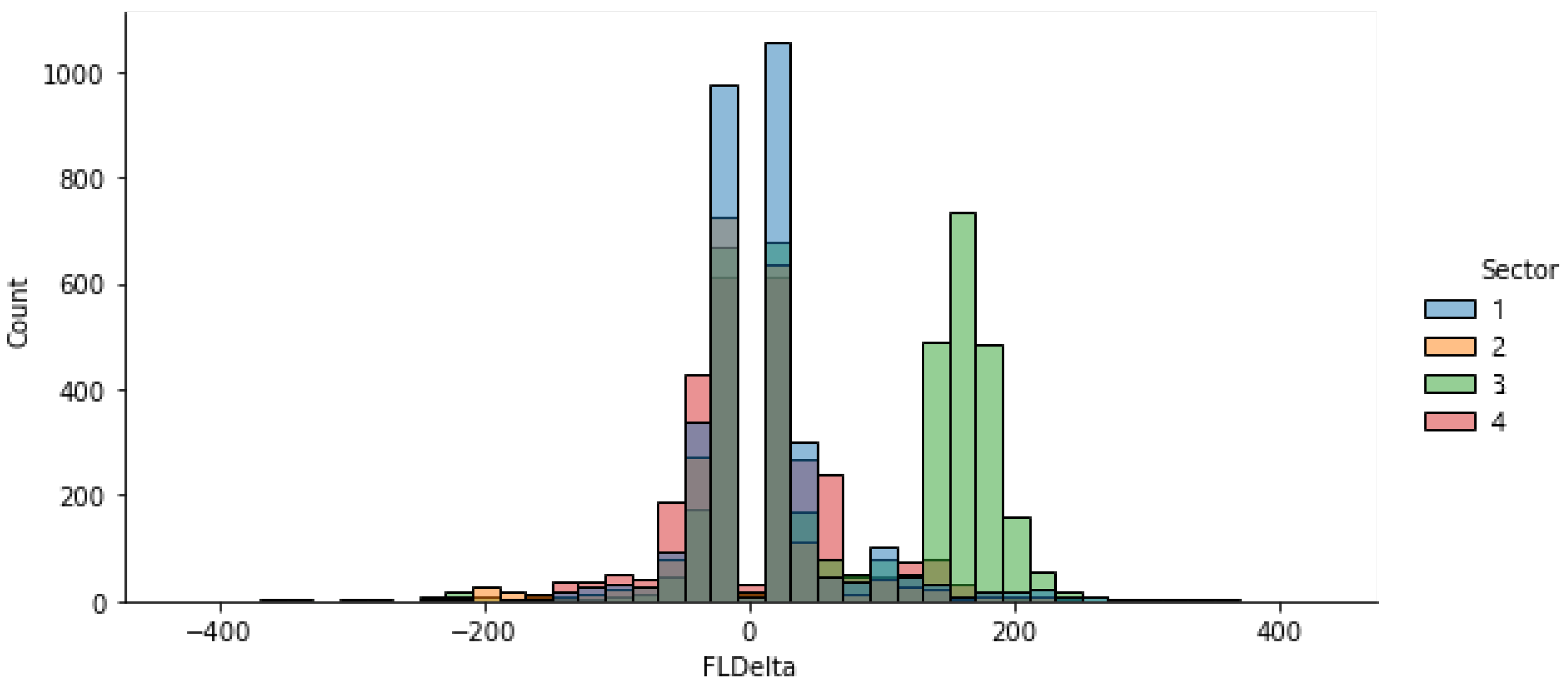
3.2.1. FLDelta
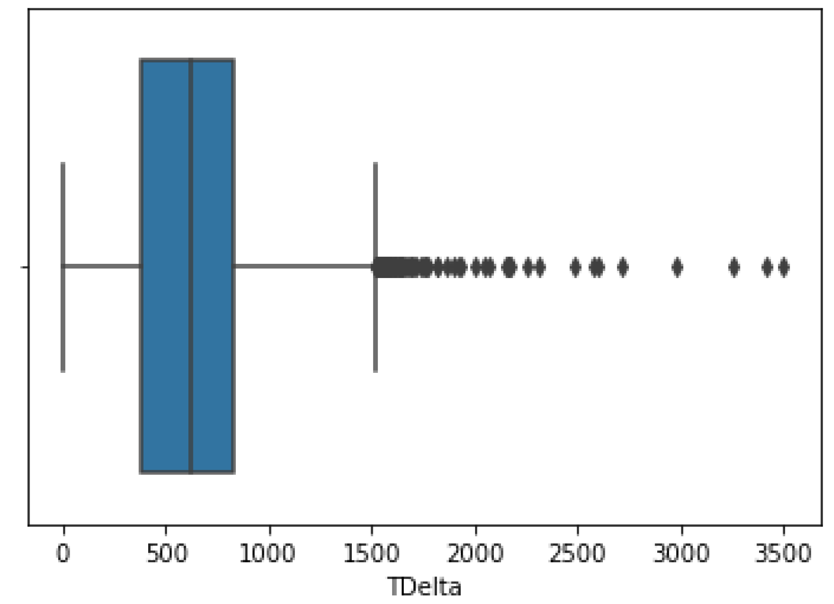
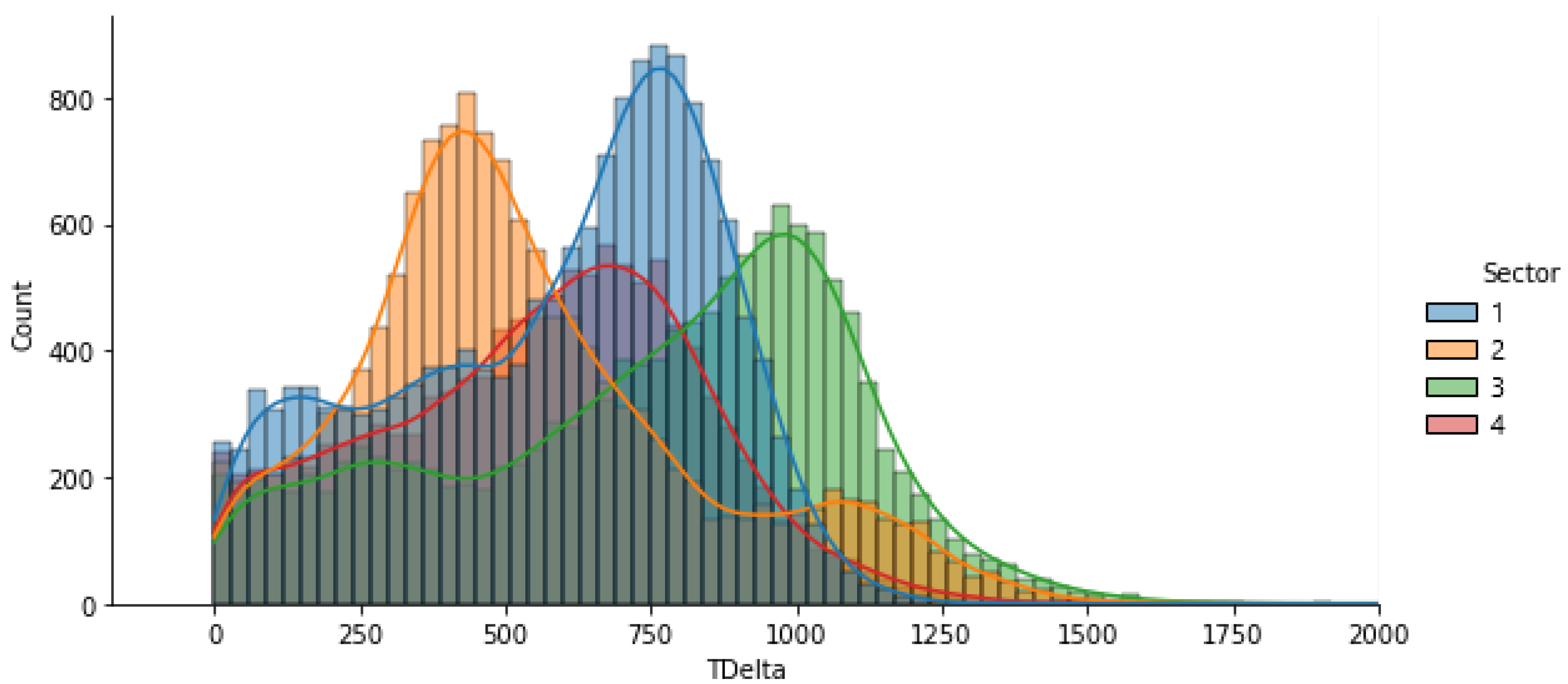
3.2.2. TDelta
3.3. Machine Learning Models
3.4. Results of Selected Models
3.4.1. Regression Model
3.4.2. Classification Model
3.4.3. General Approach
4. Conclusions and Future Lines of Research
4.1. Conclusions
4.2. Future Lines of Research
Author Contributions
Funding
Institutional Review Board Statement
Informed Consent Statement
Data Availability Statement
Conflicts of Interest
References
- Wang, Y.; Hu, R.; Lin, S.; Schultz, M.; Delahaye, D. The Impact of Automation on Air Traffic Controller’s Behaviors. Aerospace 2021, 8, 260. [Google Scholar] [CrossRef]
- Metzger, U.; Parasuraman, R. Automation in future air traffic management: Effects of decision aid reliability on controller performance and mental workload. In Decision Making in Aviation; Routledge: Oxfordshire, UK, 2017; pp. 345–360. [Google Scholar]
- Rodríguez, S.; Sánchez, L.; López, P.; Cañas, J.J. Pupillometry to Assess Air Traffic Controller Workload through the Mental Workload Model. In Proceedings of the 5th International Conference on Application and Theory of Automation in Command and Control Systems (ATACCS ’15), Toulouse, France, 30 September–2 October 2015; Association for Computing Machinery: New York, NY, USA, 2015; pp. 95–104. [Google Scholar] [CrossRef]
- Suarez, N.; López, P.; Puntero, E.; Rodriguez, S. Quantifying air traffic controller mental workload. In Proceedings of the Fourth SESAR Innovation Days, Madrid, Spain, 25–27 November 2014. [Google Scholar]
- Hilburn, B. Cognitive complexity in air traffic control: A literature review. EEC Note 2004, 4, 1–80. [Google Scholar]
- Lamoureux, T. The influence of aircraft proximity data on the subjective mental workload of controllers in the air traffic control task. Ergonomics 1999, 42, 1482–1491. [Google Scholar] [CrossRef] [PubMed]
- Aricò, P.; Borghini, G.; Di Flumeri, G.; Colosimo, A.; Pozzi, S.; Babiloni, F. A passive brain–computer interface application for the mental workload assessment on professional air traffic controllers during realistic air traffic control tasks. Prog. Brain Res. 2016, 228, 295–328. [Google Scholar] [CrossRef] [PubMed]
- Tao, D.; Tan, H.; Wang, H.; Zhang, X.; Qu, X.; Zhang, T. A Systematic Review of Physiological Measures of Mental Workload. Int. J. Environ. Res. Public Health 2019, 16, 2716. [Google Scholar] [CrossRef] [PubMed] [Green Version]
- Pagnotta, M.; Jacobs, D.M.; de Frutos, P.L.; Rodríguez, R.; Ibáñez-Gijón, J.; Travieso, D. Task difficulty and physiological measures of mental workload in air traffic control: A scoping review. Ergonomics 2021, 65, 1–24. [Google Scholar] [CrossRef] [PubMed]
- Loft, S.; Sanderson, P.; Neal, A.; Mooij, M. Modeling and Predicting Mental Workload in En Route Air Traffic Control: Critical Review and Broader Implications. Hum. Factors 2007, 49, 376–399. [Google Scholar] [CrossRef] [PubMed] [Green Version]
- Pham, D.T. Machine Learning-Based Flight Trajectories Prediction and Air Traffic Conflict Resolution Advisory. Ph.D. Thesis, PSL Research University, Paris, France, 2019. [Google Scholar]
- Sanchez Hernandez, C.; Ayo, S.; Panagiotakopoulos, D. An Explainable Artificial Intelligence (xAI) Framework for Improving Trust in Automated ATM Tools; An Explainable Artificial Intelligence (xAI) Framework for Improving Trust in Automated ATM Tools. In Proceedings of the 2021 IEEE/AIAA 40th Digital Avionics Systems Conference (DASC), Portsmouth, VA, USA, 3–7 October 2021. [Google Scholar] [CrossRef]
- Xie, Y.; Pongsakornsathien, N.; Gardi, A.; Sabatini, R. Explanation of Machine-Learning Solutions in Air-Traffic Management. Aerospace 2021, 8, 224. [Google Scholar] [CrossRef]
- Géron, A. Hands-On Machine Learning with Scikit-Learn, Keras and TensorFlow: Concepts, Tools, and Techniques to Build Intelligent Systems; O’Reilly Media, Inc.: Sebastopol, CA, USA, 2019; p. 851. [Google Scholar]
- Bosson, C.S.; Nikoleris, T. Supervised learning applied to air traffic trajectory classification. In Proceedings of the AIAA Information Systems-AIAA Infotech at Aerospace, Kissimmee, FL, USA, 8–12 January 2018. [Google Scholar] [CrossRef] [Green Version]
- Pham, D.T.; Alam, S.; Duong, V. An Air Traffic Controller Action Extraction-Prediction Model Using Machine Learning Approach. Complexity 2020, 2020, 1659103. [Google Scholar] [CrossRef]
- Antulov-Fantulin, B. Air Traffic Complexity Model Based on Air Traffic Controller Tasks. Ph.D. Thesis, Faculty of Transport and Traffic Sciences, University of Zagreb, Zagreb, Croatia, 2020. [Google Scholar]
- Chandra, R. Competition and collaboration in cooperative coevolution of Elman recurrent neural networks for time-series prediction. IEEE Trans. Neural Netw. Learn. Syst. 2015, 26, 3123–3136. [Google Scholar] [CrossRef] [PubMed] [Green Version]
- Liao, C.H.; Wen, C.H.P. SVM-based dynamic voltage prediction for online thermally constrained task scheduling in 3-D multicore processors. IEEE Embed. Syst. Lett. 2017, 10, 49–52. [Google Scholar] [CrossRef]
- Gui, G.; Zhou, Z.; Wang, J.; Liu, F.; Sun, J. Machine Learning Aided Air Traffic Flow Analysis Based on Aviation Big Data. IEEE Trans. Veh. Technol. 2020, 69, 4817–4826. [Google Scholar] [CrossRef]
- Le Fablec, Y.; Alliot, J.M. Using Neural Networks to Predict Aircraft Trajectories. In Proceedings of the IC-AI, Las Vegas, NV, USA, 28 June–1 July 1999; pp. 524–529. [Google Scholar]
- Liaw, A.; Wiener, M. Classification and Regression by RandomForest. Forest 2001, 23, 18. [Google Scholar]
- Rebollo, J.J.; Balakrishnan, H. Characterization and prediction of air traffic delays. Transp. Res. Part Emerg. Technol. 2014, 44, 231–241. [Google Scholar] [CrossRef]
- Chen, T.; He, T.; Benesty, M.; Khotilovich, V.; Tang, Y.; Cho, H.; Chen, K. Xgboost: Extreme Gradient Boosting; R Package Version 0.4-2. 2015. Available online: https://cran.r-project.org/ (accessed on 1 July 2022).
- Chen, T.; Guestrin, C. Xgboost: A scalable tree boosting system. In Proceedings of the 22nd ACM SIGKDD International Conference on Knowledge Discovery and Data Mining, San Francisco, CA, USA, 13–17 August 2016; pp. 785–794. [Google Scholar]
- Li, P. Robust logitboost and adaptive base class (abc) logitboost. arXiv 2012, arXiv:1203.3491. [Google Scholar]
- Zhang, M.; Xie, H.; Ge, J.; Zhang, D. Air traffic complexity evaluation with novel complexity features and mRMR-XGBoost. IOP Conf. Ser. Earth Environ. Sci. 2021, 638, 012036. [Google Scholar] [CrossRef]
- Hon, K.k. Artificial intelligence prediction of air traffic flow rate at the Hong Kong International Airport. IOP Conf. Ser. Earth Environ. Sci. 2021, 865, 012051. [Google Scholar] [CrossRef]
- Arya, V.; Bellamy, R.K.; Chen, P.Y.; Dhurandhar, A.; Hind, M.; Hoffman, S.C.; Houde, S.; Liao, Q.V.; Luss, R.; Mojsilović, A.; et al. AI Explainability 360 Toolkit. ACM Int. Conf. Proc. Ser. 2020, 20, 376–379. [Google Scholar] [CrossRef]
- Lundberg, S.M.; Lee, S.I. A Unified Approach to Interpreting Model Predictions. In Proceedings of the Advances in Neural Information Processing Systems; Guyon, I., Luxburg, U.V., Bengio, S., Wallach, H., Fergus, R., Vishwanathan, S., Garnett, R., Eds.; Curran Associates, Inc.: Red Hook, NY, USA, 2017; Volume 30. [Google Scholar]


| Action ID | Description |
|---|---|
| CTE | Confirmation of contact. Aircraft enters with radar coverage |
| CTET | Confirmation of contact. Aircraft enters without radar coverage |
| CTET31 | Physical entry into the sector of a shared-flow flight or flight of interest |
| CS | Flight transfer |
| CTE32 | Physical exit of the sector of a shared-flow flight or flight of interest |
| Ac5 | Instruction (suggestion in VFR) to change level or ROC/ROD |
| Ac6 | Horizontal speed variation required by the aircraft |
| Ac7 | Approach clearance |
| Ac8 | Direct route clearance to a point to shorten a flight plan |
| Ac9 | Provide relevant information or information on VFR intentions |
| Ac10 | Provide traffic information |
| Ac11 | Flight rule change |
| Ac12 | SSR transponder code change |
| Ac13 | STAR Assignment / Entry or Exit Point Confirmation Free Route |
| S2 | Course instruction (VFR course suggestion) for separation or sequence |
| S3 | Diversions caused by storm areas |
| X1 | Vector guidance instruction (VFR suggestion) for sequence or procedure |
| A1 | Instruction (VFR suggestion) to change level for sequence or separation |
| A2 | Horizontal speed settings for separation or sequence |
| A3 | Direct route authorisation for separation or sequencing. |
| A4 | Stand-by instruction |
| A6 | Separation via non-approval of request |
| H1 | Entry of an aircraft into a holding area |
| Co1 | Coordination with non-operational offices and units |
| Co2 | Receiving and transmitting |
| Co3 | Internal coordination |
| Co5 | Verbal issuing /receiving of estimates and exchange of general information |
| Y1 | Creation of a new flight plan |
| Y2 | Modification of a flight plan |
| Y3 | Gather necessary information without verbal coordination. |
| Mo1 | Monitoring of specific situations |
| Mo2 | Search for interactions with other traffic |
| Sector | 1 | 2 | 3 | 4 |
|---|---|---|---|---|
| MAE | 0.62302 | 0.57554 | 0.59438 | 0.66385 |
| RMSE | 0.85607 | 0.80965 | 0.85798 | 0.86883 |
| MAPE | 0.33598 | 0.29480 | 0.30877 | 0.33227 |
| Average of events | 2.1529 | 2.3415 | 2.1268 | 2.4967 |
| Sector | 1 | 2 | 3 | 4 |
|---|---|---|---|---|
| Accuracy | 0.73070 | 0.75323 | 0.74863 | 0.73114 |
| Average of events | 0.56594 | 0.63311 | 0.52803 | 0.870353 |
| Sector | 1 | 2 | 3 | 4 | General |
|---|---|---|---|---|---|
| MAE | 0.62302 | 0.57554 | 0.59438 | 0.66385 | 0.67875 |
| RMSE | 0.85607 | 0.80965 | 0.85798 | 0.86883 | 0.93156 |
| MAPE | 0.33598 | 0.29480 | 0.30877 | 0.33227 | 0.36525 |
| Average of events | 2.1529 | 2.3415 | 2.1268 | 2.4967 | 2.2680 |
| Sector | 1 | 2 | 3 | 4 | General |
|---|---|---|---|---|---|
| Accuracy | 0.73070 | 0.75323 | 0.74863 | 0.73114 | 0.71043 |
| Average of events | 0.56594 | 0.63311 | 0.52803 | 0.870353 | 0.63872 |
Publisher’s Note: MDPI stays neutral with regard to jurisdictional claims in published maps and institutional affiliations. |
© 2022 by the authors. Licensee MDPI, Basel, Switzerland. This article is an open access article distributed under the terms and conditions of the Creative Commons Attribution (CC BY) license (https://creativecommons.org/licenses/by/4.0/).
Share and Cite
Gutiérrez Teuler, G.; Arnaldo Valdés, R.M.; Gómez Comendador, V.F.; López de Frutos, P.M.; Rodríguez Rodríguez, R. Study of the Impact of Traffic Flows on the ATC Actions. Aerospace 2022, 9, 467. https://doi.org/10.3390/aerospace9080467
Gutiérrez Teuler G, Arnaldo Valdés RM, Gómez Comendador VF, López de Frutos PM, Rodríguez Rodríguez R. Study of the Impact of Traffic Flows on the ATC Actions. Aerospace. 2022; 9(8):467. https://doi.org/10.3390/aerospace9080467
Chicago/Turabian StyleGutiérrez Teuler, Guillermo, Rosa María Arnaldo Valdés, Victor Fernando Gómez Comendador, Patricia María López de Frutos, and Rubén Rodríguez Rodríguez. 2022. "Study of the Impact of Traffic Flows on the ATC Actions" Aerospace 9, no. 8: 467. https://doi.org/10.3390/aerospace9080467