
Development and Validation of a Novel Control-Volume Model for the Injection Flow in a Variable Cycle Engine

Abstract
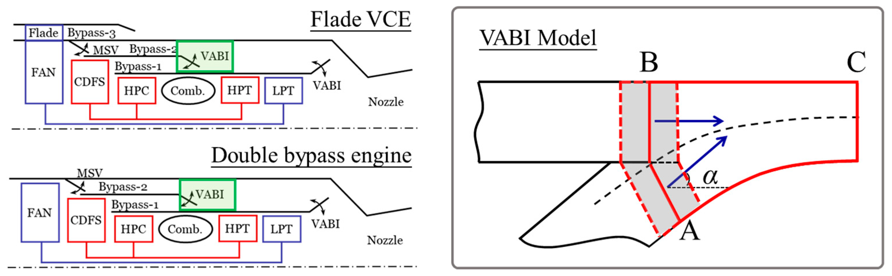
:1. Introduction
2. The Basic Control Volume Injection Flow Model
2.1. Basic Control Volume Model
2.2. Validation with Numerical Results
2.3. The Effect of the Streamline Curvature
3. An Improved Injection Flow Model
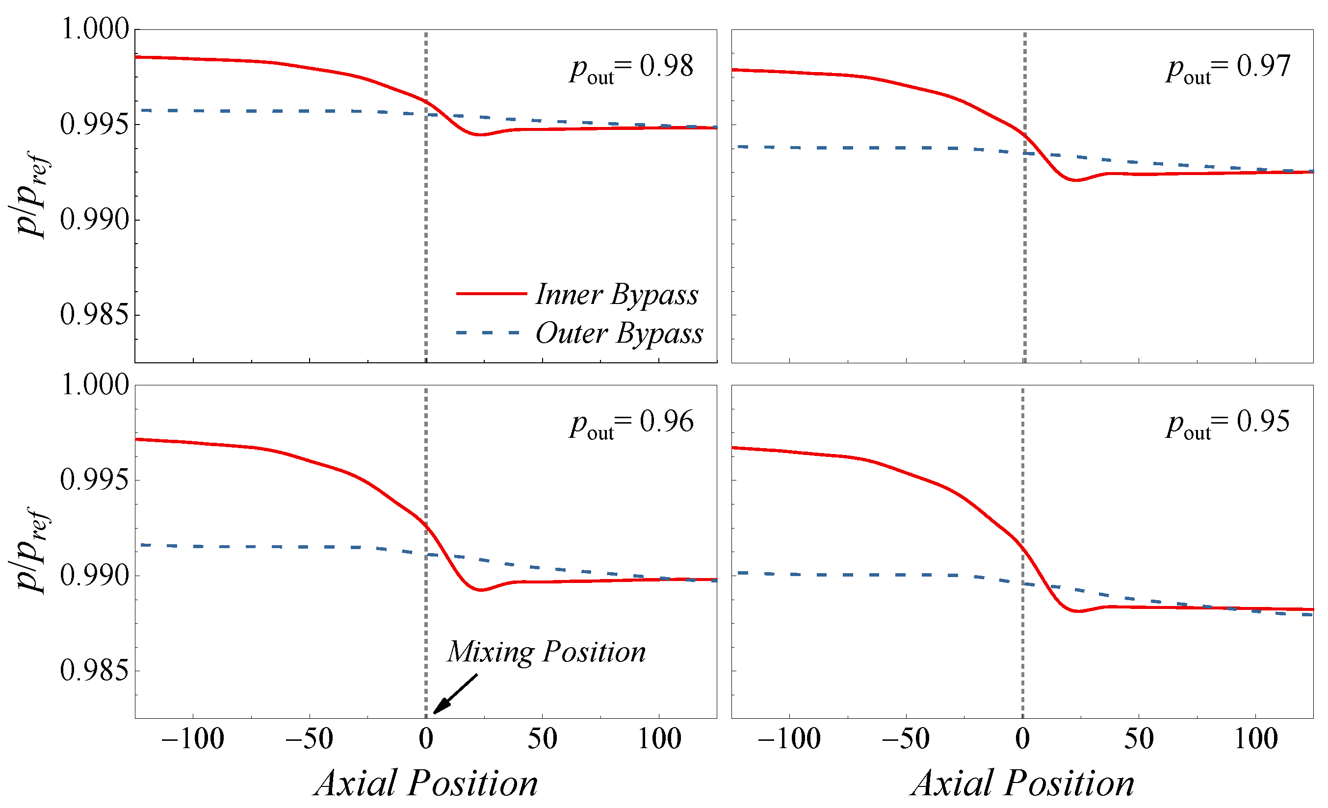
3.1. Consideration of the Mixing Flow Static Pressure Correction
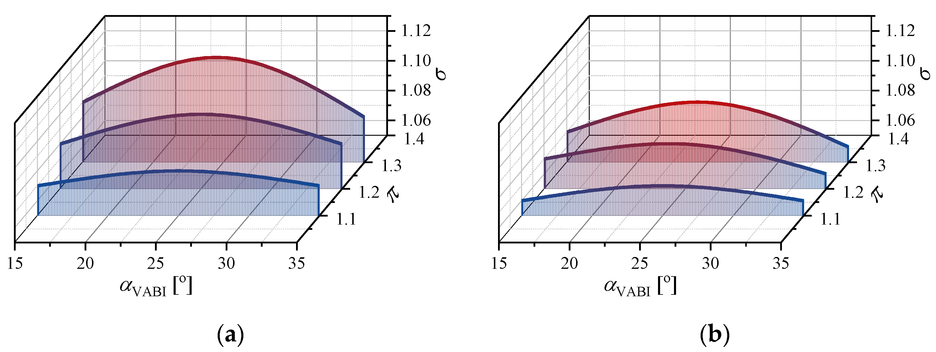
3.2. Calibration of the Improved Injection Flow Model
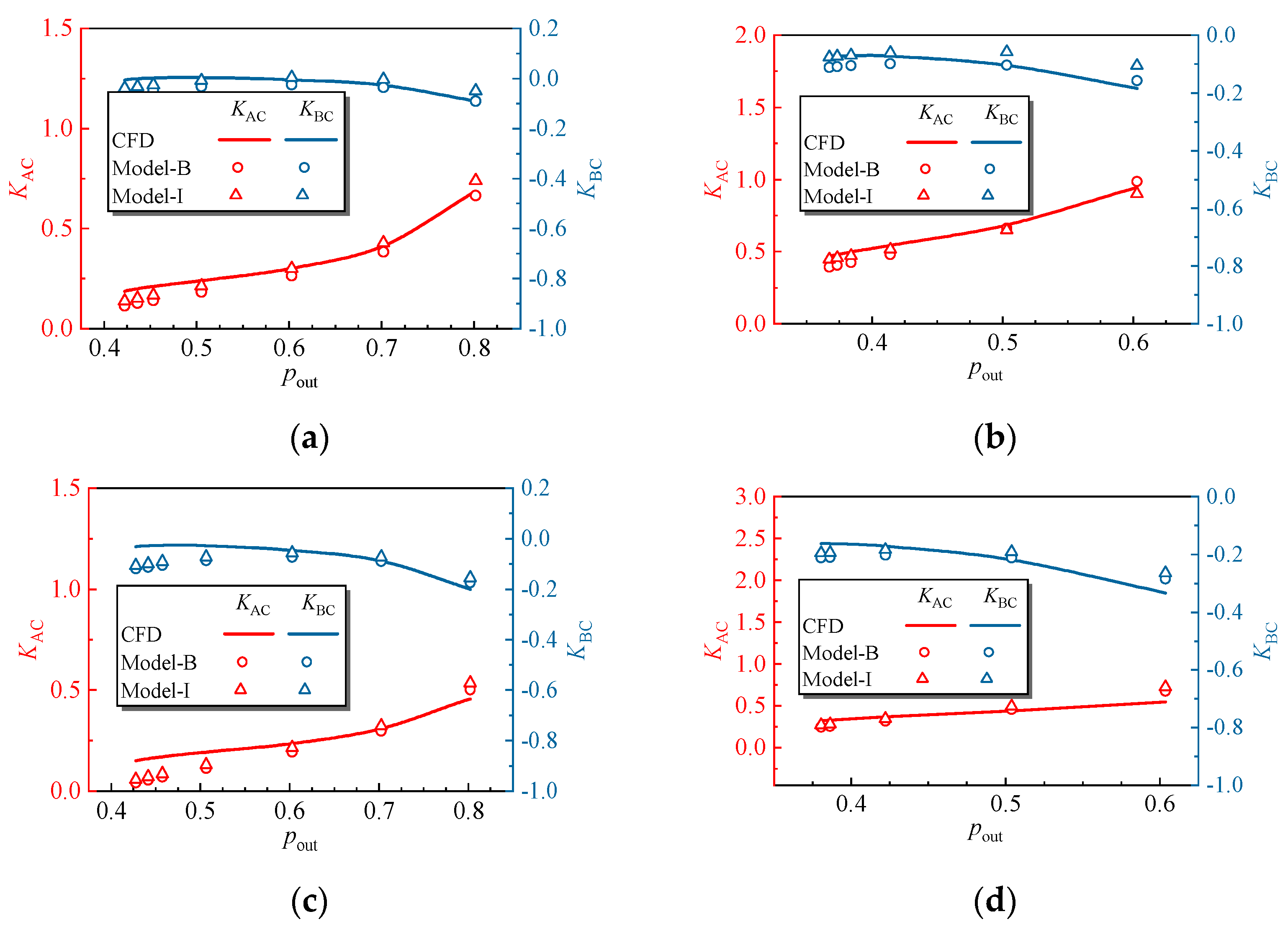
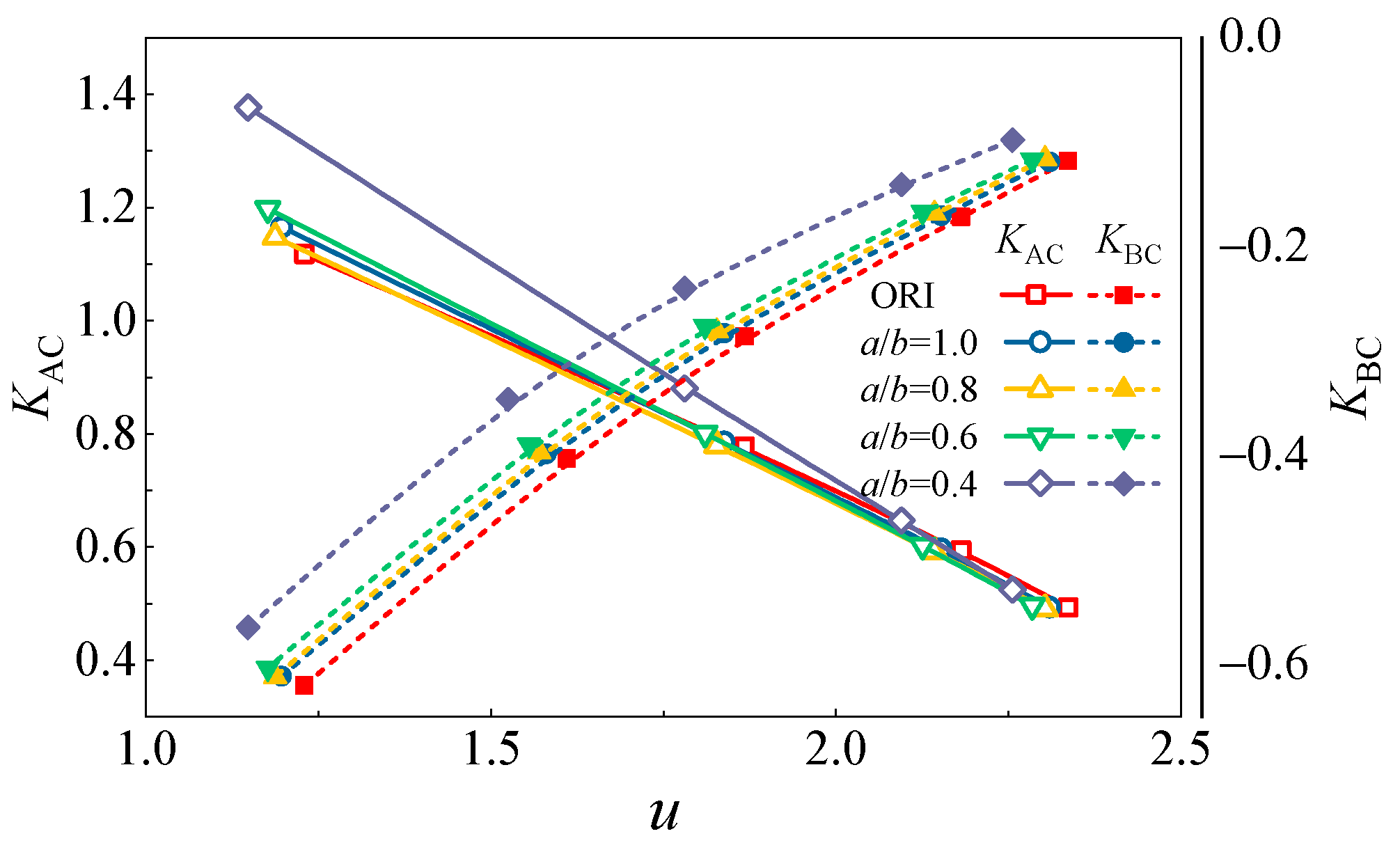
3.3. Validation of the Improved Injection Flow Model
4. Experimental Validation of the Improved Control Volume Model
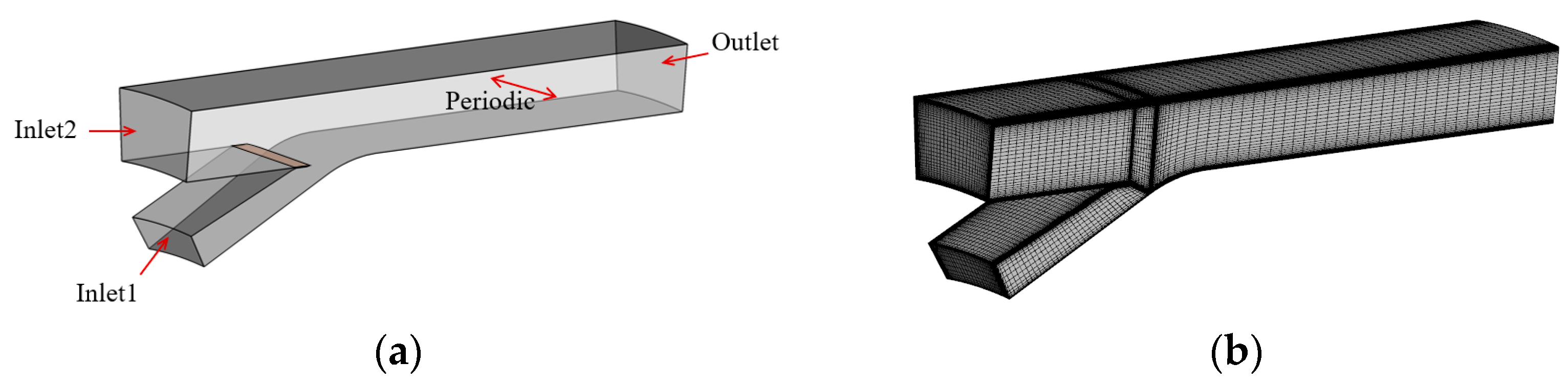
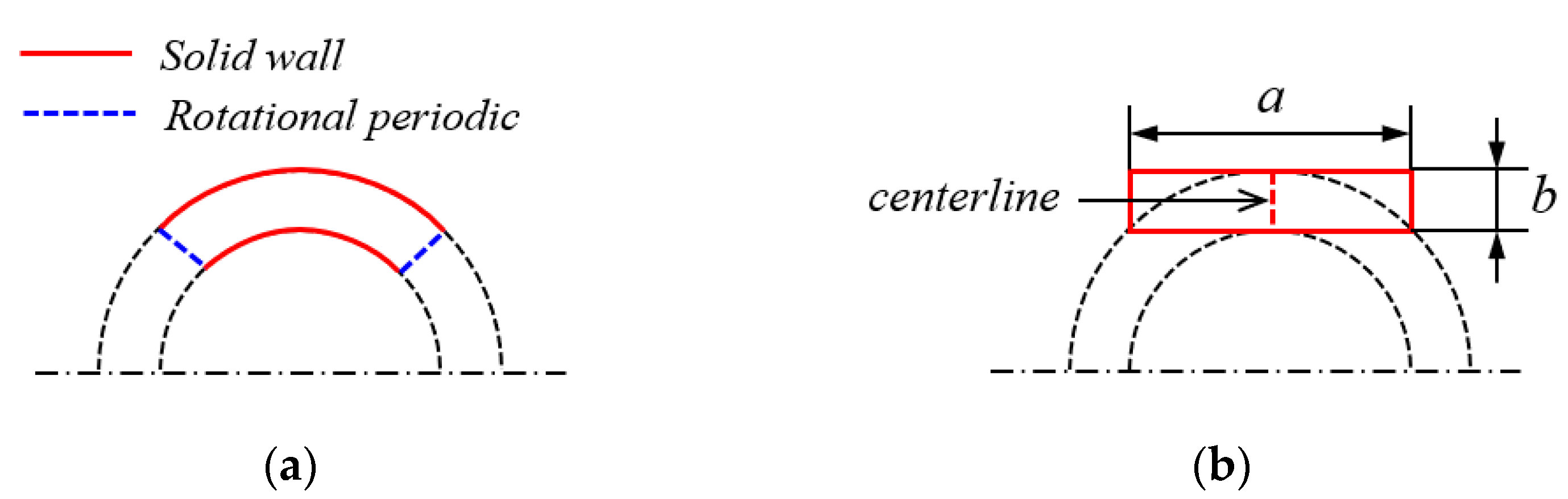
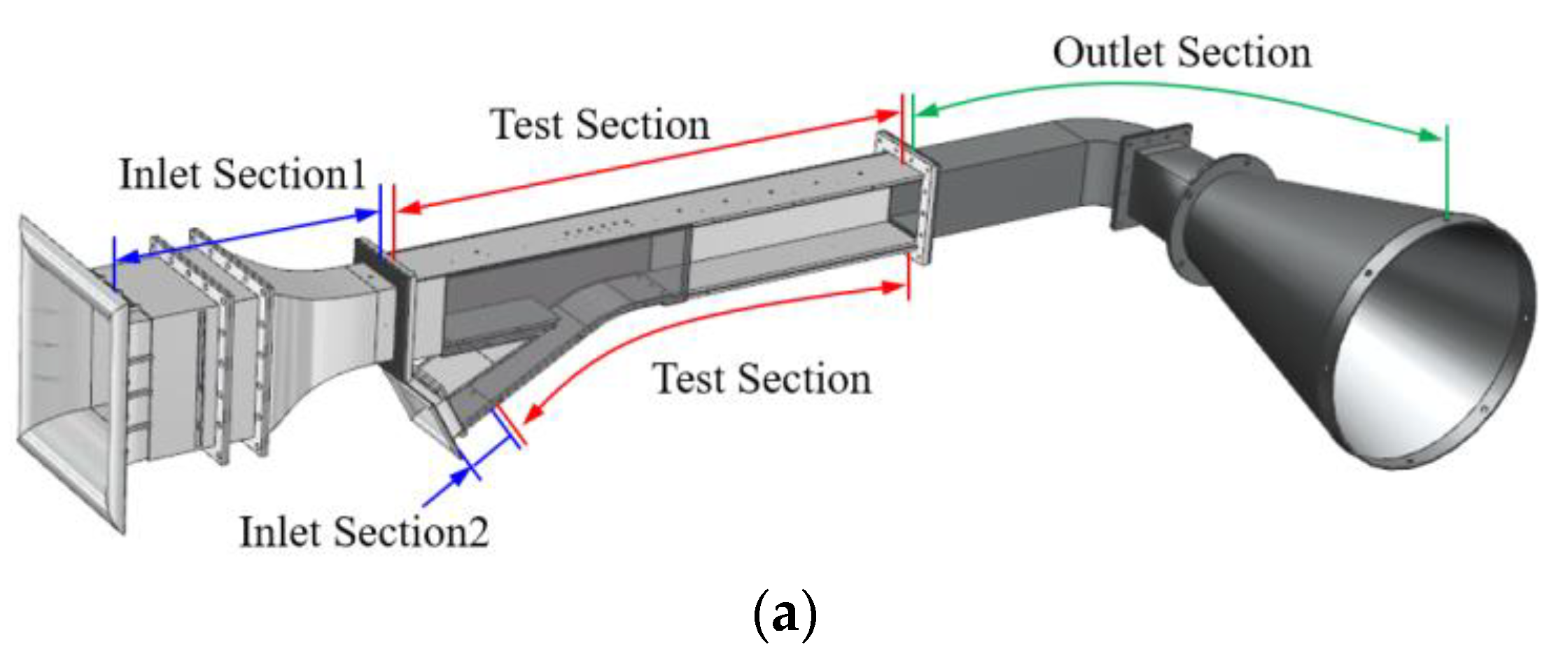
4.1. Design of a Simplified Injection Flow Test Model
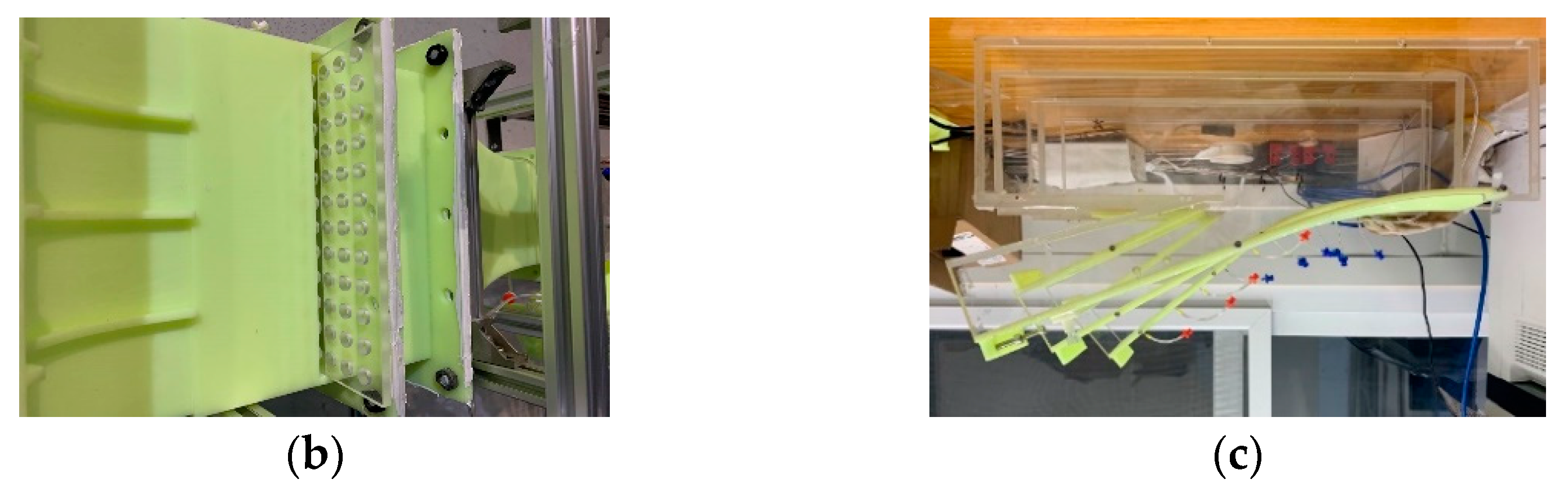
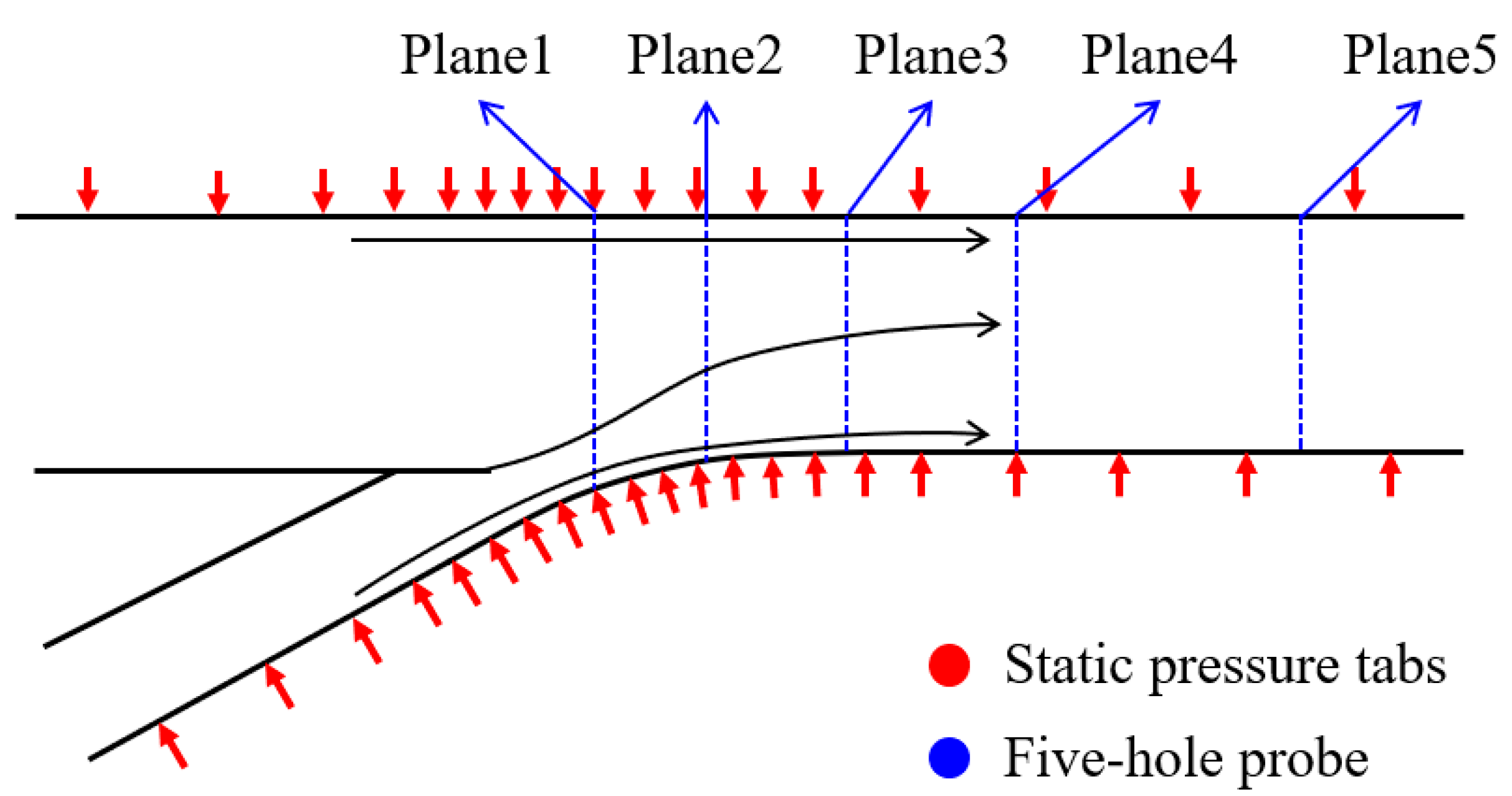
4.2. Experimental Setup
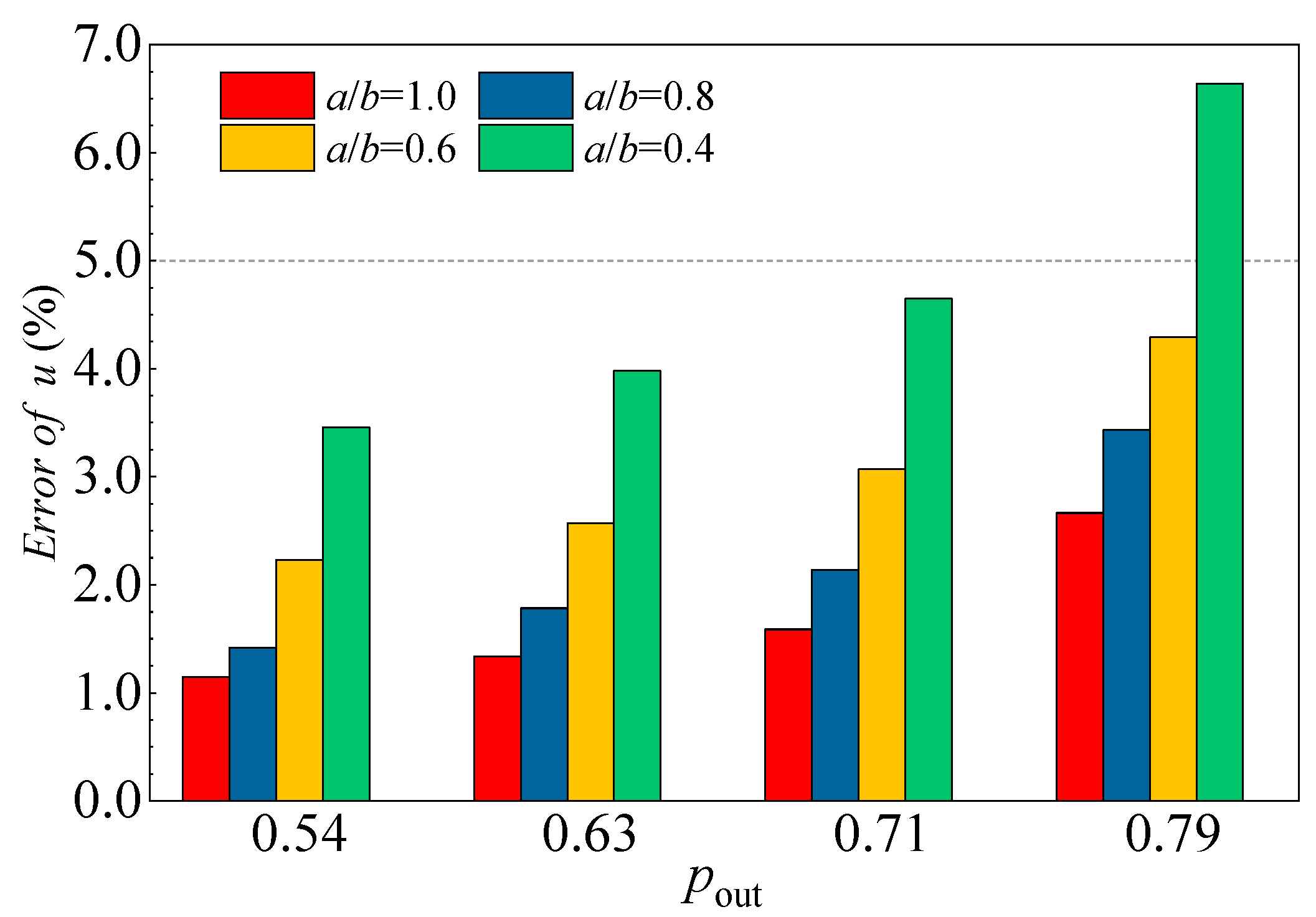
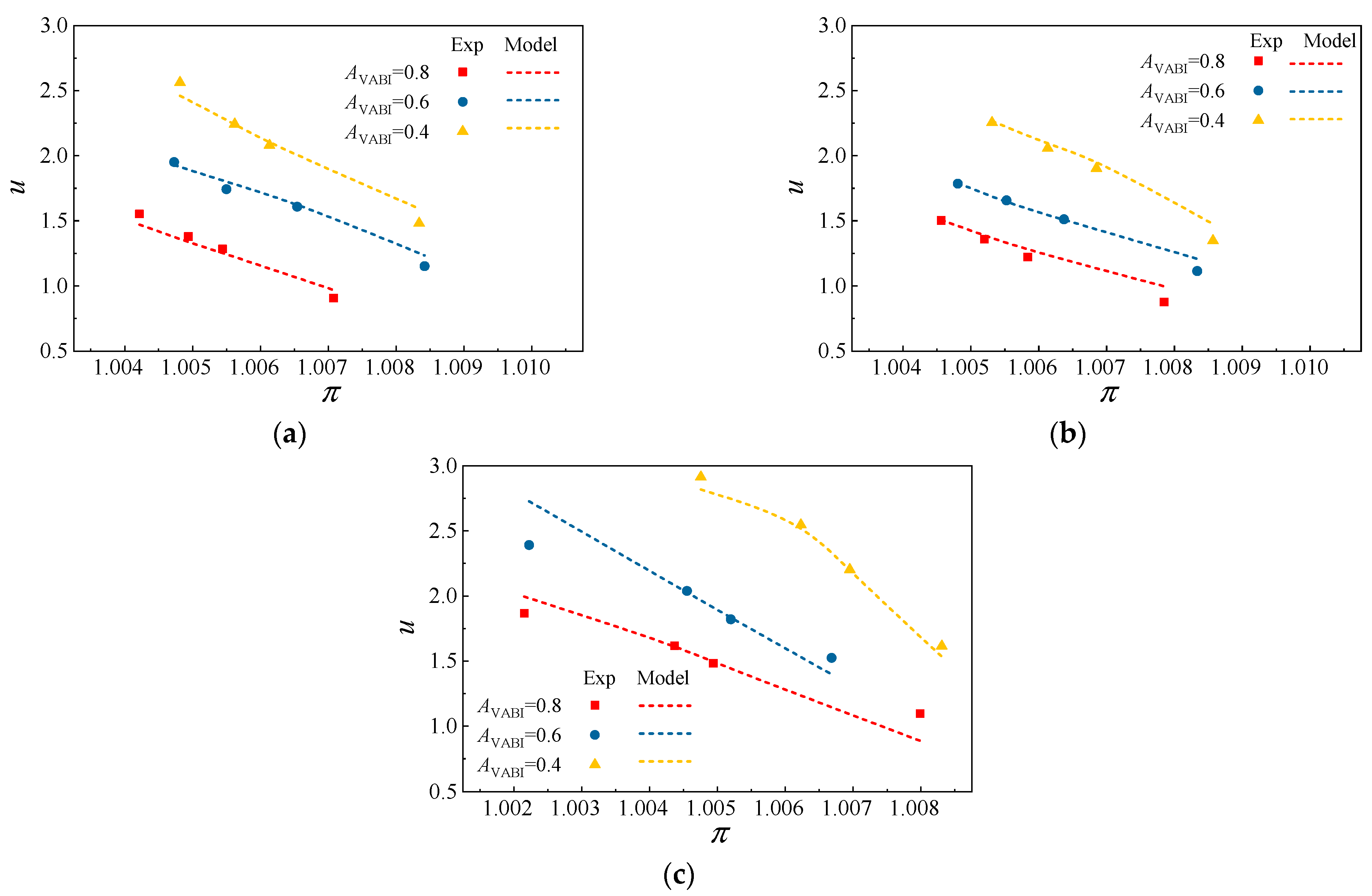
4.3. Model Validation
5. Conclusions
Author Contributions
Funding
Institutional Review Board Statement
Informed Consent Statement
Data Availability Statement
Acknowledgments
Conflicts of Interest
References
- General Electric. GE Successfully Concludes Phase 1 Testing on Second XA100 Adaptive Cycle Engine. 2021. Available online: https://www.ge.com/news/press-releases/ge-successfully-concludes-phase-1-testing-on-second-xa100-adaptive-cycle-engine (accessed on 15 December 2021).
- Zheng, J.C.; Chen, M.; Tang, H.L. Matching mechanism analysis on an adaptive cycle engine. Chin. J. Aeronaut. 2017, 30, 706–718. [Google Scholar] [CrossRef]
- Vyvey, P.; Bosschaerts, W.; Villace, V.F.; Paniagua, G. Study of an airbreathing variable cycle engine. In Proceedings of the 47th AIAA/ASME/SAE/ASEE Joint Propulsion Conference & Exhibit, San Diego, CA, USA, 31 July–3 August 2011. [Google Scholar] [CrossRef]
- Allan, R.D. General Electric company variable cycle engine technology demonstrator programs. In Proceedings of the 15th Joint Propulsion Conference, Las Vegas, NV, USA, 18–20 June 1979. [Google Scholar] [CrossRef]
- Johnson, J.E. Variable cycle engine developments at General Electric-1955-1995. In Developments in High-Speed Vehicle Propulsion System; Murphy, S., Curran, E.T., Eds.; AIAA: Reston, VA, USA, 1996; pp. 105–158. [Google Scholar] [CrossRef]
- Conrad, D.W.; Guy, K.F. Individual Bypass Injector Valves for a Double Bypass Variable Cycle Turbofan Engine. U.S. Patent US4175384, 27 November 1979. [Google Scholar]
- Simmons, R.J. Design and Control of a Variable Geometry Turbofan with and Independently Modulated Third Stream. Ph.D. Thesis, The Ohio State University, Columbus, OH, USA, 2009. [Google Scholar]
- Bachelder, K.A.; Welty, D.J. Methods and Apparatus for Supporting Variable Bypass Valve Systems. U.S. Patent US6742324B2, 1 June 2004. [Google Scholar]
- Keenan, J.H.; Neumann, E.P.; Lustwerk, F. An investigation of ejector design by analysis and experiment. J. Appl. Mech. 1950, 17, 299–309. [Google Scholar] [CrossRef]
- Goff, J.A.; Coogan, C.H. Some two-dimensional aspects of the ejector problem. J. Appl. Mech. 1942, 9, A151–A154. [Google Scholar] [CrossRef]
- Hedges, K.R.; Hill, P.G. Compressible flow ejectors: Part I—Development of a finite-difference flow model. J. Fluids Eng. 1974, 96, 272–281. [Google Scholar] [CrossRef]
- Besagni, G.; Mereu, R.; Inzoli, F. Ejector refrigeration: A comprehensive review. Renew. Sust. Energ. Rev. 2016, 53, 373–407. [Google Scholar] [CrossRef] [Green Version]
- Al-Nimr, M.A.; Tashtoush, B.; Hasan, A. A novel hybrid solar ejector cooling system with thermoelectric generators. Energy 2020, 198, 117318. [Google Scholar] [CrossRef]
- Yang, Y.; Karvounis, N.; Walther, J.H.; Ding, H.B.; Wen, C. Effect of area ratio of the primary nozzle on steam ejector performance considering nonequilibrium condensations. Energy 2021, 237, 121483. [Google Scholar] [CrossRef]
- Xu, Z.W.; Li, M.; Tang, H.L.; Chen, M. A multi-fidelity simulation method research on front variable area bypass injector of an adaptive cycle engine. Chin. J. Aeronaut. 2022, 35, 202–219. [Google Scholar] [CrossRef]
- Song, F.; Zhou, L.; Wang, Z.X.; Lin, Z.F.; Shi, J.W. Integration of high-fidelity model of forward variable area bypass injector into zero-dimensional variable cycle engine model. Chin. J. Aeronaut. 2021, 34, 1–15. [Google Scholar] [CrossRef]
- Huang, G.P.; Li, C.; Xia, C.; Li, Q. Investigations of entrainment characteristics and shear-layer vortices evolution in an axisymmetric rear variable area bypass injector. Chin. J. Aeronaut. 2022, 35, 230–244. [Google Scholar] [CrossRef]
- Zhang, B.L.; Liu, H.; Zhou, J.H.; Liu, H. Experimental research on the performance of the forward variable area bypass injector for variable cycle engines. Int. J. Turbo Jet Eng. 2020. [Google Scholar] [CrossRef]
- Benson, R.S.; Woollatt, D.; Woods, W.A. Unsteady flow in simple branch systems. Proc. Inst. Mech. Eng. 1963, 178, 24–49. [Google Scholar] [CrossRef]
- Bassett, M.D.; Winterbone, D.E.; Pearson, R.J. Calculation of steady flow pressure loss coefficients for pipe junctions. Proc. Inst. Mech. Eng. Part C 2001, 215, 861–881. [Google Scholar] [CrossRef]
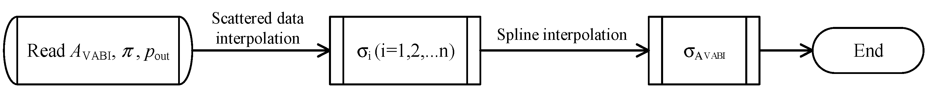
- Amidror, I. Scattered data interpolation methods for electronic imaging systems: A survey. J. Electron. Imaging 2002, 11, 157–176. [Google Scholar] [CrossRef]
- Miller, D.S. Internal Flow Systems, 2nd ed.; BHRA: Bedford, UK, 1990; pp. 87–91. [Google Scholar]
- Abou-Haidar, N.I.; Dixon, S.L. Pressure losses in combining subsonic flows through branched ducts. J. Turbomach. 1992, 114, 264–270. [Google Scholar] [CrossRef]
- Wang, R.Y.; Liu, B.J.; Yu, X.J.; An, G.F. The exploration of bypass matching limitation and mechanisms in a double bypass engine compression system. Aerosp. Sci. Technol. 2021, 119, 107225. [Google Scholar] [CrossRef]
- Liu, B.J.; Qiu, Y.; An, G.F.; Yu, X.J. Utilization of zonal method for five-hole probe measurements of complex axial compressor flows. J. Fluids Eng. 2020, 142, 061504. [Google Scholar] [CrossRef]
- Liu, B.J.; An, G.F.; Yu, X.J.; Zhang, Z.B. Experimental investigation of the effect of rotor tip gaps on 3D separating flows inside the stator of a highly loaded compressor stage. Exp. Therm. Fluid Sci. 2016, 75, 96–107. [Google Scholar] [CrossRef] [Green Version]


| Category | Parameter | Definition |
|---|---|---|
| Geometric parameter | Injection angle | α |
| VABI opening area | AVABI = AA/AB | |
| Aerodynamic parameter | Bypass backpressure | pout = pC/pA* 1 |
| Bypass total pressure ratio | π = pA*/pB* | |
| Injection ratio | u = mB/mA |
| Variation Range | |
|---|---|
| AVABI | (0.2, 0.8) step = 0.2 |
| π | (1.1, 1.5) step = 0.1 |
| pout | (0.1, 1.5) step = 0.1 |
| Case | A01 | A02 | A03 | A04 |
|---|---|---|---|---|
| Scale factor | 2.0 | 1.5 | 1.0 | 0.8 |
| Reynolds number | 350,000 | 262,500 | 175,000 | 140,000 |
| Case | C01 | C02 | C03 |
|---|---|---|---|
| αVABI (°) | 35 | 25 | 15 |
| AVABI | 0.4~0.8 | 0.4~0.8 | 0.4~0.8 |
Publisher’s Note: MDPI stays neutral with regard to jurisdictional claims in published maps and institutional affiliations. |
© 2022 by the authors. Licensee MDPI, Basel, Switzerland. This article is an open access article distributed under the terms and conditions of the Creative Commons Attribution (CC BY) license (https://creativecommons.org/licenses/by/4.0/).
Share and Cite
Wang, R.; Yu, X.; Zhao, K.; Liu, B.; An, G. Development and Validation of a Novel Control-Volume Model for the Injection Flow in a Variable Cycle Engine. Aerospace 2022, 9, 431. https://doi.org/10.3390/aerospace9080431
Wang R, Yu X, Zhao K, Liu B, An G. Development and Validation of a Novel Control-Volume Model for the Injection Flow in a Variable Cycle Engine. Aerospace. 2022; 9(8):431. https://doi.org/10.3390/aerospace9080431
Chicago/Turabian StyleWang, Ruoyu, Xianjun Yu, Ke Zhao, Baojie Liu, and Guangfeng An. 2022. "Development and Validation of a Novel Control-Volume Model for the Injection Flow in a Variable Cycle Engine" Aerospace 9, no. 8: 431. https://doi.org/10.3390/aerospace9080431