Article

Aerodynamic Analysis of a Supersonic Transport Aircraft at Low and High Speed Flow Conditions

Engineering Department, Università della Campania “L.Vanvitelli”, Via Roma 29, I-81031 Aversa, CE, Italy
*
Author to whom correspondence should be addressed.
Aerospace 2022, 9(8), 411; https://doi.org/10.3390/aerospace9080411
Submission received: 18 June 2022 / Revised: 23 July 2022 / Accepted: 26 July 2022 / Published: 29 July 2022
(This article belongs to the Special Issue Supersonic and Hypersonic Transportation Systems)

Abstract

:
The recent improvement of technology readiness level in aeronautics and the renewed demand for faster transportation are driving the rebirth of supersonic flight for commercial aviation. However, the design of a future supersonic aircraft is still very challenging due to the complexity of several problems, such as static stability performance during the acceleration phase from subsonic speeds to supersonic speeds. Additionally, the interest of scientific community in open source numerical platform as a valid tool for a reliable and affordable aerodynamic design is considerably growing. In this framework, the present work addresses the aerodynamic performance of a Concorde-like aeroshape developed within the preliminary design of a high-speed civil transportation aircraft. Several flight conditions, ranging from subsonic to supersonic speeds, were investigated in detail by using Computational Fluid Dynamics. The aerodynamic force and moment coefficients are computed with fully three-dimensional and steady state Reynolds Average Navier-Stokes simulations, carried out in turbulent flow conditions. The effect of the Mach number variation on the shift of the aircraft aerodynamic center is detailed, by focusing on the aircraft pitching static stability. Flowfield numerical simulations are performed with both commercial (Ansys-Fluent) tool and open-source (SU2) code, which is also used extensively in multidisciplinary design procedures, for further comparisons. Particular attention is focused on the shift of the aeroshape aerodynamic center to verify that the provided wing design allows the aircraft static margin to be within 5% of the reference length, both at low-speed and high-speed flight conditions. The computed positions of the aerodynamic center are in agreement with the aeroshape surface pressure distributions and confirmed the literature results available for the Concorde aircraft. Therefore, in the view of future simulation campaigns for supersonic transportation aircraft, the present work aims to bridge the gap between previous aerodynamic design experiences, for instance matured on Concorde, and those carried out with modern CFD tools on full-scale aircraft, and on time-scales compatible with conceptual design practice. Finally, as the difference between the computed aerodynamic coefficients reflected mainly on drag computation performed with SU2, a special focus on numerical diffusion effect of the solver is also given and compared with a commercial certified CFD tool. This adds a unique further contribution to the SU2 community for aeronautics application.

1. Introduction

Recent studies performed by aerospace industries demonstrated that faster aircrafts improves both business and international relationships while reducing time connections [1]. Regular market of business-class fare gives special attention to time spent during flight. Therefore, companies like Boom and Boeing are focusing on this peculiar aspect by relying on a wider demand of faster flights [2,3,4,5,6,7]. Several U.S. companies are currently proposing new Supersonic Aircraft (SA) prototypes, which represent the future for business class routes [1,8]. Supersonic aircraft concepts, namely AS2, S-512, and Overture, are the ongoing development carried on by Aerion, Spike Aerospace, and Boom aircraft companies, respectively [9,10,11]. While the AS2 and the S-512 concepts belong to the business jet segment, Overture is a larger Mach 2.2 High Speed Civil Transportation (HSCT) aircraft, having transport capability of about fifty passengers and a range of nearly 5000 nm [1,11].
In this scenario, aircraft designers are facing two challenging problems i.e., the environmental effects due to supersonic aviation and noise emission due to sonic boom, which actually represents the strongest barriers to supersonic flight [8,12]. The environmental focus is related to the lowering of greenhouse gas and pollutant emissions and demands to implement strategies to comply with the sustainability standard of International Civil Aviation Organization (ICAO). The objective is set to a 50% reduction of aviation emissions related to C O 2 and N O x in the next future [13]. Additionally, a significant attention of designers is also focused on sonic boom mitigation. Actually, since Concorde last flight, sonic-boom is still the main design concern for commercial SA due to prohibition of supersonic overland flight [8,13,14,15,16]. Aside from the environmental issues related to sonic boom mitigation and reduction of fuel emissions, physics of supersonic flows is completely different from the one featuring the sub-transonic regime [17,18]. Many design criteria of SA are different from those adopted for low-speed regime. Specifically, longitudinal stability requirement of SA relates to peculiar aerodynamic phenomena characterising the supersonic regimes.
As matter of fact, aerodynamic characteristics radically change when aircraft accelerate from subsonic to supersonic speeds [19].
Among the most relevant changes, it is worth noting that the lift-to-drag ratio (L/D) strongly decreases and the aircraft Centre of Pressure (CoP) shifts backward, by affecting vehicle performance, static stability, and trimmability. The rearward movement of CoP determines a marked nose pitch-down tendency, known as Mach tuck phenomenon. Moreover, a marked rearward shift of CoP at M > 1 (i.e., increased distance between the CoP and the centre of gravity (CoG) ) determines a lower manoeuvrability and a large elevon deflection to trim the aircraft which, in turn, leads to an unacceptable large trim drag. Recall that stability considerations are, however, performed with reference to the Aerodynamic Center (AC) of the aircraft, also known as the vehicle neutral point. Differently to CoP, in fact, the pitching moment coefficient evaluated with respect to the AC does not depend on the AoA. Previously mentioned design concerns are even more challenging considering that for a SA the longitudinal stability requirement must be prescribed over a wide range of Mach numbers.
Aircraft longitudinal stability is investigated in literature by formulating mathematical problems which resume by MDO (Multidisciplinary Design Optimization) procedures [20]. Specifically, low-speed stability for SA is related to the peculiar slender-shaped wing-planform, as discussed in the papers of Seraj et al. and Gursul et al. [21,22]. Seraj et al. [21] performed an optimization study by minimizing the drag at supersonic cruise and considering the static margin as a stability constraint at low-speed. Authors found that pitch stability at subsonic speeds was enforced by increasing the leading edge thickness at the expense of a larger wave drag. Gursul et al. [22,23] studied and related the stability behaviour of delta shaped wings to flow separation which was dependent on the leading edge radius.
Furthermore, the aircraft behaviour consequent to vortex breakdown was analysed, and it was found that breakdown favoured the longitudinal instability. Longitudinal stability condition for SA was also studied at high speed by Mangano et al. [20], who considered a multipoint design optimization over a two-dimensional supersonic profile and over an ideal supersonic concept the Aerion AS2 in several flow regimes. The high-speed stability constraint was formulated in term of trim condition by constraining the pitching moment coefficient. Fukurawa et al. [16] studied a civil SA concept with sonic boom mitigation at supersonic speed. The stability condition in supersonic regime was used as objective function. Therefore, the absolute value of the static margin and the CoG was minimized. Because of the significant variation of pitching moment and drag coefficients a supersonic aircraft has to withstand during flight, its aeroshape must be accurately designed.
With this in mind, aircraft architectures made by appropriately combining slender low aspect ratio Delta wings (DW) and the Sears-Haack body fuselage represent the right design option. In fact, Sears-Haack bodies and DW are able to alleviate the wave drag at supersonic speeds. In addition, DW also at low-speed conditions provide interesting aerodynamic characteristics, namely the vortex lift phenomenon. At high Angle of Attack (AoA), DW promotes the creation of leading edge vortices which originate from the leading-edge separation, and consequent roll up of the oncoming airstream [24,25]. This vortex system increases the aerodynamic lift, according to the well known vortex lift phenomenon. Additionally, DW have the further advantage to limit the excursion of the CoP towards aircraft tail. It is shown in Ref. [26] that the Concorde ogee wing was designed to constraint the CoP displacement within a fixed range of the chord length at the wing root.
Within this framework, the present research effort addresses the aerodynamic analysis of a SA featuring a Concorde-like aeroshape by means of steady state, fully turbulent, and three-dimensional Reynolds Average Navier-Stokes (RANS) simulations, carried out in subsonic, transonic, and supersonic flow conditions. The aerodynamic force and moment coefficients are computed for different angles of attack and for longitudinal flight conditions only. The shift of the aeroshape AC is assessed in a wide rage of Mach number, and results are compared with literature data [26].
Flowfield numerical simulations are performed with both commercial Ansys-Fluent and open-source SU2 tools for further comparisons. The shift of the aircraft AC is related to the different pressure distributions predicted by CFD simulations both at low speed and high speed flight conditions. The computed positions of the AC are in agreement with the aeroshape surface pressure distributions and confirmed the literature results, available for the Concorde aircraft [26].

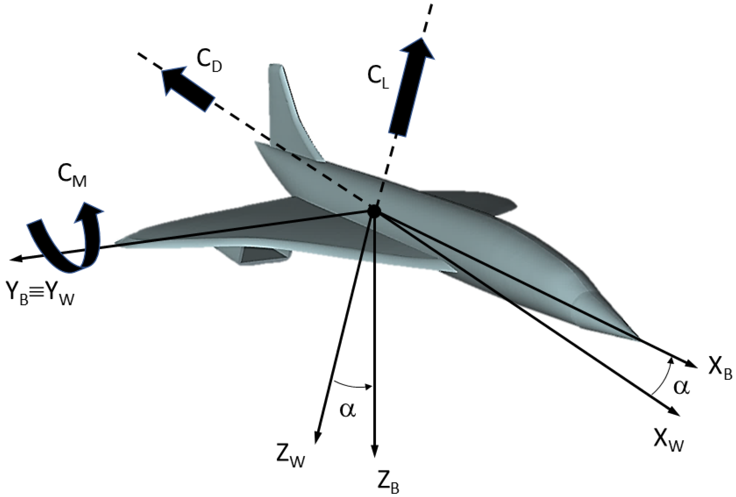
2. Aircraft Static Stability

The static stability and the trimmability of an aircraft is commonly formalised by evaluating the static margin of the vehicle defined as the distance between the CoG and the AC of the aircraft:
S M = X ¯ C o G X ¯ A C
where X ¯ C o G and X ¯ A C are the longitudinal dimensionless position (i.e., X ¯ i = X i / L r e f ) of the CoG and AC, respectively. The aircraft static stability is indeed resumed by the following relationship:
C M C L = X ¯ C o G X ¯ A C < 0
when X ¯ C o G < X ¯ A C the aircraft is considered statically stable (i.e., C M α < 0 ). Otherwise, for X ¯ C o G > X ¯ A C the aircraft is statically unstable (i.e., C M α > 0 ).
Stability of SA becomes problematic during the transition between the subsonic and the supersonic regime. In fact, while flow physics imposes to the AS to move backward during the acceleration phase, there are no natural reasons that determine changes in CoG position. So that, when the SA accelerates to supersonic speed the X C o G remains unchanged while the AC moves [27]. As a result, the shift of the AC is one among the major concern for a reliable SA design. If the aircraft is designed to have CoG by allowing a proper SM at subsonic speeds, the SM eventually becomes unacceptably large at supersonic speeds. In addition, if aircraft design provides a CoG located to achieve a proper SM at supersonic speeds, the subsonic SM most likely would be negative (i.e., AC ahead of the CoG), hence making the aircraft unstable in subsonic flight. Thus, two different solutions to overcome the stability and manoeuvrability issues can be adopted for SA.
On one hand, the CoP can be maintained at the CoG location by trimming the aircraft using a suitable elevon deflection. However, this solution requires an additional elevon oversizing with a consequent increase of trim drag.
On the other hand, the X C o G could be moved backward (i.e., CoG control) in order to limit the increase of the aircraft SM. For instance, this was the design solution adopted for the Concorde aircraft. In that case, the shift of the CoG was performed with a fuel pumping system which transferred the fuel from fore to the aft tank of the aircraft, namely rear trim tank [26]. When crossing the sound barrier, Concorde uses afterburners. Therefore, during the acceleration to Mach 2, the fuel is pushed towards the tail producing an additional retraction of the CoG [26].
Conversely, during the deceleration, fuel is pumped forward to compensate the forward shift of the AC, thus establish the static equilibrium at subsonic condition [26]. In addition, in order to further limit the aircraft SM, the wing planform of Concorde was opportunely chosen, by adopting an ogee delta wing. In fact, the Concorde ogee-planform wing, helped to constraint the shift of AC in cruise conditions within about 62% of the length of the wing root chord.
Finally, it is worth noting that another advantage in moving the CoG of the aircraft consisted in the possibility of using the internal elevons of the Concorde to trim the aircraft to a certain attitude. In fact, without shifting the CoG high elevon deflections were required, which were impossible due to the Concorde operating range in cruising conditions (i.e., M = 2.02 ) [26].

3. Aerodynamic Analysis

Aircraft aerodynamics and static stability in longitudinal flight conditions are addressed in the current sections for the whole flight scenario of the vehicle. The shift of the AC (i.e., the aircraft neutral point) expected during the acceleration phase from subsonic to supersonic speeds is also discussed in detail. Flow modelling and simulations procedures are detailed hereinafter.

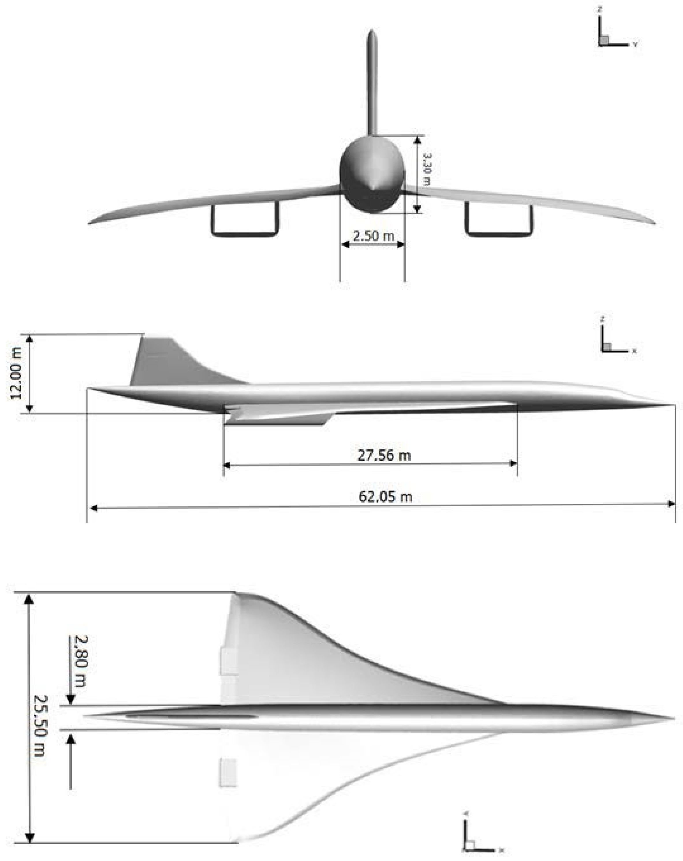
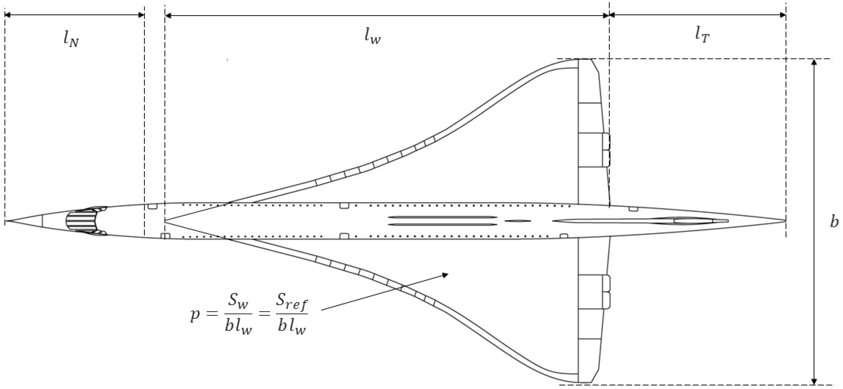
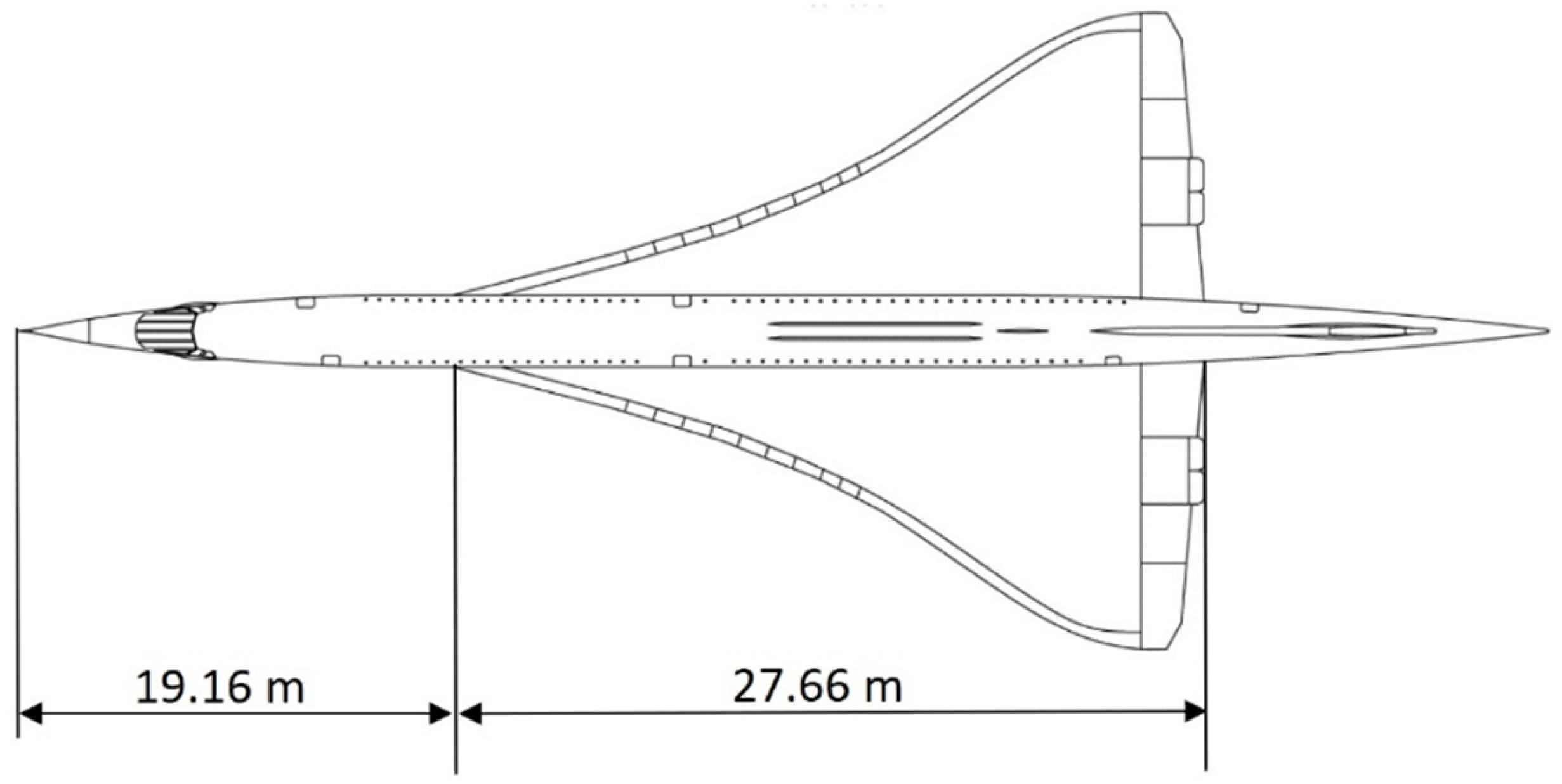
3.1. Aircraft Configuration

Generally speaking, a SA aeroshape essentially blends two different airplanes concepts. SA is optimized for the supersonic cruise, but at the same time optimal shapes are also designed to efficiently cover some segments of their trajectory at subsonic speeds (e.g., takeoff and landing).
With this in mind, the aircraft configuration under investigation is shown in Figure 1. As one can see, it features a Concorde-like aeroshape with a low mounted thin delta wing, seamlessly integrated within a Sears-Haack body fuselage, and a tailless configuration, as used for the Concorde and the Tupolev Tu-144 airplanes. The configuration also features a quite constant cross section fuselage with considerable nose overhang relative to an ogee wing. This aeroshape was obtained starting from high-level requirements of 80–100 passengers, a supersonic cruise up to Mach 1.5–2.0 (1590–2120 km/h; 859–1145 kn) at an altitude of 60,000 ft (18.3 km), and a range of 4000–4500 nmi (7400–8334 km). To cope with these requirements, an aircraft architecture with a tailless and a narrow fuselage integrated with a low aspect ratio delta wing with cropped wingtips was chosen, like those adopted for the Concorde and Boom Overture aircraft. Therefore, the planform view features a long, slim fuselage and a slender delta wing with its distinctive ogee leading edge, long root chord and short span. In particular, design requirements lead to a first instance aircraft 65 m long and with 27 m as wingspan. These dimensions were refined while design matured, as shown in Figure 1.
The slender high fineness ratio fuselage (i.e., needle-like shape) was obtained starting from a Sears-Haack body, which also satisfied the area rule, to limit drag at high-speed conditions. In fact, the fuselage design depends on the wave drag coefficient ( C D w ) which increases rapidly as the fuselage volume (V) increases:
C D w = 24 V L 3 S m a x S r e f = 9 π 2 2 R m a x L S m a x S r e f = 4.69 4 R m a x 2 l N 2 + R m a x 2 l T 2 S m a x S r e f
where R m a x is the body maximum radius, S m a x and L are its maximum cross-section area and length, respectively. S r e f is the aircraft aerodynamic reference surface, l N and l T are the lengths of nose and tail parts of the aircraft (see Figure 2) [19,28]. A double-bubble cross-sectional layout was considered to separate areas for cabin and cargo.
The wing and the tail were designed in order to provide the aircraft with a suitable aerodynamic performance throughout the flight envelope, especially at high-speed conditions. In fact, according to Ref. [19], their wave drag coefficient reads:
C D w = 512 π ν p s 2 K 0 β s S w e t , e a c h 2 S r e f
where s is the slenderness ratio of the part; for the wing:
s = b 2 l w
p is the planform parameter of the part; for the wing:
p = S r e f b l w
ν is the volume parameter of the part; for the wing:
ν = V S r e f 3 2
being V the volume of the part; in addition
β = M 2 1
K 0 is an empirical coefficient for wave drag due to volume and S w e t , e a c h is the wetted area of each part.
A NACA 64A series airfoil was chosen with a thickness ranging from 3% at root up to about 2% at tip; the wingspan was determined according to the Mach’s cone semi aperture angle at cruise speed (i.e., the wing leading edge remains behind the shock cone created by the leading-edge root); the ogival delta wing was compound-rounded into the shape of a smooth ogee equal to that of the Concorde wing. Therefore, the high sweptback leading-edge and low thickness/chord ratio improved wave drag. Furthermore, the high leading-edge sweep at the root (i.e., wing strakes) determines, at low speed, strong controlled counter-rotating vortices on the leeside at high angles of attack. Such vortices lower the local air pressure and cause high-lift (i.e., vortex-lift phenomenon), thus improving aircraft low speed performance, such as take-off and landing speeds. A detailed description of the vortex lift phenomenon that takes place over this ogee wing at very low speeds can be found in Ref. [24].
According to the Concorde design, the ogee wing planform helps in reducing the amount of control force required to pitch trim the aircraft. In fact, the movement of the aerodynamic center between low speed and supersonic cruise conditions is reduced (i.e., low static margin both at low speed and in supersonic cruise). This way, the trim of the aircraft in cruise for minimum drag was accomplished by means of fuel transfer to adjust the centre of gravity in supersonic flight and with a proper camber and twist of the wing.
Finally, the pitch down tendency of the sweptback wing is counterbalanced by four engines placed beneath the wing and on the rear part of it. This arrangement has also the advantage to determine a lighter wing since allows the engine weight to counteract the wing lift, thus reducing the wing root bending moment.

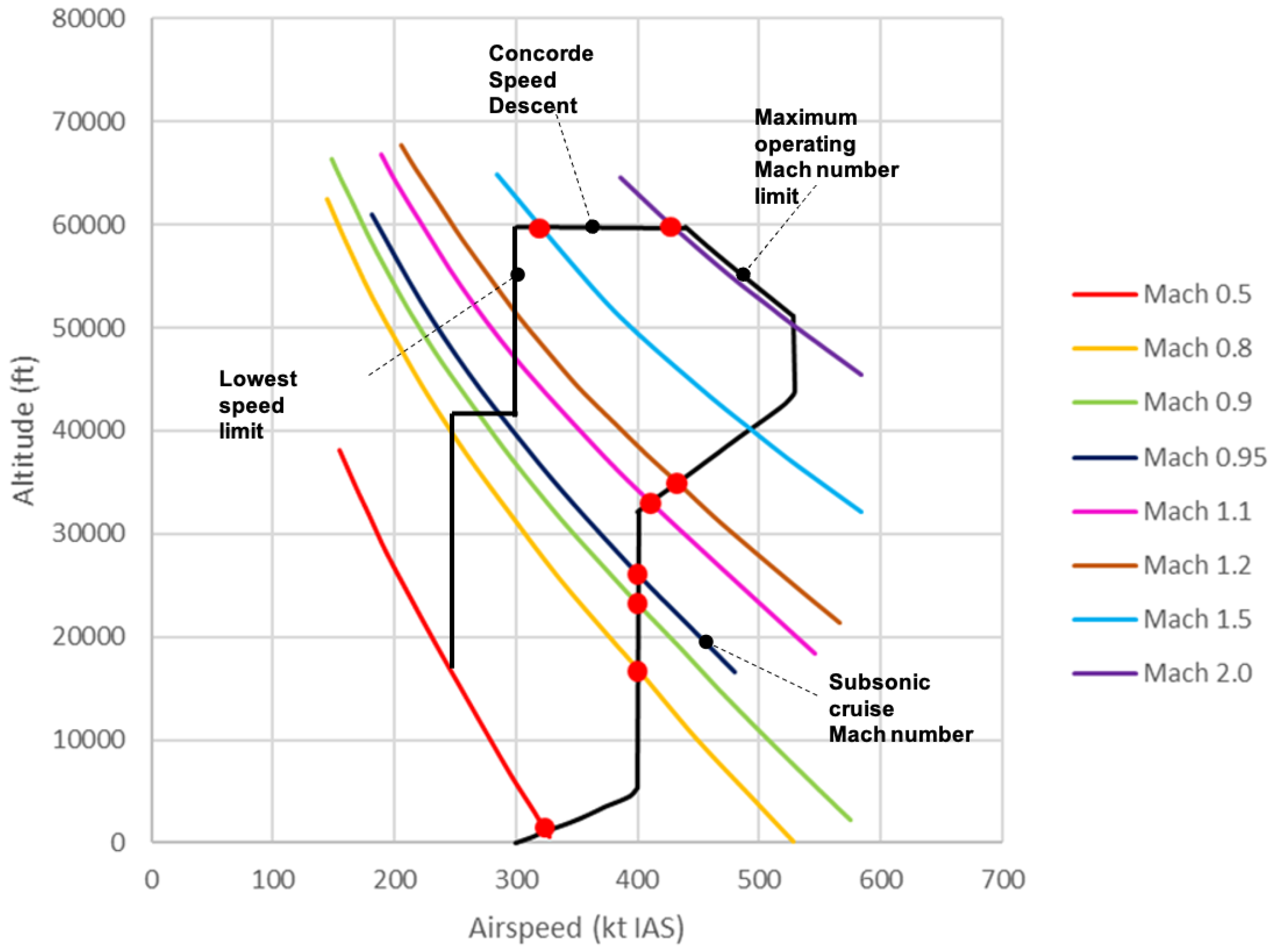
3.2. Flight Envelope

The Concorde flight envelope (FE), shown in Figure 3 and reported in Ref. [27], was assumed as reference for this aerodynamic study [26,29]. As shown, iso-Mach curves are also drawn to appreciate the Mach number variation expected during flight.
The Concorde FE is limited in terms of speed; the maximum operating speed limits ( V m o ) is set at about 530 knots IAS at 43,750 ft, where Mach number equals 2.04. Another limit set at 300 knots is represented by the lowest speed limit achievable.
In addition, it is worth noting that the aircraft is characterized by an extended FE subjected to significantly different design requirements (with a wide range of airspeed while altitudes extend up to about 18 km (60 kft), which adds further complications to the design of SA [26,29].

3.3. CFD Test Matrix

Aircraft aerodynamics and static stability in longitudinal flight conditions are addressed by means of CFD simulations which are performed at several Mach numbers from M = 0.24 to M = 2.0 , according to the FE in Figure 3.
Eleven control points along with the flight profile were considered to perform aircraft aerodynamic analysis.
The selected flight conditions refer to M = 0.24 , 0.5 , 0.8 , 0.9 , 0.95 , 1.02 , 1.1 , 1.2 , 1.5 , 1.8 , and 2.0 . For each Mach number, CFD simulations were carried out at different angles of attack, according to the CFD test matrix in Table 1. For the sake of simplicity, only low values of the AoA have been considered, namely α = 0 , 3 , 5 , and 10 d e g , since the focus is on the shift in the position of the aeroshape aerodynamic centre which, as is well known, does not depend on α .
Each simulated Mach number corresponds to a fixed height and cruise speed (i.e., R e , M ) of the FE. Therefore, aircraft aerodynamics and static stability in longitudinal flight conditions are addressed by means of twenty seven steady state, three-dimensional, and fully turbulent Navier-Stokes (NS) CFD simulations.

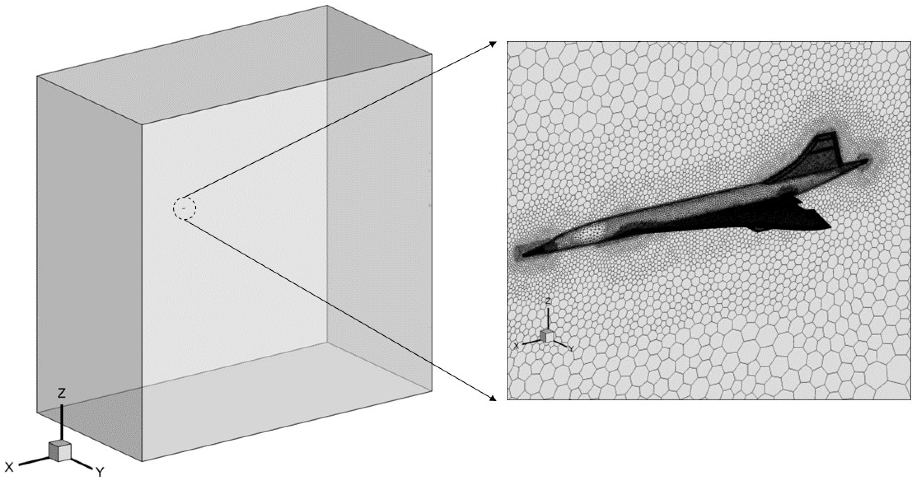
3.4. Grid Generation

Flowfield simulations were carried out on several quite different grids, according to the different free-stream Mach numbers summarized in the CFD test matrix (see Table 1). All grids are unstructured hybrid mesh with hexagonal or polyhedral cells in the flowfield domain, prisms in the boundary layer and triangular elements on the surface of the aircraft.
In particular, two computational domains were generated for the CFD simulations: one for subsonic simulations and the other one for supersonic computations. The fluid domain for the subsonic case is a prismatic brick with dimensions of length, width, and depth equal to fifty times the body-length of the aircraft. The subsonic computational domain is shown in Figure 4, where the mesh on the aircraft wall and symmetry plane is also provided.
On the other hand, for the supersonic case, the computational domain is different with respect to the subsonic one. In fact, due to the hyperbolic nature of the supersonic flow-field equations it features a paraboloid-like domain. To carry out simulations with Mach number ranging from 1.1 up to 2.0, the lowest Mach value was chosen for the paraboloid semi-aperture angle.
The supersonic computational domain is shown in Figure 5, where the mesh on the aircraft wall and symmetry plane is also provided.
To facilitate a correct transition in the growth of the size of adjacent tetrahedral cells, density boxes have been defined at the nose, at the leading edge of the wing, at the engine, and at the wing tip.
The boundary layer region has been discretized by exploiting prismatic inflation layers. The grid featured a minimum wall spacing equal to 10 6 m to allow for y + = O 1 and to describe the viscous sublayer.
The prismatic layers of a typical mesh is shown in Figure 6, where the mesh on the aircraft wall and symmetry plane is also provided. Finally, the half-body subsonic grid consisted of about 6 × 10 6 cells meanwhile the supersonic grid consisted of about 5 × 10 6 cells, according to a grid independence study performed on three subsequent levels of mesh refinement.

3.5. CFD Modeling and Numerical Discretization

Steady-state RANS simulations are performed with ANSYS-FLUENT and SU2 solvers. Air is modelled according to the perfect gas model, with specific heat at constant pressure equal to c p = 1006 J/kgK and viscosity provided by the Sutherland law. Air thermal conductivity was assumed constant, k = 0.0242 W/mK.
RANS closure is performed using the shear–stress transport (SST) κ - ω model. In the current computation, pressure farfield and pressure outlet boundary conditions are used at the domain inlet and outlet, respectively. While adiabatic wall boundary condition is applied at the aircraft surface.
Finally, tool settings adopted for both ANSYS-FLUENT and SU2 solvers are detailed described hereinafter. They were validated against theoretical and experimental data in several numerical investigations carried out by authors in previous works, as detailed discussed in Refs. [24,30,31,32].

3.5.1. The FLUENT Solver

As the Mach number significantly varies within the investigated flow conditions, compressibility effects on the aircraft aerodynamic performance were taken into account by means of the pressure-based solver and the density-based solver, available in ANSYS-FLUENT. The SIMPLE solver is used for subsonic speeds, although the adopted version is also applicable for a wide range of flow regimes, from low-speed incompressible to high-speed compressible flows [33]. Spatial discretization of inviscid terms in NS equation is performed using second-order upwind scheme, while gradients of solution variables at cell centers are obtained by using the Least-Squares Cell-Based (LSCB) method [33].
The supersonic simulations were performed by using the density-based solver with the implicit formulation. To correctly track the discontinuities which arise at supersonic speeds, an approximate Riemann solver implemented in the ROE-FDS scheme available in ANSYS-FLUENT is adopted for inviscid flux computation.
As far as solution procedure is concerned, it is worth noting that the solution steering algorithm in FLUENT was considered. It determined the Courant number (CN) during the simulations which affects the solution speed and stability. During solution startup, a CN equal to 1 is considered as changes in the flowfield solution are highly nonlinear. But as solution progresses, solution steering automatically changes some solver parameters and progressively increases the CN in order to ensure a steady-state-converged solution.
In particular, solution steering allows the solver to not exceed the assigned maximum CN and to use a CN less than the initial value if the solution diverges. In addition, full multi grid initialization is also adopted which computes a quick, simplified solution based on a number of coarse sub-grids. This helps to get a stable and better starting field for the main calculation [33]. Under-relaxation factors for the uncoupled parameters are keep at the default values.
Finally, at each selected test matrix flight conditions the overall mass, momentum, energy, and scalar balances are verified to address convergence of solution. Residuals are verified to have a decrease at least of three order of magnitude; while the scaled energy residual should decrease to 10 6 .

3.5.2. The SU2 Solver

The open source multiphysics CFD toolkit SU2 is based on a finite volume discretization of a PDE performed on an edge based dual grid using a finite volume approach [34]. In the current computations, a second order backward scheme is used for time integration and spatial gradients are computed with a Green-Gauss approach averaged at the cell faces for viscous fluxes computation.
SU2 has been extensively validated with respect to experimental data [34]. However, aerodynamic analysis of complete aircraft configurations, like SST aircrafts demands CFD simulations for a wide range of Mach numbers.
At very low-Mach numbers, pressure disturbances travel at the speed of sound which at the incompressible limit, becomes infinite and drives to numerical instability. At high Mach numbers, shock-waves create strong gradients in flow properties eventually driving to divergence of numerical solution. Therefore, numerical computation requires special attention especially for the discretization of the convective terms, which should be correctly resolved to avoid false gradients.
Above mentioned issues relates to wide range of flow scales, involved in the simulation of SST which must be represented within a finite computational mesh resolution [35].
In this framework, a consolidated solver for complex simulation on unstructured grid (i.e., the ANSYS-FLUENT) is considered, besides to SU2 solver. As far as several convergence issues for SU2 in the simulation are found, especially for JST scheme commonly adopted in SU2, some remarks on the role of dissipation operators are addressed.

3.5.3. Remarks on JST Scheme

To gain a confidence level with SU2 for the current simulations, several choices related to numerical discretization are discussed. The standard choice for convective discretization used in SU2 is the second order JST central scheme with scalar dissipation [34]. As known from literature, JST scheme is derived using the method of artificial diffusion [36]. Recall also that a one-dimensional non linear convection-diffusion equation (i.e., Burgers equation) mimics the physics of discontinuities (as shock waves) which are created by quadratic non linearity of convective terms of Navier-Stokes equation. Considering a one-dimensional linear hyperbolic problem:
u t + a u x = 0
for which an exact solution is the wave solution u ( x , t ) = u ^ k e i k ( x a t ) [37] where a is the phase velocity and k is the wave-number.
The effect of molecular diffusion can be modelled adding a second and fourth order term respectively, namely dissipation operators modulated by two positive coefficients i.e., d 1 = α 2 u x 2 and d 2 = β 4 u x 4 . Therefore, the method of artificial diffusion requires to solve the convection diffusion equation, which for a simplified one-dimensional case rewrites as:
u t + a u x = d 1 + d 2
rather than solving Equation (9). The operator d 1 and d 2 produces both amplitude and energy dissipation on each component of wave-number k i.e., u ( x , t ) = u ^ k ( t ) e i k x of exact solution of Equation (10). By evaluating the Fourier transforms d ^ 1 and d ^ 2 , one obtains respectively the effect of the dissipation operators in the wave-number space:
d ^ 1 = α k 2 u ^ k d ^ 2 = β k 4 u ^ k
Therefore, the exact solution of Equation (10) becomes u ( x , t ) = u ^ k ( t ) e i ( k x a t ) e ( α k 2 + β k 4 ) t , which is a wave having amplitude smoothed by on low (≈ k 2 ) and high (≈ k 4 ) wave-numbers. The above concept leads to formulation of the JST scheme which introduces numerical dissipation on low-frequency and high-frequency modes of the numerical solution.
Specifically, fluxes at cells interface are evaluated through a modulation of two dissipation coefficients ϵ 1 , ϵ 2 , which are proportional to Laplacian, and to the square of Laplacian in three-dimensions. The last operator as remarked for the one-dimensional case, acts as a high-pass filter and removes high frequency oscillations.

3.5.4. Effect of Dissipation Operator

In previous simulations performed by the authors with SU2 on the complex wing-body aircraft configuration N2A [30], it was shown that at M = 0.2 and R e = 1.27 × 10 8 , the best match with experimental wind-tunnel test were obtained assuming ϵ 1 = 0.36 and ϵ 2 = 0.01 . As no experimental results are available for the current Concorde-like configuration, the same values were adopted in the test performed with at M = 0.5 and R e = 3.12 × 10 8 . At M = 0.8 local sonic conditions appear on the aircraft. Therefore, some convergence issues arise by using JST scheme. To preserve stability of computation and convergence of solution at selected residual accuracy, the modulation of dissipation operator is changed by assuming ϵ 1 = 0.5 and ϵ 2 = 0.02 . The same values are also adopted at supersonic condition M = 1.5 . The adopted settings allowed to keep second order accuracy of solution and stability of computation.
As far as the effect of 2nd order coefficient is increased, the amount of numerical diffusion increases. In order to quantify such effect, the aerodynamic coefficients are also compared with a second order TVD schemes (i.e., AUSMPLUSUP).
Results obtained for drag coefficients shown an unwanted but expected increase of drag coefficients, and are not reported here for simplicity.

4. Computation of the Aircraft Aerodynamic Coefficients and Aerodynamic Center

Aerodynamic force and moment coefficients (i.e., C L , C D , and C M ) were computed according to Equations (11) and (12), respectively.
C i = F i q S r e f i = L , D
C M = M q S r e f L r e f
The reference surface is the wing planform area (fuselage included) and reads: S r e f = 332.60 m2; while the length of the wing root chord, equal to 27.66 m, is assumed as the reference length, i.e., L r e f = 27.66 m.
Finally, q is the dynamic pressure. Force coefficients (i.e., C D and C L ) are relative to the wind reference frame ( X W , Y W , Z W ); while the pitching moment coefficient, C M , refers to the body reference frame ( X B , Y B , Z B ), as prescribed by ISO 1151 standard, see Figure 7. The pole for moment reduction is assumed at both aircraft nose and at several percentages of the wing root chord, to address the moment coefficient with respect to the aircraft AC.
As far as the calculation of the AC position is concerned, it is worth noting that this position is determined by means of an iterative procedure.
The AC position is computed by translating the pole along with the wing root chord, starting from the leading edge, up to the pitching moment slope is horizontal:
C M α = C M α = 0
The moment coefficient C m y is computed at each new position guessed for the AC, namely ( X n e w , Z n e w ), as follows:
C M n e w = C M 0 + C N X n e w X o l d L r e f C A Z n e w Z o l d L r e f
where C M 0 is the pitching moment with respect to the origin of the layout reference frame (LRF): X o l d = 0 , Y o l d = 0 , Z o l d = 0 , and:
X n e w = 19.88 + 27.66 X ˜
recall that the coordinate of the nose apex of the aircraft in the LRF are X n o s e = 0.72 m, Y n o s e = 0 m, Z n o s e = 4.62 m, while X ˜ indicates the root chord percentage range (0.50–0.70) where the AC position is expected, see Figure 8.
For instance, variation of the pitching moment coefficient versus the AoA, α , and for different positions of the pole reduction point along with the wing root chord is provided in Figure 9 for M = 2.0 and R e L r e f = 1.01 × 10 8 .
As shown, different pole positions, namely X ¯ n e w = 0.5 , 0.54 , 0.58 , 0.62 , 0.66 , and 0.70 , were considered but only one point represents the neutral stability condition, as expected. This point lies at about X ¯ A C = 0.62 .

5. Aerodynamic Results

Aircraft aerodynamic force and moment coefficients and static stability highlights in longitudinal flight conditions and for clean configuration are provided and discussed in detail for all the speed flow regimes associated to the FE, see Figure 3. The values of the force and moment coefficients as provided by ANSYS-FLUENT and SU2 are summarized in Table A1 and Table A2, respectively. Such results were provided by means of fully turbulent, three-dimensional CFD simulations carried out for the free-stream conditions of eleven control points, chosen along with the flight profile expected for the aircraft.
For each Mach number, CFD simulations were carried out at different angles of attack. Therefore, aerodynamic results as function of AoA will be presented at each Mach number; while at selected attitude conditions, aircraft aerodynamics versus Mach number is provided.

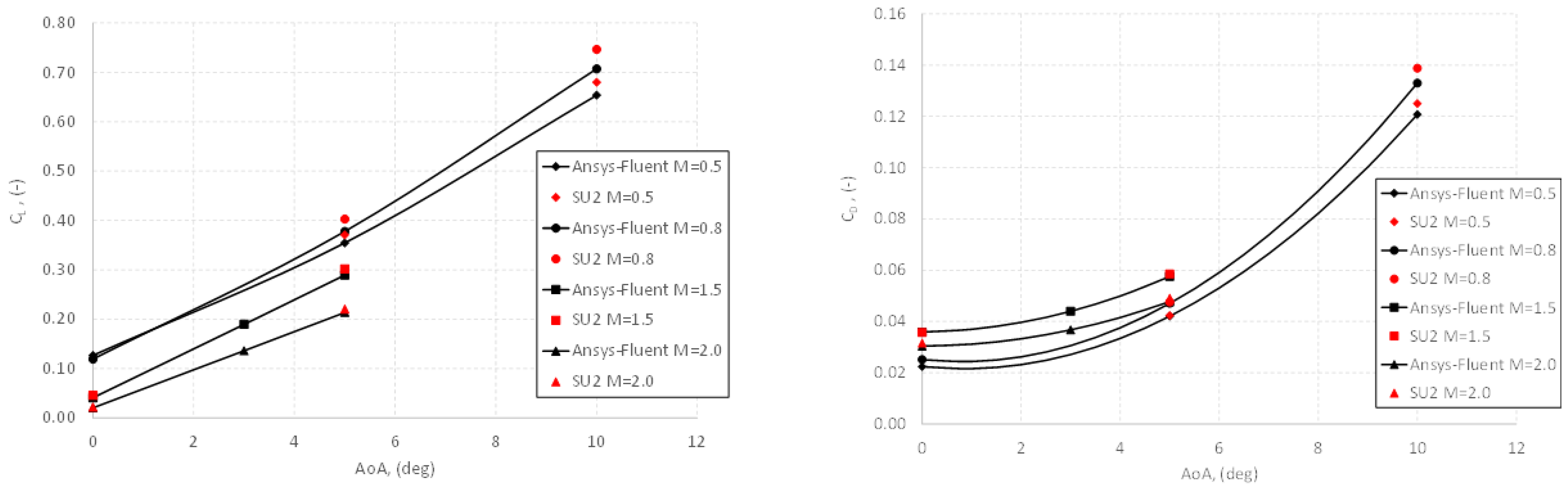
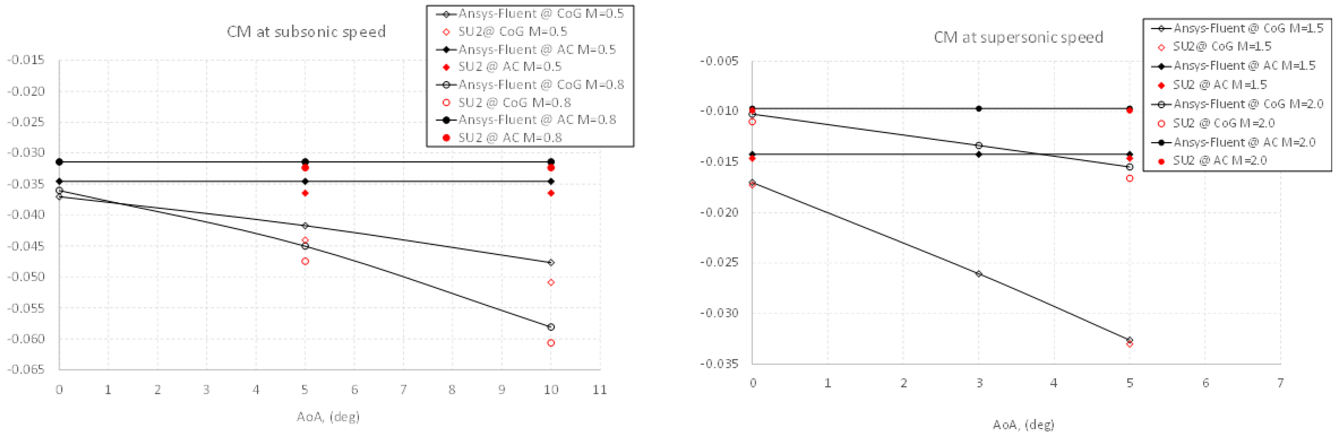
5.1. Force and Moment Coefficients Versus Attitude

The effect of aircraft attitude on its aerodynamic performances is summarized in Figure 10, where trends of the C L α and C D α curves for the different simulated Mach numbers are shown. Figure 10 also addresses the effect of numerical discretization of the SU2 solver versus the ANSYS-FLUENT solver. This comparison indicates that on the selected grid resolution, negligible differences between aerodynamic coefficients can be observed. This trend remains valid varying the Mach number and the AoA.
As one can see, in Figure 10 it is shown a quite satisfying match between the two codes for each simulated AoA. The flow physics appears correctly predicted by both the solvers. In fact, a quite linear and quadratic increase of C L and C D at intermediate AoA can be respectively observed without deviation from the expected trends. Recall that the non-linearity induced by the vortex lift phenomenon is expected to appear starting around about 10 deg AoA [24]. The above satisfying comparisons are also confirmed by the other aerodynamic data annotated in Table A1 and Table A2. However, looking at the C D coefficients, SU2 results appear to be over predicting the drag. To the best of authors experience, for simulations performed on complex aircraft configurations at the same Reynolds number, a larger difference (about over 50 drag counts) for SU2 with respect to a second order upwind scheme (like ROE FDS) suggests an over-diffusive behaviour due to current JST scheme in SU2 [30].
As far as the pitching moment coefficient is concerned, the behaviour of C M at different angles of attack and for M = 0.5 , 0.8 , 1.5 , and 2.0 is displayed in Figure 11. Two pole positions, namely the aircraft CoG and AC, are considered to compute C M . Positions chosen for the aircraft CoG at the considered Mach numbers are equal to 53.54 % , 54.38 % , 57.74 % , and 59.12 % of the wing root chord, respectively.
As shown, the evaluation of C M with respect to the AC clearly shows that the pitching moment does not depend on the AoA, as expected. Additionally, if the aircraft CoG is considered as pole, a quite linear trend for the C M is predicted, especially for supersonic speeds. For each Mach number, it can be further observed that the slope of C m α curve is negative. Therefore it is confirmed that the aircraft is statically stable, for all the simulated flight conditions, see also Table A1 Table A2. Finally, it is worth noting that a detailed description of the low-speed aerodynamics of this aeroshape can be found in Ref. [24].

5.2. Force and Moment Coefficients Versus Mach

As far as the effect of M on aircraft aerodynamic is concerned, in Figure 12 the Mach number contours fields at M = 0.5 , 0.8 , 1.5 , and 2.0 . are reported.Those contours are provided in the aircraft symmetry plane.
At M = 0.50, the effective lifting region is mainly located near the middle of the wing. Further, the sharp-induced leading edge separation with the consequent vortex roll-up provided by delta-wing planform creates, when the aircraft flies at moderate-high AoA, an increased suction on the leeside, according to the vortex lift phenomenon [22,25,38].
The low-pressure distribution due to the vortex lift is evident in Figure 13 left side, where primary and secondary vortex cores appears over the lee-side. These vortices can be also observed by looking at the skin friction lines reported on the aircraft leeside in Figure 13 right side. Further details on aircraft low-speed aerodynamics can be found in Ref. [24].
As far as M increases up to value M = 0.8 (transonic), the lifting region of the wing reduces. Therefore, at M = 0.8 the AC is expected to shift backward with respect to M = 0.5 , with the consequent increase of the static margin.
Consequently, the suction effect on the wing decreases, as shown in Figure 14.
At M = 1.5 , supersonic flow adapts on solid walls through an oblique shock waves systems and surface pressure distributions on both aircraft leeside and windside can be appreciated in Figure 15 for α = 5 .
The shock-shock interaction between the nacelles and the tails can be well observed. At supersonic Mach number appear visible the shockwave train which features the typical N-shaped pressure signature, which is responsible of the sonic boom. This is further significant as far as the Mach number is increased to higher supersonic values, see Figure 16.
By further increasing the Mach number up to M = 2.0 , the AC stabilises at about the 60 % of the root chord length.
Figure 16 depicts clearly the surface pressure distribution over the aircraft aerospace for α = 3 . A significant shocks system at nacelle intake is clearly recognizable.
Above flow-field evolution results in a corresponding variation of aerodynamic characteristics of the aircraft versus Mach Number, as summarized in Figure 17. It shows the behaviour of the lift, drag, lift-to-drag ratio, and pitching moment coefficients with respect to the AC as function of Mach number at α = 0 and α = 5 , respectively.
As one can see, aircraft aerodynamic characteristics are subjected to the compressibility crisis, that is clearly inferred form the rapid variations of force and moment coefficients around M = 1 . As the aircraft approaches the speed of sound, the flowfield past the vehicle is characterized by the presence of shock waves.
In particular, a discontinuity surface appears located just at the aircraft nose. Therefore, the oncoming airflow is abruptly deflected away from the aircraft surface and not flow smoothly around it. As a result, aerodynamic forces and moments change from those experienced at low incompressible flow conditions.
Aircraft drag sharply rises, starting from the drag divergence Mach number, due to the wave drag. For the above mentioned reasons, the drag coefficient of the aircraft close to sonic speed is greater than in the supersonic range due to the erratic shock formation and general flow instabilities, typical of flow field around M = 1 . But, once the supersonic flow establishes again, flow stabilises and the drag coefficient reduces.
Introducing the AC, which simplifies the dependence on the AoA of the moment reduction pole, the distance between the CoG and the AC (i.e., the static margin), determines the longitudinal static stability of the aircraft.
The above mentioned trend agrees with the backward shift of the AC towards the trailing edge, which is addressed in Table 2.
In this table, the dimensionless position of the aircraft AC (i.e., X ¯ A C ) is summarized at all investigated Mach numbers. The comparison between ANSYS-FLUENT and SU2 is also reported for M = 0.5 , 0.8 , 1.5 , and 2.0 .
The similitude of present aircraft wing planform and that of Concorde suggested to compare results in Table 2 with those available in literature for the X ¯ A C of the Concorde [26]. This comparison is provided in Figure 18 for the whole Mach number range.
As one can see, CFD results agree rather well with the Concorde data, with the higher difference obtained around M = 1.5 . According to Equation (14), the motivation of these discrepancies can be found looking at the variation of the axial and normal force coefficients versus Mach, shown in Figure 19. In this figure, profiles of C A and C N are shown versus M ranging from 1.02 to 2.00 and for both α = 0 d e g and 5 d e g . As one can see, both axial and normal coefficients increase starting from M = 1.10 , thus determining the larger shift of the aircraft AC, shown in Figure 18.
Finally, it is worth noting that the behaviour of C A and C N versus Mach is the result of the shocks train shift that takes place on the aircraft belly side and close to the engine nacelles as M increases, as can be recognized looking at the Mach contours in Figure 12 and at the pressure distributions from Figure 13, Figure 14, Figure 15 and Figure 16.

6. Conclusions

In the present paper, the longitudinal aerodynamic performance and the static stability of a Concorde-like aeroshape, conditioned to a large Mach number variation, were addressed using Computational Fluid Dynamics. Particular attention was focused on the shift of the aeroshape aerodynamic center to verify that the provided wing design allows the aircraft static margin to be within 5% of the reference length, both at low-speed and high-speed flight conditions. A set of very different flight conditions, encompassing the transition from subsonic to supersonic flight, was considered to describe the shift phenomenon of the aircraft aerodynamic centre, typical of supersonic aircraft. The aerodynamic force and moment coefficients of the aircraft were computed with two different CFD solvers, namely ANSYS-FLUENT and SU2, and results compared in order to gain prior knowledge over the accuracy of the solution over the whole flight envelope.
Result comparisons highlighted a satisfying match between the two codes for each simulated Mach and angle of attack. The flow physics appears correctly predicted by both the solvers. In fact, a quite linear and quadratic increase of C L and C D at different attitude conditions can be respectively observed without deviation from the expected trends. The computed pressure and Mach number contours revealed the correct evolution of the flow field predicted past the aircraft in the transition between the low-speed and high-speed regime. The shift of the aerodynamic centre at various Mach numbers was addressed and compared to literature data available for the Concorde, since the similarity of the investigated aeroshape to that of the first civilian supersonic aircraft. Numerical results agreed rather well with the Concorde data even though some differences were marked around M = 1.5 . Further investigations pointed out that these discrepancies were due to the variation of the axial and normal force coefficients versus Mach. Indeed, both axial and normal coefficients increase starting from M = 1.10 , thus determining a larger shift of the aircraft aerodynamic center. Finally, it is worth noting that the behaviour of axial and normal force coefficients versus Mach is the result of the shocks train shift that takes place on the aircraft belly side and close to the engine nacelles as M increases. Therefore, CFD results suggested to refine wing design, especially engine nacelles positions in order to guarantee that the aircraft static margin be within 5% of the moment reference length.
Simulations also shown that on the wide range of Mach number considered, a sensible difference of computed drag coefficients for SU2 solver was observed. Such a behaviour was explained by considering the grid resolution adopted, and the artificial diffusion involved in the computation of inviscid terms. Furthermore, the consistence of numerical results obtained with JST scheme implemented in SU2, confirmed that it can be used for a wide range of Mach number provided an adequate choice for dissipation operators. The same results was not confirmed for the upwind schemes currently implemented in SU2.
Finally, it is worth noting that the present work adds further results to the aerodynamic design of high-speed aircraft. In particular, the present paper addresses further investigations carried out also to consolidate in-house design capability for the development of highly aerodynamic efficient supersonic aircraft for civilian transportation. As further comment, although some differences appear for the computation of drag coefficient, SU2 is capable to predict the correct shift of the aerodynamic centre at varying Mach numbers. This represents a further contribution to the possibility offered by open-source platforms for future aerodynamic simulations of supersonic aircraft. These responses allow a rapid follow-up useful to researcher and engineers in conceptual design phase of supersonic aircraft.

Author Contributions

Conceptualization, G.P.; methodology and software, O.D.; A.A.; G.P.; validation, G.P.; A.A.; formal analysis, G.P., A.A.; resources, A.V.; data curation, G.P., O.D.; writing, A.A., G.P.; writing and editing, A.A., G.P.; review, A.V.; supervision, G.P. All authors have read and agreed to the published version of the manuscript.

Funding

This research received no external funding.

Conflicts of Interest

The authors declare no conflict of interest.

Appendix A

Appendix A.1

Aerodynamic coefficients for the simulated flight conditions obtained with Ansys-Fluent and SU2 codes. Clean configuration.
Table A1. CFD results in terms of aerodynamic force and moment coefficients. Ansys-Fluent code. Clean configuration.
M AoA C A C N C M nose C Mac C D C L L D
( ) ( deg ) ( ) ( ) ( ) ( ) ( ) ( ) ( )
0.2400.022780.12510−0.18960−0.034810.022800.125105.48684
0.2450.010420.35050−0.47730−0.034810.040800.347308.51225
0.24100.004380.65710−0.86720−0.034810.118400.646405.45946
0.5000.022380.12677−0.19272−0.034560.022380.126775.66494
0.5050.011010.35684−0.47995−0.034560.042070.354528.42631
0.50100.005430.66480−0.86412−0.034560.120790.653765.41237
0.8000.025100.11926−0.18349−0.031420.025100.119264.75083
0.8050.013940.38045−0.51544−0.031420.047040.377798.03108
0.80100.008130.71955−0.94782−0.031420.132960.707215.31897
0.9000.029430.11126−0.17347−0.030080.029430.111263.78045
0.9050.018770.39781−0.54273−0.030080.053370.394667.39439
0.9500.033970.10616−0.16827−0.029130.033970.106163.12474
0.9550.024980.40919−0.56493−0.029130.060550.405466.69619
1.0200.041320.08010−0.13016−0.023050.041320.080101.9384
1.0250.032700.41104−0.57253−0.023050.068400.406335.94493
1.1000.040040.07630−0.12145−0.019290.040040.076301.9554
1.1050.031360.38857−0.53941−0.019290.065110.384365.90311
1.2000.039310.07512−0.12012−0.020480.039310.075121.91121
1.2050.031680.36445−0.50491−0.020480.063320.360305.68984
1.5000.035670.04353−0.07230−0.014230.035870.040861.13923
1.5030.033970.19165−0.26948−0.014230.043960.189614.31344
1.5050.031890.29632−0.40898−0.014230.057530.289465.03137
1.8000.032230.02413−0.04252−0.010660.032230.020470.74872
1.8050.030040.24066−0.32823−0.010660.050900.237134.65908
2.0000.030380.02047−0.03653−0.009700.030380.020470.67398
2.0030.029500.13798−0.19051−0.009790.036680.136253.71415
2.0050.028870.21709−0.29420−0.009700.047680.213754.48329
Table A2. CFD results in terms of aerodynamic force and moment coefficients. SU2 code. Clean configuration.
M AoA C A C N C M nose C Mac C D C L L D
( ) ( deg ) ( ) ( ) ( ) ( ) ( ) ( ) ( )
0.550.009810.37316−0.51314−0.036450.042300.370888.76763
0.5100.005020.69145−0.92005−0.036450.125020.680075.43959
0.850.012300.40531−0.56036−0.032340.047580.402708.46338
0.8100.007030.75923−1.0214−0.032340.138770.746485.37923
1.500.035680.04559−0.0765−0.014630.035680.045591.27776
1.550.031970.30584−0.4292−0.014630.058500.301895.15974
2.000.031500.02188−0.0388−0.009900.031500.021880.69462
2.050.029700.22400−0.30400−0.009900.049110.220564.49114

References

  1. Carioscia, S.A.; Locke, J.W.; Boyd, L.D.; Lewis, M.J.; HalionSun, R.P.; Smith, H. Commercial Decelopment of Civilian Supersonic Aircraft; Coument D-10845; IDA: Alexandria, VA, USA, 2019. [Google Scholar]
  2. Sun, Y.; Smith, H. Review and prospect of supersonic business jet design. Prog. Aerosp. Sci. 2017, 90, 12–38. [Google Scholar] [CrossRef]
  3. Liebhardt, B.K. An Analysis of the Market Environment for Supersonic Business Jets. Prog. Aerosp. Sci. 2011, 39, 185–248. [Google Scholar]
  4. Davies, R.E.G. Supersonic (Airliner) Non-Sense—A Case Study in Applied Market Research; Coument D-10845; IDA: Alexandria, VA, USA, 1998. [Google Scholar]
  5. Smith, H. A review of supersonic business jet design issues. Aeronaut. J. 2007, 111, 761–764. [Google Scholar] [CrossRef]
  6. Smith, H. Supersonic Experimental Airplane (NEXST) for Next Generation SST Technology-Development and flight test plan for the Unmanned Scaled Supersonic Glider. In Proceedings of the AIAA-2002-0527. 39th Aerospace Sciences Meeting & Exhibit, Reno, NV, USA, 8–11 January 2001; pp. 761–764. [Google Scholar]
  7. Henne, P.A. Case for Small Supersonic Civil Aircraft. J. Aircr. 2005, 39, 765–774. [Google Scholar] [CrossRef]
  8. Sun, Y.; Smith, H.; Chen, H. Conceptual design of Low-Boom Low-Drag Supersonic Transports. In Proceedings of the AIAA Aviation Forum, 15–19 June 2020; Virtual Event. [Google Scholar]
  9. Aerion Supersonic. 2017. Available online: https://www.aerionsupersonic.com (accessed on 16 July 2022).
  10. Spike Aerospace. 2021. Available online: https://www.spikeaerospace.com/spike-images/ (accessed on 16 July 2022).
  11. Boom Airliner. Available online: https://boomsupersonic.com/airliner (accessed on 16 July 2022).
  12. Hardeman, A.B.; Maurice, L.Q. Sustainability:key to enable next generation supersonic passenger flight. In Proceedings of the IOP Conference Series: Materials Science and Engineering, Sanya, China, 12–14 November 2021. [Google Scholar]
  13. Lee, D.S.; Fahey, D.W.; Forster, P.M.; Newton, P.J.; Wit, R.C.; Owen, B.; Sausen, R. Aviation and global climate change in the 21st century. Atmos. Environ. 2009, 43, 3520–3537. [Google Scholar] [CrossRef]
  14. Feng, X.; Li, Z.; Song, B. Research of low boom and low drag supersonic aircraft design. Chin. J. Aeronaut. 2014, 27, 531–541. [Google Scholar]
  15. Choi, S.; Alonso, J.J.; Kroo, I.; Wintzer, M. Multi-fidelity design optimization of low boom supersonic jets. J. Aircr. 2008, 45, 106–118. [Google Scholar] [CrossRef]
  16. Takeshi, F.; Yoshikazu, M. Conceptual design and aerodynamic optimization of silent supersonic aircraft at JAXA. In Proceedings of the 25th AIAA Applied Aerodynamics Conference, Miami, FL, USA, 25–28 June 2007. [Google Scholar]
  17. Sun, Y.; Smith, H. Low-boom low-drag optimization in a multidisciplinary design analysis optimization environment. Aerosp. Sci. Technol. 2019, 94, 105387. [Google Scholar] [CrossRef]
  18. Sun, Y.; Smith, H. Design and operational assessment of a low-boom low-drag supersonic business jet. Proc. Inst. Mech. Eng. Part J. Aerosp. Eng. 2022, 236, 82–95. [Google Scholar] [CrossRef]
  19. Yoshida, K. Supersonic drag reduction technology in the scaled supersonic experimental airplane project by JAXA. Prog. Aerosp. Sci. 2009, 45, 124–146. [Google Scholar] [CrossRef]
  20. Mangano, M.; Martins, J.R. Multipoint aerodynamic optimization for subsonic and supersonic regimes. J. Aircr. 2021, 58, 650–662. [Google Scholar] [CrossRef]
  21. Seraj, S.; Martins, J.R.R.A. Aerodynamic shape optimization of a supersonic transport considering low-speed stability. In Proceedings of the AIAA Scitech 2022 Forum, San Diego, CA, USA, 3–7 January 2022. [Google Scholar]
  22. Gursul, Z.W.I.; Vardaki, E. Review of flow control mechanisms of leading-edge vortices. Prog. Aerosp. Sci. 2007, 43, 246–270. [Google Scholar] [CrossRef]
  23. Gursul, I. Review of unsteady vortex flow over delta wings. J. Aircr. 2005, 42, 299–319. [Google Scholar] [CrossRef]
  24. Aprovitola, A.; Di Nuzzo, P.E.; Pezzella, G.; Viviani, A. Aerodynamic Analysis of a Supersonic Transport Aircraft at Landing Speed Conditions. Energies 2021, 14, 6615. [Google Scholar] [CrossRef]
  25. Luckring, J. The discovery and prediction of vortex flow aerodynamics. Aeronaut. J. 2019, 123, 729–804. [Google Scholar] [CrossRef]
  26. Rech, J.; Leyman, C. A Case Study by Aerospatiale and British Aerospace on the Concorde. AIAA Prof. Study Ser. 1980. [Google Scholar] [CrossRef]
  27. Eames, J.D. Concorde Operations. SAE Trans. J. Aerosp. 1991, 100 Pt 2, 2603–2619. [Google Scholar]
  28. Krus, P.; Abdallah, A. Modelling of Transonic and Supersonic Aerodynamics for Conceptual Design and Flight Simulation. In Proceedings of the Aerospace Technology Congress, Stockholm, Sweden, 8–9 October 2019; Swedish Society of Aeronautics and Astronautics (FTF): Stockholm, Sweden, 2019. [Google Scholar]
  29. British Airways Overseas Division. Concorde Flying Manual II a; British Airways: London, UK, 1977. [Google Scholar]
  30. Aprovitola, A.; Aurisicchio, F.; Di Nuzzo, P.E.; Pezzella, G.; Viviani, A. Low Speed Aerodynamic Analysis of the N2A Hybrid Wing—Body. Aerospace 2022, 9, 89. [Google Scholar] [CrossRef]
  31. Bykerk, T.; Pezzella, G.; Verstraete, D.; Viviani, A. Longitudinal And Lateral-Directional Aerodynamics of a Re-Usable High-Speed Vehicle. In Proceedings of the 32nd Congress of the International Council of the Aeronautical Sciences, Shanghai, China, 6–10 September 2021. [Google Scholar]
  32. Schettino, A.; Pezzella, G.; Marini, M.; Di Benedetto, S.; Villace, V.F.; Steelant, J.; Choudhury, R.; Gubanov, A.; Voevodenko, N. Aerodynamic database of the HEXAFLY-INT hypersonic glider. CEAS Space J. 2020, 12, 295–311. [Google Scholar] [CrossRef]
  33. ANSYS-FLUENT. Ansys Fluent User’s Guide; ANSYS-FLUENT: Canonsburg, PA, USA, 2019. [Google Scholar]
  34. Economon, T.; Palacios, F.; Copeland, S.; Lukaczyck, T.; Alonso, J. SU2: An Open-SOurce suite for multiphysics simulation and design. AIAA J. 2016, 54, 828–846. [Google Scholar] [CrossRef]
  35. van Leer, B.; Powell, K. Introduction to Computational Fluid Dynamics. In Encyclopedia of Aerospace Engineering; John Wiley & Sons, Ltd.: Hoboken, NJ, USA, 2010. [Google Scholar]
  36. Jameson, A. Origins and further development of the Jameson-Smith-Turkel scheme. AIAA J. 2017, 55. [Google Scholar] [CrossRef]
  37. Hirsh, C. Numerical Computation of Internal and External Flow; Butterworth-Heinemann: Oxford, UK, 2007. [Google Scholar]
  38. Ekaterinaris, J.A.; Schiff, L.B. Numerical simulation of incidence and sweeep effects on delta wing vortex breakdown. J. Aircr. 1994, 31, 1043–1049. [Google Scholar] [CrossRef]
Figure 1. The aircraft configuration with dimensions.
Aerospace 09 00411 g001
Figure 2. Design parameters of the aircraft configuration.
Aerospace 09 00411 g002
Figure 3. The Concorde flight envelope in the altitude-airspeed plane with iso-Mach lines [26,29].
Aerospace 09 00411 g003
Figure 4. Subsonic computational domain with mesh on the aircraft wall and symmetry plane.
Aerospace 09 00411 g004
Figure 5. Supersonic computational domain with mesh on the aircraft wall and symmetry plane.
Aerospace 09 00411 g005
Figure 6. Typical boundary layer prismatic cells with mesh on the aircraft wall and symmetry plane.
Aerospace 09 00411 g006
Figure 7. Body ( X B , Y B , Z B ) and Wind ( X W , Y W , Z W ) reference frames with aerodynamic force and moment coefficients.
Aerospace 09 00411 g007
Figure 8. Aircraft root chord dimension and wing leading edge position with respect to the nose.
Aerospace 09 00411 g008
Figure 9. Pitching moment coefficient versus α and for different positions of the pole reduction point along with the wing Root Chord (RC) for M = 2.0 and R e L r e f = 1.01 × 10 8 .
Aerospace 09 00411 g009
Figure 10. Lift and drag coefficients versus α . Comparison between ANSYS-FLUENT and SU2 for M = 0.5 , 0.8 , 1.5 , and 2.0 .
Aerospace 09 00411 g010
Figure 11. Pitching moment coefficients versus α . Comparison between ANSYS-FLUENT and SU2 for M = 0.5 , 0.8 , 1.5 , and 2.0 .
Aerospace 09 00411 g011
Figure 12. Mach contours at M = 0.5, 0.8, 1.5, and 2.0 and for α = 0 .
Aerospace 09 00411 g012
Figure 13. Pressure contours and surface streamlines at M = 0.5 and α = 10 .
Aerospace 09 00411 g013
Figure 14. Pressure contours at M = 0.8 and α = 5 .
Aerospace 09 00411 g014
Figure 15. Pressure contours at M = 1.5 and α = 5 .
Aerospace 09 00411 g015
Figure 16. Pressure contours at M = 2.0 and α = 3 .
Aerospace 09 00411 g016
Figure 17. Force and moment coefficients versus M . Comparison between Ansys-Fluent and SU2.
Aerospace 09 00411 g017
Figure 18. Shift of aerodynamic center with Mach number: Concorde literature data (solid line), CFD results (dotted data) [26].
Aerospace 09 00411 g018
Figure 19. Axial and normal force coefficients versus M in supersonic flow conditions.
Aerospace 09 00411 g019
Table 1. CFD Test matrix.
M Re L ref / 10 8 α AltitudePressureTemperature
( ) ( ) ( deg ) ( km ) ( Pa ) ( K )
0.241.6000.030100,965.40287.95
0.241.6050.030100,965.40287.95
0.241.60100.030100,965.40287.95
0.503.1200.34997,202.10285.88
0.503.1250.34997,202.10285.88
0.503.12100.34997,202.10285.88
0.803.1805.09053,402.00255.09
0.803.1855.09053,402.00255.09
0.803.18105.09053,402.00255.09
0.902.9107.08040,645.40242.13
0.902.9157.08040.645.40242.13
0.952.8107.94035,961.00236.60
0.952.8157.94035,961.00236.60
1.022.8107.94035,961.00236.60
1.022.8157.94035,961.00236.60
1.102.56010.07026,154.20222.70
1.102.56510.07026,154.20222.70
1.202.61010.66023,872.10218.86
1.202.61510.66023,872.10218.86
1.501.01018.2887231.20216.65
1.501.01318.2887231.20216.65
1.501.01518.2887231.20216.65
1.801.01018.2887231.20216.65
1.801.01518.2887231.20216.65
2.001.01018.2887231.20216.65
2.001.01318.2887231.20216.65
2.001.01518.2887231.20216.65
Table 2. Position of the aerodynamic center: comparison between ANSYS-FLUENT and SU2.
X ¯ AC
M ANSYS-FLUENTSU2
0.240.5490-
0.500.55520.539
0.800.58080.584
0.900.5960-
0.950.6170-
1.020.6440-
1.100.6460-
1.200.6360-
1.500.63950.637
1.800.6270-
2.000.61780.616
Publisher’s Note: MDPI stays neutral with regard to jurisdictional claims in published maps and institutional affiliations.

