
Layout Analysis and Optimization of Airships with Thrust-Based Stability Augmentation


Dipartimento di Scienze e Tecnologie Aerospaziali, Politecnico di Milano, Via La Masa 34, 20156 Milan, Italy
*
Author to whom correspondence should be addressed.
†
These authors contributed equally to this work.
Aerospace 2022, 9(7), 393; https://doi.org/10.3390/aerospace9070393
Submission received: 28 June 2022
/
Revised: 15 July 2022
/
Accepted: 16 July 2022
/
Published: 21 July 2022
(This article belongs to the Special Issue Mission Analysis and Design of Lighter-than-Air Flying Vehicles)
Abstract
:Despite offering often significant advantages with respect to other flying machines, especially in terms of flight endurance, airships are typically harder to control. Technological solutions borrowed from the realm of shipbuilding, such as bow thrusters, have been largely experimented with to the extent of increasing maneuverability. More recently, also thrust vectoring has appeared as an effective solution to ameliorate maneuverability. However, with an increasing interest for high-altitude airships (HAAs) and autonomous flight and the ensuing need to reduce weight and lifting performance, design simplicity is a desirable goal. Besides saving weight, it would reduce complexity and increase time between overhauls, in turn enabling longer missions. In this perspective, an airship layout based on a set of non-tilting thrusters, optimally placed to be employed for both propulsion and attitude control, appears particularly interesting. If sufficiently effective, such configurations would reduce the need for control surfaces on aerodynamic empennages and the corresponding actuators. Clearly, from an airship design perspective, the adoption of many smaller thrusters instead of a few larger ones allows a potentially significant departure from more classical airship layouts. Where on one side attractive, this solution unlocks a number of design variables—for instance, the number of thrusters, as well as their positioning in the general layout, mutual tilt angles, etc.—to be set according simultaneously to propulsion and attitude control goals. In this paper, we explore the effect of a set of configuration parameters defining three-thrusters and four-thrusters layout, trying to capture their impact on an aggregated measure of control performance. To this aim, at first a stability augmentation system (SAS) is designed so as to stabilize the airship making use of thrusters instead of aerodynamic surfaces. Then a non-linear model of the airship is employed to test the airship in a set of virtual simulation scenarios. The analysis is carried out in a parameterized fashion, changing the values of configuration parameters pertaining to the thrusters layout so as to understand their respective effects. In a later stage, the choice of the optimal design values (i.e., the optimal layout) related to the thrusters is demanded to an optimizer. The paper is concluded by showing the results on a complete numerical test case, drawing conclusions on the relevance of certain design parameters on the considered performance, and commenting the features of an optimal configuration.
1. Introduction
In recent times, airships have regained the interest of researchers and engineers, as potentially advantageous solutions for carrying out different types of missions. These include primarily high-altitude pseudo-satellites (HAPS). The design of high-altitude airships (HAAs) has been in the focus of several research endeavors [1,2,3,4,5,6,7,8], which due to the relative immaturity of design techniques specifically targeting this mission, mostly consider preliminary design. They consequently focus on understanding the general features of an airship for such mission, such as weight, installed power, volume, shape, area of solar cells, etc. Despite reaching in some instances the prototype stage (as is the case for the HiSentinel series and Hale-D in the United States or YuanMeng in China), existing HAAs are typically proofs of concept, featuring a relatively standard overall layout, compared to older airships.
The latter is also generally the case for the most recent design studies and applications in the field of low altitude flights, where airships are gaining industrial interest as alternatives to unmanned multi-copters [9,10,11,12,13].
Over the last decade, the application of novel propulsion concepts in aeronautics has been focusing particularly on the inclusion of an electric component in the power-train [14,15,16,17], and related enabling technologies [18]. On airships, the adoption of electric motors, to drive the propellers instead of piston-powered units, allows benefiting from more compact and simpler thrusters. Conjugated with solar cells, such thrusters may be fed for long periods of time especially when considering HAPS missions, at altitudes where the solar incident radiation is higher. As highlighted in some studies [3,4], corresponding HAAs may take on missions spanning several weeks at once. Therefore, the limit to even higher flight times would be attributed to other issues, including overhauling of the payload and of the airship plants (as practically observed in the case of the HiSentinel campaign). The latter would be decreased in the most effective way by pushing on design simplicity, i.e., removing movable parts and the corresponding actuators as much as possible.
One such design simplification may be obtained by suppressing movable control surfaces, exploiting the adoption of more electric thrusters for control. Of course, due to the generally marginal stability characteristics of airships, the artificial stability augmentation typically on-board would be demanded to the thrusters, which would be employed simultaneously to push the aircraft in forward flight (or station-keeping against a constant wind for HAAs in HAPS missions), maneuvers, and to stabilize the system in presence of disturbances.
A very effective, solution in this sense comes from thrust vectoring, which has been employed also on some of the few airships currently flying regularly (e.g., Zeppelin LZ N07-101).
However, to the aim of increasing simplicity, a smart placement (i.e., layout) of the thrusters onboard would be possibly a more promising solution. On the other hand, the placement of thrusters would be also a more delicate task, since it should answer the need for several propulsion and control goals at once, as pointed out. Furthermore, the assignment of a configuration requires the definition of a relatively large set of geometric parameters, including the three-dimensional positioning of the thrusters with respect to the hull (as well as with respect to the buoyancy center and center of gravity), the tilt angle of the thrusters, and clearly their number. This makes the analysis and the selection of an optimal configuration a potentially challenging problem [8,19].
In the present paper, we try to explore this design problem. Taking inspiration from existing airship layouts, a baseline airship featuring a cruciform, tailback configuration with movable surfaces, and a single pushing thruster, is selected. The baseline layout is altered, making computations assuming to remove the existing thruster and replacing it with three or four thrusters in multiple layouts. In particular, free design parameters include the three-dimensional positioning of all thrusters with respect to the buoyancy center of the hull, as well as the fixed vertical tilt angle of the thrusters with respect to the longitudinal axis. In order to stabilize the system, a stability augmentation system (SAS) is designed and implemented, taking as inputs rates usually measurable on flying vehicles, and producing as outputs stabilizing values of the thrust settings.
In order to synthetically capture the performance of a certain layout and allow mutual comparisons, a cost function sensible to both the departure from a trimmed condition and the energy required by the actuators to control the airship is defined. A non-linear model of the airship is introduced, which is originally implemented and subject to the mentioned purpose-designed control laws, integrating forward-in-time its behavior starting from perturbations of trimmed, horizontal flight conditions. The action of the SAS is such to restore trimmed flight, with a performance which is the direct result of a choice of the layout.
A parameter analysis is carried out first to preliminarily map the cost function just introduced and to assess its sensitivity to the assumed design parameters (i.e., geometric quantities defining the layout of the thrusters configurations).
Finally, an optimization algorithm is deployed to automatically find the optimal configuration, minimizing the selected cost function. A comparison of results in significant scenarios is proposed, trying to understand the dependence of the optimal solution on trim airspeed as well as geometric features of the layout. Finally, exploiting the nature of the proposed cost function, an assessment of the relative advantage of a thruster layout with respect to another is attempted.
2. Dynamic Model of the Airship
In order to ease the comparison between different layouts of the thrusters, the formulation for the dynamics of the airship has been written in an agnostic form, according to a vectorial formalism. Considering the dynamic equilibrium for displacement and rotational motion, the generalized vector form is assumed, yielding the following:
![Aerospace 09 00393 i002]() where generalized mass matrix is a function of the mass m, static moment , and moment of inertia , which are arranged as follows.
where generalized mass matrix is a function of the mass m, static moment , and moment of inertia , which are arranged as follows.

In Equation (1) the generalized velocity vector is , i.e., listing, respectively, the velocity of the generic point with respect to an inertial observer, and the rotational speed of the airship body with respect to the same observer. The southwest product operator ![Aerospace 09 00393 i001]() applied to yields the following.
applied to yields the following.
![Aerospace 09 00393 i003]()
 applied to yields the following.

The generalized forcing term in Equation (1) is defined as , where the two components represent, respectively, the resultants of the force and moment (the latter with respect to the measuring point ) due to aerodynamics (), buoyancy (), gravity (), and propulsion ().
In order to make Equation (1) explicit, a body reference system is chosen (indicated with ), centered in the center of buoyancy , with the first axis pointing to the nose of the airship, the third to the bottom, and consequently the second to the right. The two systems are shown in a sketch in Figure 1. With respect to an inertial reference on the ground (indicated with ), it is possible to obtain the body reference from the ground one via a rotation tensor , where , , and are angular parameters, physically interpreted as attitude angles of roll, pitch, and yaw, respectively [20].
The generalized mass in Equation (2) will be localized in the center of buoyancy, according to the choice . It is noteworthy that the static moment is not identically null (unlike in typical winged aircraft dynamics applications), since the reference point is not in the center of gravity . In body reference, the components of the speed vector take the scalar definitions , whereas the components of the rotational speed . Consequently, the inertial part (i.e., the left hand side) of dynamic equilibrium in Equation (1) will produce six scalar expressions, functions of inertia components in the body frame, and the six scalar kinematic variables just introduced (and their first-order time derivatives).
By components in the body frame , the forcing term on the right hand side of Equation (1) can be written as described next.
2.1. Aerodynamics
An aerodynamic model allowing a balance of accuracy and simplicity deemed suitable for the present study, centered on flight dynamics, has been described in [21,22,23]. The contribution can be split into two components, an active term similar to most winged flying vehicles , and a reaction term due to the displacement of surrounding air by action of the hull, called . By components in the body frame , the active term can be written according to the aircraft dynamics nomenclature [20], where the dependence of each component is modeled according to a first-order expansion with respect to the kinematic variables. Taking into account the mutual balance between coefficients for an airship with a standard hull and tail configuration and proportion, it is possible to reduce the number of parameters in the expansion, thus yielding for [22]:
The scalar sensitivities appearing in the first matrix on the right hand side of Equation (4) can be modeled via the Munk–DeLaurier theory [21,24], making use of the potential flow theory for the hull part, as well as of standard incompressible lifting surface aerodynamics for the empennages [20]. The corresponding modeling is a function of the specific geometry of the hull and fins. For the former, a detailed analytic description is required, usually attainable at least for axis-symmetric, regular shapes of the envelope. For tail lifting surfaces, methods for obtaining lumped force and moment coefficients for an assigned platform, span, and aerodynamic profile, originally developed for aircraft, still hold for the airship case. Corrections for the interaction between the envelope and tail surfaces allow an accurate mix of teh contributions of the two most aerodynamically relevant components of the airship [22].
In Equation (4), is the array of controls, and matrix modulates the effect of controls on the aerodynamic force. For standard airship steering and stability augmentation, based on the deflection of aerodynamic surfaces on the tail, this component will be a sparse non-zero matrix, with coefficients modeled according to standard methods for deflectable surfaces, inherited from the winged aircraft case [20]. In this work, where thrust-based control is adopted and there are no deflectable (i.e., control) parts on the tail surfaces, the definition of the control term as applies, where each scalar represents the thrust setting of the corresponding thruster, and is the number of thrusters. Since the effect of this control is on propulsion force, in Equation (4) we have . The control vector, and the corresponding control action, will be modeled as part of the propulsion force (see later Section 2.3).
The reaction component of the aerodynamic forcing terms can be modeled according to a model making use of Munk’s shape-specific coefficients , , , and , and is proportional to the time rate of the generalized velocity [22]. In body components, for an axis-symmetric body of volume , this forcing term yields the following:
where is the density of air, and are diagonal components of , expressed in the body reference centered in . Since the term in Equation (5) is a function of the rate , it is typically moved to the left hand side of Equation (1) and treated as an additional mass term in dynamic equilibrium.
2.2. Buoyancy and Gravity
The term is composed of a non-null force term, and an identically null moment, since buoyancy acts by definition in the center of buoyancy . An expression of buoyancy force is particularly straightforward in the ground inertial reference, where it bears a single non-null component pointing up from the ground.
Similarly, gravity force bears an expression which is structurally close to that of buoyancy (i.e., a single component normal to the ground). However, since and are not in the same location, gravity exerts a non-null moment with respect to .
By components in the body reference, buoyancy, and gravity yield, we have the following:
where is the transpose of the matrix representation in either or of the rotation tensor , is the position vector of from in body components, and g is the modulus of gravitational acceleration.
It can be pointed out that gravity and buoyancy bring the additional variables wrapped in array as unknowns into the expression of dynamic equilibrium. This increase in the number of scalar unknowns in the formulation of dynamic equilibrium is balanced by invoking the kinematic equations relating to the body components of the rotational rate , yielding the following:
where matrix . This allows obtaining a balanced 9-by-9 system of first-order, non-linear differential equations, representing the dynamic equilibrium of the system.
2.3. Thrust
Total thrust force and moment around are obtained from the sum of the contributions of each of the thrusters. The thrust vector pertaining to the i-th thruster can be oriented with respect to the body reference through a swing angle and a tilt angle , according to Figure 2.
Therefore, the total force and moment in body reference components are as follows:
wherein is the representation in body components of the position vector pointing from to the point of application of , named . Intensity is expressed as a function of the control variable as follows:
where is the nominal value of thrust from the i-th thruster. The control modulates the nominal value through the shape function . The latter allows the reproduction of possible regime-dependent efficiency effects, or non-linear features related to the specific thruster technology. Furthermore, according to the technology implemented in the thruster, a different range of values can be considered. For instance, for a piston engine, this control would be limited to a positive value, whereas for electric motors or ion thrusters it may be also negative, thus producing an inversion of the thrust force, exploiting a well-known advantage of these types of thrusters with respect to more standard piston-powered ones.
It should be noted that the formulation just introduced through Equation (8) bends itself to the inclusion of thrust vectoring, which would require properly subordinating and to a control logic, instead of assigning them as geometrical parameters, as is of interest in this work.
3. Thrusters Layout and Thrust-Based Control
As stated in Section 1, in this paper the effect on the dynamic response of the airship sorted by the value assumed by a set of geometrical parameters is of interest. A shortlist of configurations of potential interest, for which quantitative design analyses will be performed, is formed mainly based on two drivers:
- Number of thrusters (). Where on the one hand it may be interesting to increase this number to achieve better controllability and investigate arbitrary configurations, in practice a higher number of thrusters would proportionately increase the chance of failure, and consequently system downtime. Together with a greater complexity of the control system which should be faced when dealing with an increasing number of control variables (i.e., thrust settings), a greater number of thrusters would likely increase also the cost of manufacture. Therefore, layouts with a low number of thrusters are preferred in this work.
- Positioning of thrusters. Even considering the equilibrium flight conditions most often encountered, i.e. straight horizontal flight at different airspeeds (which also includes station-keeping in constant stratospheric wind for a HAA), airships of standard back-tailed configuration are usually marginally dynamically stable or slightly unstable. In particular, recurring to a modal analysis in a linearized framework, carried out around a trimmed condition in straight, horizontal, steady flight, lateral-directional motion of airships is typically dynamically unstable (due to sideslip subsidence), and longitudinal motion may feature a low-damped pendulum oscillatory mode [22]. For conditioning the dynamics of the system and easing piloting, artificial stability can be obtained in forward flight (not in hover) by implementing a SAS acting on the tail control surfaces. When deleting the (movable) control surfaces, while leaving the tail as a purely passive (stabilizing) assembly, such artificial stability augmentation is delegated to the thrusters. Clearly, this puts constraints on the placement and orientation of the thrusters. For instance, two-thruster configurations would not be able to stabilize the system in terms of both longitudinal and lateral-directional dynamics. Furthermore, when all thrusters are aligned with the longitudinal body axis, no direct roll control could be achieved, despite retaining control abilities through the intrinsic yaw-roll aerodynamic coupling of the airship. Therefore, basic layouts for quantitative investigations need to be preliminarily checked in terms of their ability in principle to perform a control action around all airship body axes.
According to these two drivers, three thruster layouts have been considered in the present work—namely (A), (B), and (C)—which appear as compromises between simplicity and control authority. They are described in the sketches in Figure 3.
From a geometrical standpoint, all configurations share the same arrangement of the baseline airship less the thrusters—hull, tail empennages, and payload—and differ only for the number and positioning of the thrusters. From the viewpoint of inertia, the number and positioning of the thrusters in the layout imply a different positioning of the , and changing values of the overall mass, static, and inertia moment, i.e., virtually all components in Equation (2) shall be affected.
A description of the configurations presented in Figure 3 will be proposed next.
3.1. Description of Thruster Layouts
3.1.1. Features of Layout (A)
Layout (A) features a set of three thrusters, where #1 and #2 share the vertical body coordinate and are symmetrically placed with respect to the vertical plane of symmetry of the airship. Thruster #3 is located on the plane of symmetry.
Thrusters #1 and #2 feature a line of thrust passing below , whereas that of #3 passes above that point. This allows thrusters in this configuration to control the motion around the pitch axis. The laterally symmetric positioning of #1 and #2 allows yaw control. In order to achieve direct roll control, however, a non-null tilt of the couple #1 and #2 needs to be implemented. In this manner, a differential use of #1 and #2 thrusters would produce a torque around the roll axis. For instance, starting from a trimmed condition, and a small positive , i.e., thrusters pointing slightly downwards with respect to the longitudinal body axis, a small increase on #1 thrust and a corresponding decrease on #2 would introduce a negative rolling moment, which would not be achieved if the two tilt angles of the thrusters were null. Clearly, it can be observed that such differential action would produce also a yawing moment.
A down-tilt of #1 and #2 thrusters may be compensated by an up-tilt of #3, i.e., , to allow avoiding an increase in body vertical speed V as an effect of a homogeneous (i.e., not differential) action on #1 and #2—as in trimmed forward flight.
In principle, from a control standpoint, an opposite mutual setting of the thruster tilt may be hypothesized as well (namely and ), but considering the positioning of the thrusters towards the tailcone of the hull, that choice would point the thrusters towards the hull, which due to the aerodynamic flow around the latter would bear a counter-intuitive and uncommon configuration.
In this layout, of particular interest are the longitudinal positions of the thrusters, and , as well as the dihedral angle of #1 and #2 with respect to the horizontal. Moreover, the lengths and of the radii of the respective thrusters from the longitudinal body axis are also of interest.
Broadly speaking, configuration (A) can be expected to be the cheapest and simpler to design, as well as the least prone to propulsion fault thanks to the lowest possible number of thrusters, but also the one providing the least control effectiveness, making use of the shortest possible number of control degrees of freedom for stabilization around all body axes.
3.1.2. Features of Layout (B)
The second layout is intended to explore the baseline ‘+’-shaped cruciform configuration. Besides an increased number of thrusters with respect to (A), in layout (B) control in the longitudinal plane (i.e., around pitch axis) is delegated to the combined use of thrusters #3 and #4, whereas lateral-directional control is obtained through the differential use of thrusters #1 and #2. As observed for configuration (A), a down-tilt of #1 and #2 is needed to obtain direct roll control, to be compensated by an up-tilt of #3 (on account of a down-tilt of #4, according to the shape of the tailcone).
Quantities of interest in this configuration are the longitudinal positions , which is the same for #1 and #2 for lateral symmetry, as well as and . The position of thrusters #3 and #4 is on the vertical plane of symmetry, with a radius of and respectively from the longitudinal axis, whereas the lateral thrusters #1 and #2 can be at a dihedral angle from the horizontal body plane, which is a relaxation from a strictly ‘+’-shaped layout, and at a radius of from the longitudinal axis.
Configuration (B) may be likely more expensive than (A), due to the additional thruster, but artificial stabilization should be in principle easier to design, thanks to a possible decoupling between the longitudinal and lateral-directional action. It would be also possibly more effective, i.e., such to achieve a faster convergence following perturbation through a more limited action of the controls.
3.1.3. Features of Layout (C)
The third layout has been envisaged to explore the features of a ‘×’-shaped configuration of four thrusters. The couple of #1 and #2 thrusters is attached to the lower part of the airship, to the right and left respectively. Similarly, #3 and #4 are located on the top part of the airship, symmetrically with respect to the vertical plane of symmetry.
The geometry is defined by the longitudinal distances and of the corresponding thrusters from , by the radii and from the longitudinal axis, and by the dihedral angles and , which measure the angular distance respectively of the lower (#1 and #2) and upper (#3 and #4) thrusters from the horizontal body plane.
Similarly to the other cases, direct roll control can be implemented by setting proper values of and .
From a control standpoint, artificial stabilization around all body axes can be effectively achieved in this configuration. An increase in the thrust of (#1, #2) together with a decrease on (#3, #4) shall provide positive pitching moment and vice-versa. A decrease in (#1, #4) setting and a simultaneous increase in (#2, #3) shall provide a positive yawing moment, and vice-versa. Finally, for a down-tilted (#1, #2) and an up-tilted (#3, #4) couple, a positive rolling moment could be obtained in principle by only increasing (#1, #3) setting, and a negative rolling moment by increasing (#2, #4). However, a more effective roll control can be achieved by additionally decreasing (#2, #4) for a positive rolling moment, and (#1, #3) for a negative one.
3.2. Thrust-Based Artificial Stability Augmentation for the Considered Layouts
A stability augmentation system (SAS) should counteract rotations around the three body axes, which in turn requires feeding back the rates , typically available from electronic inertial measurements unit (IMU) sensors. Considering as a reference a trimmed straight, unaccelerated flight condition, the reference values of such rates would be null (i.e., , with standing for reference), and the corresponding feedback rates should be driven to zero by the controller. Furthermore, to more effectively counter the attitude drift in steady state following a perturbation, the integral of the three signals should be targeted, thus configuring a proportional-integral control law structure.
Considering a control system for a reference steady, straight flight conditions, two SAS sub-systems, for longitudinal and lateral-directional dynamics, can be synthesized in a decoupled fashion. This is the result of a decoupling of dynamics achieved in this type of flight [22,23], similar to the case of winged aircraft. The fed-back signals for longitudinal dynamics will be , whereas for lateral-directional dynamics . Concerning the control array, as outlined in Section 3.1, the choice of the layout produces different requirements on the contributions of scalar variables listed in it, which in turn are reflected by the identity of non-zero gains, as well as in mutual relationships among non-zero ones. This will be shown in detail in this section. However, it should be observed that in principle all controls may contribute to both longitudinal and lateral-directional control. The corresponding control arrays and will be obtained through a control law as follows.
The complete control input signals to the airship dynamic system will be the composition of a trimming reference value , the stabilizing SAS contribution of Equation (10), and the pilot’s control , yielding the following.
For layout (A), the number of thrusters is , yielding for the control arrays, either for longitudinal and lateral-directional SAS, and . Considering the geometry of the configuration, and the hypothesis of a positive (i.e., down-) tilt and a negative (i.e., up-) tilt , the following structure of the SAS gain matrices has been hypothesized:
where and are proportional and integral gains, respectively, and all are positive values so that their sign is explicit in the expressions of Equation (12) (as well as in Equations (13) and (14) to follow). In particular, the sign takes into account the positive verse of body rotation rates. It can be remarked that there is no contribution of #3 thruster on lateral-directional stabilization. The number of scalar gains to assign is eight, according to this architecture. A sketch of the corresponding logical scheme is shown in Figure 4.
Moving on to layout (B), the two control arrays are here augmented by a fourth control (), yielding and . According to the hypothesis on the down-tilt of the lateral thrusters, , the following structure can be hypothesized for the SAS gain matrices.
As can be noticed from Equation (13), here, the longitudinal and lateral-directional control components are fully decoupled, delegating lateral-directional control to thrusters #1 and #2, and longitudinal control to #3 and #4 (as reported in Figure 5). This is not the only possible choice, since especially thrusters #1 and #2 might contribute to longitudinal stabilization (i.e., producing a pitching moment), with an effectiveness which is proportional to the dihedral angle , all things being equal. However, it was chosen to analyze the chance offered by layout (B) to decouple the two stabilization systems, a control architecture that allows retaining the number of gains at eight (hence the same control design complexity as configuration (A)), despite an increase in the number of thrusters (and corresponding control variables).
The last considered layout (C) shares the size of the control arrays with the previous one (). Similar to layout (A), also in this case, it is not possible to decouple the control action on longitudinal dynamics from that on lateral-directional dynamics. Therefore, due to the increased number of thrusters with respect to (A), the number of gain coefficients to assign will be greater. Under the hypothesis of a down-tilt of the lower thrusters () and an up-tilt of the upper ones (), the following structure of the gain matrices can be envisaged.
The number of gains to be assigned is raised to twelve in this configuration, which is shown in the sketch of Figure 6.
The ability of the SAS systems proposed for each configuration to stabilize the airship, when perturbing a horizontal, steady, forward flight condition at different airspeeds spanning the operational envelope of a testbed, has been assessed by using linear and non-linear methods, namely by eigenanalyses on a closed-loop linearized representation of the system obtained in a trimmed, steady forward flight condition, as well as through time-marching simulations on the non-linear model described in Section 2, controlled by the proposed SAS and subject to perturbations of the initial condition. Example results will be shown in the results section. At this level, it can be anticipated that all systems can be easily designed to be capable of effectively stabilizing the system in the considered testing scenario. More comments on this will be added when describing the results of the analyses carried out in the design analysis and optimization phase introduced in the next section.
4. Measure of Performance for a Layout and Corresponding Optimization
As stated in the introductory Section 1, the goals of the present paper are not limited to the introduction of a thrust-based control scheme, but also include an investigation of the potential of each considered layout in ameliorating dynamic performance, trying to understand what is the optimal way to loft an airship based on a certain thruster configuration, and where possible, to compare outcoming layouts, also featuring different numbers of thrusters, to each other.
With this ambition, a comprehensive measure of performance was sought, to the aim of setting up an optimal problem where an optimal design solution—in terms of a geometry such to optimize performance—would be automatically found by an optimization algorithm. Since the comparison is centered on dynamic performance, and in particular on stabilization, a natural measure of performance comes in the form of an integral norm of the quadratic deviation of both the states and controls from the equilibrium condition. Considering for instance a steady, horizontal trimmed flight condition, when a perturbation is induced, the reaction of a (closed-loop) stable system would be that of incurring in a deviation of the state and control signals from the respective reference values, which would then be damped, taking the system back to the starting equilibrium condition. In this scenario, usually, the slacker the control dynamics, the farther the initial departure of the state from the reference, and the more limited the control action. Conversely, the more reactive the controller, the shorter the departure of the system state from the reference, but the more intense the movement of the control signals. In both cases, for opposite reasons, the quadratic norm would increase. A minimal (i.e., optimal) value of this cost function would be the result of the best compromise between control cost (i.e., the energy required for control action) and dynamic performance (i.e., in a broad sense the dynamic stability of the system, reflected in damping, settling time, etc. of the system state).
The minimization of this cost function is the base of consolidated control law synthesis methods (e.g., linear-quadratic regulators, LQR [25]), which are typically employed to produce fully coupled MIMO (multiple-input, multiple-output) gain matrices in a linear (or linearized) full-state feedback framework. However, in this study, the quadratic cost function just introduced is not used for control synthesis, but for a parametric analysis on the effect of geometrical layout variables, thus making a different use of it. Actually, in order to make comparisons among layouts easier, the construction of the cost function is somewhat more articulated. Considering the system in Equation (1) with the kinematic equations Equation (7), the states of the system can be collected in , whereas the array of controls would be . Considering a single time-marching simulation of time extension , it is possible to assemble the following quantity.
In Equation (15), diagonal matrices and can be used to select which states and controls will contribute to the cost function, and their mutual relevance. Diagonal matrices and instead are used to normalize the dimensional value of the array of states and controls, so as to make them more comparable in case of numerically very different values (such as, for instance, for control variables, varying here in the range [−1, 1], and attitude angles or rotational rates, which may be in the order of 10 rad or rad/s, respectively, and hence very different).
In the present study, and have been used as triggers to select the states and controls to appear in the cost function, and their coefficients take a value which is either 1 or 0. In particular, concerning states, speed and rotational rate components contribute equally to the cost function. Concerning control, all thrusters have been selected as contributors and then , i.e., an identity matrix of size equal to the number of thrusters. However, considering two different layouts, in particular (A) vs. (B) or (C), which feature a different number of thrusters, an increase in the cost function would arise by moving from a three-thruster configuration to a four-thruster one, due to the plain addition of the contribution pertaining to a further thruster. This would make quantitative comparisons among the outcome of three- and four-thrusters configurations more difficult. To mitigate this effect, in Equation (15), the two components and are normalized by the sum of the components of and , respectively.
Now, taking inspiration from certification procedures, several test cases are taken into account to assemble an aggregated performance value, richer in information than the outcome of a single simulation. In particular, different trim airspeeds in steady, horizontal forward flight are considered, and for each of them, a number of perturbations to the initial conditions. This produces a testing scenario where simulations are carried out, yielding for the actual cost function the following expression.
The actual numerical settings for the analysis of the configurations, including the pool of simulations actually carried out, will be described in more detail in the following section devoted to numerical results. It can be anticipated that the proposed cost function in Equation (16) with the components in Equation (15) has been extensively tested, showing a good balance between sensitivity to the parameters appearing in the problem (i.e., geometrical parameters to assign the layout) and regularity with respect to their change. This will be shown in the results as well.
Based on the cost function just introduced, it is possible to formulate a corresponding optimal problem, where the function in Equation (16) is minimized by acting on a set of parameters.
It should be pointed out here that, since the focus of the analysis in this paper is on geometrical parameters defining the layout, these have been considered as optimization parameters. Geometrical parameters have a significant effect on dynamic performance, and understanding this very effect is part of the aim of the present work. This raises a methodological issue, however, since the best way to make use of an assigned (i.e., also geometrically sized) layout is in principle not decoupled from the tuning of the control gains. The latter, indeed, bears an effect on dynamic performance. However, in order to try to isolate the contribution to dynamic performance due to the geometrical sizing from that due to control gains, a two-step analysis procedure has been envisaged. In the first stage, for each layout, a set of control gains has been found, capable of stabilizing the system for three reference airspeeds, covering the performance span of the airship testbed. This rules out an airspeed-based gain scheduling, which is desirable also in terms of control simplicity and ease of design. Furthermore, in the same step, in order to make comparisons among different layouts fairer, such control gain matrices are all based on the same reference gain values. Considering gain matrices in Equations (12)–(14), this working hypothesis implies the following:
where the six values appearing on the right hand side of Equation (17) are assigned and define all gain components in Equations (12)–(14). While it is not the only possible choice for easing comparisons, this has been deemed suitable a posteriori when comparing results produced in this research.
Once a set of reference gains has been selected such to stabilize all considered layouts (considering a baseline numerical sizing, i.e., an assigned set of thruster positioning, tilt, etc.) in all considered testing scenarios (trim speeds and perturbations), optimal analyses have been launched in a second step. Thanks to the generality of the designed cost function (Equations (15) and (16)), the optimal problem can be written as follows:
and employed for different comparisons without any formal change to its definition. In Equation (18), the set of optimization parameters depends on the layout, as detailed in the following Table 1. The problem in Equation (18) is constrained by a set of direct bounds and geometrical inequality constraints on the parameters, in consideration of their physical meaning, according to definitions in Figure 2 and Figure 3.
In particular, bounds are defined in Table 1. Geometric inequality constraints instead express the need to keep the thrusters physically out of the surface of the envelope. The latter is mathematically assigned as an axial-symmetric surface, with a known radius , function of the position along the longitudinal axis of the hull. The ensuing generic scalar form of the non-linear constraint just mentioned writes the following:
which is replicated for each i-th thruster in the airship layout. In Equation (19), is an assigned constant positive buffer distance.
As observed, the choice of the bounds for in some cases reflect basic configuration choices, where the thruster alignment is not pointing towards the hull, to reduce the interference with the aerodynamic flow around it. Furthermore, the selection of the sign of the gains as in Equations (12)–(14) constrains the tilt orientation so that the resulting control action is coherent with the sign taken by the fed-back state variables. On the other hand, broad changes of the tilt angles are generally allowed, as shown.
More details concerning the implementation of the optimal problem will be provided in the results Section 5, but it can be anticipated here that the cost function introduced in Equation (16) has been tested in terms of regularity with respect to the elements of the array of optimization parameters shown in Table 1, for each of the three considered layouts. The good regularity shown by the cost function has allowed to select a gradient-based method for the solution of the optimal problem in Equation (18), comprising bounds and non-linear constraining equation(s) as in Equation (19) (as many scalar equations as the number of thrusters in the considered configuration to be optimized, as explained).
5. Results
As a testbed for the methodologies introduced in the previous sections, the Lotte airship [22,23] has been selected as a baseline. This prototype airship has been extensively studied and characterized in previous research, and its main features are provided in Table 2 for reference. This unmanned airship is intended for low-altitude operations, and not as a HAA. However, the abundance of reliable and accurate data, seldom found in the literature for airships, makes it adequate for feeding realistic computations. Furthermore, the configuration is rather standard and not dissimilar from the expected one of airships to operate by design either in the higher atmosphere or closer to the ground—both interesting operative conditions, as stated in Section 1.
A virtual non-linear model of the airship has been assembled populating the formulation described in Section 2.
A major difference included with respect to the baseline is obviously in the thrusters. The real prototype features a single motor-propeller assembly in the tailcone. This has been taken out of the design, and substituted with three or four thrusters, for layout (A) and (B), (C) respectively. Each thruster has been hypothesized to be an electric motor-propeller assembly, and provide a nominal thrust of 400 N each, and a mass of 2 kg. Considering Equation (9), the values of the control variables have been limited between , where negative values are achievable for electric motors. Furthermore, on account of the starkly lower expected efficiency of the propeller in reverse rotation conditions (i.e., for ), the shape function has been coarsely set to 0.5 for , and 1.0 otherwise. The inertial data (mass and position) of the original single motor have been used to modify that of the original airship, in terms of m, , , . The new thrusters have been included modifying the airship inertia correspondingly, modeling them as point masses, accurately placed according to their actual positions in the considered layout. The overall mass change—taking out the original thruster and replacing it with others—is sufficiently small to provide a negligible change in the buoyancy ratio when leaving the volume of the envelope at its original value.
Another difference with respect to the baseline is in the tail. The tail assembly has been retained, but the surfaces have been considered to have only a stabilizing function, and no moving parts.
As anticipated in the formulation Section 2, the aerodynamic forcing terms have been characterized computing the stability derivatives in Equation (4) using analytic and semi-empirical methods [22,26], according to an accurate description of the specific geometry of the hull and fins.
5.1. Quality Assessment of the Stability Augmentation System
In order to select the values of the gains and generally check the suitability of the proposed control action, a testing scenario has been set up as follows.
Starting from the airspeed range of the original airship, the conditions of horizontal forward flight have been considered as reference at 4, 8, 12 m/s, at an altitude of 200 m.
For each of the three considered layouts, a set of geometrical values completely assigning the configuration has been tested. According to Table 1, eight parameters have been chosen for layouts (A) and (C), and ten parameters for (B). Geometrical settings have been experimented with broadly so as to test a specific set of gains on different geometries, in view of the next optimization phase, where geometrical parameters are free to change between wide bounds. Table 3 displays the values adopted for Figure 7 and Figure 8 to follow. They do not correspond to the satisfaction of any optimality criterion and are presented as an example of a possible sub-optimal choice.
For each reference speed, the free (i.e., uncontrolled) models corresponding to the three layouts have been trimmed by solving Equation (1) in steady state () in symmetric, horizontal, forward flight. The trim solution comes in terms of the body components of airspeed and , as well as a pitch angle , all other components of the state array having been forcibly set to zero. In terms of controls, equilibrium values are computed in the solution of the trim problem.
As previously stated, checking the control law has been performed both through a linear and a non-linear analysis. For the former, decoupled linearized models have been obtained for each of the three layouts and for each of the trim speeds (where the latter imply a change in the stability derivatives as well as trim values of the states), for longitudinal and lateral-directional dynamics. Similarly to winged aircraft, decoupling is achievable under the hypothesis of steady, horizontal, symmetric forward flight. The corresponding analytic models, taken from the literature and amended to account for integral states in the SAS feedback, are reported in Appendix A for completeness. The eigendynamics of the free system are compared to those for the artificially stabilized system, assessing the change in the positions of the eigenvalues.
As an example, in Figure 7, the free-response and stabilized response of the longitudinal and lateral-directional systems are shown for the three layouts and the corresponding SASs, for a speed of 8 m/s. Qualitatively, similar results are obtained for other considered trim speeds (not shown for brevity).
It can be observed how the eigenvalues of the controlled response are significantly damped both in terms of longitudinal and lateral-directional dynamics. Considering longitudinal dynamics, in the presented examples, the marginally unstable pendulum mode is stabilized and damped while retaining an oscillatory nature (layout (B)) or even damped to produce real stable eigenvalues (layouts (A)–(C)). A neutrally stable eigenvalue appears, associated to the integral state in the state matrix of the stabilized system (see matrices in Appendix A). Concerning lateral-directional motion, the unstable sideslip subsidence eigenvalue and neutrally stable pure-yaw eigenvalue (null mode) are substituted by a stable, well-damped oscillatory motion. Roll oscillation, already stable in all considered cases, is slightly further damped. The appearance of neutrally stable eigenvalues in the controlled case is again due to the integral states and in the augmented state of the SAS-controlled system (see Appendix A).
Further stability and performance analyses have been carried out on the non-linear system, by checking the response of the system to perturbations in the initial conditions or in the controls with respect to the trim condition, when performing time-marching simulations. A Runge-Kutta integration scheme was selected to run the integration on a time window of 100 s from the initial condition.
As an example, in Figure 8, the time histories of the longitudinal and lateral-directional states, and of the controls, are shown for layouts (A) and (C) (with the geometry proposed in Table 3), considering a simultaneous perturbation of the initial condition on the state as +1 m/s, +1 m/s, −1 m/s, +3 deg/s, +3 deg/s, −3 deg/s, where subscript defines the initial condition of the simulation.
From time-marching simulations it is possible to better assess the actual deviation from the reference of the states, and correspondingly the control effort—both contributing to the merit function in Equation (15). The gains selected by means of the eigenvalue analysis could be thus further checked, deeming the action of the controller realistic (especially not too intense) and the state oscillation acceptable. To the aim of further avoiding unrealistically intense action of the controller, the SAS contribution has been subjected to a saturation to a threshold value which is 25% lower than the actual top value of the thrust control variables (i.e., 0.75 instead of 1.0). This should simulate leaving some spare control authority for pilot action or for more intense control activity, in case of perturbations more intense than those actually simulated.
Comparing the two layouts (A) and (B) in Figure 8, the performance of the corresponding stabilization systems is clearly somewhat different, as expected. Actually, the meaning of controls (bottom row), and consequently their use, is different by design in the two cases. Looking at the states however, it can be noted that a good degree of stability is confirmed in both conditions, as forecast by the eigenvalue analysis (carried out on decoupled, linearized systems).
It can be further observed from Figure 8 that the states are driven to the trimmed steady-state value following perturbation, with a relatively limited action of the controllers.
As already pointed out, the presented structure of the SAS system has produced acceptable results without much effort in the tuning of the gains. This in turn has allowed to introduce the hypothesis in Equation (17) so that, irrespective of the layout, the gain coefficients are numerically based on a set of three values of proportional gains and three values of integral gains, collected in . As explained, the latter hypothesis eases mutual comparisons among layouts, by allowing to exclude the intensity of the control action from the changing parameters in the parameter analysis and optimization, linking any differences in performance to changes in the airship sizing.
By performing analyses similar to those shown in Figure 7 and Figure 8 on a set of six sets of initial conditions, for changing values of all geometrical parameters defining the layout (i.e., the position and attitudes of the thrusters), and across all three considered layouts (A), (B) and (C), it was checked that the response of the system did not diverge, keeping the gains fixed. The actual gain selection has been carried out deploying a trial and error procedure, where gains providing acceptable results on layout (A) have been tried on the other two considered layouts. Following this check, the set of gains has been consolidated, and kept frozen for the optimal analyses described next, which have been invariably run on the artificially stabilized system.
5.2. Optimal Analyses
A major ambition of the presented optimal methodology is that of finding the optimal positioning of the thrusters for a certain layout of the thrusters, and possibly ranking the performance of a layout compared to another in easing the stabilization task.
In order to first assess the suitability of the proposed cost function in Equation (16) before attempting the numerical solution of an optimal problem on it, such cost function has been computed for a set of 18 simulations, corresponding to as many sets of perturbed initial conditions, separately for the trim speeds of 4, 8, and 12 m/s, on all three layouts. For each layout, parameterized analyses have been carried out, running the simulations changing one of the geometrical parameters in Table 1 at a time, and computing the cost function to check its regularity. All controls, speed and rate components contribute equally to the cost function. As an example, in Figure 9 are shown some of the analyzed dependencies of the cost function, computed from 18 simulations corresponding to as many initial conditions, at 12 m/s for layout (B). In particular, starting from the geometry in Table 3 for layout (B), the plots in Figure 9 have been obtained changing , , , and .
It should be remarked that the examples in Figure 9 portray the dependence of the cost function from a single parameter at a time, leaving all others to an assigned (unchanged) value. Therefore, such results are related to a scenario much more limited with respect to the one faced by an optimization algorithm, which changes all geometric quantities within an iteration. However, it can be observed from Figure 9 that the cost function appears very regular with respect to the changing parameters. With this notion, as anticipated in Section 4, a gradient-based method capable of dealing with non-linear constraints was deemed suitable for an optimal search.
Within an optimization loop, the optimizer sets the parameters in Table 1 (corresponding to the considered layout), adjusts the inertia of the airship correspondingly, finds a trim solution, then performs time-marching simulations of the non-linear system subject to artificial stabilization, and finally computes the cost function in Equation (16). The optimization algorithm tunes the geometrical parameters in search for the minimum of the cost function, and compliant with the bounds in Table 1 and constraint(s) in Equation (19).
The output of an optimization is a set of geometrical parameters (optimal solution) corresponding to the optimum of the cost function, as well as the corresponding value of the cost function.
For a more thorough exploration of the dependence of the optimum from the working condition of the airship, for each considered layout, an optimization was first run for each of the three considered reference trim speeds. The bounds in Table 1 have been set specifically to the following:
- 0.5 m, 2.5 m
- 2.0 m, 8.0 m
and distance in Equation (19) is set to 0.8 m, meaning a minimum clearance of the thrusters from the hull’s surface set to that value.
The behavior of the optimal solution as a function of the trim airspeed (4, 8 and 12 m/s) is shown for the three layouts in Figure 10, Figure 11 and Figure 12. The plots of the optimal geometric variables are reported side-by-side with those of the trim solutions, for the same airspeeds and geometrical settings.
In the case of layout (A) (Figure 10), it can be observed that except for a reduction at higher airspeeds of the arm of the lower thrusters (), the optimal solution pushes the radial position of the thrusters to the boundary value. The same happens for the longitudinal position of the top thruster (), which is placed as far back to the tail as possible. Conversely, the longitudinal position of the two bottom thrusters () as well as the dihedral angle are significantly changed as functions of the airspeed. This is in accordance with the behavior of the trim solution (right plot). Interestingly, the optimal behavior of the tilt angle of the lower thrusters versus the airspeed is such to keep them basically aligned with the longitudinal body axis. Conversely, the top thruster is tilted by a significant angle −70 deg. This configuration of the tilt angles can be matched with the control trim values, where it can be noticed that and are set to generally much higher values than . Qualitatively, it appears that the optimal solution for layout (A) features two side thrusters mainly responsible for propulsion, and a top one, put at a significant angle with respect to the airship longitudinal axis, providing pitch control and little thrust. Another remark concerning the null value of is related to roll control. As previously stated, a non-null down-tilt of the side thrusters was envisaged for granting control authority around the roll axis. This does not appear to be required in an optimal perspective (i.e., when weighting the deviation of p and together with that of other state and control variables), delegating the control around roll axis to roll-yaw coupling, achieved by means of airship eigendynamics or through the combined action of the side and top thrusters.
Considering layout (B) (Figure 11), the longitudinal position of the thrusters (, and ) is remarkably similar for all of them and far from the bounds, displaying only mild changes for different airspeeds. A similar behavior is found also in the radii of the lateral and top thrusters (, ), whereas for the bottom thruster the value () is generally lower and more variable with the airspeed. Again, the side thrusters are set at an almost null tilt angle 0 deg, and are associated to a very limited dihedral , i.e., a basically horizontal mounting for these thrusters. As remarked for layout (A), roll authority is delegated to the intrinsic roll-yaw coupling and the combined action of top, bottom and side thrusters. Similarly to layout (A), the top and bottom thrusters are associated with larger tilt angles and , albeit more limited here than for layout (A), yet the pushing action appears more equally distributed among all thrusters at trim.
Finally, concerning layout (C) (Figure 12), the results show an interesting homogeneity of the bottom (#1, #2) and top thrusters (#3, #4). In particular, the radii (, ) are very similar, and slightly increasing towards the upper bound for higher airspeeds. The longitudinal position is moderately changing with respect to the airspeed, and the tilt angles are such to provide a top-bottom almost-symmetry. Compared to previous layouts, this one appears more promising in terms of roll control authority, being potentially capable of making use of direct control. The dihedral angles and are remarkably different for the top and bottom couples, especially for increasing values of the airspeed, and for the top couple the corresponding optimal values are changing significantly over the considered airspeed domain.
From a numerical standpoint, checks on the robustness of the solution of the proposed optimization algorithm (gradient-based) have been performed before consolidating the results just shown for each configuration (Figure 10, Figure 11 and Figure 12), in particular perturbing the starting condition of the optimization process, so as to reduce the chance to converge to possible local minima. No such issue has emerged however, in accordance with the indications obtained in the preliminary analysis of the cost function (Figure 9), which, albeit partial, shows (if any) only one minimum between the boundaries of the cost function domain.
Following the optimal analyses on each trim speed shown above, for each layout an optimization on the full airspeed domain has been carried out, where for the evaluation of the cost function in the optimal loop 18 simulations for as many initial conditions are performed for all 3 reference airspeeds, yielding a total of 54 simulations per function evaluation. The result of the corresponding analysis on each configuration is displayed in terms of the optimal value of the cost function in Figure 13, where these values are compared to the results of the optimizations carried out on each single trim condition for each layout (corresponding to the optimal results shown in Figure 10, Figure 11 and Figure 12).
Two remarks can be proposed on the results in Figure 13. Firstly, considering each layout singularly, it can be noticed that the value of the cost function is not strongly dependent on the trim airspeed, and generally similar also for the corresponding global (i.e., over all airspeeds) optimization as well. This indicates that a single setting of the geometry may be close to optimal (i.e., slightly sub-optimal) irrespective of the airspeed regime encountered by the airship, at least considering forward flight (not hover). Secondly, the optimal values of the cost function achieved with layout (A), (B) and (C) are decreasing precisely in this order. In view of the structure of the cost function, thoroughly described in Section 4, this might indicate that an optimal (C)-type layout is more performing than an optimal (B)-type, and both are better than an optimal (A)-type layout. Of course, from a design perspective, this potentially relevant result should be weighed with respect to the adoption of a cost function specifically targeting dynamic performance, and which does not take into account—for instance—the potentially higher cost of having more thrusters (as in layouts (B) and (C), compared to (A)).
6. Conclusions
In this paper, we have studied and compared different configurations for thrust-based control on an airship. The major conceptual driver behind this interest, as an alternative to other forms of control (including thrust vectoring, currently deployed on some flying airships) is in the chance to increase design simplicity and reliability, by reducing the number of moving parts and actuators on-board.
The selected geometric arrangement of the airship is standard, and quantitative computations are based on an existing airship (i.e., the Lotte experimental airship [22,23]) as a baseline. However, with respect to the real airship, a virtual model lacking the control degrees of freedom on the horizontal and vertical tail, as well as the propulsion unit, has been synthesized and implemented. Control and propulsion have been delegated to thrusters, placed according to three possible layouts—of which one is a three-thrusters configuration, and the other two feature four thrusters. The latter have been shortlisted based on simplicity and cost minimization criteria, on the one hand, and control authority considerations on the other.
In view of prolonged, unmanned and autonomous flight missions, stability augmentation systems (SASs) have been designed for the proposed configurations, making use of rotational rate components as measures. Control systems have been designed for longitudinal and lateral-directional dynamics, deploying a proportional-integral control law, producing stabilizing values of the thrust settings for the thrusters.
In trying to separate the effect of layouts on dynamic performance from the effect of control on the same performance indices, care has been taken to reduce the set of gains to be tuned and to express the gain matrices for the SAS of all layouts as a function of a minimal, cross-layout set.
The very value of the gains has been selected based on an articulated trial and error procedure, where the eigenanalysis of the free and artificially stabilized systems, computed on linearized representations of the decoupled longitudinal and lateral-directional dynamics, have been compared, and also time-marching simulations have been carried out on the complete non-linear model of the airship, to further check the intensity (and therefore the realism) of the control action and state oscillations. The gain synthesis has been based on acceptable stabilization results obtained from the same minimal set of gains applied to all three layouts. The tuning process has turned out to be little time-consuming, bearing good results (i.e., stabilization and dampening of oscillations, at the price of a moderate control action), which tends to support the goodness of the proposed SAS structure.
Having assigned the gain matrices, the focus has been put on the definition of the geometry of the proposed layouts. In order to evaluate the performance on dynamics, an emended form of the classical state vs. control energy functional has been prepared. This cost function is intended to be computed from a set of dynamic simulations carried out on the non-linear system starting from a trimmed forward-flight condition, and corresponding to a variety of perturbed initial conditions. However, the cost function should not be touched by the specific settings of the simulation scenario, including obviously the number of simulations, as well as the number of thrusters in the layout—a crucial feature of the cost function, if a cross-layout comparison is of interest.
For each layout, a set of geometric variables capable of completely assigning the geometry has been defined. After showing that the proposed cost function is regular with respect to the geometric quantities selected as parameters, an optimal analysis has been carried out.
Firstly, each configuration has been optimized for three different airspeeds, spanning between the typical operational limits of the original testbed. Results from this trials show quite invariably for the three-thrusters layout (A) the need to markedly tilt the thruster in the plane of symmetry, while leaving the other two basically aligned with the longitudinal axis. The former thruster is, therefore, employed similarly to the elevator on the tail, whereas the other two mostly take the role of the only thruster on the original testbed, providing propulsion, plus achieving lateral-directional control. A similar result is obtained for the four-thrusters layout (B), where the bottom thruster is again markedly tilted with respect to the longitudinal axis of the airship, whereas the top thruster is more mildly tilted, and contributes more intensely to propulsion in trim. The last four-thrusters layout (C) bears a symmetrical tilting of the thrusters, yet they are not positioned at the same longitudinal station when moving significantly faster than hover—a likely effect of an optimal compensation of gravity moment by means of aerodynamic and thrust forces.
Finally, a global optimization of each layout, based on simulations carried out at different trim speeds, has produced corresponding sizing solutions. A comparison of the outcome of the performance of the layouts, according to the selected cost function, has been presented, bearing as a result an apparent performance hierarchy, where layout (A), (B), and (C) perform better with respect to one another in the cited order. This tends to suggest that—from a standpoint of dynamic performance, in the sense associated to the definition of the considered cost function—layout (C) is the most recommendable. It also features the slightest sensibility with respect to the trim speed, when considering airspeed-bound optimizations.
Besides producing interesting quantitative results, the proposed approach allows driving the design of the configuration following dynamic performance considerations, deploying a highly automatable algorithm, which may be of interest for speeding up the preliminary design phase. Clearly, the same procedure could be emended to carry out computations in more scenarios of special interests, e.g., including specific simulations of disturbances to initial conditions or induced by the pilot, or at different altitudes.
Of course, when finalizing the sizing of in a preliminary design, specific gains may be chosen to further increase dynamic performance, resulting from a finer tuning process. However, considering the standpoint adopted in this paper, where a quantitative comparison among configurations is in the focus, it was felt that the proposed approach could produce results of stronger value and easier to understand.
Author Contributions
Both Authors contributed equally to the production of the research and the preparation of the present article. All authors have read and agreed to the published version of the manuscript.
Funding
This research received no external funding.
Data Availability Statement
Data produced in this research are partially available upon request to the corresponding Author.
Conflicts of Interest
The Authors declare no conflicts of interest.
Appendix A. Matrices of the Linearized System
As pointed out in Section 5.1, linearized systems have been deployed to carry out the eigenanalysis of the airship dynamics for the decoupled longitudinal and lateral-directional dynamic equilibria. Based on the proposed formulation for the non-linear dynamic equations, decoupled linearized systems can be obtained around a symmetric, steady, horizontal trimmed flight condition. Considering the state arrays for longitudinal dynamics and for lateral-directional dynamics, the corresponding linearized dynamic equations can be written in the form and . Here, and are control arrays, which are composed of either three or four scalars , as described in the body of the text (Section 2.1), depending on the considered layout. The linearized equations of motion are based on the following matrices for longitudinal dynamics:
where in Equation (A3), four scalar inputs have been considered. For a three-thruster layout, the last column would be simply removed.
For lateral-directional dynamics, the following matrices hold.
By defining the state matrices , , it is possible to readily perform the eigenanalysis of the free system, for which and .
In order to carry out an eigenanalysis on the artificially stabilized system, due to the nature of the proposed SAS controllers, which are based on proportional and integral signals, it is necessary to augment the state array with the corresponding integral signals, yielding and . Correspondingly, the state matrices can be augmented as follows.
Further defining and for the original systems (i.e., without accounting for integral states), for the augmented state, it is possible to introduce the following forms:
where in Equation (A8) the last rows of zeroes would be of three elements for a three-thrusters layout. By applying the control laws in Equation (10) in this framework, the free dynamics of the artificially stabilized system are obtained, as and . The latter expressions can be employed for the eigenanalysis of the corresponding systems.
References
- Chu, A.; Blackmore, M.; Oholendt, R.G.; Welch, J.V.; Baird, G.; Cadogan, D.P.; Scarborough, S.E. A Novel Concept for Stratospheric Communications and Surveillance: Star Light. In Proceedings of the AIAA Balloon Systems Conference, Williamsburg, VA, USA, 21–24 May 2007. [Google Scholar] [CrossRef]
- Miller, S.; Fesen, R.; Hillenbrand, L.A.; Rhodes, J.; Baird, G.; Blake, G.; Booth, J.; Carlile, D.E.; Duren, R.; Edworthy, F.G.; et al. Airships: A New Horizon for Science; Technical Report; Jet Propulsion Laboratory, Keck Institute for Space Studies: Pasadena, CA, USA, 2014. [Google Scholar]
- Romeo, G.; Frulla, G.; Cestino, E. Design of a high-altitude long-endurance solar-powered unmanned air vehicle for multi-payload and operations. J. Aerosp. Eng. 2007, 221, 199–216. [Google Scholar] [CrossRef] [Green Version]
- Colozza, A. Initial Feasibility Assessment of a High Altitude Long Endurance Airship; Technical Report NASA/CR–2003-212724; Analex Corp.: Brook Park, OH, USA, 2003. [Google Scholar]
- Gonzalo, J.; López, D.; Domínguez, D.; García, A.; Escapa, A. On the capabilities and limitations of high altitude pseudo-satellites. Prog. Aerosp. Sci. 2018, 98, 37–56. [Google Scholar] [CrossRef]
- D’Oliveira, F.A.; de Melo, F.C.L.; Devezas, T.C. High-Altitude Platforms—Present Situation and Technology Trends. J. Aerosp. Technol. Manag. 2016, 8, 249–262. [Google Scholar] [CrossRef]
- Baraniello, V.R.; Persechino, G. Conceptual Design of a Stratospheric Hybrid Platform for Earth Observation and Telecommunications. In Proceedings of the Aerospace Europe CEAS 2017 Conference, Bucharest, Romania, 16–20 October 2017. [Google Scholar]
- Riboldi, C.E.D.; Rolando, A.; Regazzoni, G. On the feasibility of a launcher-deployable high-altitude airship: Effects of design constraints in an optimal sizing framework. Aerospace 2022, 9, 210. [Google Scholar] [CrossRef]
- Elfes, A.; Bueno, S.; Bergerman, M.; Ramos, J. A semi-autonomous robotic airship for environmental monitoring missions. In Proceedings of the 1998 IEEE International Conference on Robotics and Automation (Cat. No. 98CH36146), Leuven, Belgium, 20 May 1998; Volume 4, pp. 3449–3455. [Google Scholar]
- Jon, J.; Koska, B.; Pospíšil, J. Autonomous airship equipped with multi-sensor mapping platform. ISPRS-Int. Arch. Photogramm. Remote Sens. Spat. Inf. Sci. 2013, XL-5/W1, 119–124. [Google Scholar] [CrossRef] [Green Version]
- Fedorenko, R.; Krukhmalev, V. Indoor autonomous airship control and navigation system. MATEC Web Conf. 2016, 42, 01006. [Google Scholar] [CrossRef] [Green Version]
- Shah, H.N.M.; Rashid, M.Z.A.; Kamis, Z.; Mohd Aras, M.S.; Mohd Ali, N.; Wasbari, F.; Bakar, M.N.F.B.A. Design and develop an autonomous UAV airship for indoor surveillance and monitoring applications. Int. J. Inform. Vis. 2018, 2, 1–7. [Google Scholar]
- Gili, P.; Civera, M.; Roy, R.; Surace, C. An unmanned lighter-than-air platform for large scale land monitoring. Remote Sens. 2021, 13, 2523. [Google Scholar] [CrossRef]
- Riboldi, C.E.D.; Gualdoni, F. An integrated approach to the preliminary weight sizing of small electric aircraft. Aerosp. Sci. Technol. 2016, 58, 134–149. [Google Scholar] [CrossRef]
- Riboldi, C.E.D. An optimal approach to the preliminary design of small hybrid-electric aircraft. Aerosp. Sci. Technol. 2018, 81, 14–31. [Google Scholar] [CrossRef]
- Riboldi, C.E.D.; Trainelli, L.; Rolando, A.; Mariani, L. Predicting the effect of electric and hybrid electric aviation on acoustic pollution. Noise Mapp. 2020, 7, 35–36. [Google Scholar] [CrossRef]
- Trainelli, L.; Riboldi, C.E.D.; Rolando, A.; Salucci, F. Methodologies for the initial design studies of an innovative community-friendly miniliner. Iop Conf. Ser. Mater. Sci. Eng. 2021, 1024, 012109. [Google Scholar] [CrossRef]
- Riboldi, C.E.D.; Trainelli, L.; Biondani, F. Structural batteries in aviation: A preliminary sizing methodology. J. Aerosp. Eng. 2020, 3, 040200311–040200315. [Google Scholar] [CrossRef]
- Carichner, G.E.; Nicolai, L.M. Fundamentals of Aircraft and Airship Design; AIAA Education Series; American Institute of Aeronautics and Astronautics, Inc.: Reston, VA, USA, 2013. [Google Scholar]
- Pamadi, B.N. Performance, Stability, Dynamics, and Control of Airplanes; AIAA Education Series; American Institute of Aeronautics and Astronautics, Inc.: Reston, VA, USA, 2004. [Google Scholar]
- Jones, S.P.; DeLaurier, J.D. Aerodynamic estimation techniques for aerostats and airships. J. Aircr. 1982, 20, 120–126. [Google Scholar] [CrossRef]
- Kämpf, B. Flugmechanik und Flugregelung von Luftschiffen. Ph.D. Thesis, University of Stuttgart, Stuttgart, Germany, 2004. [Google Scholar] [CrossRef]
- Kornienko, A. System Identification Approach for Determining Flight Dynamical Characteristics of an Airship from Flight Data. Ph.D. Thesis, University of Stuttgart, Stuttgart, Germany, 2006. [Google Scholar] [CrossRef]
- Munk, M.M. The Aerodynamic Forces on Airship Hulls; Technical Report, No.184; National Advisory Committee for Aeronautics: Washington, DC, USA, 1924.
- Mosca, E. Optimal, Predictive and Adaptive Control; Prentice Hall: Englewood Cliffs, NJ, USA, 1995. [Google Scholar]
- Lamb, H. Hydrodynamics; Dover Publications: Mineola, NY, USA, 1945. [Google Scholar]
Figure 1.
Inertial reference on ground, and body reference.

Figure 2.
Definition of thruster position and orientation angles with respect to body reference. Swing angle and tilt angle are positive as shown with respect to reference .
Figure 2.
Definition of thruster position and orientation angles with respect to body reference. Swing angle and tilt angle are positive as shown with respect to reference .

Figure 3.
Three-thruster layout configurations and geometrical parameters.

Figure 4.
Stability augmentation logic for layout (A).

Figure 5.
Stability augmentation logic for layout (B).

Figure 6.
Stability augmentation logic for layout (C).

Figure 7.
Maps of eigenvalues for free (blue circles) and artificially stabilized (red crosses) systems, trim speed 8 m/s. Left: longitudinal dynamics. Right: lateral-directional dynamics. Top row: layout (A). Mid row: layout (B). Bottom row: layout (C).
Figure 7.
Maps of eigenvalues for free (blue circles) and artificially stabilized (red crosses) systems, trim speed 8 m/s. Left: longitudinal dynamics. Right: lateral-directional dynamics. Top row: layout (A). Mid row: layout (B). Bottom row: layout (C).


Figure 8.
Time-marching simulation of the non-linear airship system subject to artificial stabilization. Left: layout (A). Right: layout (C). Forward flight at 8 m/s, with a perturbation in the initial condition of the states. Top row: longitudinal states. Mid row: lateral-directional states. Bottom row: controls. Dotted line: trim solution.


Figure 9.
Example studies on the sensitivity of the cost function with respect to parameters , , , and for layout (B). Trim speed 12 m/s. Computation of the cost function based on = 18 simulations corresponding to as many perturbed initial conditions.
Figure 9.
Example studies on the sensitivity of the cost function with respect to parameters , , , and for layout (B). Trim speed 12 m/s. Computation of the cost function based on = 18 simulations corresponding to as many perturbed initial conditions.

Figure 10.
Optimal solutions (left) and trim results for optimizations at different airspeeds on layout (A).
Figure 10.
Optimal solutions (left) and trim results for optimizations at different airspeeds on layout (A).

Figure 11.
Optimal solutions (left) and trim results for optimizations at different airspeeds on layout (B).
Figure 11.
Optimal solutions (left) and trim results for optimizations at different airspeeds on layout (B).

Figure 12.
Optimal solutions (left) and trim results for optimizations at different airspeeds on layout (C).
Figure 12.
Optimal solutions (left) and trim results for optimizations at different airspeeds on layout (C).

Figure 13.
Optimal cost function for optimizations at different airspeeds (continuous line), and for global optimizations on all airspeeds (dash-dotted horizontal line). Red: layout (A). Green: layout (B). Blue: layout (C).
Figure 13.
Optimal cost function for optimizations at different airspeeds (continuous line), and for global optimizations on all airspeeds (dash-dotted horizontal line). Red: layout (A). Green: layout (B). Blue: layout (C).

Figure 14.
Geometric configuration resulting from global optimization (i.e., over the airspeed spectrum) on each configuration. Top row: layout (A). Mid row: layout (B). Bottom row: layout (C). Left: three-quarter view. Right: view from the airship left. Length unit: meters.
Figure 14.
Geometric configuration resulting from global optimization (i.e., over the airspeed spectrum) on each configuration. Top row: layout (A). Mid row: layout (B). Bottom row: layout (C). Left: three-quarter view. Right: view from the airship left. Length unit: meters.


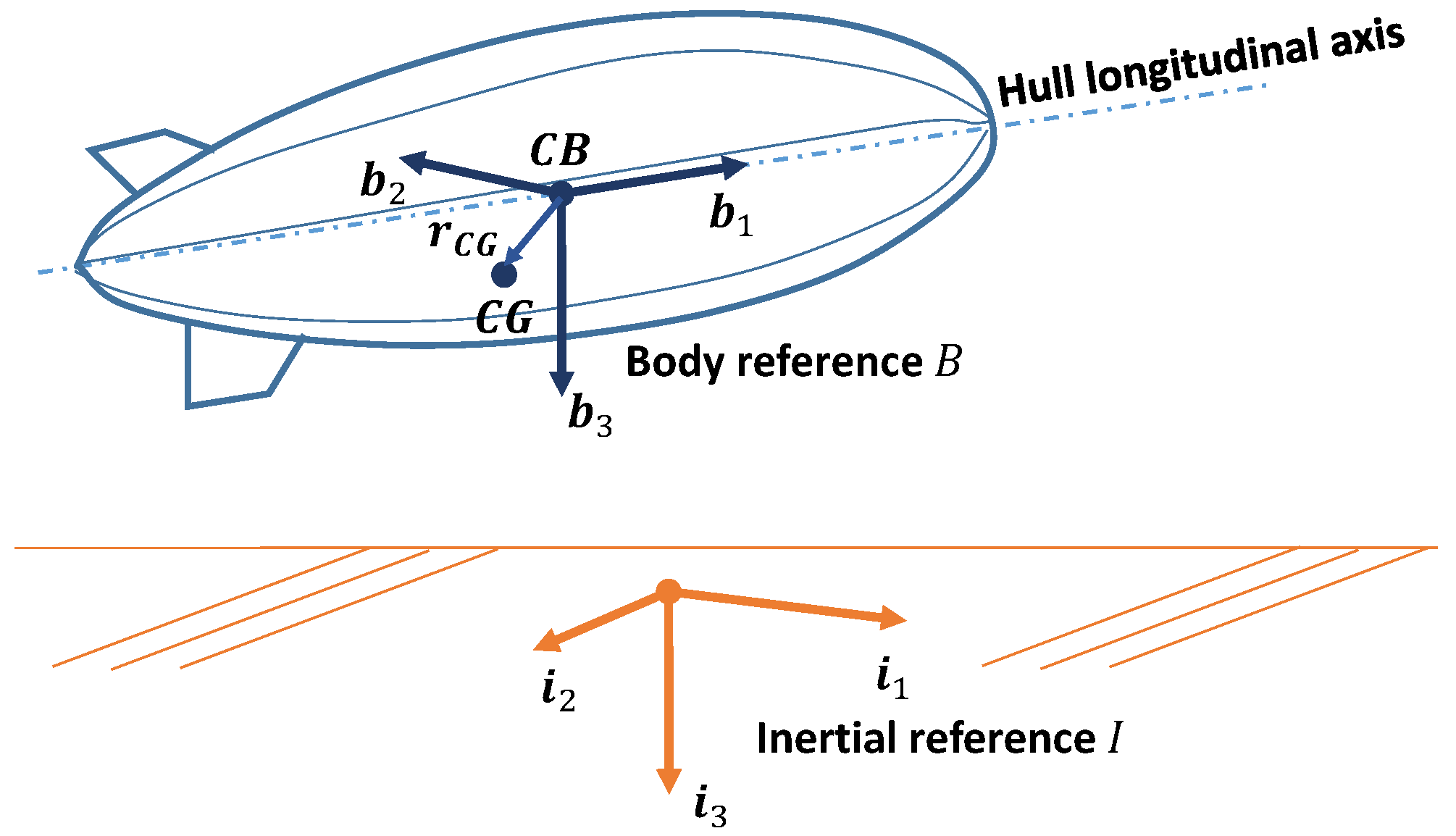
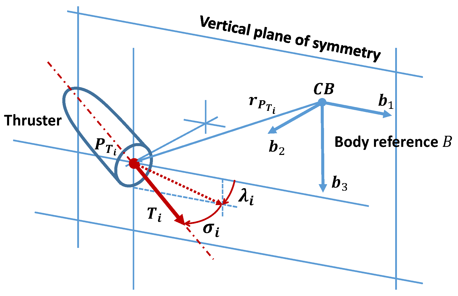
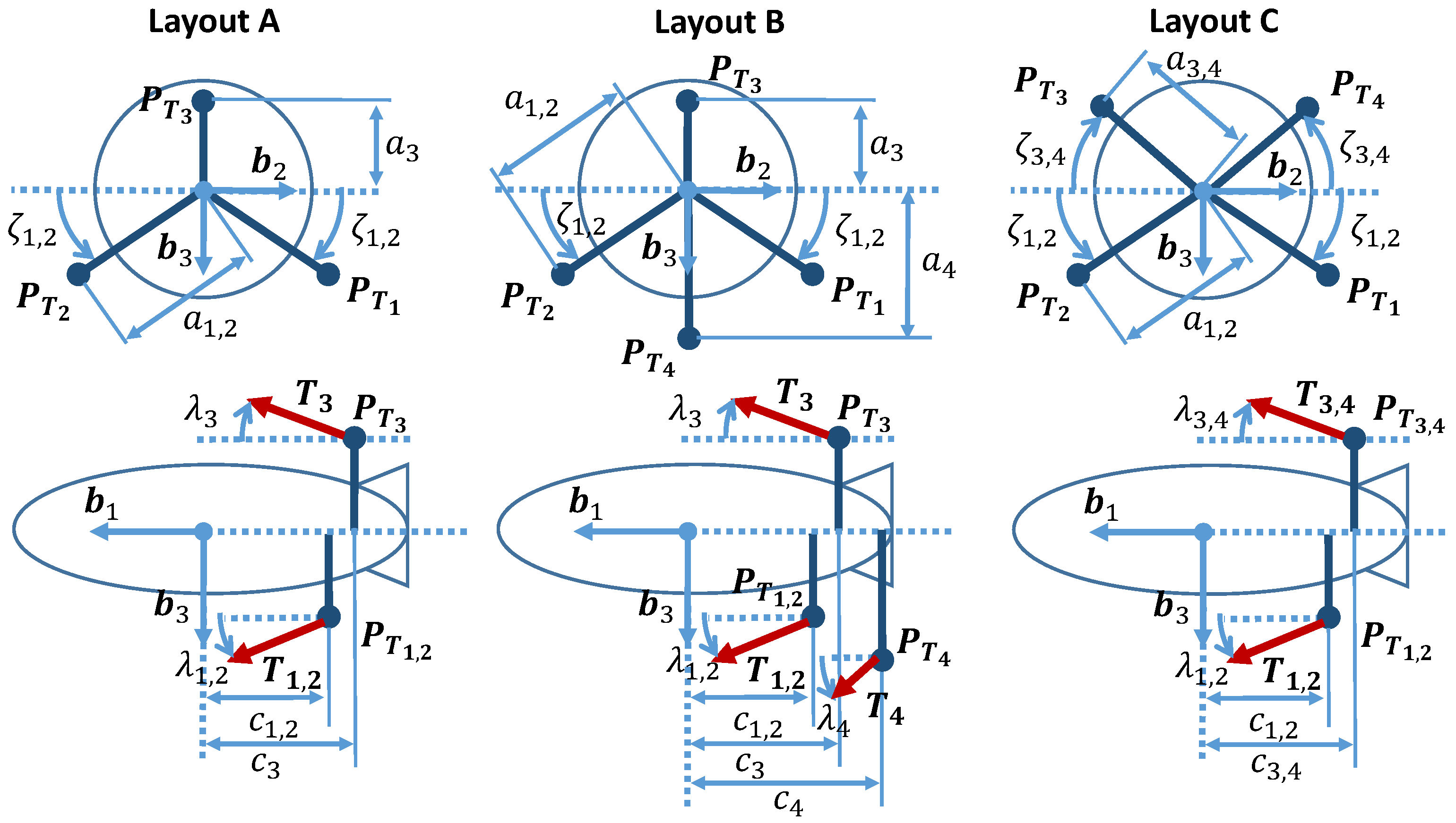
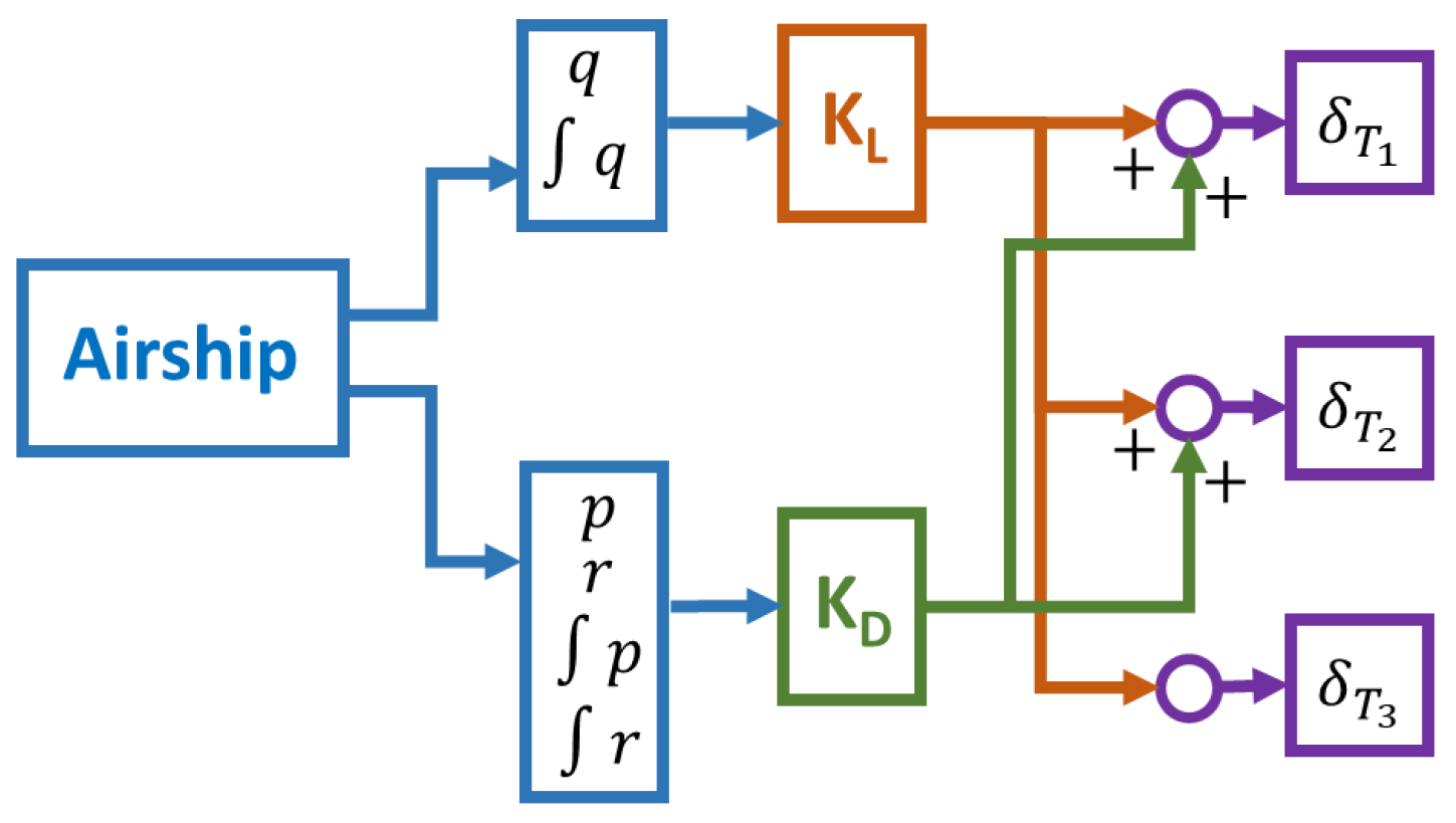
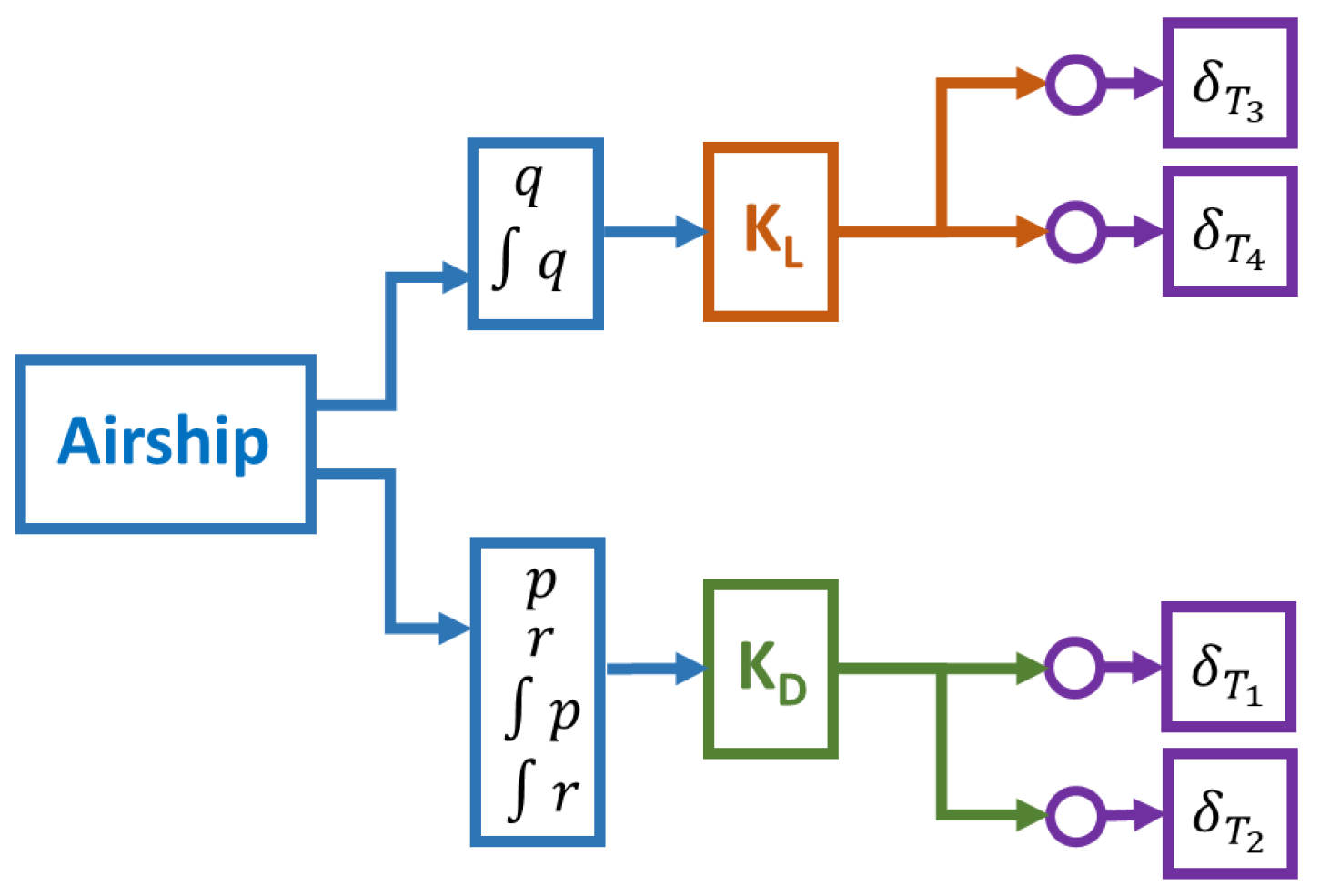
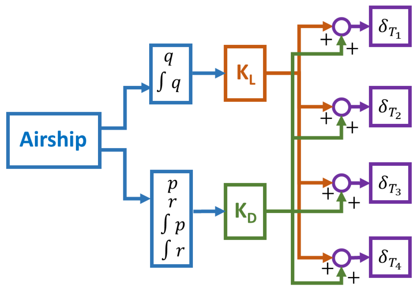
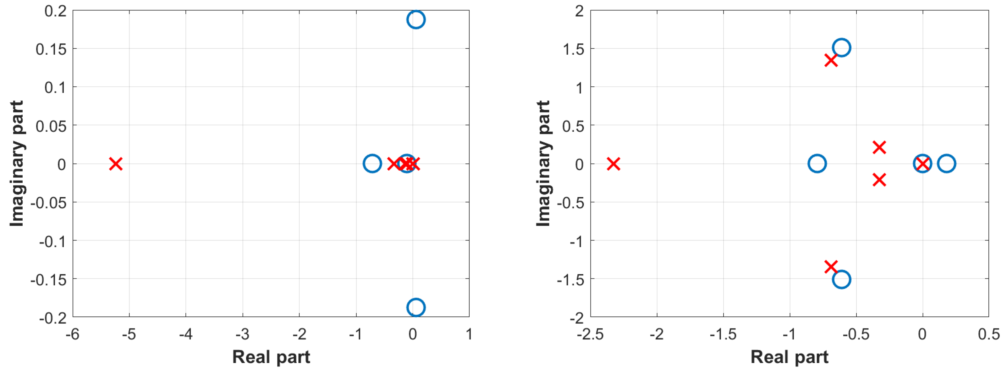
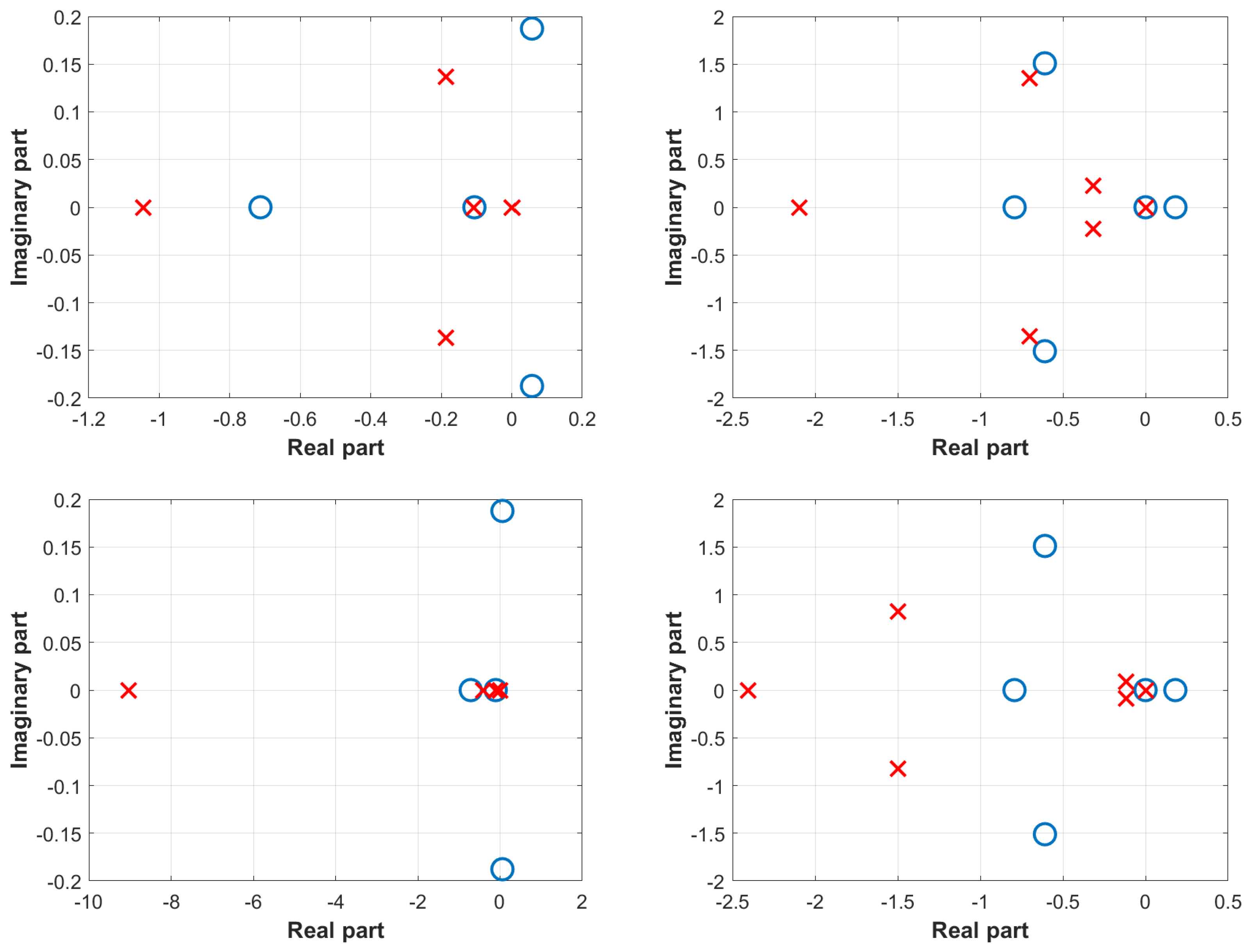
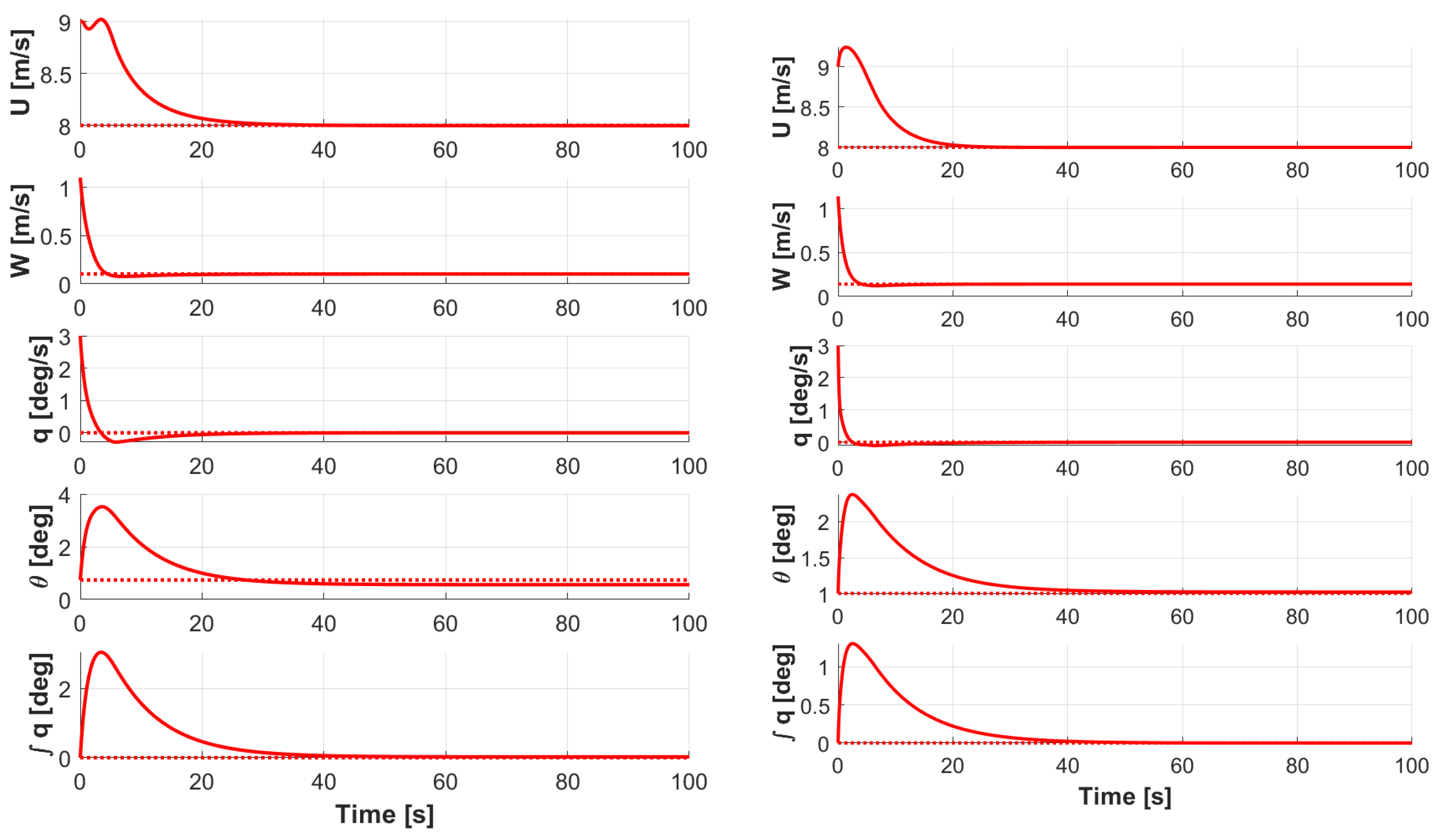
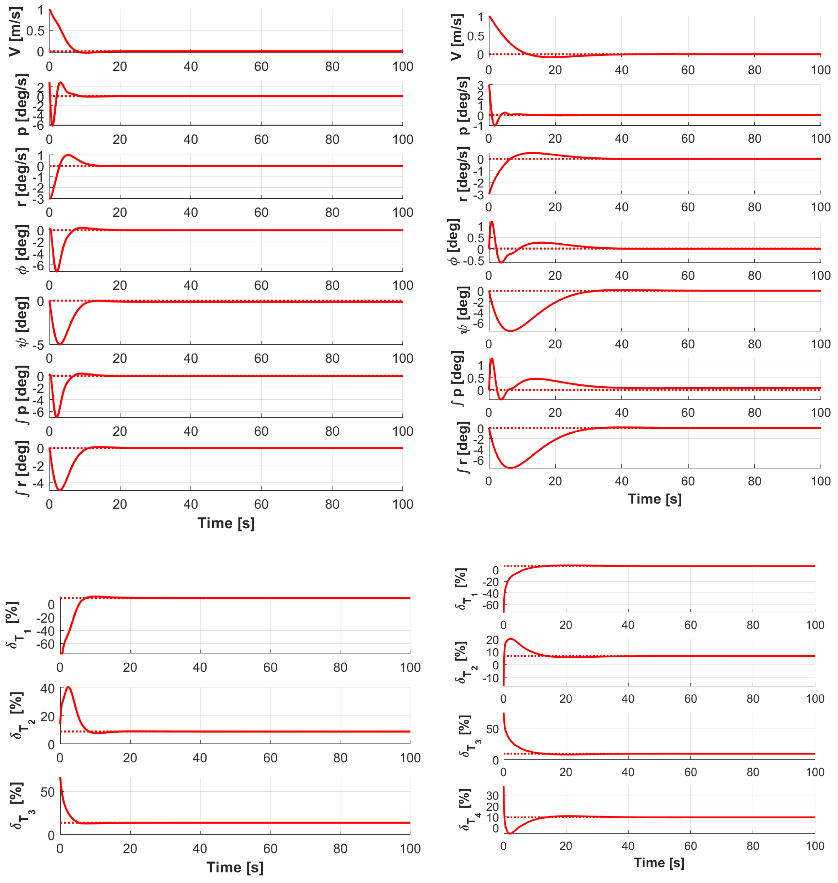
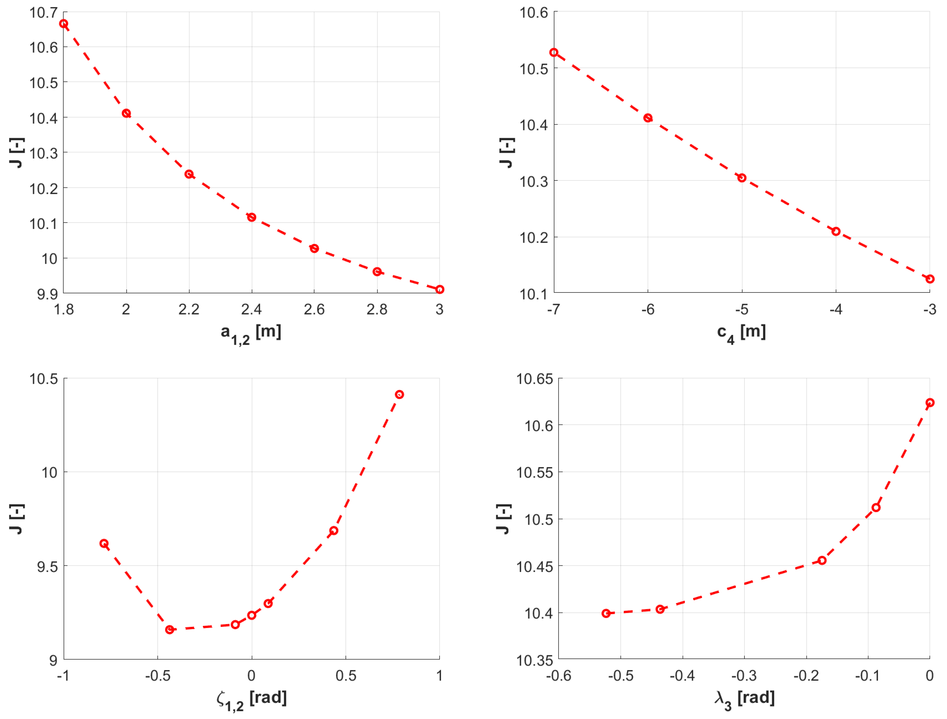
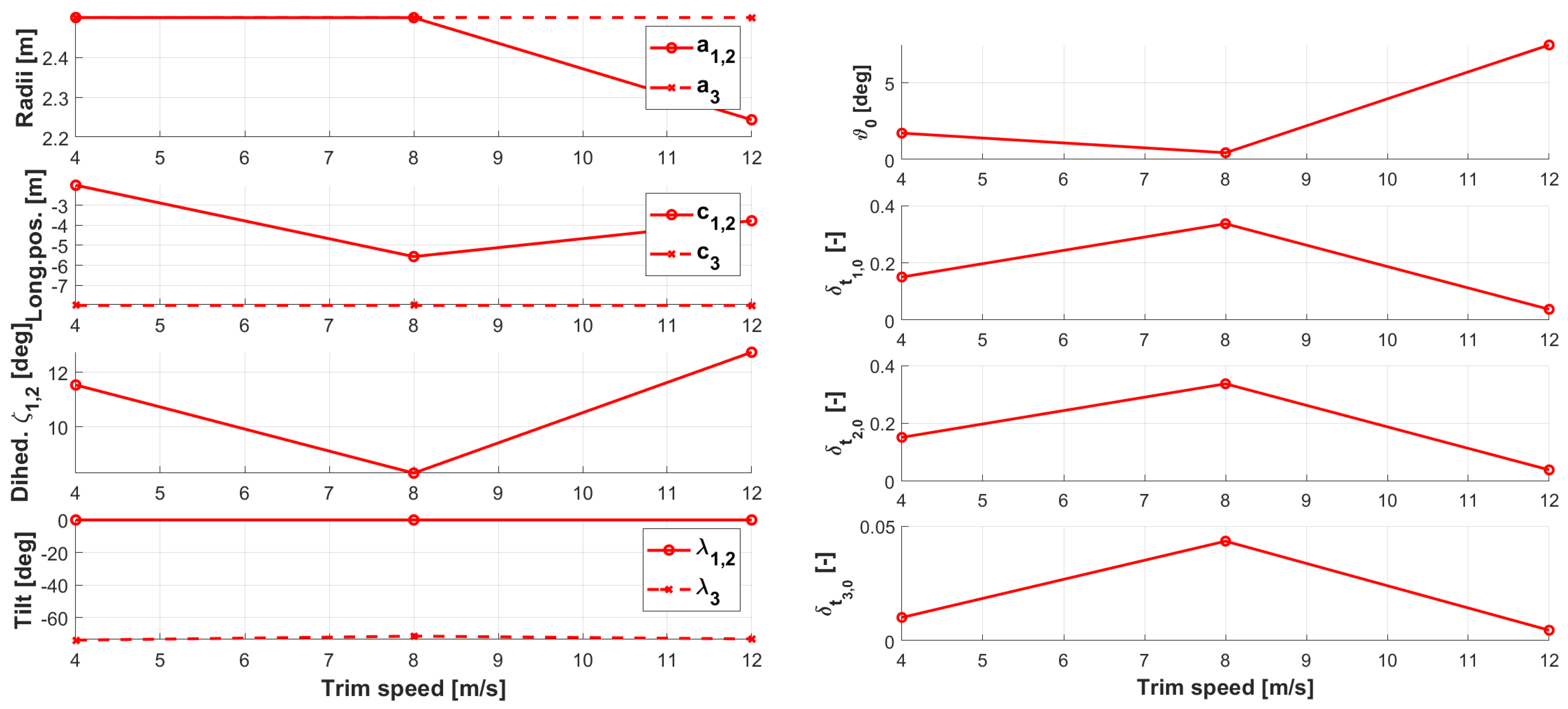
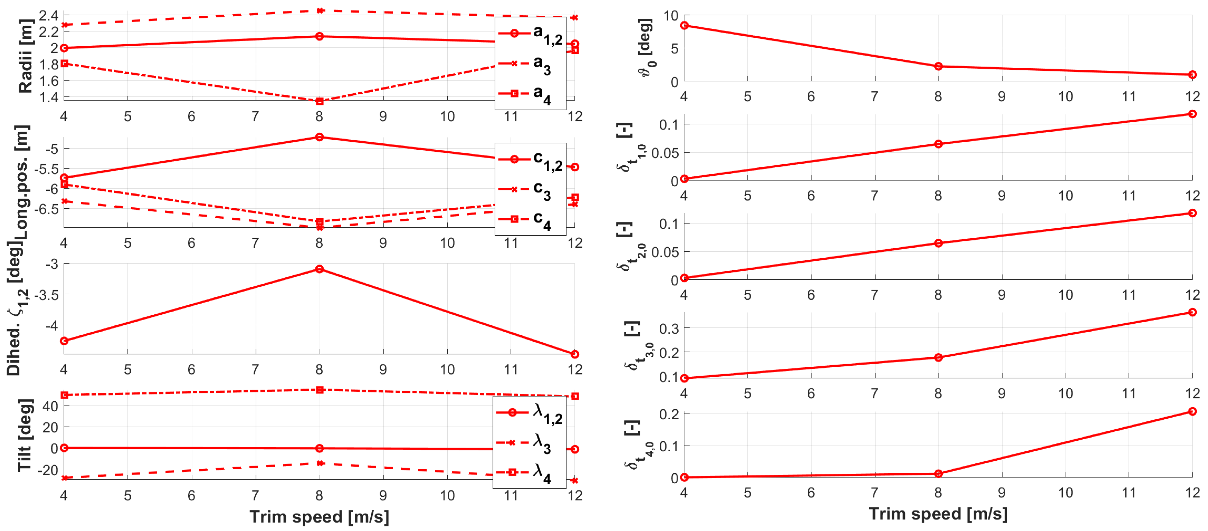
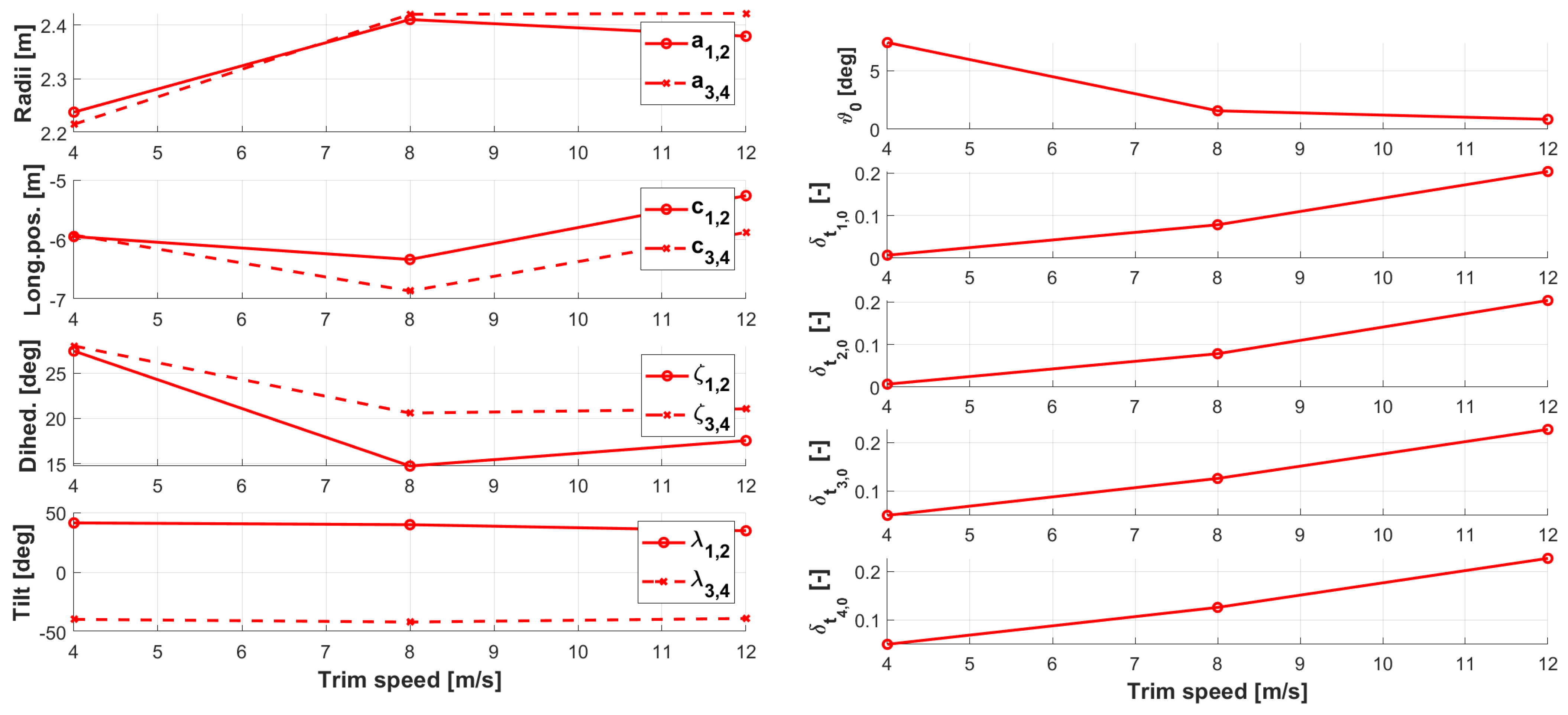
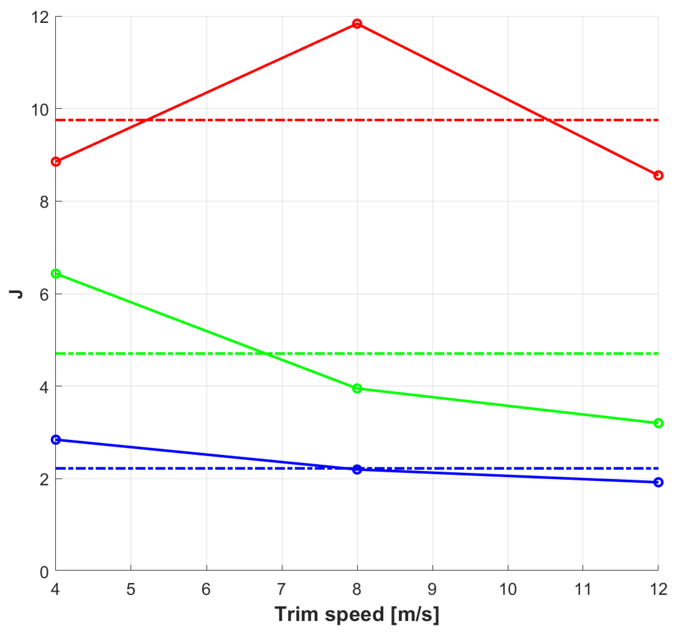
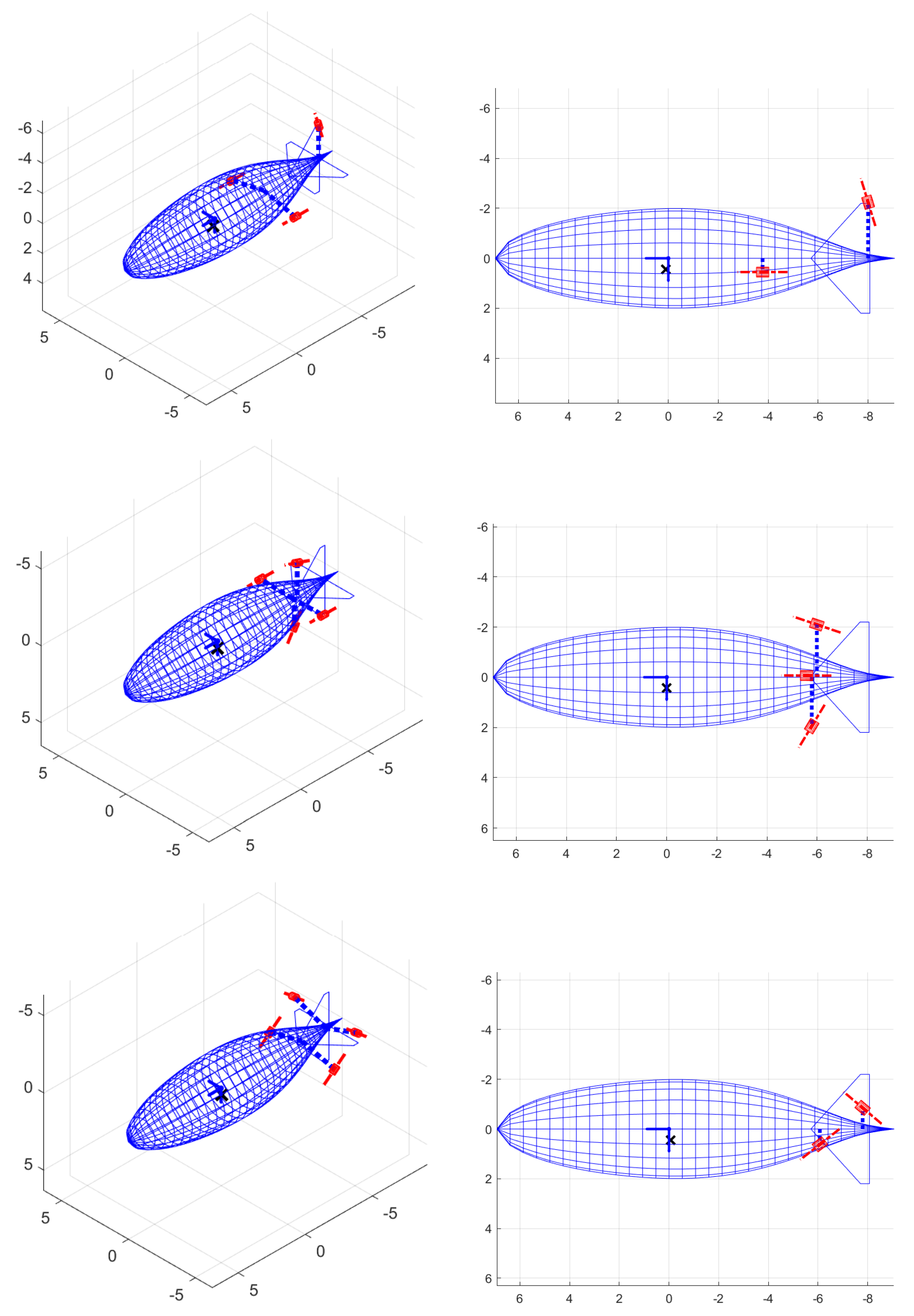
Table 1.
Sets of optimization parameters and corresponding bounds according to geometrical definitions, for the three considered thruster layouts.
Table 1.
Sets of optimization parameters and corresponding bounds according to geometrical definitions, for the three considered thruster layouts.
| Layout | (A) | (B) | (C) | |||
|---|---|---|---|---|---|---|
| ID | z | Bounds | z | Bounds | z | Bounds |
Table 2.
Basic specifications of Lotte airship [22].
Table 2.
Basic specifications of Lotte airship [22].
| Parameter | Value |
|---|---|
| Volume (m3) | 107.42 |
| Length (m) | 16.0 |
| Max. diameter (m) | 4.0 |
| Tail span (m) | 4.6 |
| Mass m (kg) | 136.8 |
| Max. airspeed (m/s) | 12 |
Table 3.
Geometry settings for all considered configurations for SAS performance study.
| Layout | (A) | (B) | (C) | |||
|---|---|---|---|---|---|---|
| ID | Param. | Value | Param. | Value | Param. | Value |
Table 4.
Optimal results from global optimizations, for the three considered layouts.
| Layout | (A) | (B) | (C) | |||
|---|---|---|---|---|---|---|
| ID | Param. | Value | Param. | Value | Param. | Value |
Publisher’s Note: MDPI stays neutral with regard to jurisdictional claims in published maps and institutional affiliations. |
© 2022 by the authors. Licensee MDPI, Basel, Switzerland. This article is an open access article distributed under the terms and conditions of the Creative Commons Attribution (CC BY) license (https://creativecommons.org/licenses/by/4.0/).
Share and Cite
MDPI and ACS Style
Riboldi, C.E.D.; Rolando, A. Layout Analysis and Optimization of Airships with Thrust-Based Stability Augmentation. Aerospace 2022, 9, 393. https://doi.org/10.3390/aerospace9070393
AMA Style
Riboldi CED, Rolando A. Layout Analysis and Optimization of Airships with Thrust-Based Stability Augmentation. Aerospace. 2022; 9(7):393. https://doi.org/10.3390/aerospace9070393
Chicago/Turabian StyleRiboldi, Carlo E. D., and Alberto Rolando. 2022. "Layout Analysis and Optimization of Airships with Thrust-Based Stability Augmentation" Aerospace 9, no. 7: 393. https://doi.org/10.3390/aerospace9070393
Note that from the first issue of 2016, this journal uses article numbers instead of page numbers. See further details here.