
On the Estimation of Vector Wind Profiles Using Aircraft-Derived Data and Gaussian Process Regression


1
School of Telecommunication Engineering, Universidad Rey Juan Carlos, Fuenlabrada, 28942 Madrid, Spain
2
Faculty of Aerospace Engineering, Delft University of Technology, 2629 HS Delft, The Netherlands
*
Author to whom correspondence should be addressed.
Aerospace 2022, 9(7), 377; https://doi.org/10.3390/aerospace9070377
Submission received: 2 June 2022
/
Revised: 1 July 2022
/
Accepted: 3 July 2022
/
Published: 13 July 2022
(This article belongs to the Special Issue Advances in Air Traffic and Airspace Control and Management)
Abstract
:This work addresses the problem of vertical wind profile online estimation at a given location. Specifically, the north and east components of the wind are continuously estimated as functions of time and altitude at two waypoints used for landing on the Adolfo Suarez Madrid-Barajas airport. A continuous nowcast of the wind profile is performed in which wind observations are derived from the aircraft states and assimilated into the model. It is well known that wind is one of the utmost contributors to uncertainties in the current and future paradigm of Air Traffic Management. Accurate wind information is key in continuous climb and descent operations, spacing, four dimensional trajectory-based operations, and aircraft performance studies, among others. In this work, wind data are obtained indirectly from the aircraft’s states broadcast by the Mode S and ADS-B aircraft surveillance systems. The Gaussian process regression is adapted to this framework and used to solve the problem. The presented method allows to construct a complete vector wind profile at any specific position that is continuous in time and altitude; namely, there is no need for grid points and time discretisation. The Gaussian process regression is a very flexible estimator which is statistically consistent under general conditions, meaning that it converges to the underground truth when more and more data are dispensed. In addition, the Gaussian process regression approach provides the whole probability distribution of any particular estimation, allowing confidence intervals to be computed naturally. In the case study presented in this paper, in which the wind is constantly estimated, the Gaussian process regression model is iteratively updated every 15 min to capture possible changes in the wind behaviour and give an estimation of the wind profile every half a minute. The method has been validated using a test dataset, achieving a reduction of 50% of the prediction uncertainty in comparison to a baseline model. Moreover, two popular wind profile estimators based on the Kalman filter are also implemented for the sake of comparison. The Kalman filter outperforms the baseline model, but it does not outperform the Gaussian process regression with errors higher by around 35%, in comparison. The obtained results show that the Gaussian process regression of aircraft-derived data reliably nowcast the wind state, which is key in Air Traffic Management.
1. Introduction
Uncertainty is an essential factor in Air Traffic Management (ATM). The ATM system is a sophisticated socio-technical structure consisting of multiple and heterogeneous components that keeps air traffic flowing [1]. The uncertainty is understood as the lack of safe and clear knowledge of something; in ATM, this can be presented in the data used, aircraft operation and decisions made by actors, equipment, and meteorology.
In ATM, the uncertainty coming from meteorology is most important [2]. It is necessary to find ways to efficiently track the present and future state of the weather in order to be taken into account in the different ATM procedures. Today, air traffic controllers and pilots mostly rely on Numerical Weather Prediction (NWP) wind reports, such as National Oceanic and Atmospheric Administration Rapid Refresh [3], which has a coarse 13-kilometre grid and is updated, at the most, once every hour. The interest in having predictions as accurate as possible leads to the incorporation of aircraft observations into NWP models, with the aim of improving said forecasts.
The most prominent cause of air traffic delay in Europe is the weather, where almost half of all regulated airport traffic delays are due to adverse weather conditions [2]. In contrast, in EEUU, 69% of delays greater than 15 min are caused by weather [4].
There are several ongoing projects with the aim of satisfying the ATM requirements through the incorporation of new emerging technologies, such as the Single European Sky ATM Research (SESAR) [5]. Wind profiles are used in continuous climb and descent operations, for instance, optimal profile descent, time of arrival control, or spacing [6,7,8]. Moreover, wind information is introduced to the Flight Management System (FMS) to perform trajectory parameters predictions, such as fuel and time. FMSs are able to store wind and temperature information at waypoints and have typically five altitude points that can contain wind information, and linearly interpolates between these altitudes and extrapolates beyond. The number of altitude levels is expected to increase as it occurs in the controlled time of arrival function used in SESAR’s initial 4D project, which uses 10 levels [9]. Since the algorithm proposed in this paper continuously estimates the wind, by supposing it can be modelled as a Gaussian stochastic process, any number of altitude levels are available.
The NWP models, which are used in ATM, have inherent flaws such as over-smoothness, absence of local variation, a coarse grid resolution, and a long update time interval, all of which render the NWP ineffective for ATM [10]. In addition, the majority of the NWP observations come from ground stations and weather balloons which are launched at particular times and places no more than four times per day. These constraints are unlikely to meet the ATM system’s actual requirements.
The necessity for precise and on-demand weather predictions leads to the usage of aircraft-derived data, in which meteorological information is derived from aircraft states [11,12]. A high grid resolution and on-demand refresh rate are two potential advantages of a prediction methodology based on aircraft-derived data. The data refresh rate is within tenths of a second [13]. As a result, aircraft-derived data has lately been used in practical ATM studies [6,8,14]. It is expected that the availability of meteorological airborne data will improve in the future. Indeed, the ongoing European System-Wide Information Management (SWIM) project has the objective to achieve a full integration of flight information to create a synchronised view of flight data by all stakeholders [15]. The SWIM project has the potential to increase the availability and consistency of meteorological data shared by airborne aircraft. Thus, the presented method may take advantage of the envisioned future of ATM, in which data are centralised and aircraft may act as a moving atmospheric sensor.
Automatic Dependent Surveillance-Broadcast (ADS-B) and Mode S aircraft data are used in this study. ADS-B is a surveillance technology that broadcasts aircraft flight states, and Mode S is an interrogation protocol. Information such as position, Mach, airspeed, ground speed, roll, and heading angle is transmitted by aircraft equipped with these technologies. The vectorial relationship between airspeed, ground speed, and the wind is used to derive wind data indirectly from the states of the aircraft. Later on in this work, these technologies as well as the wind inference process are described.
Data assimilation techniques have been proposed in the literature to take advantage of non-traditional meteorological observations, including data derived from aircraft. Most assimilation strategies, however, are focused on assimilating non-conventional meteorological data into NWP models [16,17], and hence, are prone to the drawbacks of the NWP models previously discussed. The data assimilation techniques employed in this article do not employ NWP models. The methods are based on statistical approaches and allow for the use of a huge amount of live flight data. In fact, according to Flightradar24 [18], over 10,000 planes are flying around the world at any given moment, averaging 188,901 of flights each day. This is also an advantage over the NWP models. Indeed, the assimilation of airborne data into NWP models is possible due to technologies such as the aircraft meteorological data relay [19] and the meteorological routine air report [20]; however, this information is limited since most aircraft choose not to equip these technologies and even then, the information is not always interrogated by air traffic controllers radars. In our experimental studies, less than 5% of the Mode S data emitted by aircraft were found to be of this type.
In this work, the wind profile is estimated using aircraft-derived wind observations. The north and east wind components are estimated as a function of time and altitude at a particular geographic location. More specifically, two waypoints located close to the Adolfo Suarez Madrid-Barajas (LEMD) airport, and altitudes that range from 1000 to 20,000 ft with a vertical separation of 500 ft are chosen. For this estimation, observations within a radius of 250 km are considered. The Gaussian Process Regression (GPR) methodology is adapted to our framework. Furthermore, two state-of-the-art Kalman Filters (KF) detailed in [8,21], which were used for wind-speed estimation, are also implemented and generalised to estimate both wind components. The KF-based methods and the GPR are compared. Despite some points at fixed altitude having been chosen for the wind profile, it is worth mentioning that GPR does not need a grid discretisation and can perform estimation in a continuum, unlike KF-based methods.
Surveillance-derived wind information has shown a favourable impact on the ATM framework. Aircraft wind data were utilized to recreate the wind profile using B-splines in [6], which was then used to optimally update aircraft descent trajectories in real time. In [22], wind uncertainty was represented using a statistical model that included the correlation of four different sources of uncertainty and a filter to describe the evolution of wind uncertainty over time, with the goal of determining the impact of wind forecast uncertainty on aircraft trajectory prediction. Other works studied the quality of wind field reconstruction [23] or partial reconstructing [13] using aircraft-derived data. In [8], Kalman filtering was employed to create a moving-aircraft wind-speed profile for continuous descent operations and spacing performance. In [24,25], Kalman filtering was used in a wind-field estimation to reduce measurement noise. In [14], the Kalman filtering technique was used to estimate wind in aircraft turns with a high-roll angle. Finally, in [21], GPR was introduced for wind-speed profile estimation by the authors. To the best of the authors’ knowledge, GPR models have not been used in this context.
The contribution of this paper is to provide a method to efficiently assimilate aircraft-derived wind observations in real time to generate nowcasts of the wind profile. The method is not only capable to provide an estimation but, under the Gaussian process regression approach, the whole probability distribution of any particular estimation is available. This allows, for example, to compute a confidence interval straightforwardly. In addition, a comparison with state-of-the-art KF-based methods [8,21] was carried out, showing that GPR achieves a reduction of around 35% of the estimation accuracy. Unlike previous approaches such as [6,8,21], in which only wind speed is estimated, in this paper, both north and east wind components are estimated. With regard to the nowcast of the vertical wind profile, the GPR adaptation implemented in this paper is iterative and fast, which enables data assimilation.
The paper is structured as follows: In Section 2.1, the procedure to derive the wind from ADS-B and Mode S data are described. In Section 2.2, the wind profile scenario studied in this work is detailed. In Section 2.3 and Section 2.4, the mathematical development of the KF-based methods and the GPR are described, respectively. In Section 3, the parameters set up are described, and the performance of the wind profile estimators is tested. Finally, conclusions are drawn in Section 4.
2. Methods
2.1. Deriving Wind Velocity from ADS-B and Mode S Data
In this Section, the used aircraft-derived data and the procedure through which wind velocity information is derived from said data are discussed. In this paper, the term wind velocity denotes the vector quantity that indicates the rate at which air particles in the atmosphere change their position. The wind vector used in this paper is horizontal, that is, it measures the rate of change in the north and east direction. The term wind speed denotes the scalar quantity that corresponds to the module of the wind velocity vector. Within this paper, the wind velocity vector will often be characterised by its wind speed and direction. If the context is clear, only wind may be used to refer to the wind velocity (vector) to favour the reading.
2.1.1. ADS-B and Mode S
ADS-B is a surveillance technology that enables the automatic broadcast of aircraft flight states. ADS-B relies primarily on the Global Navigation Systems to obtain the flight states of position and ground speed, which are transmitted periodically at a rate of every 0.5 s, approximately.
The most common implementation of ADS-B is through the Mode S extended squitter. Mode S is a selective interrogation protocol employed by air traffic controllers to obtain additional flight states other than the position and altitude. Within Mode S Enhanced Surveillance (EHS) communication protocol, a set of parameters related to aircraft airspeed are interrogated by surveillance radar and transmitted by aircraft.
Mode S signals, including ADS-B signals, can be openly received by researchers around the world. The inference and decoding of these signals can also be achieved using the open-source tool pyModeS [26], which is employed in this work. Ground speed, track angle, true airspeed, and heading angle are used to generate the wind observations.
The ground speed of an aircraft is its horizontal velocity relative to the Earth’s surface. The True Airspeed (TAS) of an aircraft is its velocity relative to the atmosphere. Both are vector quantities that, in aviation terminology, contain the term speed, which in physics, denotes a scalar quantity. The indicated airspeed is the airspeed displayed on the flight-deck instruments and coincides with TAS when there is no wind and a pressure of 1013.2 mb.
The heading angle of an aircraft describes the direction in which the aircraft is pointed. Note that the heading angle may not necessarily be the direction that the vehicle is actually following, which is known as its course or track. The difference between the heading and track is known as the drift. This is due to the motion of the air around the aircraft, i.e., the wind, which can be determined by the wind triangle.
2.1.2. Wind Velocity Derivation
In order to infer the wind, the true airspeed needs to be calculated first, based on the Mach number and indicated airspeed that is transmitted by the aircraft in the Mode S communication system. This is carried out using aeronautical airspeed conversions based on the International Standard Atmosphere (ISA) model, which is an atmospheric model that provides atmosphere changes in pressure, temperature, density, and viscosity over a wide range of altitudes.
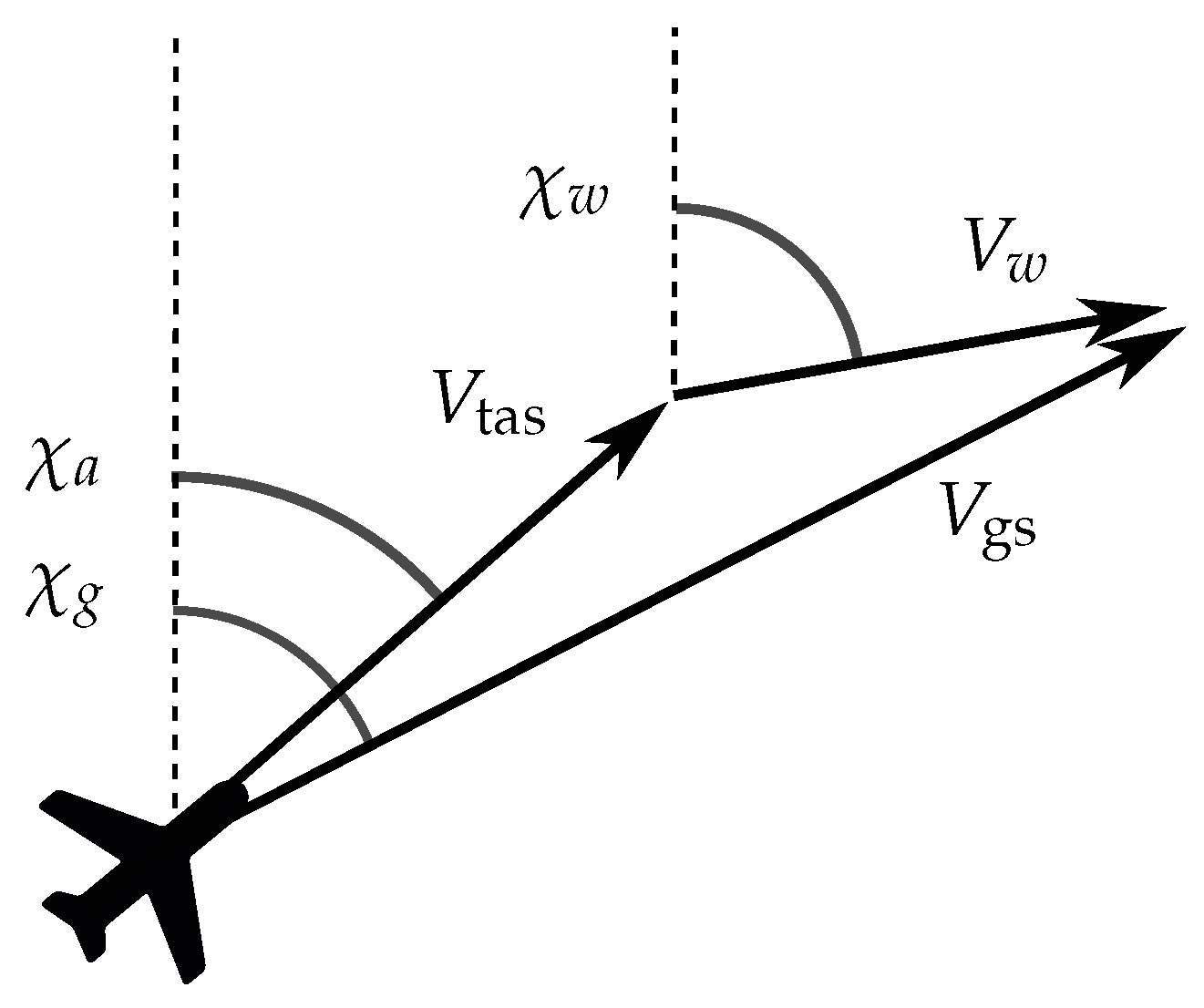
Once the true airspeed, ground speed, heading and track angles are known, the wind vector can be calculated as the difference between the ground speed vector and the true airspeed vector. In Figure 1, the relationship among these vectors is illustrated. Here, , , and represent the track, heading, and wind direction angles, while , , and represent the ground speed, true airspeed, and wind-speed vectors, respectively.
The wind velocity observations obtained from different aircraft are used for wind profile estimations.
2.2. Vector Wind Profile
The wind profile is a vertical representation of the horizontal mean wind speed. The log wind profile and the power law wind profile are common models for describing the wind profile the under genera conditions [27,28]. In this paper, the speed and direction of the wind are estimated, both of which are crucial in the ATM framework. Thus, a profile including the direction of the wind is referred to as a Vector Wind Profile (VWP) and consists of an estimation of the wind velocity vector along with the altitude domain at specific locations [29,30].
Particularly, in this work, the estimation of the VWP is carried out at two fixed waypoints located at the TMA of the LEMD airport. More specifically, the RILKO IAF and FAF waypoints are considered, which are located at 3.3 km and 1.2 km of altitude, respectively, close to the LEMD airport. These vertical profiles range from 2000 ft (0.61 km) to 20,000 ft (6.1 km), over the sea level. The dataset used is an all-purpose structured EUROCONTROL surveillance information exchange (ASTERIX) dataset, which was provided by the Spanish National Air Navigation Service Provider (ENAIRE). The ADS-B and Mode S information has been extracted from the ASTERIX dataset which, in our case, contains information for 21 September 2019, which is a day with high wind speed. In particular, the mean wind speed, below 6.1 km of altitude, is 31.5 m/s, one of the windiest days of 2019.
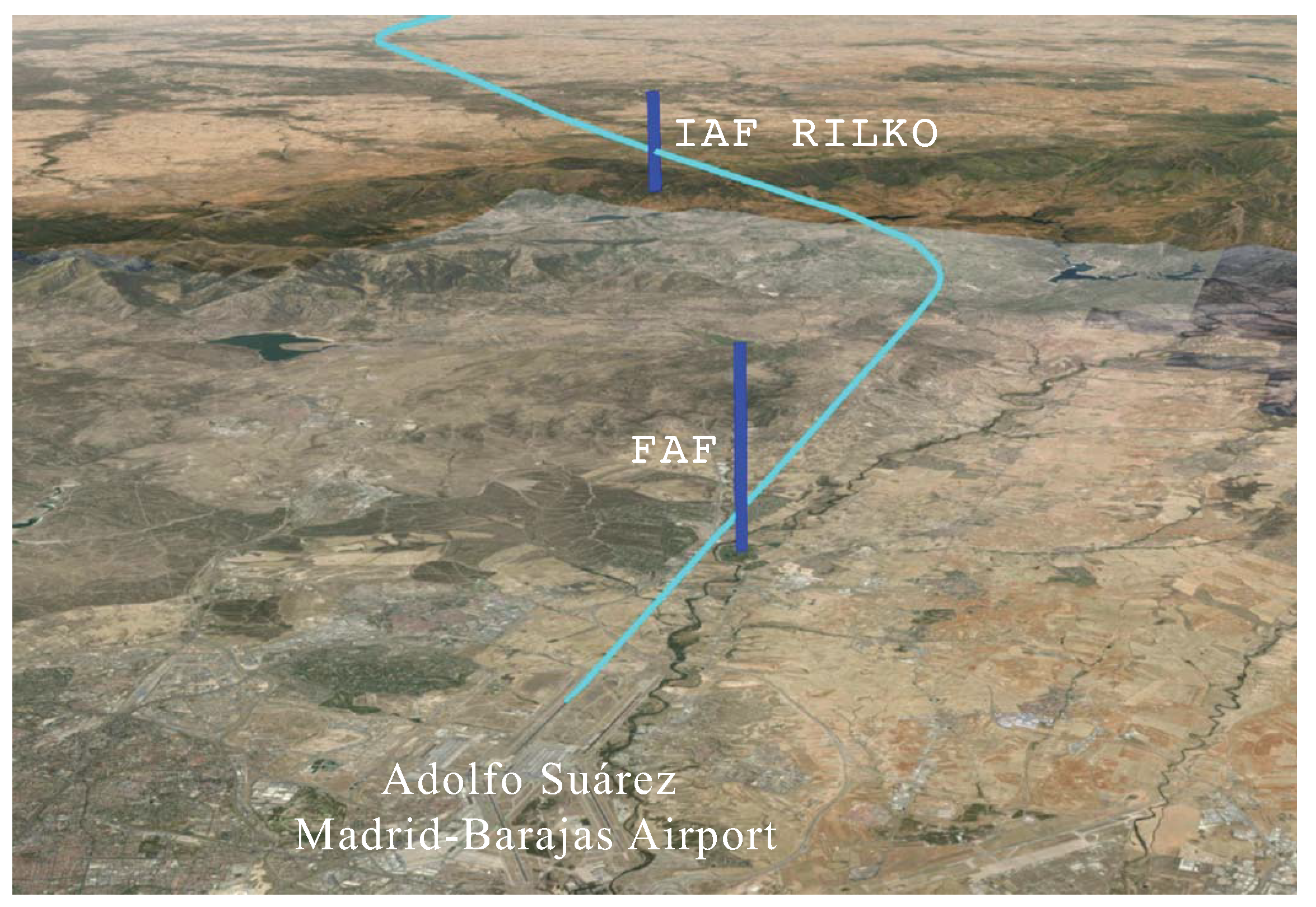
A landing flight trajectory, the two waypoints, and the position of the VWPs are illustrated in Figure 2. Due to operational constraints, all the flights heading to the LEMD airport must pass through the FAF waypoint before landing.
2.3. The Kalman Filter-Based Models
The Kalman Filter (KF) is a popular technique for sequential interpolation [31] and is widely used in the data assimilation discipline. A continuous-time version of the filter was given by Bucy [32]. The Kalman filter can be introduced in several ways, for example, from a Bayesian filtering perspective view. See [33] for a comprehensive review of the literature.
A variant of the Kalman filter was used in [8] for constructing a wind-speed profile estimation and more recently in [21] for a waypoint wind-speed profile estimation by the current authors. In this paper, we propose an adaptation of the Kalman filter methodology to construct a wind profile estimator, not just for the wind speed, but for the wind vector itself.
Typically, the KF has two stochastic equations:
where the model errors and are assumed to be unbiased and uncorrelated. The errors covariance matrices are denoted as
The state Equation (1a) models the dynamics of the system, which is considered an unobserved or hidden state. It describes the time evolution of the system. On the other hand, the measurement Equation (1b) describes the relationship between the observation and the true states of the variables.
This ansatz, although it may look simple, is very general and allows for modelling any system in which the variables of interest can be embedded in a vector. For example, could represent the position and velocity of an object over time or be the parameters of an autoregressive process . In our case, will contain the wind vectors at each discretised altitude. A more complex system, where the linear operators and are substituted by general operators, can also be considered with specific adaptations of the Kalman filter, such as the extended Kalman filter or the Ensemble Kalman Filter (EnKF). For example, this is often the case for satellite, Lidar, and radar observations where the radiance measurements and the state variable are related in a strongly non-linear way. For other problems, such as assimilation of meteorological data in NWP models, the classical Kalman filter may be expensive and hard to afford. For a high dimensional system, one has to manipulate (covariance) matrices which require at least scalars to be stored, being n the size of the vector . This issue may be overtaken using the EnKF filter which uses the sample covariance instead and can make the computations in the ensemble space, usually of a smaller dimension. For more information about this topic, see [34,35,36]. In our case, there is no need to use these adaptations since and are linear and the wind profile is one dimensional, as described in Section 2.3.1 and Section 2.3.2.
The KF is an iterative algorithm, at each time step , the algorithm is as follows:
- If , the algorithm is initialized. An initial state vector is given as , where the superscript f indicates forecast. An error covariance matrix of this estimation, , is also given as an input.
- If :
- (a)
- Analysis
- The Kalman gain matrix is computed with the formula:. This matrix is based in the uncertainties on the current state and the new measurements.
- The state vector is updated using the new observations and :, where the superscript a stands for analysis.
- The covariance matrix of the analysis estimation is computed as:.
- (b)
- Forecast
- The forecast of states for the next time step is calculated as:.
- The error covariance matrix of this estimation is calculated as:.
In order to estimate the wind velocity, two variants are considered which we name Adapted Kalman Filter (AKF) and Smooth Adapted Kalman Filter (SAKF).
2.3.1. Adapted Kalman Filter
The AKF is a generalization of the Airborne Wind Estimation Algorithm (AWEA) [8,21]. AWEA aimed to estimate the wind speed at each discretised altitude (wind profile). Now, what is modelled, are the wind components, , at each discretised altitude. Since there are two components, two-state equations are considered, one for each wind component:
We propose to embed both vectors in a unique state vector and adapt the matrices and to be consistent with the new state vector. Concretely,
As in AWEA, the AKF method does not consider wind dynamics; therefore, is reduced to the identity matrix where n is the number of altitude levels. The H matrix is computed such that the observations are linearly interpolated in the altitude grid. Let m be the number of observations available at time step . Now, let the i-th observation be—for example, at 1700 ft—and consider a discretisation at every 500 ft, starting from 1000 ft. The closest altitude levels are 1500 ft and 2000 ft. Then,
The i-th row in the matrix H corresponds to the i-th observation for the u component and the -th to the v component. The matrix H is diagonal by boxes:
With this construction, observations are only related to those elements of the state vector that are at a similar altitude.
The matrix models the variances of the measurement error, and in AKF, it is cleverly modified to also take into account the uncertainty of observations coming from a distance. The further away an observation is, with respect to the position of the waypoint, the less trustworthy it becomes; this will be considered for the estimation of the wind. If m observations are available at time interval , the matrix becomes
where is the instrumental measurement error, is the great circle distance from the observation to the waypoint in NM, and is a scaling parameter. In this way, the uncertainty of the observation is modelled as a function of the distance. For example, if the observation is at 215 NM away and is chosen to be one, the error becomes , which is twice the typical instrumental error .
2.3.2. The Smooth Adapted Kalman Filter
The SAKF method is related to the AKF. Since wind is a continuous variable, the objective is to construct a smoother wind estimator. As is shown in Section 3.2, the VWP resulting from AKF are usually saw-shaped, generating peaks at the discretised altitude levels. To achieve a smooth estimation, the matrix is modified and is no longer a simple identity matrix. With this aim, weights are assigned to the values of the state vector , making each wind component depend on the neighbourhood points values. Thus, the following matrix is proposed:
The weights satisfy , . In this way, an updated estimation at altitude j is built as the combination of , the estimation at that point, and , the estimation at the neighbourhood points. Notice that both KF filters, AKF and SAKF, take into account the distance of the observations to the waypoints when estimating the wind profile. For instance, an observation located 100 km away from a waypoint is less trusted than an observation located 50 km away.
2.4. Gaussian Process Regression
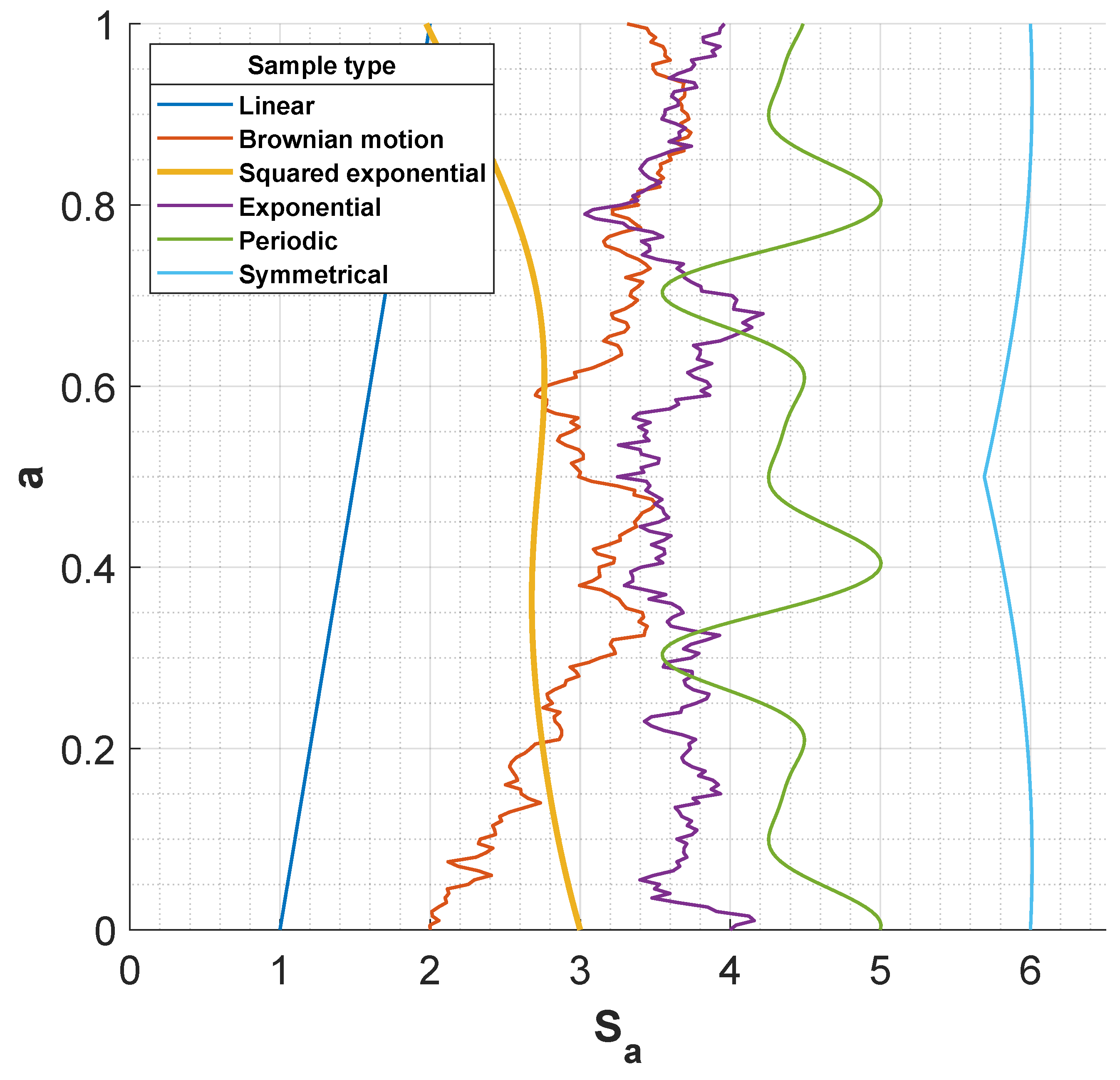
GPR is a mathematical model that relies on the idea of a Gaussian Process (GP). A GP is a stochastic process (I is the index set), such that any sample of the process is jointly Gaussian-distributed for all k, and all choices of . GP index set can be discrete or continuous. A GP sample can have a wide variety of shapes, leading to properties such as linearity, symmetry, periodicity, continuity, or smoothness. A very useful property of normal variables that GP inherits is that the process is completely determined by the mean and covariance functions. The mean function may be used to model the deterministic behaviour of the process (such as linear trends), whereas the covariance function models the correlation structure of the process and is decisive in the modelling step. In Figure 3, different GP samples are depicted as wind profiles. They are generated using distinct covariance functions, illustrating the different properties described above. GPR uses the idea of GP to fit the observed data, using probability distributions in their formulation. For this reason, GPR is an interesting tool that has applications in a wide variety of disciplines such as geostatistics or machine learning [37], where it has become increasingly popular.
A GPR models predicts the value of a scalar variable y given some predictor variables . The GPR model can be introduced as a generalisation of the classical linear regression model,
where and usually are parameters. The GPR model introduces a GP in the equation and rewrites the linear term , resulting in,
where,
- is a Gaussian process. Any sample, , is jointly Gaussian-distributed with zero-mean and some covariance function .
- h is a basis function that projects the input into a p-dimensional space and allows the trend to be, in general, non-linear.
Under these assumptions it can be seen that the predictive distribution for the variable y at a point given a training dataset (X, Y) is also Gaussian-distributed [37]. This property makes GPR a potent tool, since, in addition to the estimated value, the probability distribution of the possible values is also given. This allows, for example, to provide a confidence interval for the estimations. A VWP confidence interval, based on this predictive distribution, is going to be illustrated in Section 3.2. Interesting work connecting the GPR and related methods of machine learning—specifically the connection between GPR, Kalman filtering, and smoothing—can be found in [38].
Adaptation of GPR to Wind Velocity Output
In our case study, the objective is to predict the -components, making our problem to be multi-output. To extend the single output GPR model to multiple outputs, the adaptation that has been considered in this paper is to use an output , and then restore the wind components by computing . This adaptation has two main motivations: (1) estimating wind speed with GPR has been proven to be effective in our previous study [21], (2) separating the estimation of two physically different magnitudes (wind speed and direction) may help GPR to identify the relation between input and output and benefit the training of the GPR model. A detailed discussion on multiple-output GPR, which is an active field of research, can be found in [39,40].
3. Results
3.1. Model Set Up
In this Section, the model layouts for the KF-based methods and GPR model are presented. The initial parameters are selected and, for the GPR, a smooth parametric covariance function is chosen. In addition, a baseline model, which will act as a lower performance threshold, is introduced.
3.1.1. Kalman Filters
The chosen instrumental error is m/s according to the typical wind measurement error of this type of data described in [8]. In the KF-based methods, the initial wind-speed profile has been estimated based on a standard logarithmic wind profile according to the power law described in [28]. The initial direction of the wind is chosen by computing the mean for each wind component and then computing the angle of the resultant vector. The initial covariance matrices are:
where I stands for the identity matrix. The chosen elements of the diagonal matrix , corresponding to the forecast errors, are large enough to give uncertainty to the initial estimation. In this way, the filter will quickly adapt to new incoming data. In the observation uncertainty matrix R, the scaling parameter is set to 2. For the SAKF model, and have been set to 0.8 and 0.2, respectively.
3.1.2. GPR
For the GPR, the instrumental noise is also assumed to be 3 m/s. A parametric kernel function ) is chosen to define the covariance structure. The classical kernels used in the literature are parametric, and most of them stationary. A parametric kernel is a specific covariance function, which is defined in terms of one or several parameters. Typically, the kernel function models the covariance structure, while the parameters are chosen so that they can be adapted to the problem, such as modelling, for instance, the length scales of the input or the output standard deviation. Samples of GP realisations generated by the most common kernels are depicted in Figure 3. The squared exponential kernel, which is one of the most frequently used covariance functions [37], is chosen and adapted to this study. More specifically, the following parametric kernel function is chosen to define the covariance structure: )
where
with
being the hyperparameter vector. This kernel has some nice properties; it is universal [41,42], produces smooth samples with infinite derivatives, and the number of hyperparameters defining the kernel is interpretable and short. The kernel is defined such that the correlation between two spatio-temporal points decreases fast as a function of the Euclidean distance, where each input is scaled by a factor . This allows variables to have different length scales (anisotropic) as is the case in this work, where the inputs are time and space variables. The scaling factors can be interpreted as how far two input points should be in order to be considered practically uncorrelated. Finally, , also known as signal standard deviation, is a factor that allows adapting the auto-covariance function to the output scale.
The corresponding hyperparameters and the coefficients of the basis function, which in this work has been considered to be linear, have to be estimated through data. For a fast and accurate estimation, the subset of data points (SD) method [37] (Section 8.2) and the block coordinate descent (BCD) approximation are used [43]. The SD and BCD methods allow GPR to be calibrated in less than 5 min, allowing for data assimilation, reducing time complexity, and avoiding memory problems.
3.1.3. Baseline Vector Wind Profile
In addition to the KF-based filters and GPR, a baseline estimator is also included, which acts as a lower performance threshold. The method is intuitive; it estimates the wind by computing the mean of the wind observation per each altitude level. The filter is initiated with the same estimation as for KF methods, and if there are no data at the corresponding altitude level at a given time step, the filter remains unchanged. Notice that the baseline model has no parameters.
3.2. Performance Evaluation
The data assimilation techniques are tested using a 2 h and 5 min dataset from 21 September 2019, with an average wind of 60.6 m/s for the whole dataset, and 31.5 m/s for observations below 6.1 km (20,000 ft). The VWP estimation and validation are carried out as follows:
- 1.
- The AKF, SAKF, and baseline estimators initiate at 13:45 UTC, 15 min before validation. This time interval acts as a burn-in period.
- 2.
- The GPR model is initially trained using a previous 1 h dataset selected from 12:55 to 13:55 UTC. All landing data passing through the considered waypoints are excluded from the train dataset, and are only used for validation.
- 3.
- The validation phase starts at 14:00 UTC. The vector wind profiles are compared with the testing data coming from the landing aircraft when passing through the waypoints, namely RILKO IAF and FAF. Every 15 min, a new GPR model is trained to detect potential trend changes in the wind behaviour. Validation finishes at 15:00.
- 4.
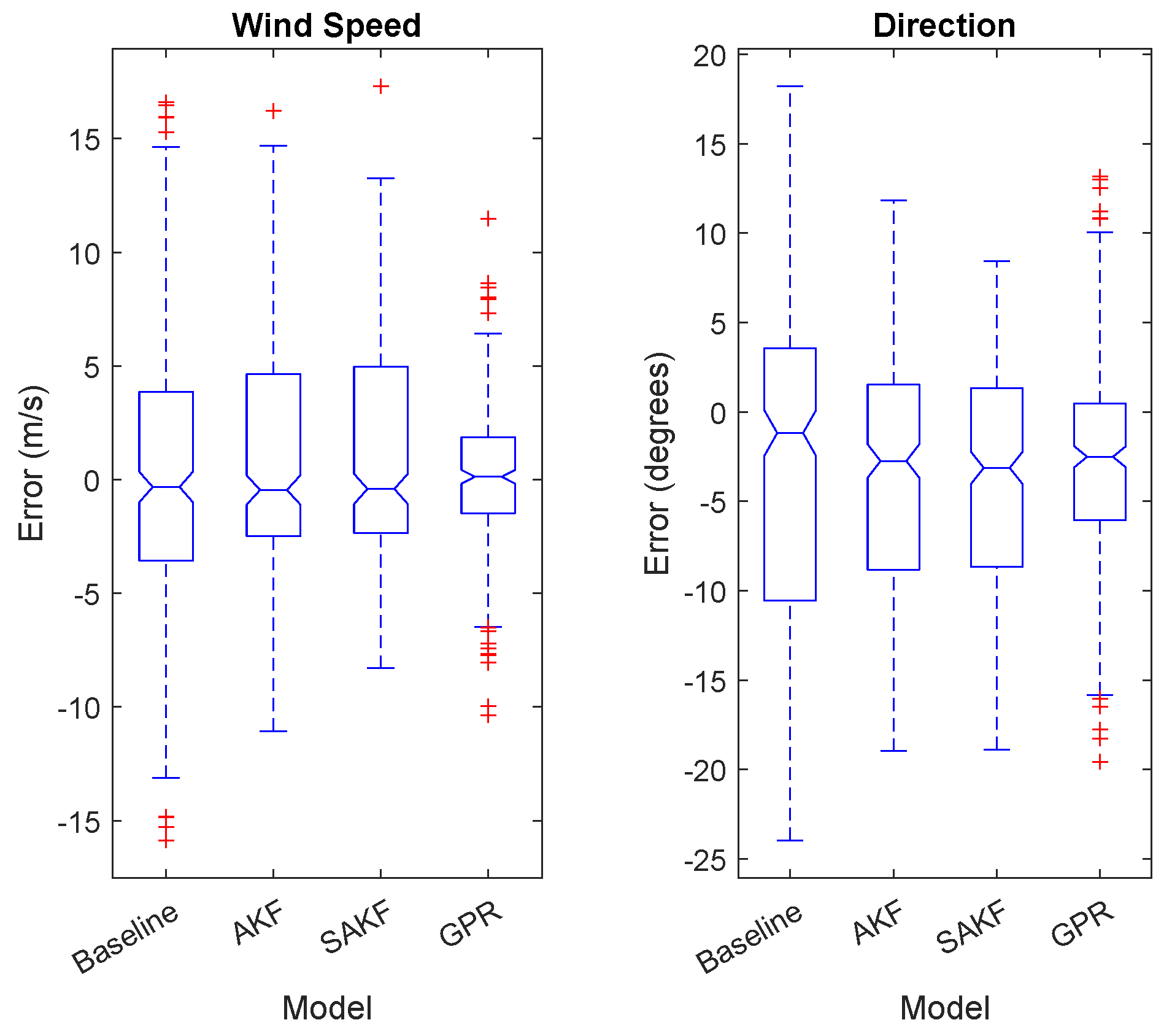
- Different performance measures are considered in order to assess the VWP estimations. The root mean square error (RMSE) and the mean absolute error (MAE) of the wind components and the wind speed are computed. In addition, boxplots of wind speed and direction errors are also obtained.
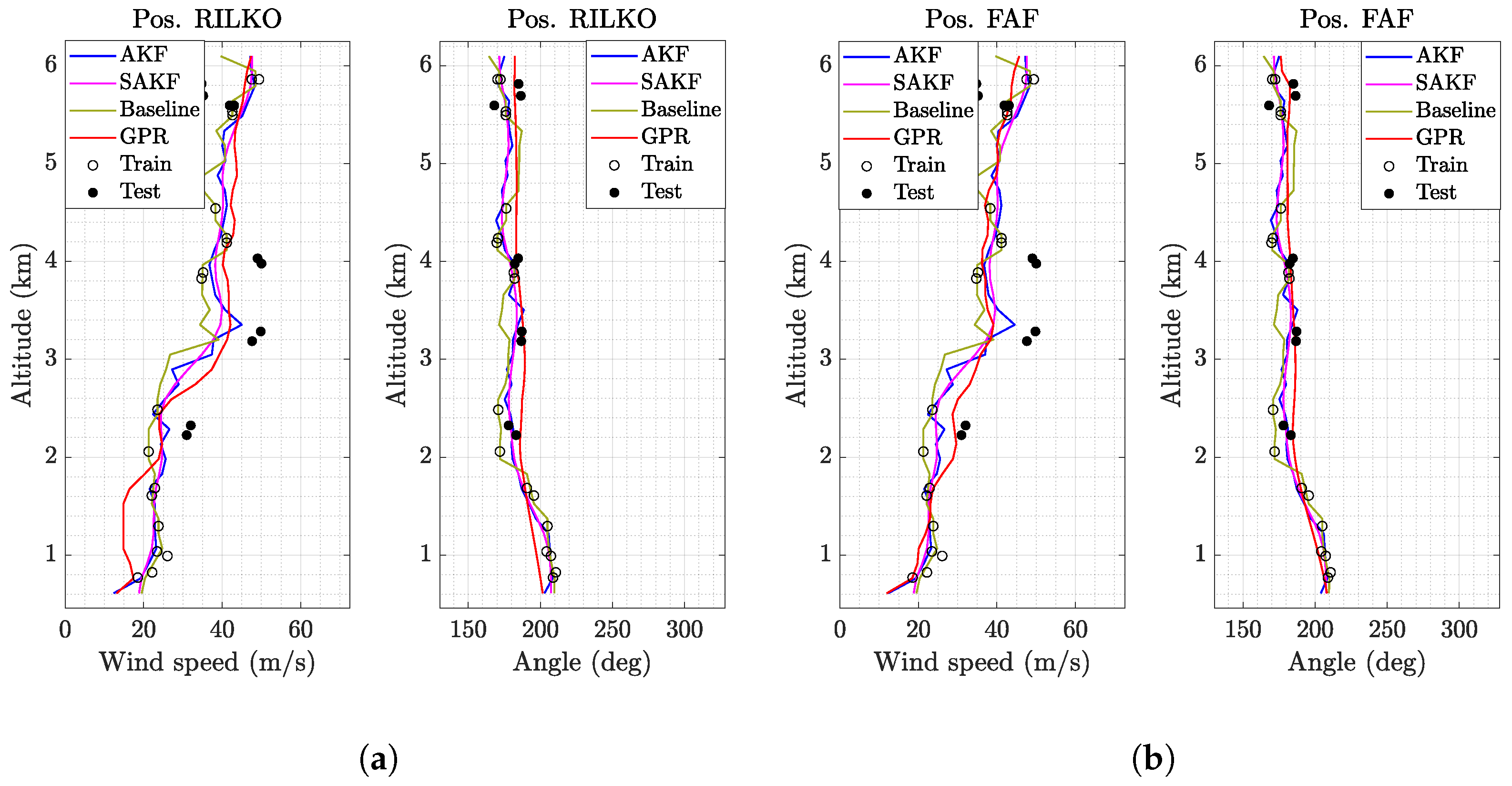
Figure 4 shows the vector wind profiles at RILKO IAF and FAF waypoints obtained using the different techniques, together with the training and testing data available at the time instant of 14:10 UTC. For an easier interpretation of the wind state, the wind speed and direction are represented instead of -components. It can be seen in Figure 4 that the estimation provided by the AKF shows a saw-shaped profile, whereas the SAKF achieves a smoother estimation while keeping the trend. GPR estimation is also smooth and shows significant differences with respect to the KF-based methods. Furthermore, the differences between the two wind profiles estimated by the GPR at RILKO IAF and FAF waypoints are noticeable, whereas these differences are not that apparent when the wind profiles are estimated using the KF-based approaches. Finally, it can be observed that the GPR and KF estimations at RILKO IAF waypoint differ at around 1.2 km of altitude, whereas they are more similar at the FAF waypoint. Actually, this is because the KF-based methods are more dependent on the availability of data close to waypoints, since for FAF, several aircraft are flying close on a nearby track which do not fly close to the RILKO IAF waypoint.
The obtained performance errors are shown in Table 1. It can be seen that all the assimilation techniques achieve a better VWP estimation in comparison to the baseline model, in which the estimations are computed by simply averaging. For the GPR method, the improvement is clear. In general, the estimation errors of the GPR halve the baseline model estimation errors, and always improve the estimation errors of the KF-based methods. Moreover, Figure 5 shows the boxplots of the wind speed and direction errors obtained for each method. It can be observed that the estimation errors of the GPR are less biased, more symmetric, and show a lower spread for both magnitudes.
Despite showing smoother VWP estimations, the SAKF does not outperform the AKF. Although smoothness is a desirable property, the ability to produce unbiased estimations and track the wind behaviour at each altitude are also important. Notice that the GPR shows the ability to combine both properties.
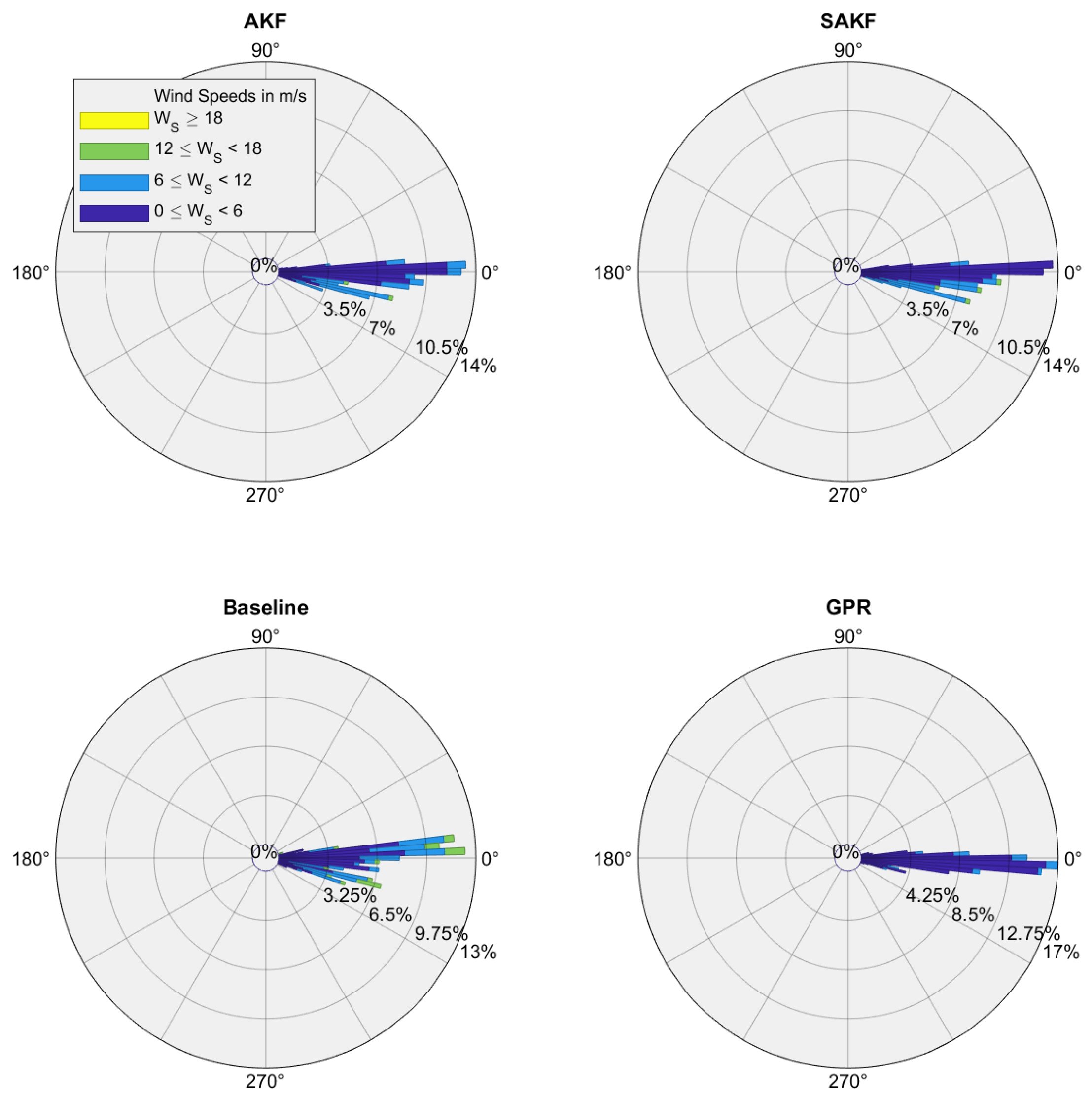
Figure 6 shows the rose diagrams of the wind direction estimation errors for the different methods. A rose diagram can be interpreted as an extension of the notion of a histogram to circular data. The quantities in the inner circumferences represent the amount of data, while the quantities in the outer circumference denote angles measured in degrees. In addition, the wind intensity is also represented with a colour legend. It can be observed that the angle estimation errors are close to 0 for all methods. Moreover, the GPR shows a lower spread in comparison to the rest of the approaches, and a minor wind intensity error.
In order to test if the performance of the GPR can be improved, some aircraft trajectories passing through the waypoints were added to the training dataset. Notice that this is a realistic assumption since all the added trajectories provide observations from an earlier instant of time. However, no significant improvement is observed in the performance of the GPR estimations by dispensing landing aircraft data. Thus, the covariance function is able to model the wind behaviour at the waypoints without the need to rely on the data located. Similarly, no significant improvement is observed when more non-landing aircraft data are added to the training dataset. Indeed, the numerical experiments indicate that between 1500 and 3000 observations are enough to achieve the best performance of the VWP estimation.
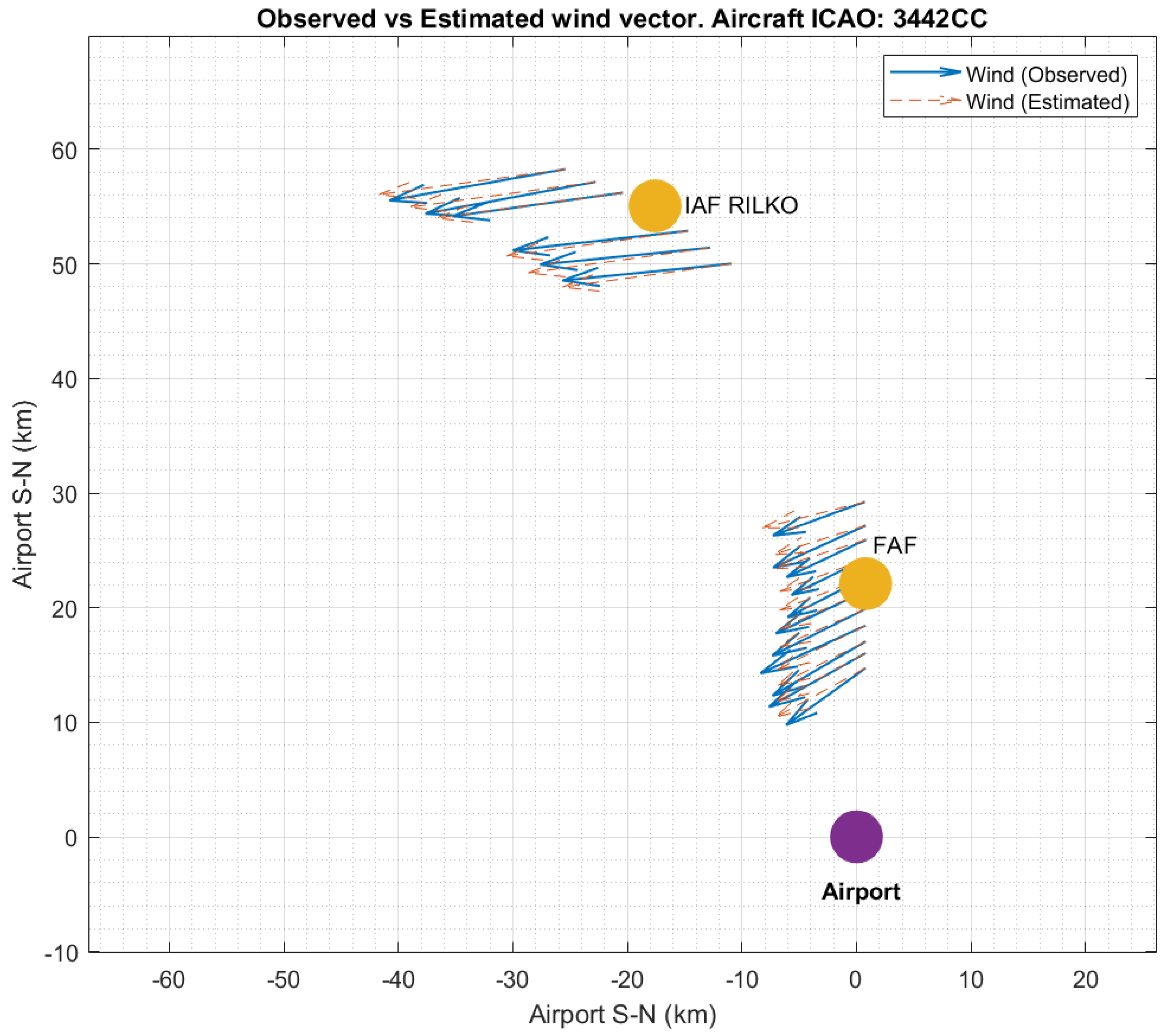
Figure 7 shows the VWP estimation obtained using the GPR assimilation technique together with the observed wind vector derived from aircraft 3442CC, which flies through the waypoints during a landing approach manoeuvre. It can be seen that the estimation and the observed measures agree.
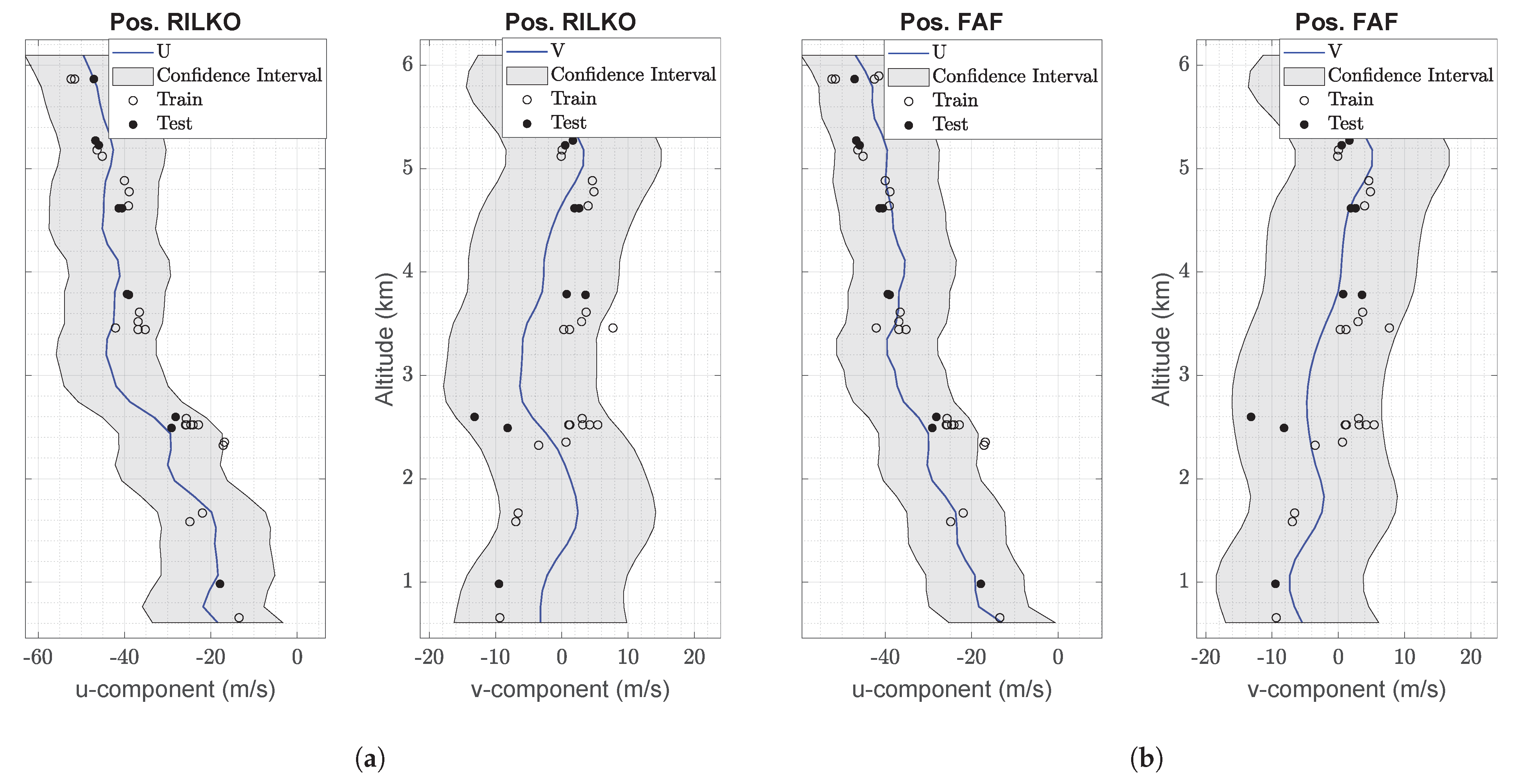
As mentioned in Section 2.4, one of the advantages of the GPR approach is that it allows a confidence interval for the estimations to be computed. Figure 8 shows a 95% confidence interval for the estimation of the wind components. Most of the test data fell in the confidence interval, meaning that the model suits the observed wind. It can be seen that this confidence interval is not constant. Indeed, it depends on the time and position where it is computed, which can be considered an advantage of the GPR technique, since the intervals adapt themselves depending on the degree of uncertainty of the estimation at each position. This feature confirms that the GPR is a very flexible model. One of the factors that most determine the interval length is the availability or not of close spatio-temporal data, although other factors are taken into account, such as the spread and variance of the available data.
4. Discussion and Conclusions
In this work, the capacity of GPR to construct vector wind profiles was assessed. The estimations can be carried out in real time, taking advantage of the large amount of constantly streamed airborne-transmitted data, sourcing a good choice for the assessment of data assimilation techniques.
The ability of the GPR method has been tested by estimating both the direction and intensity of the wind. The GPR method is able to adequately model the spatio-temporal wind correlations, including local variations. Moreover, the iterative version of the GPR method proposed in this paper is fast, allowing for data assimilation. For the sake of comparison, various vector wind profile estimations have also been conducted using state-of-the-art KF-based assimilation techniques. It has been proven that the best performance is achieved by the GPR method. Furthermore, the GPR method can accurately estimate the vector wind profiles, even when all the wind information coming from the landing aircraft is reserved for the testing phase, achieving a smooth estimation. Local variations between the two wind profiles located at the waypoints were also better represented by GPR. Additionally, the GPR method allows non-constant confidence intervals for the estimates to be computed, which reflect the uncertainty of the vector wind profile estimations at each spatio-temporal location.
The results may open new research lines, for example, enhancing the GPR for the data assimilation framework, using alternative multiple-output modelling, enabling it to perform short term predictions or online 3D wind field estimations. Furthermore, KF-based methods are not easily generalised for 3D grid formulations and require to be operated with huge matrices that may be hard to be computationally affordable, whereas GPR may be straightforwardly generalised with a low extra computation cost.
The method may be used in different aircraft performance studies, for climb and descent operations, and for general operational purposes. In conclusion, the research may contribute to the present and future of ATM, where accurate and on-demand wind information is essential.
Author Contributions
M.M., A.O., E.S. and J.S. contributed equally to this work. All authors have read and agreed to the published version of the manuscript.
Funding
This research was partially funded by the grants number TRA2017-91203-EXP and RTI2018-098471-B-C33 of the Spanish Government.
Institutional Review Board Statement
Not applicable.
Informed Consent Statement
Not applicable.
Data Availability Statement
The data used in this paper are property of ENAIRE, the Spanish National Air Navigation Service Provider, and are protected under a legal agreement. Contact ENAIRE ([email protected]) for access requirements.
Acknowledgments
The authors would like to thank Enrique Gismera Gómez, Ruth Otero Fraguas, and Iciar Sánchez Zorzano from ENAIRE for providing the data.
Conflicts of Interest
The authors declare no conflict of interest.
References
- Cook, A.; Rivas, D. Complexity Science in Air Traffic Management; Routledge: London, UK, 2016. [Google Scholar]
- Rodriguez-Sanz, A.; Cano, J.; Rubio Fernandez, B. Impact of weather conditions on airport arrival delay and throughput. Aircr. Eng. Aerosp. Technol. 2021, 94, 60–78. [Google Scholar] [CrossRef]
- Rapid Refresh (NOAA). Available online: https://rapidrefresh.noaa.gov (accessed on 16 May 2022).
- FAQ: Weather Delay (FAA). Available online: https://www.faa.gov/nextgen/programs/weather/faq (accessed on 16 May 2022).
- NextGen (FAA). Available online: https://www.faa.gov/nextgen (accessed on 16 May 2022).
- Dalmau, R.; Prats, X.; Baxley, B. Using broadcast wind observations to update the optimal descent trajectory in real-time. J. Air Transp. 2020, 28, 82–92. [Google Scholar] [CrossRef]
- Buelta, A.; Olivares, A.; Staffetti, E. Iterative learning control for precise aircraft trajectory tracking in continuous climb and descent operations. IEEE Trans. Intell. Transp. Syst. 2021, 1–11, early access article.. [Google Scholar] [CrossRef]
- De Jong, P.M.A.; van der Laan, J.J.; in ’t Veld, A.C.; van Paassen, M.M.; Mulder, M. Wind-profile estimation using airborne sensors. J. Aircr. 2014, 51, 1852–1863. [Google Scholar] [CrossRef]
- Pellerin, P. SESAR JU—Initial 4D “On Time”; ATC Global: London, UK, 2012. [Google Scholar]
- Reynolds, T.G.; McPartland, M.; Teller, T.; Troxel, S. Exploring wind information requirements for four dimensional trajectory-based operations. In Proceedings of the Eleventh USA/Europe Air Traffic Management Research and Development Seminar, Lisbon, Portugal, 23–26 June 2015. [Google Scholar]
- De Haan, S. High-resolution wind and temperature observations from aircraft tracked by Mode-S air traffic control radar. J. Geophys. Res. Atmos. 2011, 116, D10. [Google Scholar] [CrossRef]
- Robert, E.; De Smedt, D. Comparison of operational wind forecasts with recorded flight data. In Proceedings of the 10th USA/Europe Air Traffic Management Research and Development Seminar, Chicago, IL, USA, 10–13 June 2013. [Google Scholar]
- Sun, J.; Vû, H.; Ellerbroek, J.; Hoekstra, J.M. Weather field reconstruction using aircraft surveillance data and a novel meteo-particle model. PLoS ONE 2018, 13, e0205029. [Google Scholar] [CrossRef]
- Liu, T.; Xiong, T.; Thomas, L.; Liang, Y. ADS-B based wind speed vector inversion algorithm. IEEE Access 2020, 8, 150186–150198. [Google Scholar] [CrossRef]
- SWIM Project. Available online: https://www.eurocontrol.int/concept/system-wide-information-management (accessed on 16 May 2022).
- De Haan, S.; Stoffelen, A. Assimilation of high-resolution Mode-S wind and temperature observations in a regional NWP model for nowcasting applications. Weather Forecast. 2012, 27, 918–937. [Google Scholar] [CrossRef]
- Cardinali, C.; Isaksen, L.; Andersson, E. Use and impact of automated aircraft data in a global 4DVAR data assimilation system. Mon. Weather Rev. 2003, 131, 1865–1877. [Google Scholar] [CrossRef]
- 2019 by the Numbers (Flightradar24). Available online: https://www.flightradar24.com/blog/flightradar24s-2019-by-the-numbers/ (accessed on 16 May 2022).
- AMDAR Observing System. Available online: https://public.wmo.int/en/programmes/global-observing-system/amdar-observing-system (accessed on 16 May 2022).
- Strajnar, B. Validation of Mode-S meteorological routine air report aircraft observations. J. Geophys. Res. Atmos. 2012, 117, D23. [Google Scholar] [CrossRef]
- Marinescu, M.; Olivares, A.; Staffetti, E.; Sun, J. Wind profile estimation from aircraft derived data using Kalman filters and Gaussian process regression. In Proceedings of the 14th USA/Europe Air Traffic Management Research and Development Seminar, Virtual Event, 20–23 September 2021. [Google Scholar]
- Mondoloni, S. A multiple-scale model of wind-prediction uncertainty and application to trajectory prediction. In Proceedings of the 6th AIAA Aviation Technology, Integration, and Operations Conference, Wichita, KS, USA, 25–27 September 2006. [Google Scholar]
- Dalmau, R.; Pérez-Batlle, M.; Prats, X. Estimation and prediction of weather variables from surveillance data using spatio-temporal Kriging. In Proceedings of the 2017 IEEE/AIAA 36th Digital Avionics Systems Conference, St. Petersburg, FL, USA, 17–21 September 2017. [Google Scholar]
- Delahaye, D.; Puechmorel, S.; Vacher, P. Windfield estimation by radar track Kalman filtering and vector spline extrapolation. In Proceedings of the 22nd Digital Avionics Systems Conference, Indianapolis, IN, USA, 12–16 October 2003. [Google Scholar]
- De Leege, A.M.P.; van Paassen, M.M.; Mulder, M. Using automatic dependent surveillance-broadcast for meteorological monitoring. J. Aircr. 2013, 50, 249–261. [Google Scholar] [CrossRef]
- Sun, J.; Vû, H.; Ellerbroek, J.; Hoekstra, J.M. pyModeS: Decoding Mode-S surveillance data for open air transportation research. IEEE Trans. Intell. Transp. Syst. 2020, 21, 2777–2786. [Google Scholar] [CrossRef]
- Weston, K.J. Boundary layer climates. Q. J. R. Meteorol. Soc. 1988, 114, 1568. [Google Scholar] [CrossRef]
- Zoumakis, N.; Kelessis, A.G. Methodology for bulk approximation of the wind profile power-law exponent under stable stratification. Bound.-Layer Meteorol. 1991, 55, 199–203. [Google Scholar] [CrossRef]
- User’s Guide for Monthly Vector Wind Profile Mode. Available online: https://ntrs.nasa.gov/api/citations/20000011734/downloads/20000011734.pdf (accessed on 16 May 2022).
- Smith, O.; Adelfang, S. Wind profile models-Past, present and future for aerospace vehicle ascent design. In Proceedings of the 36th AIAA Aerospace Sciences Meeting and Exhibit, Reno, NV, USA, 12–15 January 1998. [Google Scholar]
- Kalman, R.E. A new approach to linear filtering and prediction problems. J. Basic Eng. 1960, 82, 35–45. [Google Scholar] [CrossRef] [Green Version]
- Bucy, R.S.; Joseph, P.D. Filtering for stochastic processes with applications to guidance. N. Y. Intersci. Publ. 1968, 17, 184–185. [Google Scholar]
- Chen, Z. Bayesian filtering: From Kalman filters to particle filters, and beyond. Statistics 2003, 182, 1–69. [Google Scholar]
- Talagrand, O. Assimilation of observations, an introduction. J. Meteorol. Soc. Jpn. Ser. II 1997, 75, 191–209. [Google Scholar] [CrossRef] [Green Version]
- Bishop, C.H.; Etherton, B.J.; Majumdar, S.J. Adaptive sampling with the ensemble transform Kalman filter. Part I: Theoretical aspects. Mon. Weather Rev. 2001, 129, 420–436. [Google Scholar] [CrossRef]
- Hunt, B.; Kostelich, E.; Szunyogh, I. Efficient data assimilation for spatiotemporal chaos: A local ensemble transform Kalman filter. Phys. D Nonlinear Phenom. 2005, 230, 112–126. [Google Scholar] [CrossRef] [Green Version]
- Rasmussen, C.; Williams, C. Gaussian Processes for Machine Learning; MIT Press: Cambridge, MA, USA, 2006. [Google Scholar]
- Martino, L.; Read, J. A joint introduction to Gaussian processes and relevance vector machines with connections to Kalman filtering and other kernel smoothers. Inf. Fusion 2021, 74, 17–38. [Google Scholar] [CrossRef]
- Wang, B.; Chen, T. Gaussian process regression with multiple response variables. Chemom. Intell. Lab. Syst. 2015, 142, 159–165. [Google Scholar] [CrossRef] [Green Version]
- Liu, H.; Cai, J.; Ong, Y.S. Remarks on multi-output Gaussian process regression. Knowl.-Based Syst. 2018, 144, 102–121. [Google Scholar] [CrossRef]
- Micchelli, C.A.; Xu, Y.; Zhang, H. Universal kernels. J. Mach. Learn. Res. 2006, 7, 2651–2667. [Google Scholar]
- Schölkopf, B.; Burges, C.J.; Smola, A.J. Advances in Kernel Methods; MIT Press: Cambridge, MA, USA, 1999. [Google Scholar]
- Bo, L.; Sminchisescu, C. Greedy block coordinate descent for large scale Gaussian process regression. In Proceedings of the Twenty-Fourth Conference on Uncertainty in Artificial Intelligence, Helsinki, Finland, 9–12 July 2008. [Google Scholar]
Figure 1.
Relationship between true airspeed, ground speed, and wind vectors.

Figure 2.
VWP estimation framework. The cyan trajectory represents the final approach path of an aircraft landing. Blue vertical lines represent the locations where wind profiles are estimated.
Figure 2.
VWP estimation framework. The cyan trajectory represents the final approach path of an aircraft landing. Blue vertical lines represent the locations where wind profiles are estimated.

Figure 3.
Realisations of different Gaussian processes generated by diverse covariance functions or kernel and represented as wind profiles.
Figure 3.
Realisations of different Gaussian processes generated by diverse covariance functions or kernel and represented as wind profiles.

Figure 4.
Estimated vector wind profiles obtained using different assimilation techniques along with the training and testing data available at 14:10 UTC. (a) Vector wind profile at RILKO IAF. (b) Vector wind profile at FAF waypoint.
Figure 4.
Estimated vector wind profiles obtained using different assimilation techniques along with the training and testing data available at 14:10 UTC. (a) Vector wind profile at RILKO IAF. (b) Vector wind profile at FAF waypoint.

Figure 5.
Wind speed and direction error boxplots for the different assimilation techniques.

Figure 6.
Rose diagrams of the wind direction estimation errors for the different methods.

Figure 7.
Comparison of estimated and observed wind vector when aircraft 3442CC flies through the waypoints RILKO IAF and FAF. The east-west and south-north directions are represented in the x and y axes, respectively.
Figure 7.
Comparison of estimated and observed wind vector when aircraft 3442CC flies through the waypoints RILKO IAF and FAF. The east-west and south-north directions are represented in the x and y axes, respectively.

Figure 8.
Confidence intervals for the VWP estimated using the GPR technique along with the training and testing data available at time 14:10 UTC. (a) Confidence interval for the VWP estimated at RILKO IAF waypoint. (b) Confidence interval for the VWP estimated at FAF waypoint.
Figure 8.
Confidence intervals for the VWP estimated using the GPR technique along with the training and testing data available at time 14:10 UTC. (a) Confidence interval for the VWP estimated at RILKO IAF waypoint. (b) Confidence interval for the VWP estimated at FAF waypoint.


Table 1.
Performance measures for the -components.
| Type | Variable | Baseline | AKF | SAKF | GPR |
|---|---|---|---|---|---|
| RMSE (m/s) | u | 6.2 | 4.8 | 5.0 | 3.1 |
| v | 6.0 | 5.1 | 5.1 | 2.9 | |
| Wind speed | 6.5 | 5.0 | 5.2 | 3.0 | |
| MAE (m/s) | u | 4.8 | 3.7 | 3.9 | 2.4 |
| v | 4.4 | 3.6 | 3.5 | 2.4 | |
| Wind speed | 5.0 | 3.8 | 3.9 | 2.2 |
Publisher’s Note: MDPI stays neutral with regard to jurisdictional claims in published maps and institutional affiliations. |
© 2022 by the authors. Licensee MDPI, Basel, Switzerland. This article is an open access article distributed under the terms and conditions of the Creative Commons Attribution (CC BY) license (https://creativecommons.org/licenses/by/4.0/).
Share and Cite
MDPI and ACS Style
Marinescu, M.; Olivares, A.; Staffetti, E.; Sun, J. On the Estimation of Vector Wind Profiles Using Aircraft-Derived Data and Gaussian Process Regression. Aerospace 2022, 9, 377. https://doi.org/10.3390/aerospace9070377
AMA Style
Marinescu M, Olivares A, Staffetti E, Sun J. On the Estimation of Vector Wind Profiles Using Aircraft-Derived Data and Gaussian Process Regression. Aerospace. 2022; 9(7):377. https://doi.org/10.3390/aerospace9070377
Chicago/Turabian StyleMarinescu, Marius, Alberto Olivares, Ernesto Staffetti, and Junzi Sun. 2022. "On the Estimation of Vector Wind Profiles Using Aircraft-Derived Data and Gaussian Process Regression" Aerospace 9, no. 7: 377. https://doi.org/10.3390/aerospace9070377
Note that from the first issue of 2016, this journal uses article numbers instead of page numbers. See further details here.