
A Novel Direct Optimization Framework for Hypersonic Waverider Inverse Design Methods


Abstract
:1. Introduction
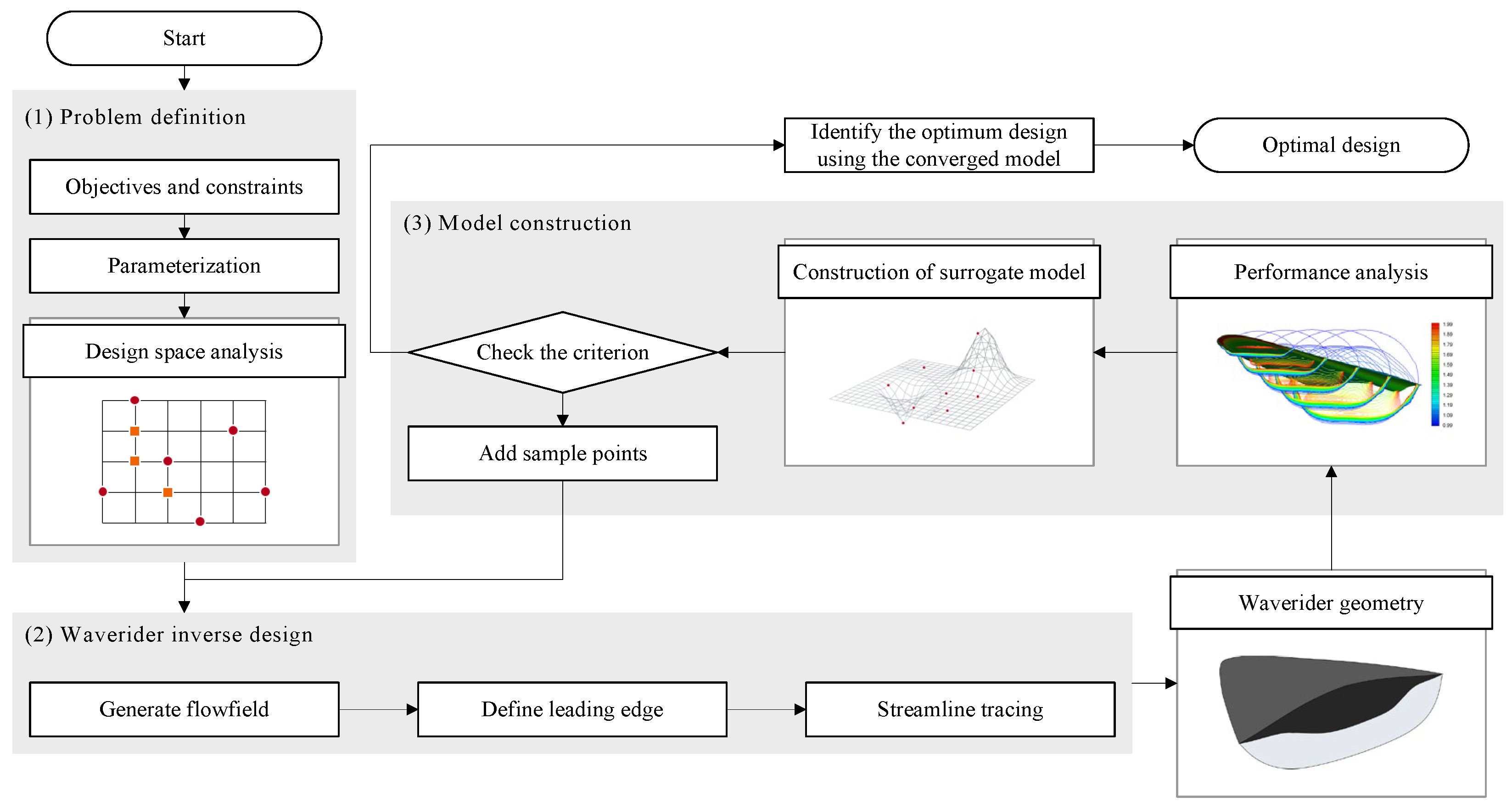
- (1)
- Generating the basic flow field
- (2)
- Defining the leading edge
- (3)
- Deriving the waverider configuration using the streamline tracing technique
2. Methodology
2.1. Direct Design Approach
2.2. Design Space Defining Methodology
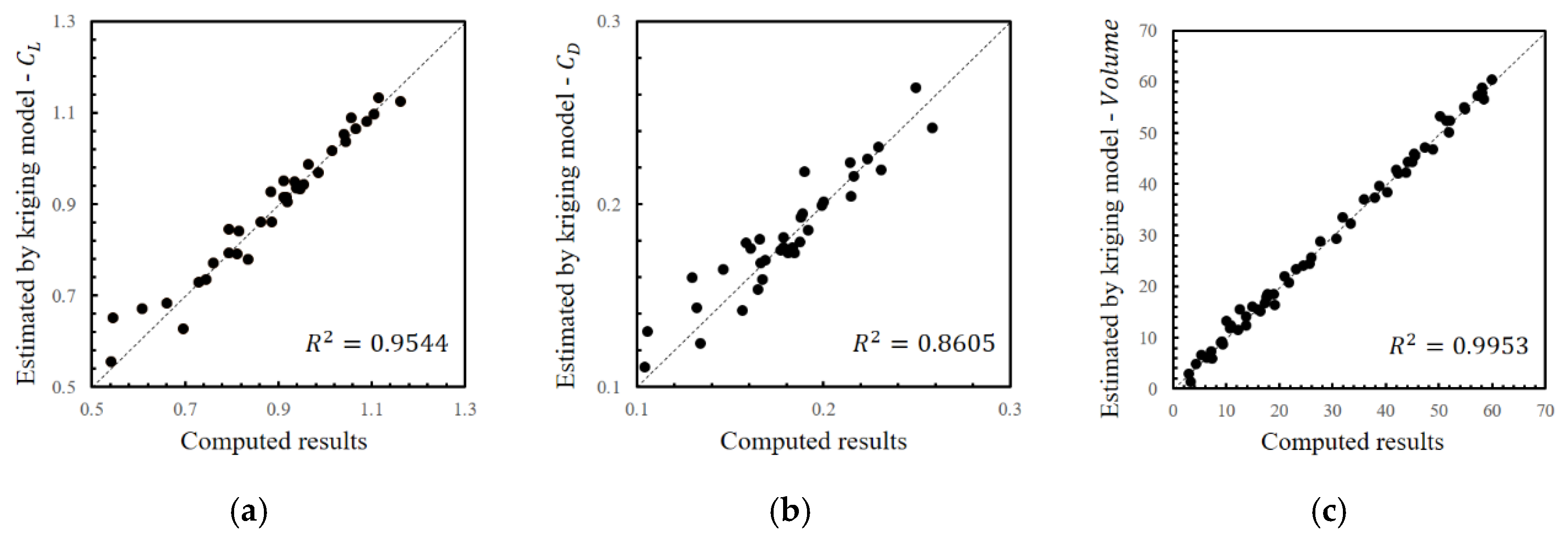
2.3. Performance Estimation Technique
3. Results and Discussion
3.1. Progress of Direct Optimization
3.1.1. Problem Definition
- ;
- ;
3.1.2. Model Construction
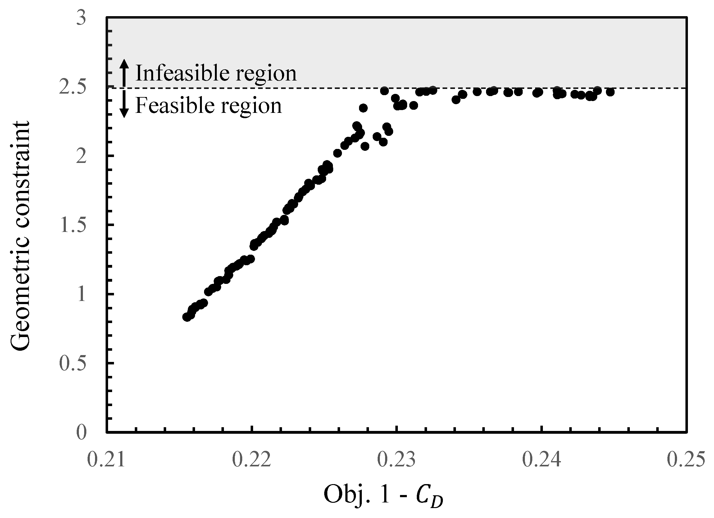
3.2. Design Optimization
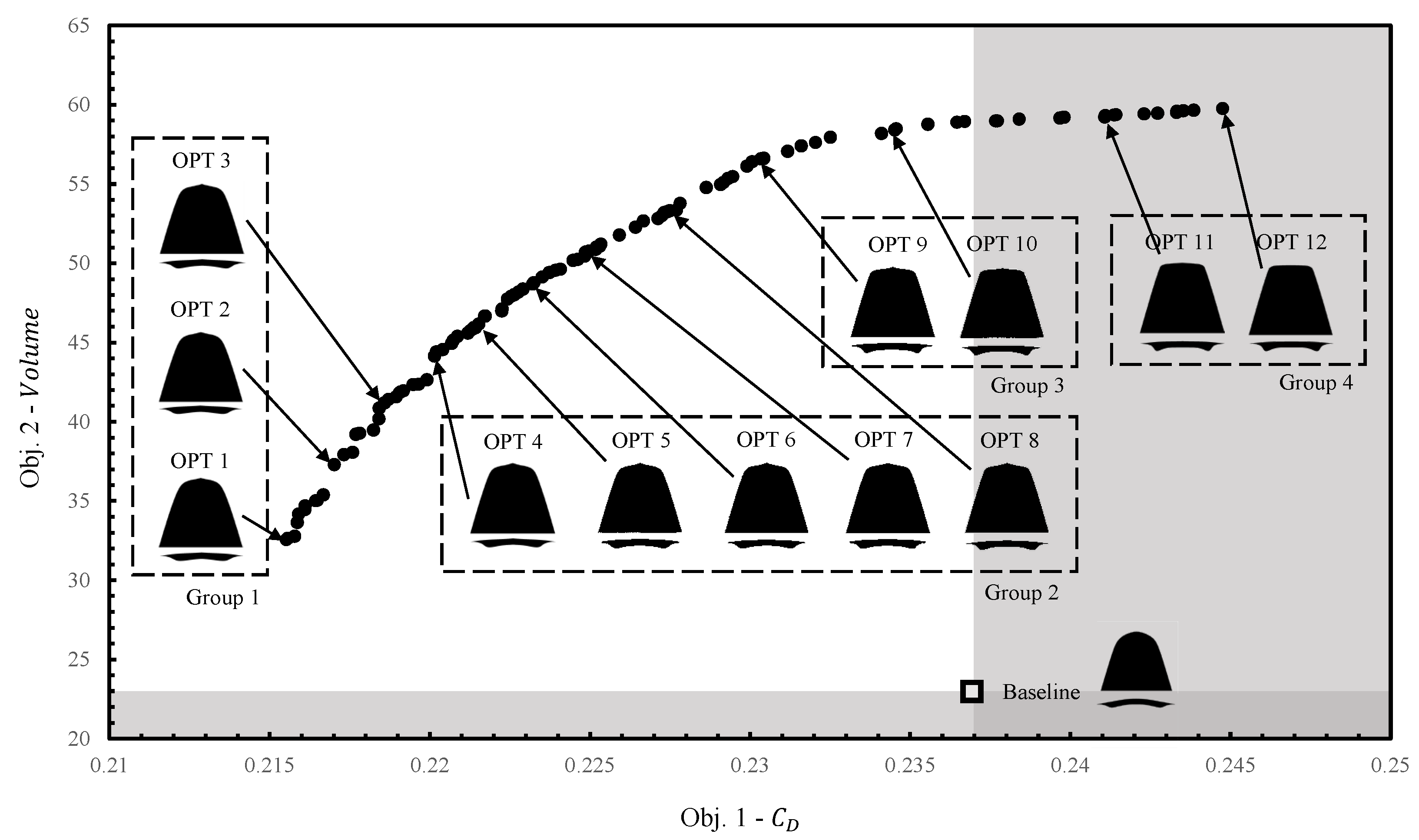
3.2.1. Optimized Results
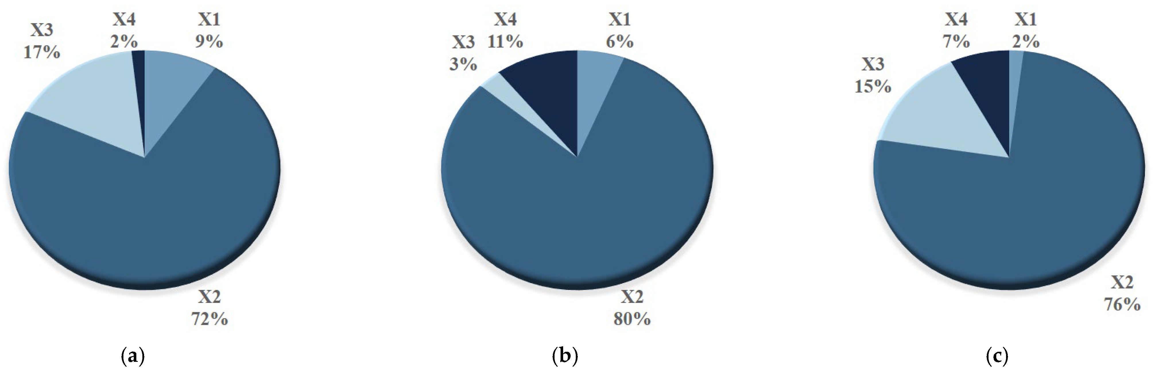
3.2.2. Decision Tree Analysis
4. Conclusions
- (1)
- We developed a general approach to define the design space, which can be applied to an arbitrary set of design parameters of a waverider using the osculating cone theory. To this end, the failure conditions of the waverider inverse design used in the literature were classified into two geometric relationships, which were mathematically analyzed and determined to be redundant. Based on the analysis, we obtained a discriminant formula that unifies the two conditions. The design space for the waverider can be derived by applying the discriminant formula to the design curves. We observed that the obtained design space was more accurately represented than the reference model based on the ad hoc relation;
- (2)
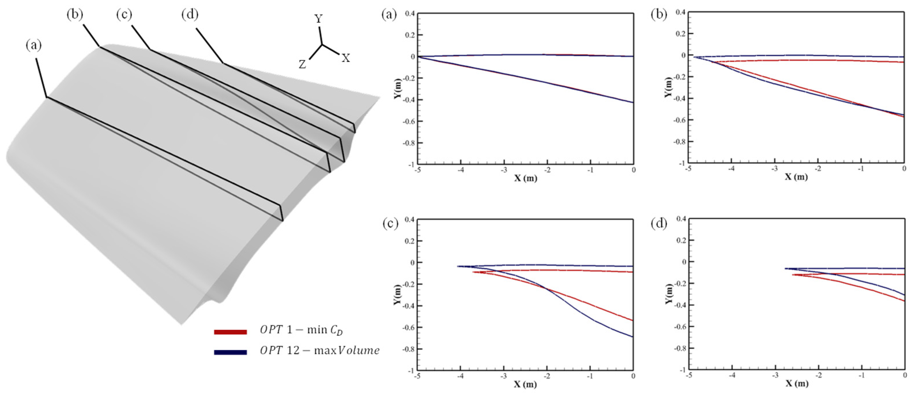
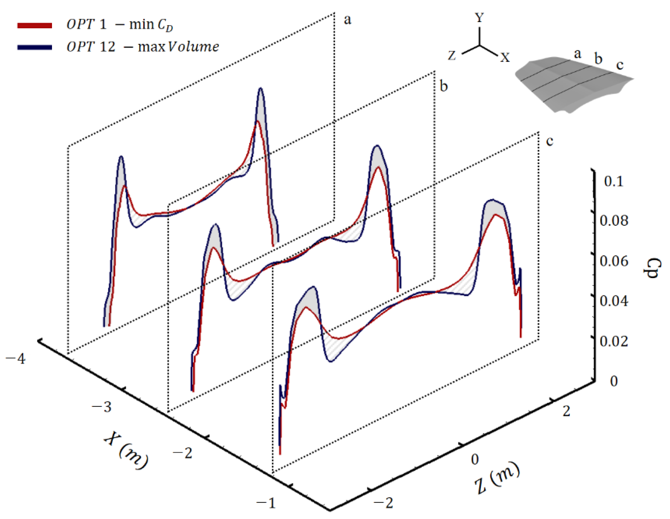
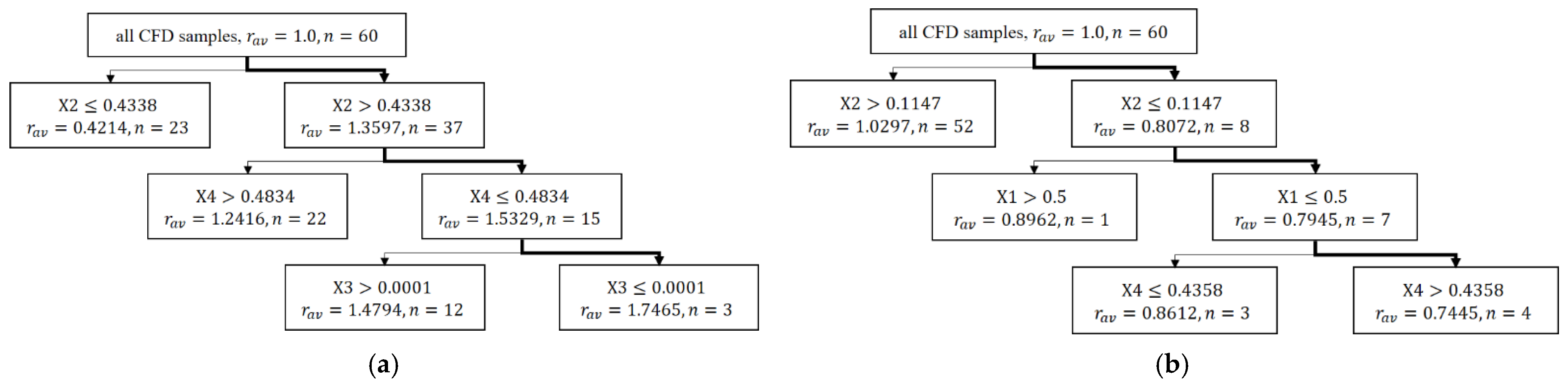
- Further, general characteristics of the waverider were derived using data mining methods, such as K-means clustering and decision tree analysis. The aerodynamic performance and the shape of the waverider were primarily affected by the curvature of the shockwave. The large curvature of the shockwave reduced the distance between the cone vertex of the osculating plane and the upper surface point. Consequently, the lower surface tends to approach the shockwave. As a result, the ends of the waverider protrude, and the internal volume increases. This protruding region increases the drag acting on the waverider. In summary, the waverider has an inherent geometric trade-off relationship between internal volume and drag;
- (3)
- In the proposed design framework, the aerodynamic performance of the aircraft was directly considered an objective or constraint during the design process, which is one of the primary strengths of the direct design method. The computational efficiency required for the direct design method was achieved using surrogate models derived from high-fidelity flow analyses.
Author Contributions
Funding
Institutional Review Board Statement
Informed Consent Statement
Data Availability Statement
Acknowledgments
Conflicts of Interest
Appendix A. Osculating Cone Theory

References
- Jackson, K.; Gruber, M.; Barhorst, T. The HIFIRE flight 2 experiment: An overview and status update. In Proceedings of the 45th AIAA/ASME/SAE/ASEE Joint Propulsion Conference & Exhibit, Denver, CO, USA, 2–5 August 2009. [Google Scholar] [CrossRef]
- Küchemann, D. Hypersonic aircraft and their aerodynamic problems. Prog. Aerosp. Sci 1965, 6, 271–353. [Google Scholar] [CrossRef]
- Nonweiler, T.R. Aerodynamic problems of Manned Space Vehicles. RAeS 1959, 63, 521–528. [Google Scholar] [CrossRef]
- Ding, F.; Liu, J.; Shen, C.-b.; Liu, Z.; Chen, S.-h.; Fu, X. An overview of research on Waverider Design methodology. Acta Astronaut. 2017, 140, 190–205. [Google Scholar] [CrossRef]
- Jones, J.G.; Moore, K.C.; Pike, J.; Roe, P.L. A method for designing lifting configurations for high supersonic speeds, using axisymmetric flow fields. Ing. Arch. 1968, 37, 56–72. [Google Scholar] [CrossRef]
- Rasmussen, M.L. Waverider Configurations Derived from Inclined Circular and Elliptic Cones. J. Spacecr. Rocket. 1980, 17, 537–545. [Google Scholar] [CrossRef]
- Sobieczky, H.; Dougherty, F.C.; Jones, K.D. Hypersonic Waverider Design from Given Shock Waves. In Proceedings of the First International Hypersonic Waverider Symposium, College Park, MD, USA, 17–19 October 1990. [Google Scholar]
- Chen, L.; Guo, Z.; Deng, X.; Hou, Z.; Wang, W. Waverider configuration design with variable shock angle. IEEE Access 2019, 7, 42081–42093. [Google Scholar] [CrossRef]
- Zheng, X.; Li, Y.; Zhu, C.; You, Y. Multiple osculating cones’ waverider design method for ruled shock surfaces. AIAA J. 2019, 58, 854–866. [Google Scholar] [CrossRef]
- Liebeck, R.H. Subsonic airfoil design. In Applied Computational Aerodynamics; Henne, P.A., Ed.; Progress in Astronautics and Aeronautics: New York, NY, USA, 1990; Volume 125, pp. 133–165. [Google Scholar] [CrossRef]
- Labrujere, T.E.; Slooff, J.W. Computational methods for the aerodynamic design of aircraft components. Annu. Rev. Fluid Mech. 1993, 25, 183–214. [Google Scholar] [CrossRef]
- Takashima, N. Optimization of Waverider—Based Hypersonic Vehicle Designs. Ph.D. Thesis, University of Maryland, College Park, MD, USA, 1997. [Google Scholar]
- Kontogiannis, K.; Sóbester, A.; Taylor, N. Efficient Parameterization of Waverider Geometries. J. Aircr. 2017, 54, 890–901. [Google Scholar] [CrossRef] [Green Version]
- Lobbia, M.A. Multidisciplinary Design Optimization of Waverider-Derived Crew Reentry Vehicles. J. Spacecr. Rocket. 2017, 54, 233–245. [Google Scholar] [CrossRef]
- Lobbia, M.A. Rapid Supersonic/Hypersonic Aerodynamics Analysis Model for arbitrary geometries. J. Spacecr. Rocket. 2017, 54, 315–322. [Google Scholar] [CrossRef]
- Goldberg, D.E. Genetic Algorithms in Search, Optimization and Machine Learning; Addison-Wesley Longman Publishing Co., Inc.: Boston, MA, USA, 1989. [Google Scholar]
- Fonseca, C.M.; Fleming, P.J. Genetic Algorithms for Multiobjective Optimization: FormulationDiscussion and Generalization. ICGA 1993, 93, 416–423. [Google Scholar] [CrossRef]
- Park, J.-S. Optimal latin-hypercube designs for computer experiments. J. Stat. Plan. Inference 1994, 39, 95–111. [Google Scholar] [CrossRef]
- Park, S.H.; Lee, J.E.; Kwon, J.H. Preconditioned Hlle method for flows at all Mach numbers. AIAA J. 2006, 44, 2645–2653. [Google Scholar] [CrossRef]
- Hong, Y.; Lee, D.; Yee, K.; Park, S.H. Enhanced high-order scheme for high-resolution rotorcraft flowfield analysis. AIAA J. 2022, 60, 144–159. [Google Scholar] [CrossRef]
- Lockman, W.K.; Lawrence, S.L.; Cleary, J.W. Flow over an all-body hypersonic aircraft—Experiment and Computation. J. Spacecr. Rocket. 1992, 29, 7–15. [Google Scholar] [CrossRef]
- Martin, J.D.; Simpson, T.W. Use of Kriging models to approximate deterministic computer models. AIAA J 2005, 43, 853–863. [Google Scholar] [CrossRef]
- Jones, D.R.; Schonlau, M.; Welch, W.J. Efficient Global Optimization of Expensive Black-Box Functions. J. Glob. Optim. 1998, 13, 455–492. [Google Scholar] [CrossRef]
- Pasquale, M.S. Commercial Airplane Design Principles, 1st ed.; Elsevier: Amsterdam, The Netherlands, 2014; pp. 487–495. [Google Scholar] [CrossRef]
- Lee, S.; Yee, K.; Rhee, D.-H. Optimization of the array of film-cooling holes on a high-pressure turbine nozzle. J. Propuls. Power 2017, 33, 234–247. [Google Scholar] [CrossRef]
- Jeong, S.; Chiba, K.; Obayashi, S. Data mining for aerodynamic design space. J. Aeros. Compt. Inf. Commun 2005, 2, 452–469. [Google Scholar] [CrossRef] [Green Version]
- Lloyd, S. Least squares quantization in PCM. IEEE Trans. Inf. Theory 1982, 28, 129–137. [Google Scholar] [CrossRef] [Green Version]
- Sugimura, K.; Obayashi, S.; Jeong, S. Multi-objective optimization and design rule mining for an aerodynamically efficient and stable centrifugal impeller with a vaned diffuser. Eng. Optim. 2010, 42, 271–293. [Google Scholar] [CrossRef]


| Cases | Grid Size | ||
|---|---|---|---|
| Coarse 1 | |||
| Coarse 2 | |||
| Moderate | |||
| Fine |
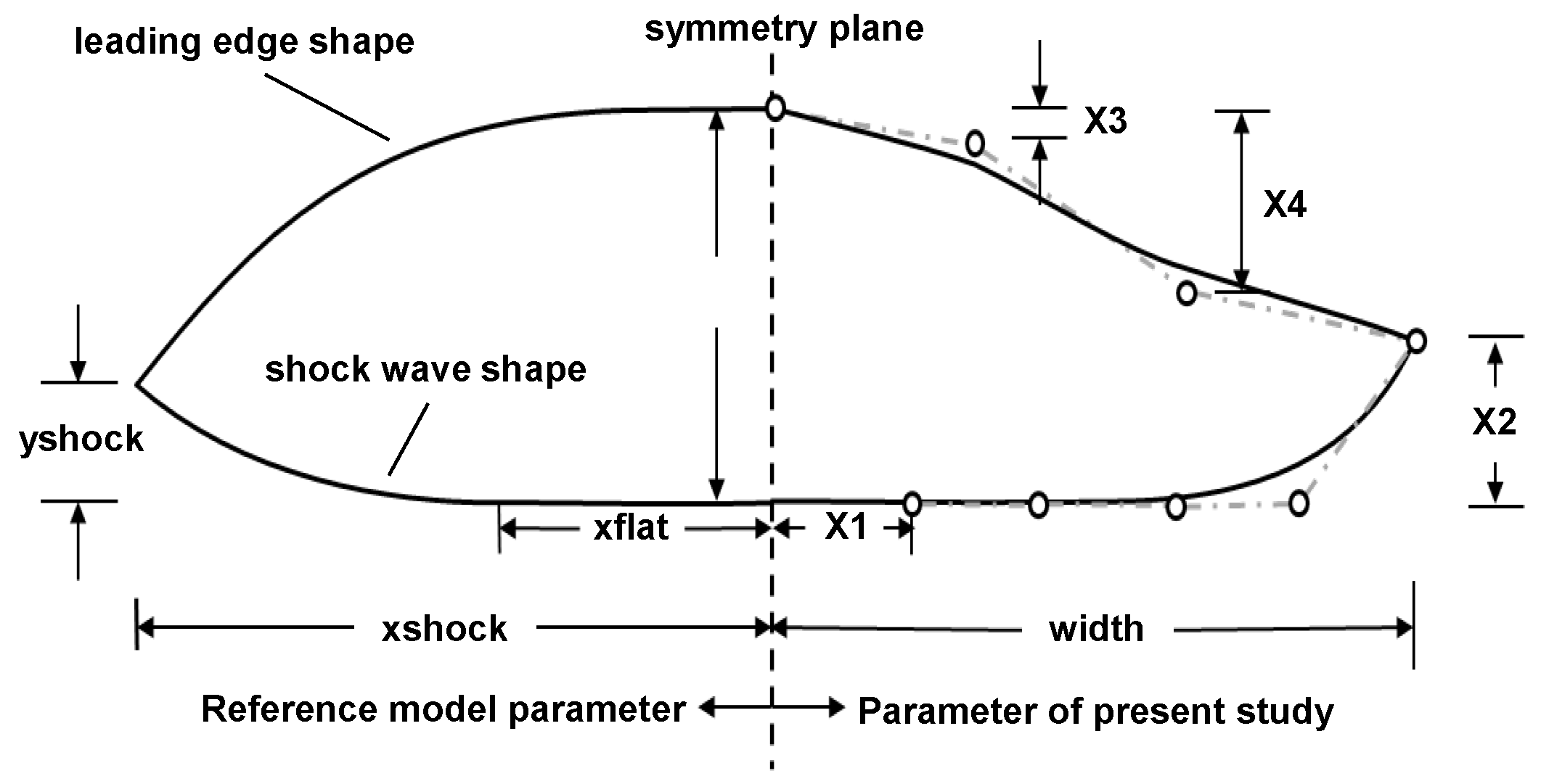
| Design Variable | Description |
|---|---|
| Flat region of the shockwave curve normalized with the width | |
| Height of the shockwave curve normalized with the height | |
| Vertical distance from the upper surface normalized with the | |
| Vertical distance from the upper surface normalized with the |
| X1 | X2 | X3 | X4 | Constraint | ||
|---|---|---|---|---|---|---|
| Group 1 | OPT 1 | 0.002 | 0.828 | 0.306 | 0.183 | 0.83 |
| OPT 2 | 0.051 | 0.824 | 0.351 | 0.198 | 1.02 | |
| OPT 3 | 0.088 | 0.826 | 0.393 | 0.184 | 1.19 | |
| Group 2 | OPT 4 | 0.119 | 0.826 | 0.418 | 0.194 | 1.37 |
| OPT 5 | 0.142 | 0.826 | 0.430 | 0.200 | 1.52 | |
| OPT 6 | 0.166 | 0.825 | 0.442 | 0.202 | 1.70 | |
| OPT 7 | 0.186 | 0.828 | 0.431 | 0.191 | 1.88 | |
| OPT 8 | 0.217 | 0.829 | 0.419 | 0.186 | 2.21 | |
| Group 3 | OPT 9 | 0.230 | 0.849 | 0.418 | 0.084 | 2.41 |
| OPT 10 | 0.225 | 0.881 | 0.317 | 0.020 | 2.44 | |
| Group 4 | OPT 11 | 0.226 | 0.885 | 0.168 | 0.044 | 2.47 |
| OPT 12 | 0.226 | 0.882 | 0.034 | 0.001 | 2.46 |
Publisher’s Note: MDPI stays neutral with regard to jurisdictional claims in published maps and institutional affiliations. |
© 2022 by the authors. Licensee MDPI, Basel, Switzerland. This article is an open access article distributed under the terms and conditions of the Creative Commons Attribution (CC BY) license (https://creativecommons.org/licenses/by/4.0/).
Share and Cite
Son, J.; Son, C.; Yee, K. A Novel Direct Optimization Framework for Hypersonic Waverider Inverse Design Methods. Aerospace 2022, 9, 348. https://doi.org/10.3390/aerospace9070348
Son J, Son C, Yee K. A Novel Direct Optimization Framework for Hypersonic Waverider Inverse Design Methods. Aerospace. 2022; 9(7):348. https://doi.org/10.3390/aerospace9070348
Chicago/Turabian StyleSon, Jiwon, Chankyu Son, and Kwanjung Yee. 2022. "A Novel Direct Optimization Framework for Hypersonic Waverider Inverse Design Methods" Aerospace 9, no. 7: 348. https://doi.org/10.3390/aerospace9070348