MC-New: A Program to Calculate Newtonian Aerodynamic Coefficients Based on Monte-Carlo Integration

Abstract

A computer program, MC-New, to calculate Newtonian aerodynamics is presented. The aerodynamic coefficients of a geometry expressed by an analytic function are calculated in a Monte-Carlo integration manner, in which the local forces on the randomly chosen sample points are summed up. The verification study and the accuracy analysis show that the program can provide good approximations of exact solutions. The example results of the parametric study on the Apollo-like entry capsule geometry are presented, showing the potential capability of the MC-New program as an efficient open-source tool for designing hypersonic vehicles.

1. Introduction

It is known that the Newtonian theory gives a good approximation for the aerodynamic coefficients of an object in the hypersonic flowfield with a high Mach number [1]. Under the Newtonian theory, pressure coefficients on a surface due to fluid impingement can be calculated in a simple way; the pressure coefficients from the Newtonian theory depend only on an angle between the flow direction and the surface’s normal direction, and it does not need information on the flowfield around the surface. Of course, for accurate predictions of the aerodynamic coefficients, it is necessary to simulate the flowfield including physics that can alter the pressure distribution on the surface, such as viscosity, thermal excitations, chemical reactions, and so on [2,3]. However, Computational Fluid Dynamics computations considering these complex physics are generally time-consuming. Even though the prediction accuracies are degraded, simpler methods, such as the Newtonian theory, are often preferred, particularly at the initial stage of designing a hypersonic space vehicle.

When the geometries of the hypersonic space vehicles can be expressed by mathematical functions, the total aerodynamic forces working on the capsule can be obtained analytically by integrating the Newtonian pressure coefficients over the surface. However, when the vehicle has an angle-of-attack against the freestream direction, the analytical integrations become difficult, and the aid of numerical integration methods is needed [4,5].

There are some computational programs that employ Newtonian theory to calculate the aerodynamics coefficients of hypersonic vehicles [6,7,8,9]. These programs calculate the surface integral of the force by summing up the forces on triangular elements that spread over the vehicle’s surfaces. Such panel methods usually require generating a computational mesh system on the vehicle’s surfaces. One can have more accurate solutions when using more finely resolved mesh systems that require larger storage memory size. Therefore, in spite of the simplicity of the Newtonian theory, panel methods to calculate the Newtonian aerodynamic coefficients still require a large working time to generate the computational mesh system, and large computer memory to store the mesh point data. Moreover, in the panel methods, it is difficult to clearly distinguish the areas visible and invisible from the upstream when panels cross the boundary. It may cause inaccuracy in the results because the different formulas of pressure coefficients should be used in the visible and invisible areas under the Newtonian theory.

In the present study, a computational program, MC-New, that calculates Newtonian aerodynamic coefficients based on a meshless Monte-Carlo integration method, which is free from a computational mesh generation procedure, has been developed. For a combination of simple geometries, the total aerodynamic coefficients are calculated by a superposition of coefficients for each geometry. The intersections between the different geometries are automatically calculated in the program from the several parameters input by users so that one can perform parametric studies of the geometric parameters more effectively. The aerodynamic coefficients are evaluated as a sum of local pressure force components on the sample points, which are randomly distributed on the surface. The visibility from the upstream of the sample points is judged by the direction of the surface normal vector, and the local pressure coefficients of the points are determined by the Newtonian theory. Because the accuracy of the solutions depends on the total number of sample points that are randomly chosen, one can simply improve the accuracy by adding sample points on the existing results. In the paper, the mathematical formulation used in MC-New is explained, and the developed code is verified by comparing the calculated drag coefficients with the exact solutions for a sphere, a cone, a sphere-cone, and a cylinder. Then, the developed code is further verified for a case of combined geometries with angle-of-attacks, and the accuracy of the code is discussed. Lastly, as an example of the application of MC-New program to a hypersonic vehicle design, a parametric study of the Apollo-like geometry on the aerodynamic characteristics is presented.

2. Methods of Calculation

2.1. Aerodynamic Coefficients Based on Newtonian Theory

According to the Newtonian theory [1], when a fluid element impinges on the wall, the fluid element loses the momentum component in the direction normal to the wall and exerts a force on the wall whose magnitude is equivalent to the momentum loss, as shown in the schematic in Figure 1.

When the mass flow rate is $\dot{m}$ and the freestream speed is $V$, the force $F_n$ exerting on the windward side of a flat plate is then given by

$$F_{n \mathrm{wind}}={(\dot{m}V)}_n,$$

(1)

and

$$F_{n \mathrm{lee}}=0,$$

(2)

on the leeward wall because the flow does not go around according to the Newtonian theory [1]. The normal component of momentum passing through an area $A$ in a unit time is given by

$${(\dot{m}V)}_n=\rho V_n^{2}A,$$

(3)

where $V_n$ is the normal component of the velocity and given by the dot product of the velocity vector $V={\left[V_x\hspace{0.33em}{V}_y\hspace{0.33em}{V}_z\right]}^t$ and the unit normal vector $n={[n_x\hspace{0.33em}{n}_y\hspace{0.33em}{n}_z]}^t$;

$$V_n=V\cdot n.$$

(4)

Then, the pressure on an inclined flat plate with the area of $A$ in a flow with the velocity $V={\left[V\hspace{0.33em}0\hspace{0.33em}0\right]}^t$ parallel to the x-axis can be calculated by

$$p=\frac{F_n}{A}=\rho V^2{\left[\min (0,n_x)\right]}^2,$$

(5)

in magnitude because the surface in the windward side has negative values of $n_x$, and when $n_x$ is positive, the pressure is zero. The pressure components in $x$, $y$ and $z$ direction are then given by multiplying the normal vector by the pressure magnitude,

$$p=pn.$$

(6)

The force exerted on an arbitrary three-dimensional surface can be calculated by integrating the local pressure over the surface $S$,

$$F={\displaystyle {\int }_{S}p}ndA.$$

(7)

Then, the drag and the lift coefficients are given by

$$C_D=\frac{F_x}{\frac{1}{2}\rho V^2{A}_{\mathrm{ref}}}=\frac{2}{A_{\mathrm{ref}}}{\displaystyle {\int }_S{\left[\min (0,n_x)\right]}^2}{n}_{x}dA,$$

(8)

$$C_{L,y}=\frac{F_y}{\frac{1}{2}\rho V^2{A}_{\mathrm{ref}}}=\frac{2}{A_{\mathrm{ref}}}{\displaystyle {\int }_S{\left[\min (0,n_x)\right]}^2}{n}_{y}dA,$$

(9)

and

$$C_{L,z}=\frac{F_z}{\frac{1}{2}\rho V^2{A}_{\mathrm{ref}}}=\frac{2}{A_{\mathrm{ref}}}{\displaystyle {\int }_S{\left[\min (0,n_x)\right]}^2}{n}_{z}dA,$$

(10)

respectively.

2.2. Aerodynamic Coefficients on Surfaces with Pitch and Yaw Angle

Let a position vector of a point on a space vehicle’s body surface in the cartesian space coordinate be expressed by

$$r={[x\hspace{0.33em}y\hspace{0.33em}z]}^t.$$

(11)

Now, consider rotational transformations

$$R(\alpha )=\left[\begin{array}{ccc}\cos \alpha & 0& -\sin \alpha \\ 0& 1& 0\\ \sin \alpha & 0& \cos \alpha \end{array}\right]$$

(12)

and

$$R(\beta )=\left[\begin{array}{ccc}\cos \beta & -\sin \beta & 0\\ \sin \beta & \cos \beta & 0\\ 0& 0& 1\end{array}\right]$$

(13)

where $R_y(\alpha )$ and $R_z(\beta )$ are rotations about the $y$-axis and the $z$-axis and, respectively. When a space vehicle is placed in the space coordinate with the pitch angle of $\alpha$ and the yaw angle of $\beta$, as shown in Figure 2, the position vectors in the space coordinate are transformed into vectors in the body-fixed coordinates by

$$\tilde{\mathbf{r}}={[\tilde{x}\hspace{0.33em}\tilde{y}\hspace{0.33em}\tilde{z}]}^t=R_y(\alpha )R_z(\beta )r.$$

(14)

Conversely, position vectors defined in the body-fixed coordinates are expressed by

$$r=R_z^{-1}(\beta )R_y^{-1}(\alpha )\tilde{\mathbf{r}}$$

(15)

in the space coordinate. Similarly, when the normal vector is given in the body-fixed coordinates by

$$\tilde{\mathbf{n}}={[{\tilde{n}}_x\hspace{0.33em}{\tilde{n}}_y\hspace{0.33em}{\tilde{n}}_z]}^t,$$

(16)

the expression in the space coordinate is

$$n=R_z^{-1}(\beta )R_y^{-1}(\alpha )\tilde{\mathbf{n}},$$

(17)

that is,

$$\left[\begin{array}{c}{n}_x\\ n_y\\ n_z\end{array}\right]=\left[\begin{array}{ccc}\cos \beta & \sin \beta & 0\\ -\sin \beta & \cos \beta & 0\\ 0& 0& 1\end{array}\right]\left[\begin{array}{ccc}\cos \alpha & 0& \sin \alpha \\ 0& 1& 0\\ -\sin \alpha & 0& \cos \alpha \end{array}\right]\left[\begin{array}{c}{\tilde{n}}_x\\ {\tilde{n}}_y\\ {\tilde{n}}_z\end{array}\right].$$

(18)

Then, the aerodynamic coefficients of the vehicle in the flowfield with the freestream velocity, $V={\left[V\hspace{0.33em}0\hspace{0.33em}0\right]}^t$, can be obtained by substituting Equation (18) into Equations (8)–(10);

$${[C_D,C_{L_y},C_{L_z}]}^t=\frac{2}{A_{\mathrm{ref}}}{\displaystyle {\int }_S{\left[\min (0,n_x)\right]}^2}{[n_x,n_y,n_z]}^{t}dA.$$

(19)

The local pressure and the local force vector in the body-fixed coordinate are given by

$$\tilde{p}=p\tilde{n},$$

(20)

and

$$d\tilde{F}=p\tilde{n}dA,$$

(21)

respectively, because the magnitude of local pressure does not change by the coordinate transformation. Then, using the pressure expressed by Equation (5), the aerodynamic coefficients for the forces in the three axis directions of the body-fixed coordinate, $C_A$, $C_S$, and $C_N$ are calculated by

$${[C_A,C_S,C_N]}^t=\frac{2}{A_{\mathrm{ref}}}{\displaystyle {\int }_S{\left[\min (0,n_x)\right]}^2}{[{\tilde{n}}_x,{\tilde{n}}_y,{\tilde{n}}_z]}^{t}dA.$$

(22)

Additionally, the moment coefficients about a point $\tilde{q}$ in the body-fixed coordinate can be obtained by

$${\tilde{\mathbf{C}}}_m=\frac{1}{\frac{1}{2}\rho V^2{A}_{\mathrm{ref}}{l}_{\mathrm{ref}}}{\displaystyle {\int }_S(\tilde{\mathbf{r}}-\tilde{\mathbf{q}})}\times (p\tilde{\mathbf{n}})dA,$$

(23)

that is,

$${[C_{m,\tilde{x}},C_{m,\tilde{y}},C_{m,\tilde{z}}]}^t=\frac{2}{A_{\mathrm{ref}}{l}_{\mathrm{ref}}}{\displaystyle {\int }_S{\left[\min (0,n_x)\right]}^2}{[{\tilde{d}}_x,{\tilde{d}}_y,{\tilde{d}}_z]}^t\times {[{\tilde{n}}_x,{\tilde{n}}_y,{\tilde{n}}_z]}^{t}dA$$

(24)

where $\tilde{\mathbf{d}}=\tilde{\mathbf{r}}-\tilde{\mathbf{q}}$.

Figure 2. Coordinate transformation in the present study, when a space vehicle is placed in the space coordinate with the pitch angle of $\alpha$ and the yaw angle of $\beta$.

Figure 2. Coordinate transformation in the present study, when a space vehicle is placed in the space coordinate with the pitch angle of $\alpha$ and the yaw angle of $\beta$.

2.3. Monte-Carlo Integration

Now, consider a surface in the body-fixed coordinate being expressed by a parametric representation

$$\tilde{\mathbf{r}}(\eta ,\xi )={[\tilde{x}(\eta ,\xi )\hspace{0.33em}\tilde{y}(\eta ,\xi )\hspace{0.33em}\tilde{z}(\eta ,\xi )]}^t.$$

(25)

Then, the normal vector of the surface in the transformed coordinates is given by

$$\tilde{\mathbf{N}}={[{\tilde{N}}_x\hspace{0.33em}{\tilde{N}}_y\hspace{0.33em}{\tilde{N}}_z]}^t={\tilde{\mathbf{r}}}_{\eta }\times {\tilde{\mathbf{r}}}_{\xi }.$$

(26)

Because the magnitude of the local normal vector does not change by coordinate transformation, the integral Equation (7) can be written in terms of parameters $\eta$ and $\xi$;

$$F={\displaystyle {\int }_{S}p}ndA={\displaystyle \int {\displaystyle {\int }_{R}p}}n(\tilde{\mathbf{r}}(\eta ,\xi ))|{\tilde{\mathbf{r}}}_{\eta }\times {\tilde{\mathbf{r}}}_{\xi }|d\eta d\xi ,$$

(27)

and the Equation (19) by

$${[C_D,C_{L_y},C_{L_z}]}^t=\frac{2}{A_{\mathrm{ref}}}{\displaystyle \int {\displaystyle {\int }_R{\left[\min (0,n_x)\right]}^2}}{[n_x,n_y,n_z]}^t|{\tilde{\mathbf{r}}}_{\eta }\times {\tilde{\mathbf{r}}}_{\xi }|d\eta d\xi ,$$

(28)

where $A_R$ is the area of the parametric domain given by

$$A_R={\displaystyle \int {\displaystyle {\int }_{R}d}}\eta d\xi .$$

(29)

To evaluate the integrals in Equation (26), the present study employs a Monte-Carlo integration method; generate a sample point by a uniform random sampling in the parametric domain $R$, ${\eta }_{\min }<\eta <{\eta }_{\max }$ and ${\xi }_{\min }<\xi <{\xi }_{\max }$, calculate the normal vector on the sample points according to Equation (26), and then the integral Equation (28) is approximately calculated by

$${[C_D,C_{L_y},C_{L_z}]}^t\approx \frac{2}{A_{\mathrm{ref}}}\frac{A_R}{N}{\displaystyle \sum _{i=1}^N{\left[\min (0,n_{x i})\right]}^2}{[n_{x i},n_{y i},n_{z i}]}^t|N_i|,$$

(30)

where $N$ is the total number of sample points. The integrals in Equations (23) and (24) are also evaluated similarly.

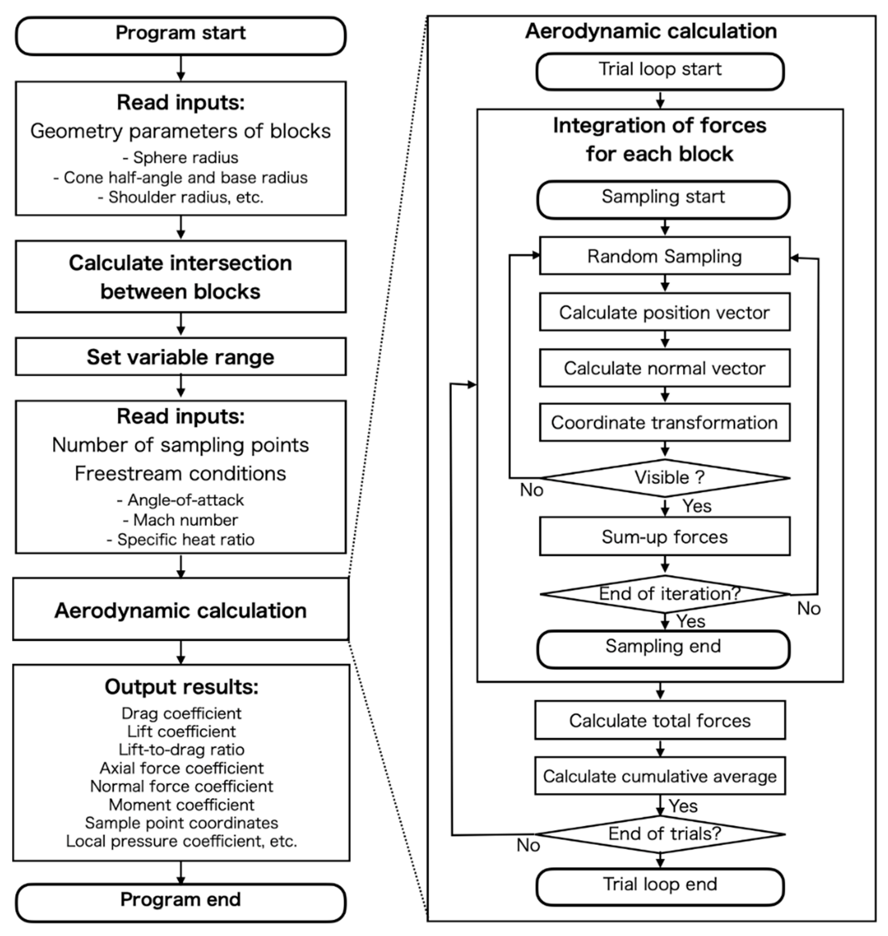
2.4. Computation Process

The computation process flow chart of the MC-New program is shown in Figure 3. The detailed descriptions of the usage are available in the document of Supplementary Materials.

The flow of preprocessing is as follows. The geometry is divided into several blocks. Each block is either a sphere, a cone, a shoulder (torus), a cylinder, or a circle. After reading the number of blocks, the geometric parameters are read; the radius of the sphere, the half-angle of the cone, and so on. The intersections between adjacent blocks are then calculated, and the parameter ranges for surface integration are consequently determined.

Once the integration ranges are determined, the aerodynamics calculation process starts. For each block, the aerodynamic coefficients are calculated as follows. Two parameters, $\eta$ and $\xi$, are determined by uniform random number sampling to calculate a point position vector expressed by Equation (25). The normal vector calculated for the sample point is rotated by the input pitch and yaw angles according to Equation (18). If the rotated normal vector has a negative value of x-coordinate, the point is classified as a visible point. The local pressure vectors in Equations (6) and (20) are calculated for the visible points, and the components are summed up for all the visible points. The sampling procedure finishes when the number of sample points reaches the intended maximum value. Then, the aerodynamic coefficients for the block are determined for the sums of the pressure components according to Equation (30). The aerodynamic coefficients for the whole object are calculated as the sums of the coefficients of the blocks. This trial is repeated for the times that the user input. After each trial, cumulative averages of the coefficients are calculated.

After finishing all the trials, the cumulative averages are taken as the final results of aerodynamic coefficients and displayed as the results.

3. Results

3.1. Verification against Exact Solutions of Drag Coefficient for Simple Geometries

The developed code was verified by comparing the computed drag coefficient with the exact solutions for simple geometries. The examined simple geometries are a sphere with a diameter of 1 m, a cone with a base radius of 1 m and a half-angle of 45 deg, a cylinder with a base radius of 1 m and the length of 1 m, and a sphere-cone with a base radius of 1 m, a nose radius of 0.5 m and a half-angle of 45 deg.

The drag coefficients in the hypersonic flow with Mach number of 10 are calculated by using 3,000,000 sample points. The obtained drag coefficients are compared with the analytical exact solutions in

Table 1. Comparisons of drag coefficients for various geometries and pressure coefficient distributions.

Geometry	Sphere	Cone	Cylinder	Sphere-Cone
Exact	1	1	1.3333	1.25
Present	0.9997	1.0000	1.3339	1.2499
Local Cp (Hidden points in grey)

. For all the cases, the developed code predicts the drag coefficients within 0.1% relative error compared to the exact solution. The pressure coefficient distribution in Table 1 also shows that the sample points invisible from the upstream are successfully identified.

3.2. Verification for a Case with Angle-of-Attacks

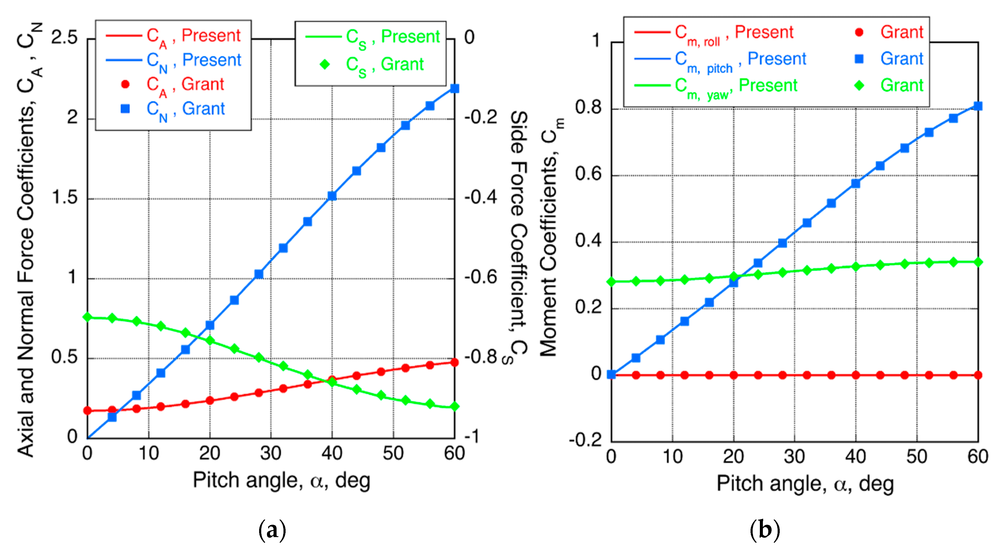
The program code has been further verified for the case that a blunted double-cone is placed in a freestream with angle-of-attack shown in Figure 4. The test case was taken from the work of Grant et al. [10], in which the Newtonian aerodynamic coefficients are calculated by integration using Matlab software. Their results have been verified by comparing them with the results from CBAERO code [11], which employs a panel method.

The pressure coefficient distributions calculated by MC-NEW are shown in Figure 5 for the case of the pitch angle of 10 deg and the yaw angle of 20 deg. In Figure 5, the visible and hidden region in the view from the upstream is clearly divided, and the high-pressure coefficient region appears on the windward side of the nose and the front cone where the normal vector makes small angles with the freestream. The number of visible points was about 13 million, and the computation CPU time was about 2 s.

The calculated axial, normal, and side force coefficients are compared with Grant’s result in Figure 6a, and the rolling, pitching, and yawing moment coefficients in Figure 6b. The variations of coefficients according to the change in the pitching moment in the present results agree well with the Grant’s results.

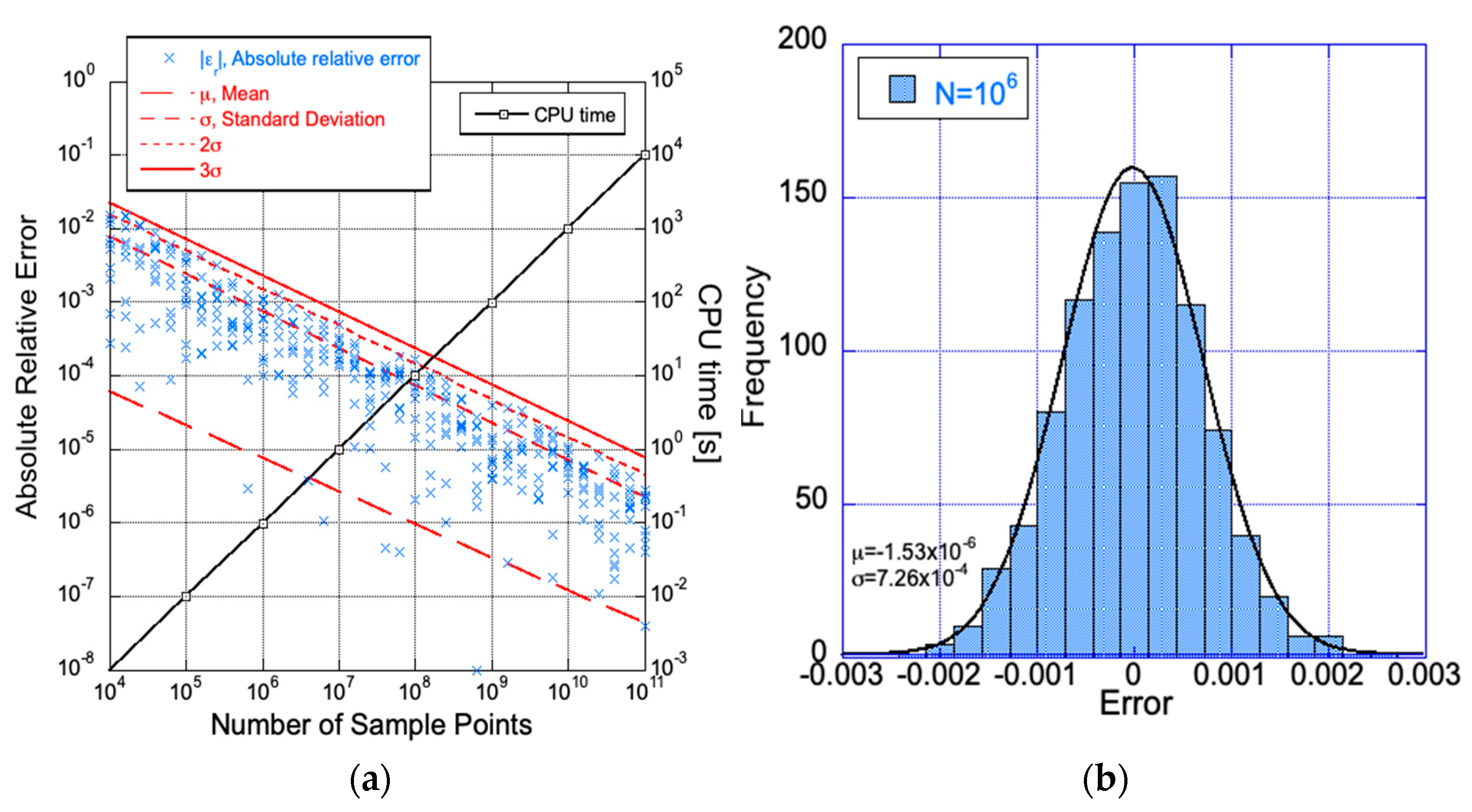
3.3. Accuracy Evaluation

To evaluate the aerodynamic coefficient prediction ability of the MC-NEW program in terms of accuracy, the relation between the prediction error and the total sample point number has been tested. Figure 7a shows the error decreasing history when increasing the sample point number up to 10¹¹, which are obtained from ten trials for predicting the drag coefficient of a hemisphere. Because the Monte Carlo integration is a stochastic method and the errors have deviations, it is difficult to know a clear relationship between the error and the sample point number by several trials. As shown in the frequency histogram of the error over 1000 trials in Figure 7b, the error distribution follows a normal distribution of a black curve. Therefore, the deviations of the error have been evaluated by taking statistics of 1000 trials with the various sample numbers between 10⁴ and 10⁹, and tabulated in Table 2, and their fitting functions are also displayed in Figure 7a. It is generally known that the accuracy of the Monte Carlo integration increases proportionally to the reciprocal of the square root of the sample number. This is the case and the standard deviations in Table 2 are fitted roughly by the following expression;

$$\sigma =\frac{0.8}{\sqrt{N_{\mathrm{visible}}}}.$$

(31)

By taking $3\sigma$ as a possible maximum absolute relative error, the relative error against the analytical solution in the results from MC-NEW program is evaluated by

$$|{ϵ}_{r,\max }|\hspace{0.33em}\le \frac{2.4}{\sqrt{N_{\mathrm{visible}}}},$$

(32)

where $N_{\mathrm{visible}}$ here should be the number of visible sample points that contribute to the summation in Equation (30). According to Equation (32), MC-NEW has the capability to predict the analytical Newtonian aerodynamic coefficients within the ±0.22% error with the probability of 99.7% when one million sample points are used.

The accuracy of the prediction and the computational time are in a trade-off relation. Rough standard computational CPU time as a function of a total number of sample points is also shown in Figure 7a and Table 2, which are measured by using an Intel(R) Xeon(R) Gold 5218R CPU with a clock rate of 2.10 GHz. The computational CPU time proportionally increases with the sample point number. For practical use, sample point numbers from 10⁶ to 10⁸ seem to be a good compromise between the accuracy and the computational time.

Figure 7. Prediction accuracy of the present program for a drag coefficient prediction of a hemisphere: (a) The relation between the total sample point number and the relative error and the computational time; (b) Frequency distribution of error obtained from 1000 trials with 1,000,000 sample points.

Figure 7. Prediction accuracy of the present program for a drag coefficient prediction of a hemisphere: (a) The relation between the total sample point number and the relative error and the computational time; (b) Frequency distribution of error obtained from 1000 trials with 1,000,000 sample points.

Table 2. Relations between total sample point number, parameters for normal distribution of the error, and rough standards of computational CPU time.

Number of	Mean	Diviation			CPU Time 1
Sample Points	μ	σ	2σ	3σ	[s]
104	7.84 × 10−5	7.46 × 10−3	1.49 × 10−2	2.24 × 10−2	0.001
105	5.54 × 10−5	2.47 × 10−3	4.94 × 10−3	7.41 × 10−3	0.01
106	1.53 × 10−6	7.26 × 10−4	1.52 × 10−3	2.18 × 10−3	0.1
107	1.70 × 10−6	2.38 × 10−4	4.76 × 10−4	7.14 × 10−4	1
108	1.56 × 10−6	7.25 × 10−5	1.45 × 10−4	2.90× 10−4	10
109	4.75 × 10−7	2.26 × 10−5	4.52 × 10−5	6.78 × 10−5	100

¹ The CPU time was measured by using a Intel(R) Xeon(R) Gold 5218R CPU@2.10 GHz.

Table 2. Relations between total sample point number, parameters for normal distribution of the error, and rough standards of computational CPU time.

Number of	Mean	Diviation			CPU Time 1
Sample Points	μ	σ	2σ	3σ	[s]
104	7.84 × 10−5	7.46 × 10−3	1.49 × 10−2	2.24 × 10−2	0.001
105	5.54 × 10−5	2.47 × 10−3	4.94 × 10−3	7.41 × 10−3	0.01
106	1.53 × 10−6	7.26 × 10−4	1.52 × 10−3	2.18 × 10−3	0.1
107	1.70 × 10−6	2.38 × 10−4	4.76 × 10−4	7.14 × 10−4	1
108	1.56 × 10−6	7.25 × 10−5	1.45 × 10−4	2.90× 10−4	10
109	4.75 × 10−7	2.26 × 10−5	4.52 × 10−5	6.78 × 10−5	100

¹ The CPU time was measured by using a Intel(R) Xeon(R) Gold 5218R CPU@2.10 GHz.

3.4. Example of Application: A Parametric Study of Nose and Shoulder Radius on Aerodyanmic Performance of Apollo-like Entry Capsule

In order to show an example of the application of MC-NEW code to a conceptual study of a space vehicle, a parametric study to examine the effect of nose and shoulder radius on the aerodynamic performance of an Apollo-like entry capsule is performed. Here, the Newtonian pressure coefficients are modified by multiplying correction factor considering the pressure behind the shock wave [1]

$$\frac{1}{\gamma M^2}\left\{{\left[\frac{{(\gamma +1)}^2{M}^2}{4\gamma M^2-2(\gamma -1)}\right]}^{\gamma /(\gamma -1)}\left[\frac{1-\gamma +2\gamma M^2}{\gamma +1}-1\right]\right\},$$

(33)

where $M$ is the Mach number and $\gamma$ is the specific heat ratio of the freestream.

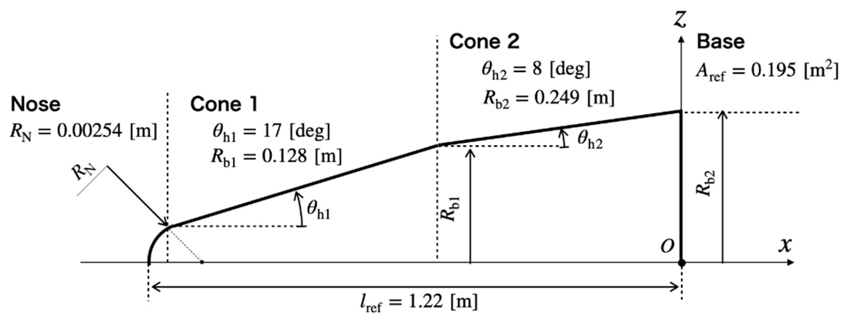
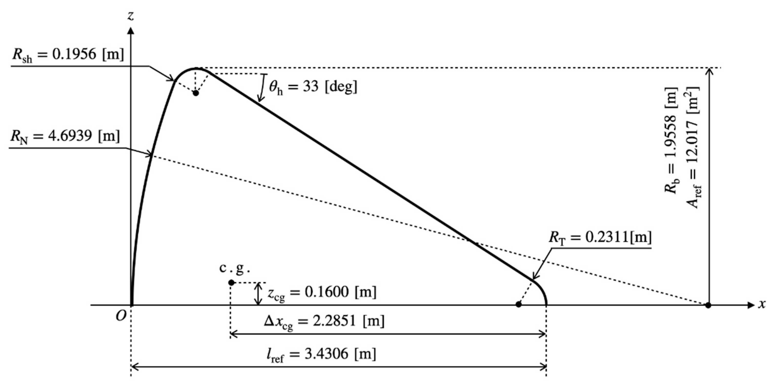
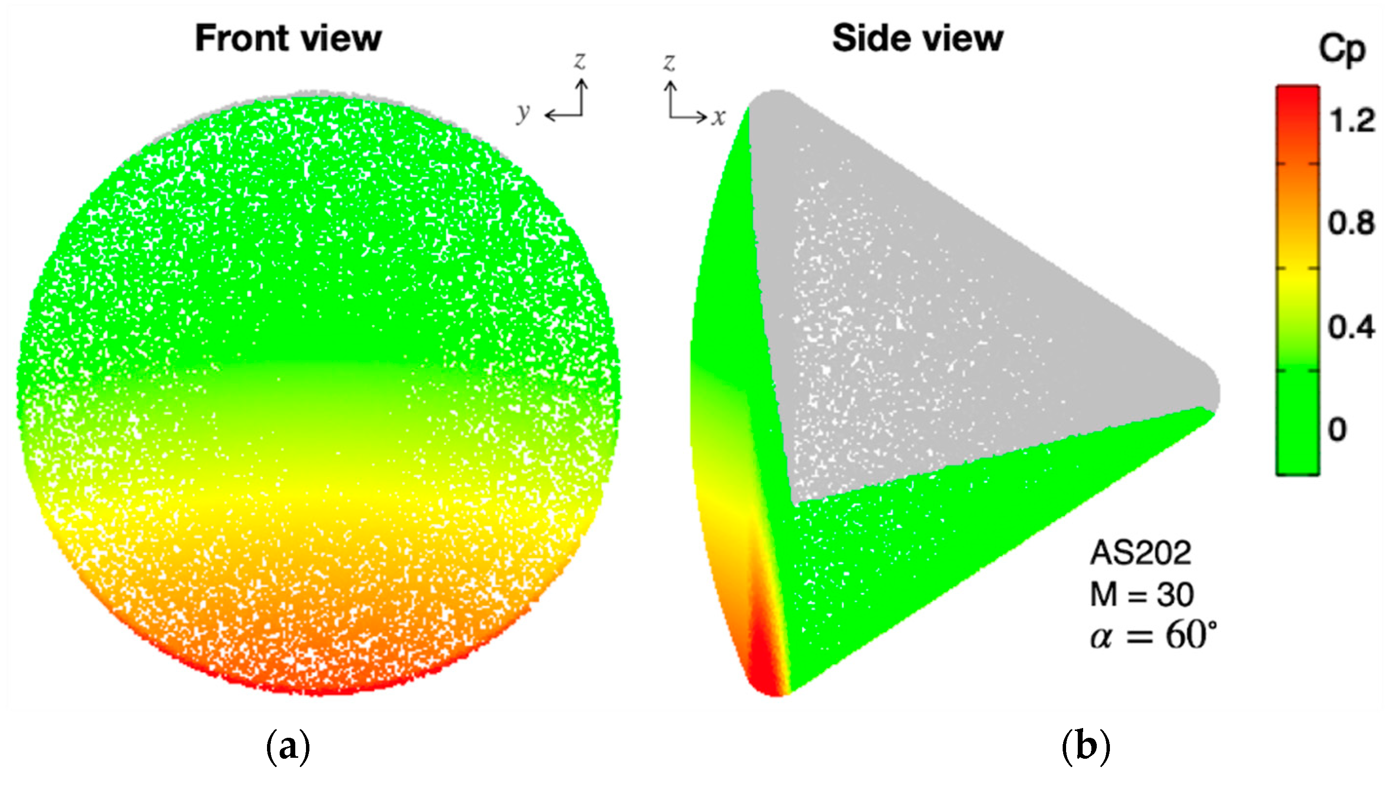
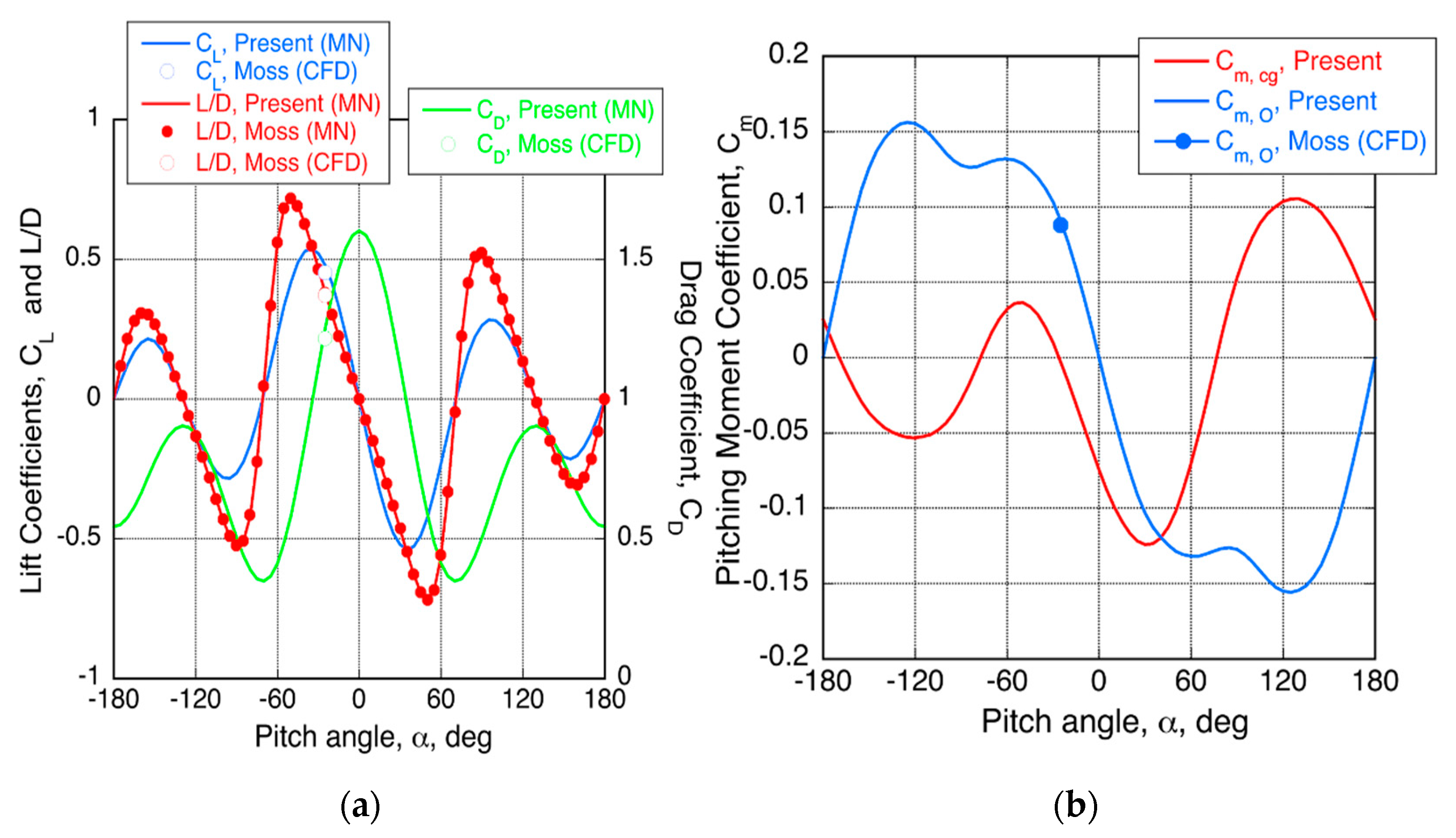
The baseline test case is taken from Moss’s work [12] for the Apollo command module capsule geometry shown in Figure 8. For the flowfield of Mach number of 30, the pressure coefficient distributions calculated by MC-NEW are shown in Figure 9 for the case of the pitch angle-of-attack of 60 deg. As shown in Figure 10, the variation of drag and lift coefficients are the lift-to-drag ratio for the pitch angle-of-attack from −180 to 180 deg, agreeing well with the values in Moss’s work.

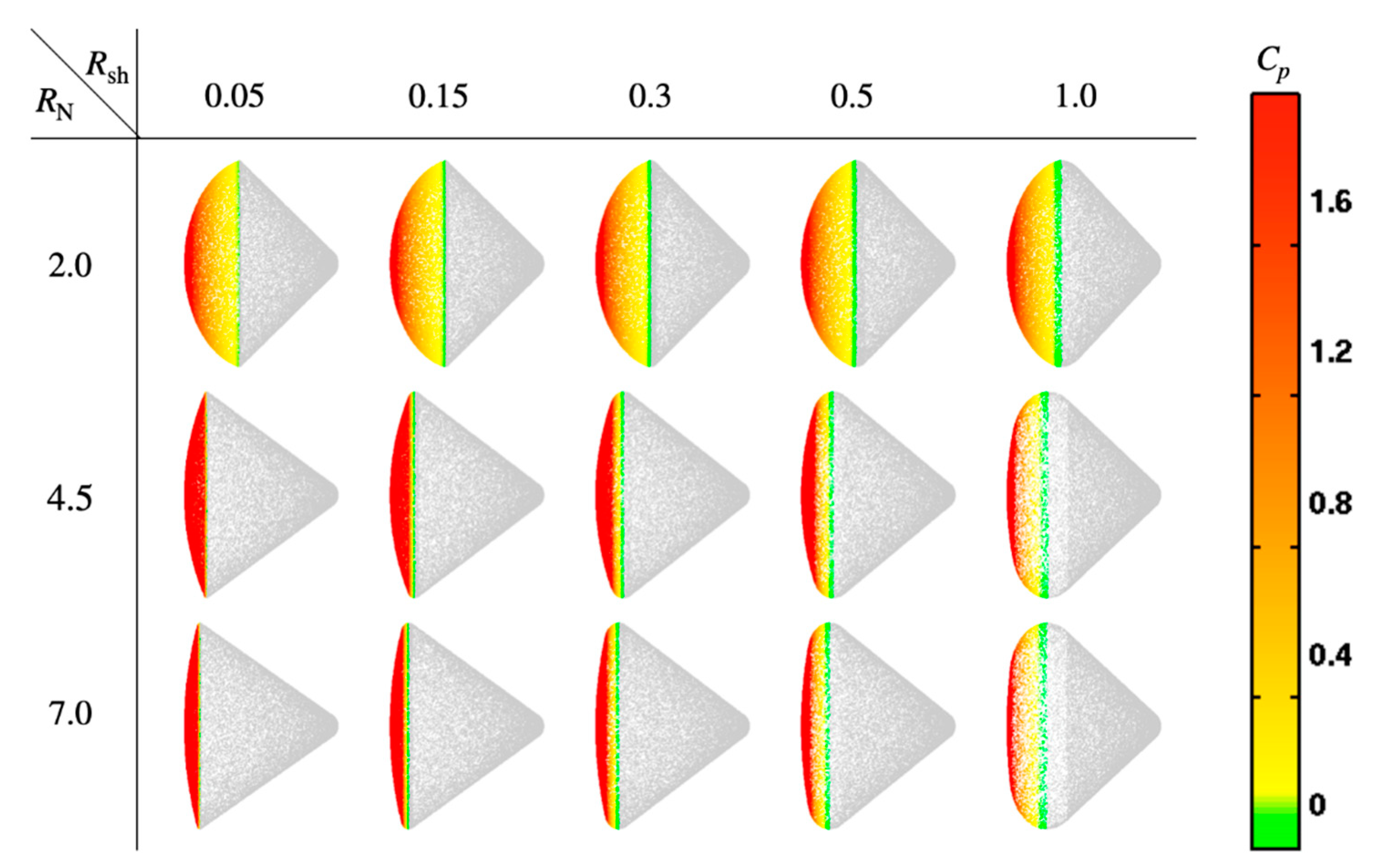
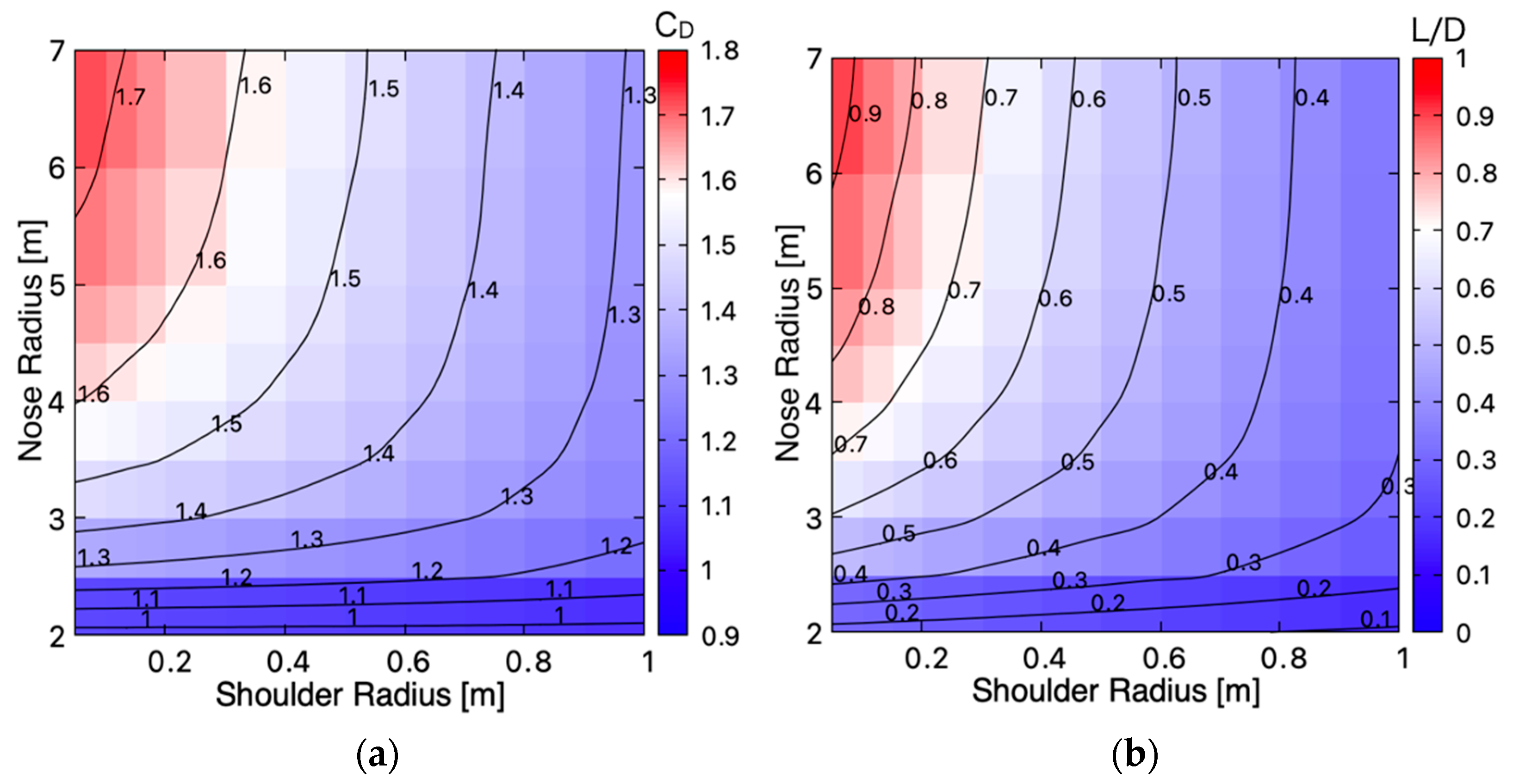
Now, the parametric study is performed by varying the nose and the shoulder radius in the range of 2 < $R_{\mathrm{N}}$ < 7 m and 0.05 < $R_{\mathrm{sh}}$ < 1 m, respectively. The surface local pressure distributions for selected cases are shown in Figure 11. It is shown that the connections between the nose sphere, the shoulder, and the frustum cone are well defined for all the cases. The obtained drag coefficients at 0-degree angle-of-attack and the maximum lift-to-drag ratio are shown in Figure 12 as maps on the nose and the shoulder radius field. It is shown that these aerodynamic coefficients increase as the nose radius increase but decrease as the shoulder radius increases. It is also shown that aerodynamic coefficients are insensitive to the shoulder radius when the nose radius is close to the fixed base radius, $R_{\mathrm{b}}$ < 1.9558 m. 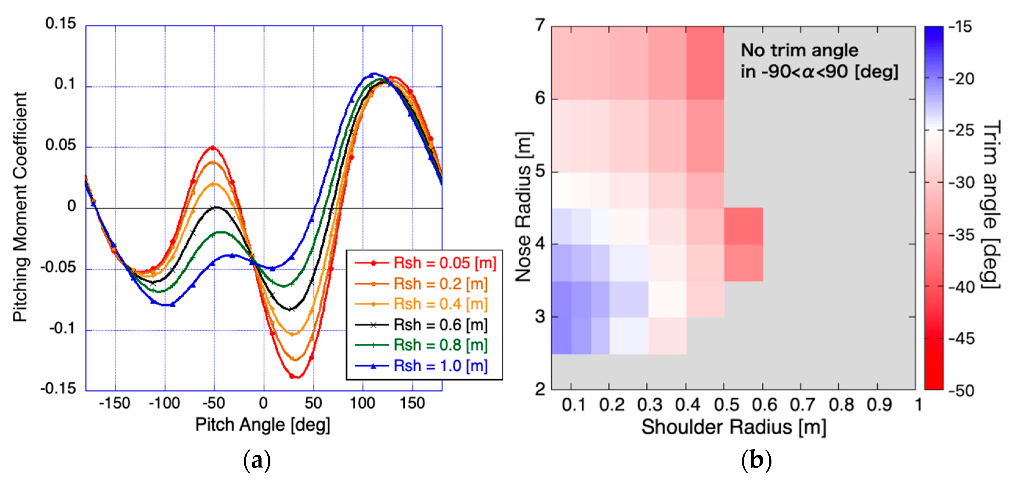Figure 13 shows the variation of the pitching moment about the fixed center of gravity and of the stable trim angle when the nose and the shoulder radius are changed. As seen in Figure 13a, the absolute peak values of the pitching moment as well as the gradient of the moment with respect to the pitch angle decrease when the shoulder radius increase. For the cases with a large shoulder radius, the stable trim angle cannot be found in the range −90 < $\alpha$ < 90 deg, as seen in Figure 13b. It is shown that the absolute value of trim angle increases with the shoulder radius increases and has a minimum value for the nose radius variation.

As shown in this example, one can utilize the present MC-NEW code for the conceptual design of a space vehicle.

4. Discussion

The present Monte-Carlo-based method has the following advantages over the commonly used panel methods. First, users are free from the computational mesh generation. From the input parameters of geometries, such as radius or half-angle, the program calculates intersections between geometries. Therefore, parametric studies on geometries can be performed more efficiently without consuming the time for mesh regeneration. Secondly, the accuracy of the solutions is clear. The accuracy of the Monte-Carlo integration is determined by a function of sample points, and the relation for the present program is given by Equation (32). This program provides good approximations of exact solutions when using enough sample points.

Although the physical accuracy of the Newtonian theory itself can be limited, the program will be useful as a simple tool for designing hypersonic vehicles at the initial design stage, for providing analytical solutions to be a reference for verifications of other codes, and for producing massive data to apply data-science approaches.

Currently, the present program can treat axisymmetric convex surfaces expressed by analytical functions, and the code will be extended for more general geometries in the future.

5. Conclusions

The present study presents a computer program, MC-New, to calculate Newtonian aerodynamic coefficients without generating computational mesh system. The surface geometries of hypersonic vehicles are expressed by a combination of simple geometry given in analytical functions, and the surface integral of the force is evaluated in a Monte-Carlo manner; the force components of randomly distributed sample points are summed-up to calculate aerodynamic coefficients. The developed code was verified against analytical solutions and the results in the past literature. The accuracy analysis in terms of the reproduction of exact solutions unveiled that MC-NEW can predict the analytical Newtonian aerodynamic coefficients within the ±0.22% error with the probability of 99.7% when one million sample points are used. The computation time for a one million sample points calculation is as short as 0.1 s. The presented program can be utilized as a simple tool for designing hypersonic vehicles at the initial design stage as well as for providing reference values for verification of the results by other means. The code will be further improved to have capabilities for more complex geometries in the future. The current version of MC-New is an open-source program released under the MIT license, and the Fortran code can be downloaded as a Supplementary Materials.

References

- Anderson, J.D. Hypersonic and High Temperature Gas Dynamics; McGraw-Hill: New York, NY, USA, 1989. [Google Scholar]
- Weilmuenster, K.J.; Gnoffo, P.A.; Greene, F.A. Navier-Stokes simulations of Orbiter aerodynamic characteristics including pitch trim and bodyflap. J. Spacecr. Rocket. 1994, 31, 355–366. [Google Scholar] [CrossRef]
- Maus, J.R.; Griffith, B.J.; Szema, K.Y.; Best, J.T. Hypersonic Mach Number and Real Gas Effects on Space Shuttle Orbiter Aerodynamics. J. Spacecr. Rocket. 1984, 21, 136–141. [Google Scholar] [CrossRef]
- Heybey, W.H. Newtonian Aerodynamics for General Body Shapes with Several Applications; NASA TM X-53391; The George C. Marshall Space Flight Center (MSFC): Huntsville, AL, USA, 1966. [Google Scholar]
- Clark, E.L.; Trimmer, L.L. Equation and Charts for the Evaluation of the Hypersonic Aerodynamic Characteristics of Lifting Configurations by the Newtonian Theory; AEDC-TDR-64-25; Arnold Engineering Development Center: Tullahoma, TN, USA, 1964. [Google Scholar]
- Bonner, E.; Clever, W.; Dunn, K. Aerodynamics Preliminary Analysis System II Part I Theory; NASA CR-182076; National Aeronautics and Space Administration: Washington, DC, USA, 1991. [Google Scholar]
- Mehta, P.M.; Minisci, E.; Vasile, M.; Walker, A.C.; Brown, M. An Open-Sourse Hypersonic Aerodynamic and Aerothermodynamic Modeling Tool. In Proceedings of the 8th European Symposium on Aerothermodynamics for Space Vehicles, Lisbon, Portugal, 2–6 March 2015. [Google Scholar]
- Aprovitola, A.; Iuspa, L.; Viviani, A. Thermal Protection System Design of a Reusable Launch Vehicle Using Integral Soft Objects. Int. J. Aerosp. Eng. 2019, 2019, 6069528. [Google Scholar] [CrossRef]
- Aprovitola, A.; Iuspa, L.; Pezzella, G.; Viviani, A. Phase-A Design of a Reusable Re-Entry Vehicle. Acta Astronaut. 2021, 187, 141–155. [Google Scholar] [CrossRef]
- Grant, M.; Braun, R. Analytic Hypersonic Aerodynamics for Conceptual Design of Entry Vehicles. In Proceedings of the 48th AIAA Aerospace Sciences Meeting Including the New Horizons Forum and Aerospace Exposition, Orlando, FL, USA, 4–7 January 2010; American Institute of Aeronautics and Astronautics: Reston, VA, USA. [Google Scholar]
- Kinney, D. Aerodynamic Shape Optimization of Hypersonic Vehicles. In Proceedings of the 44th AIAA Aerospace Sciences Meeting and Exhibit, Reno, NV, USA, 9–12 January 2006; American Institute of Aeronautics and Astronautics: Reston, VA, USA. [Google Scholar] [CrossRef]
- Moss, J.; Glass, C.; Greene, F. DSMC Simulations of Apollo Capsule Aerodynamics for Hypersonic Rarefied Conditions. In Proceedings of the 9th AIAA/ASME Joint Thermophysics and Heat Transfer Conference, San Francisco, CA, USA, 5 June 2006; American Institute of Aeronautics and Astronautics: Reston, VA, USA. [Google Scholar]