Flight Anomaly Detection via a Deep Hybrid Model

Abstract

In the civil aviation industry, security risk management has shifted from post-accident investigations and analyses to pre-accident warnings in an attempt to reduce flight risks by identifying currently untracked flight events and their trends and effectively preventing risks before they occur. The use of flight monitoring data for flight anomaly detection is effective in discovering unknown and potential flight incidents. In this paper, we propose a time-feature attention mechanism and construct a deep hybrid model for flight anomaly detection. The hybrid model combines a time-feature attention-based convolutional autoencoder with the HDBSCAN clustering algorithm, where the autoencoder is constructed and trained to extract flight features while the HDBSCAN works as an anomaly detector. Quick access record (QAR) flight data containing information of aircraft landing at Kunming Changshui International and Chengdu Shuangliu International airports are used as the experimental data, and the results show that (1) the time-feature-based convolutional autoencoder proposed in this paper can better extract the flight features and further discover the different landing patterns; (2) in the representation space of the flights, anomalous flight objects are better separated from normal objects to provide a quality database for subsequent anomaly detection; and (3) the discovered flight patterns are consistent with those at the airports, resulting in anomalies that could be interpreted with the corresponding pattern. Moreover, several examples of anomalous flights at each airport are presented to analyze the characteristics of anomalies.

1. Introduction

Flight safety is one of the most important topics in civil aviation. In recent years, safety risk management in civil aviation has shifted from post-accident investigations and analyses to pre-accident warnings. With the expectation of more departing flights in the future, civil aviation aims to effectively prevent potential accidents before they occur and thus to remain at a historically low level of accidents per year. For this, there is a need to innovatively and proactively identify operationally significant safety events that are currently untracked and then implement risk mitigation in the form of revising safety requirements to address the newly identified vulnerabilities. Identifying vulnerabilities or hazards is a key step in the process of risk reduction, for which machine learning can provide assistance [1].

Quick access record (QAR) equipment, installed on aircraft, is equipment used to quickly record various flight parameters during flight. QAR data contain up to 2000 flight parameters, including all kinds of attitude parameters, dynamic parameters, external environment parameters, and flight operation parameters. Each flight parameter is recorded once a second, and some parameters are recorded up to eight times a second. QAR data provide comprehensive information on the status and details of aircraft during flight and can be used for flight safety research and analysis. At the end of 2013, the Civil Aviation Administration of China (CAAC) officially approved the project of the China Civil Aviation Flight Quality Monitoring Base Station and assigned the Civil Aviation Institute of Science and Technology of China (CASTIC) to collect, process and analyze all data recorded by the QAR equipment of all transport aircraft in China. The station achieved the first aggregation of industry-wide flight data at the national level and collected QAR data for more than 3000 aircraft from all 51 transport airlines in China by the end of 2017. Approximately 1500 flight data points are automatically gathered by this station every day, forming a massive and rich QAR flight big dataset, which provides a database and a guarantee for data-driven model research methods. The utilization of QAR data for flight quality monitoring in civil aviation is a scientific approach to ensure flight safety and improve flight efficiency [2].

Identifying flight vulnerabilities could greatly help airline security officers in addressing risks and ensuring flight safety. This can be achieved by precisely detecting anomaly flight records with smart mining techniques and approaches, which helps to mitigate unsafe flight incidents or even accidents that may result in damages to aircraft, injuries, or losses of life. The goal of anomaly detection (also known as outlier detection) is to determine all instances that stand out and are dissimilar to all others in a data-driven fashion [3]. Such instances are known as anomalies and can be caused by errors in the data, but sometimes are indicative of a new, previously unknown, or underlying process. Hawkins [4] defines an outlier as an observation that deviates so significantly from other observations as to arouse suspicion that it was generated by a different mechanism. Therefore, using QAR data for flight anomaly detection is appropriate and effective for identifying situations in which unknown flight risks or security vulnerabilities exist.

In the domain of aerospace, anomaly detection is usually known as exceedance detection, which defines a threshold for specific parameters and detects outliers accordingly. This scenario is largely reliant on empirical studies or expert knowledge, thus limiting its generalizability and usage in detecting complicated flight anomaly incidents. In traditional studies, multiple-kernel-based anomaly detection (MKAD) adopted multiple-kernel learning (MKL) [5,6] to analyze both discrete and continuous sequences, e.g., one-class Support Vector Machines [6,7]. However, MKAD is a semi-supervised method with ground-truth data required, which is very difficult or even unavailable for practical cases. In contrast, cluster-based anomaly detection (ClusterAD) [8] combines the principal component analysis (PCA) and density-based spatial clustering of applications with noise (DBSCAN) techniques to detect flight anomaly. ClusterAD is an unsupervised procedure, and could be more applicable for flight anomaly detections. As noted in [8], however, ClusterAD, is not sensitive to anomalous patterns occurring for short durations. Thus, we tried to develop a new procedure from the ClusterAD for accuracy improvement.

In recent years, deep neural networks have proliferated in the field of machine learning and have achieved unprecedented results across various application domains. As a subset of machine learning, deep learning achieves good performance and flexibility by learning to represent data as a nested hierarchy of concepts within layers of neural networks and outperforms traditional machine learning as the scale of data increases [9]. Therefore, deep learning-based anomaly detection algorithms are increasingly used in various fields and have been proven to be superior to traditional methods [10,11]. Based on the extent of label availability, deep anomaly detection (DAD) can be divided into three categories: (1) supervised DAD; (2) semi-supervised DAD; and (3) unsupervised DAD. Since labeled data are very difficult to obtain in the case of actual tasks, unsupervised DAD algorithms are more widely adopted for anomaly detection tasks because they do not depend on data labels. The unsupervised DAD model and its variants have been shown to outperform traditional methods in many applications [12], such as PCA [13], support vector machine (SVM) [14], and isolation forest [15].

Unsupervised DAD methods can be mainly categorized into three classes: autoencoder (AE)-based, variational AE (VAE)-based and generative adversarial network (GAN)-based methods [16,17,18,19,20,21,22,23].

An AE [24], which mainly contains an encoder and a decoder, is a feed-forward multilayer neural network. It uses an encoder to compress the original data in high-dimensional space into hidden representations in low-dimensional latent space and a decoder to reconstruct the original data from the hidden representations [24]. An AE is trained by minimizing the reconstruction error between its input and its output. Under the assumption that there is a higher prevalence of normal instances than abnormal data instances, AE-based methods use the reconstruction error as an anomaly score. Reddy et al. [16] applied an AE to raw time series data from multiple flight sensors by using sliding overlapping time windows to form input vectors. Zhou et al. [17] implemented an AE with a regularization term (called the “robust AE”) to eliminate outliers in the case of a lack of clean training data.

VAEs [25,26], based on traditional AEs, are a type of deep generative model and have also been extensively used for anomaly detection [18,19,20]. VAEs model high-dimensional distributions by casting learning representations as a variational inference [27] problem. The aim of a VAE is to learn a mechanism that can reveal the probability distribution of the input and generate new samples from random variables that take values in the latent space following the distribution. The optimization process takes into account the quality of autoencoded samples with respect to their reconstruction probability and the Kullback–Leibler (KL) divergence between the prior distribution and the transformed posterior distribution through the encoding process [28]. An anomaly will be reconstructed poorly through the generative process, and its encoding falls outside the distribution.

GANs [29] are another type of generative model that consist of two competing networks, a generator and a discriminator. The generator learns to approximate the distribution of a given dataset, and the discriminator learns to distinguish between real data samples and the generator’s synthetic output samples [29]. GANs have recently been used for anomaly detection [21,22,23,28] and for more advanced variants [30].

Previous studies have achieved good performance and have greatly contributed to our understanding of unsupervised DAD. However, a well-known drawback of neural networks is the lack of interpretability [28]. Moreover, for multi-feature time series data, the inter-time and inter-feature relationships are rarely considered. To avoid these shortcomings in flight anomaly detection, in this paper, we propose a time-feature attention mechanism to capture the inter-time and inter-feature relationships within QAR time series data, and develop an unsupervised deep hybrid model for flight anomaly detection, as shown in Figure 1. Deep hybrid models for anomaly detection use deep neural networks as feature extractors, and the features learned within the hidden representations of autoencoders are input to traditional anomaly detection algorithms [9]. Deep hybrid model in this study combines a time-feature attention-based convolutional AE (TFA-CAE) neural network model with a hierarchical density-based spatial clustering of applications with noise (HDBSCAN) [31] algorithm, where TFA-CAE is built and trained for the extraction of flight features while HDBSCAN employs the extracted flight features to detect anomalous flights. With the size of latent space is set 2, anomalous flights detected with the unsupervised deep hybrid model are more intuitively interpreted and comprehensible.

The remainder of this paper is organized as follows. Section 2 presents the methodology used in our research, and the results of the case study experiment are presented in Section 3. Section 4 contains a summary and conclusion of the paper and an outline of further research.

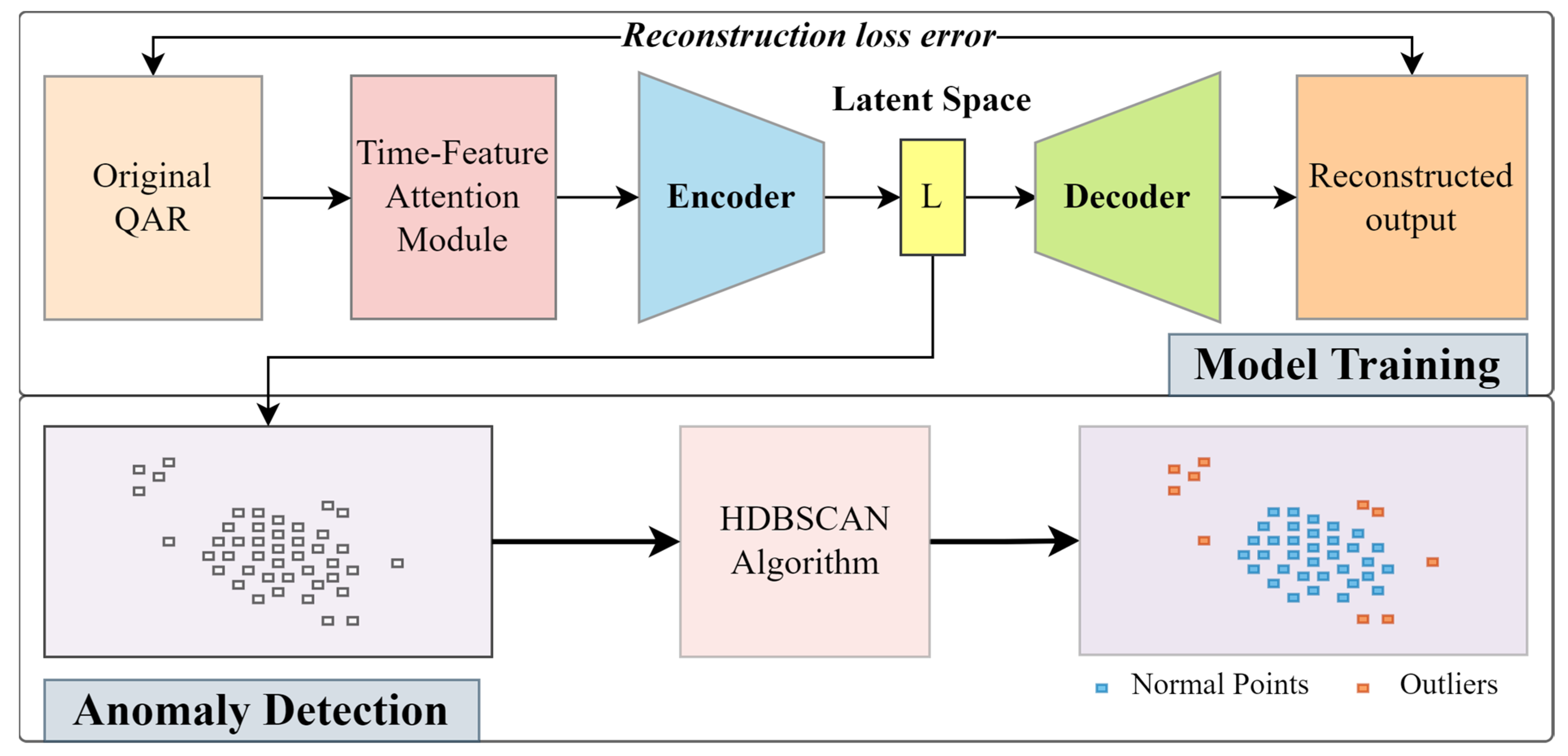
2. Method

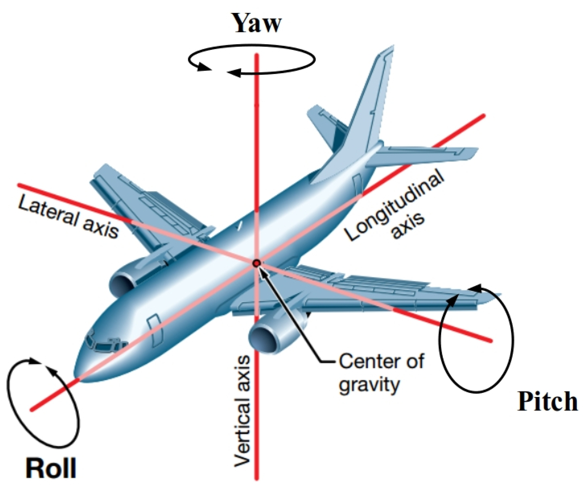
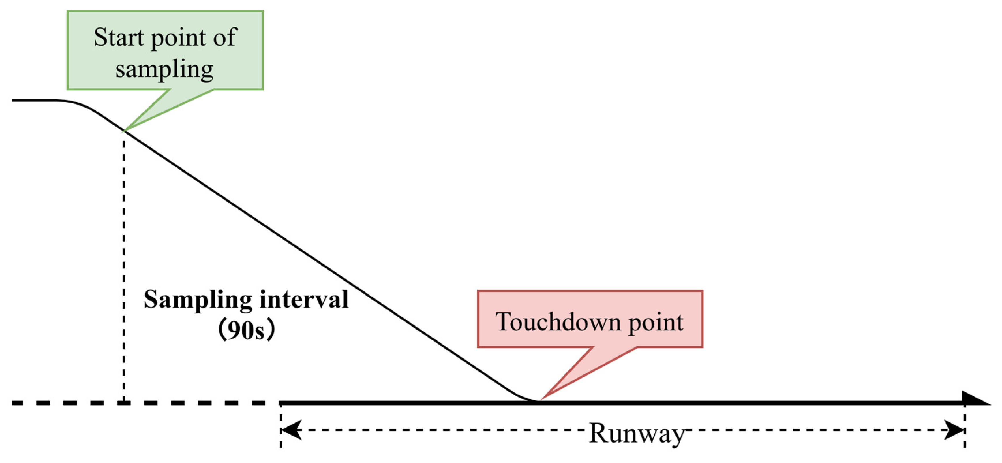
2.1. Data Preprocessing

Generally, aircraft in flight are affected by many factors, such as the external atmospheric environment (wind direction, wind speed, temperature, etc.), the aircraft itself (the position of all control surfaces, engine status, etc.), the pilot’s basic capabilities and skills (cognitive reliability, flight operations skills, etc.), and the pilot’s mental state (fatigue, emotional status, etc.) [32]. During flight, these factors are in constant flux and have a continuous and complex impact on the aircraft. Regardless of how these factors change, however, their effects are ultimately reflected in the change in aircraft attitude and kinematic parameters, including the attitude angle, speed, and acceleration in the three longitudinal, vertical and lateral dimensions [33]. Figure 2 shows a kinematic analysis of a flight. In our research, the above two kinds of flight parameters are selected for the extraction of flight features.

Table 1. The details of the selected flight parameters.

Name	Parameter Name in QAR	Units
Angle of attack	AOA	deg
Angle of pitch	PITCH	deg
Angle of roll	ROLL	deg
Angle of flight path	FPA	deg
Rate of pitch change	PITCH_RATE	deg/s
Indicated air speed of calibration	IASC	knot/s
Ground Speed of calibration	GSC	knot/s
Instantaneous vertical velocity	IVV	g
Lateral acceleration G-Force	LATG	g
Longitudinal acceleration G-force	LONG	g
Vertical acceleration G-force	VRTG	g
Radar altitude of calibration	RALTC	ft

shows the details of the specific parameters.

In this article, we focus on the landing phase of a flight. Compared to the entire profile of a normal flight, this phase of a flight is relatively short but has a high percentage of flight accidents. A review of accident statistics indicates that over 45% of all general aviation accidents occur during the approach and landing phases of a flight [34]. Thus, a fixed duration of 90 s before flight touchdown was chosen as the study flight phase for this paper, as shown in Figure 3. For each flight, every flight parameter in Table 1 is sampled at a fixed interval.

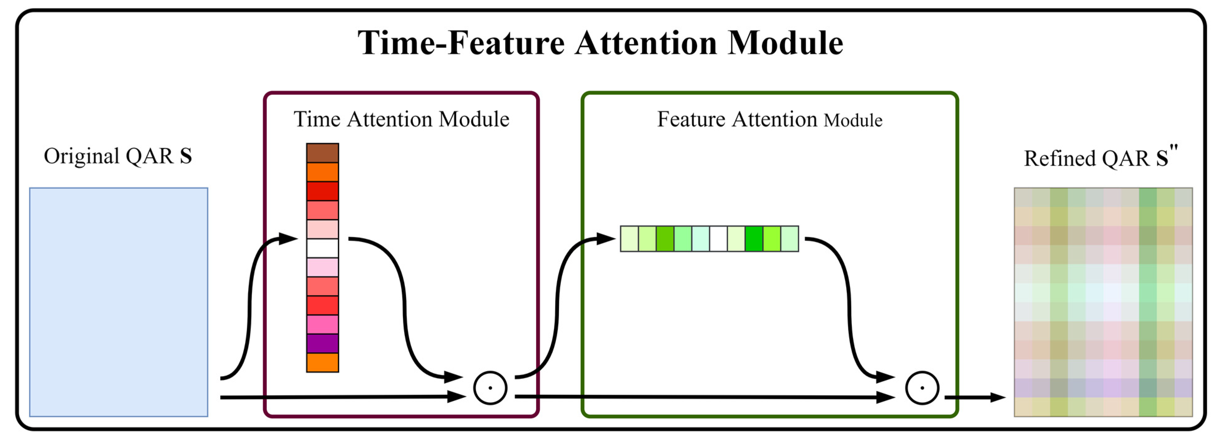
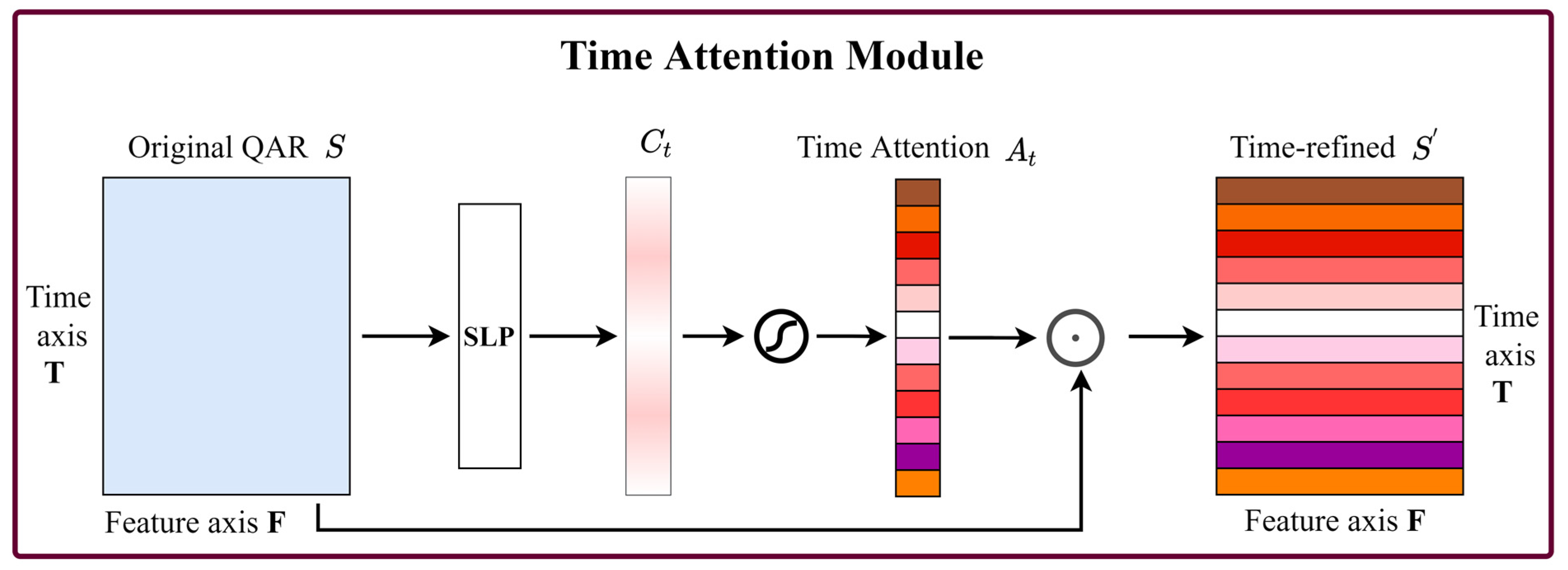
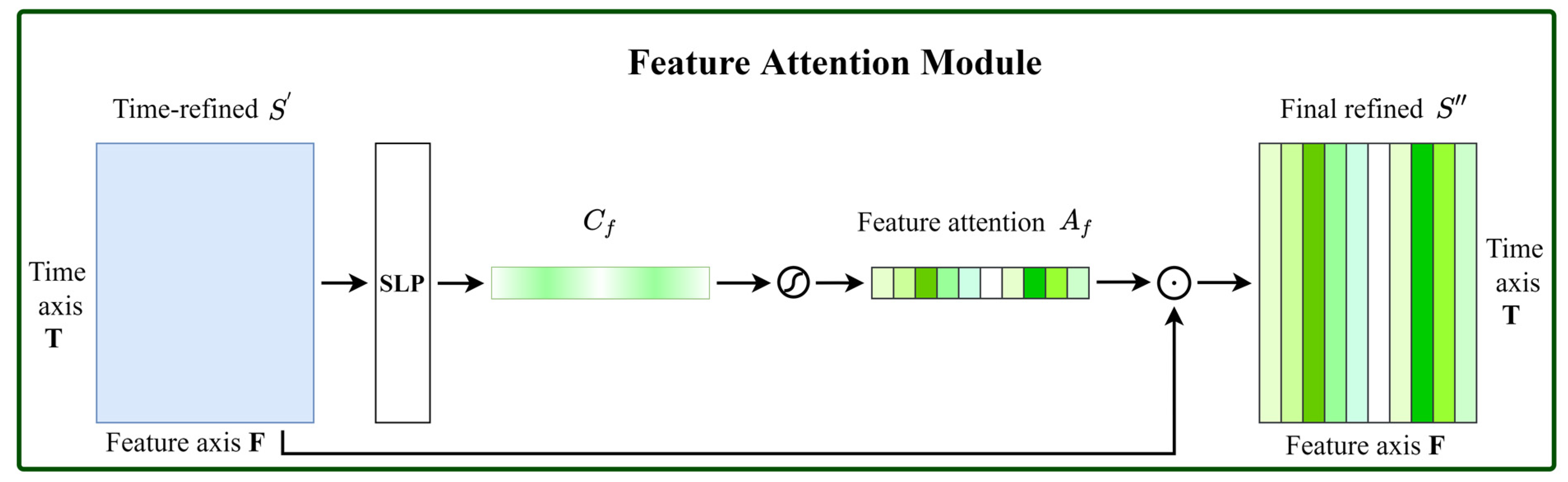
2.2. Time-Feature Attention Module

Previous literature [35,36,37,38,39,40,41,42] has extensively shown the significance of attention. Attention not only tells where to focus but also improves the representation of interests [42]. As during a certain period, the deviations of anomalous flights occur to one or more features, our goal is to know when (the time of deviation occurs) and which (the features with deviation) to focus on and improve the corresponding values by using an attention mechanism. Thus, we propose a new network module, named the “Time-Feature Attention Module (TFAM)”. To emphasize meaningful features along the time and feature axes, a time module and a feature module are sequentially applied (as shown in Figure 4) so that TFAM can learn “when” and “which” to attend to on the time and feature axes, respectively. As the output of the TFAM module, anomalous flights will be differentiated from the common flights; meanwhile, flights within the same common flight pattern will be more tightly aggregated and apparently separated from the ones within other common patterns.

Given a QAR sequence $\mathit{S}\in {ℝ}^{F\times T}$ as input, where $F$ means the size of feature dimension and $T$ denotes the size of time dimension, the time attention module first infers a 1D time attention map ${\mathit{A}}_{\mathit{t}} \in {ℝ}^{1\times T}$ and produces the time-refined output ${\mathit{S}}^{\prime }\in {ℝ}^{F\times T}$. Afterward, the feature attention module takes ${\mathit{S}}^{\prime }\in {ℝ}^{F\times T}$ as input to infer a 1D feature attention map ${\mathit{A}}_{\mathit{f}}\in {ℝ}^{F\times 1}$ and generates the final refined output ${\mathit{S}}^{″}\in {ℝ}^{F\times T}$. The computation process of overall attention can be summarized as follows:

$$\begin{gathered} {\mathit{S}}^{\prime }={\mathit{A}}_{\mathit{t}}\left(\mathit{S}\right) \odot \mathit{S} \\ {\mathit{S}}^{″}={\mathit{A}}_{\mathit{f}}\left({\mathit{S}}^{\prime }\right)\odot {\mathit{S}}^{\prime } \end{gathered}$$

(1)

where $\odot$ denotes the Hadamard product operation. In performing the multiplication operation, the time attention values are propagated (copied) along the dimension of the feature parameters, and the feature attention values are propagated along the time dimension. Figure 5 and Figure 6 depict the computation processes of the time attention and feature attention modules, respectively.

Time Attention Module. The role of the time attention mechanism is to give more attention to the key flight time. A time attention map is produced by exploiting the inter-time relationship of QAR time series data, and each time of a sample works as a time detector, as shown in Figure 5. To efficiently compute the time attention, we squeeze the feature dimension of the input QAR time series. Given a QAR time series $\mathit{S} \in {ℝ}^{F\times T}$ as input, the feature information of $\mathit{S} \in {ℝ}^{F\times T}$ is first aggregated by using a single-layer perception (SLP) along the time axis to generate a context descriptor of the feature parameters ${\mathit{C}}_{\mathit{t}}$. To produce the time attention map ${\mathit{A}}_{\mathit{t}}\left(\mathit{S}\right) \in {ℝ}^{1\times T}$, a sigmoid function is applied to the context descriptor ${\mathit{C}}_{\mathit{t}}$. Finally, we multiply time attention ${\mathit{A}}_{\mathit{t}}\left(\mathit{S}\right)\in {ℝ}^{1\times T}$ and $\mathit{S} \in {ℝ}^{F\times T}$ by the Hadamard product to obtain the time-refined ${\mathit{S}}^{\prime }\in {ℝ}^{F\times T}$. The time attention ${\mathit{A}}_{\mathit{t}}\left(\mathit{S}\right)\in {ℝ}^{1\times T}$ and time-refined ${\mathit{S}}^{\prime }\in {ℝ}^{F\times T}$ are computed as

$${\mathit{A}}_{\mathit{t}}\left(\mathit{S}\right)=\mathbf{\sigma }({\mathit{W}}_{\mathit{t}}\times \mathit{S})$$

(2)

$${\mathit{S}}^{\prime }={\mathit{A}}_{\mathit{t}}\left(\mathit{S}\right) \odot \mathit{S}$$

(3)

where $\sigma$ denotes the sigmoid function, and $\odot$ denotes the Hadamard product operation. ${\mathit{W}}_{\mathit{t}} \in {ℝ}^{1\times F}$.

Feature Attention Module. Different from time attention, feature attention pays more attention to key features and is complementary to time attention. We produce a feature attention map by probing the inter-feature relationship of a QAR time series. The computation of feature attention is very close to the computation process of time attention except that we squeeze the time dimension of the time-refined sequence, as shown in Figure 6. First, a single layer perception (SLP) is used to aggregate the temporal information of the time-refined ${\mathit{S}}^{\prime }\in {ℝ}^{F\times T}$ along the feature axis to generate a temporal context descriptor ${\mathit{C}}_{\mathit{f}}$. A feature attention map ${\mathit{A}}_{\mathit{f}}\left({\mathit{S}}^{\prime }\right)\in {ℝ}^{F\times 1}$ is produced after ${\mathit{C}}_{\mathit{f}}$ is forwarded to a sigmoid function. To obtain the final refined output ${\mathit{S}}^{″}\in {ℝ}^{F\times T}$, we multiply ${\mathit{A}}_{\mathit{f}}\left({\mathit{S}}^{\prime }\right)\in {ℝ}^{F\times 1}$ and ${\mathit{S}}^{\prime }\in {ℝ}^{F\times T}$ by the Hadamard product. In short, the feature attention ${\mathit{A}}_{\mathit{f}}\left({\mathit{S}}^{\prime }\right)\in {ℝ}^{F\times 1}$ and ${\mathit{S}}^{″}\in {ℝ}^{F\times T}$ are computed as

$${\mathit{A}}_{\mathit{f}}\left({\mathit{S}}^{\prime }\right)=\mathbf{\sigma }({\mathit{W}}_{\mathit{f}}\times {\mathit{S}}^{{\prime }^{\mathit{T}}})$$

(4)

$${\mathit{S}}^{″}={\mathit{A}}_{\mathit{f}}\left({\mathit{S}}^{\prime }\right) \odot {\mathit{S}}^{\prime }$$

(5)

where $\sigma$ denotes the sigmoid function, and $\odot$ denotes the Hadamard product operation. ${\mathit{W}}_{\mathit{f}} \in {ℝ}^{1\times T}$, and ${\mathit{S}}^{{\prime }^{\mathit{T}}}$ is the matrix transpose of ${\mathit{S}}^{\prime }$.

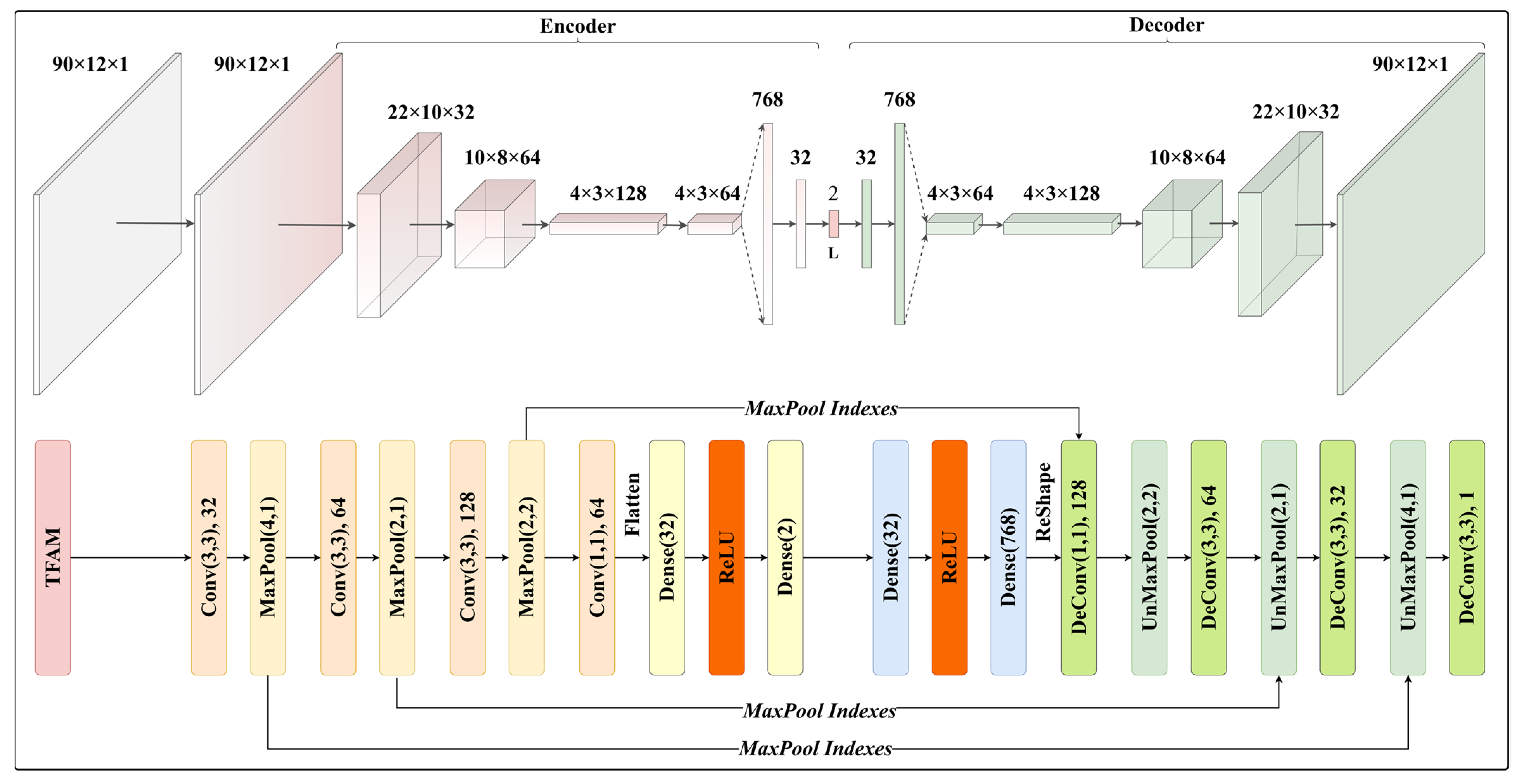
2.3. Time-Feature Attention-Based Convolutional Autoencoder (TFA-CAE)

An AE network is a powerful nonlinear model structure for data reduction and feature extraction. For feature extraction, the AE is built and trained with the goal of representing meaningful attributes of the original data input with the latent space representation as much as possible. Once training is completed, the encoder part can be used as a powerful automatic feature extractor. The architecture of the AE network model, such as convolutional neural network AEs (CNN-AEs) and recurrent neural network AEs (RNN-AEs), is flexible and diverse, and its choice is dependent on the nature of the data. Previously, RNN-based models were considered and preferred for sequential data. However, recent studies have shown that CNN-based models perform better than general RNN-based models [43]. The main advantage of CNNs is their ability to extract complicated hidden features from high-dimensional data with complex structures [44], and they can also be adopted to extract features from sequential data.

In this paper, we construct a TFA-CAE network model for feature extraction of flight data. Figure 7 shows the structure and parameters of TFA-CAE, in which the TFAM is placed in front of the AE. An original QAR time series is first passed through the time-feature module to generate a refined time series. Within the encoder, multi-convolutional and max-pooled layers are stacked on the refined time series to extract hierarchical features, and all units in the last convolutional layer are then flattened to form a vector followed by two fully connected layers, which are called embedded layers. As the second fully connected layer has two units, the input QAR time series is thus transformed into a two-dimensional feature space (latent space). Designed as a symmetrical form, the decoder then reconstructs the original QAR sequence using the features in the latent space.

In the training of TFA-CAE, indexes of each max-pooling layer within the encoder are fed into the symmetrical unmax-pooling layers of the decoder. The error between the original QAR input and the reconstructed output is backpropagated to optimize the parameters of the model. Because our model is trained under the assumption that a small amount of anomalous data exists in the dataset, we use the Huber loss function [45], which is less sensitive to anomalies, to reduce the distortion of the model by anomalous flights.

2.4. HDBSCAN

Clustering is considered to play a significant role in unsupervised learning and deals with the data structure partition in unknown areas. In data science, clustering is used to find patterns or groupings in large datasets and is a general technique with broad applicability across scientific domains. For anomaly detection, objects deviating from patterns or far away from groupings are considered anomalies. As a classic density-based algorithm, density-based spatial clustering of applications with noise (DBSCAN) [46] defines the density at which the number of objects within a neighborhood of a certain radius must reach the specified size (minPts). The size of the radius is specified by the distance threshold parameter $ϵ$ (epsilon). All objects within the connected subsets that fulfill this density threshold are regarded as clusters, while the others are discarded as outliers. This method can detect clusters of different shapes and does not need to specify the number of clusters in advance. However, the major weakness of DBSCAN is that its epsilon parameter serves as a globe density threshold and, therefore, it cannot discover clusters of variable densities [47]. To overcome this problem, many variations of DBSCAN, such as HDBSCAN [31], OPTICS [48], AUTO-HDS [49], and DECODE [50], have been proposed. HDBSCAN has been shown to outperform both AUTO-HDS and the combination of OPTICS with Sander et al.’s [51] cluster extraction method [52]. The main implementation steps of HDBSCAN are shown as follows [53]:

(1)

Transform the space. In the HDBSCAN algorithm, a new distance metric between points called the mutual reachability distance is first defined to spread apart points with low densities:

$$d_{mreach-k}\left(x_p,x_q\right)=max\left\{cor{e}_k\left(x_p\right),cor{e}_k\left(x_q\right),d\left(x_p,x_q\right)\right\}$$

(6)

where $d_{mreach-k}\left(x_p,x_q\right)$ is the mutual reachability distance; $cor{e}_k\left(x_p\right)$ and $cor{e}_k\left(x_q\right)$ are the core distances defined for parameter $k$ for points $x_p$ and $x_q$, respectively; and $d\left(x_p,x_q\right)$ is the original metric distance between $x_p$ and $x_q$. With this metric, points with high density maintain the same distance from each other, while the sparse points are separated from other points by at least their core distance.

(2)

Build the minimum spanning tree. The dataset is then represented by a mutual reachability graph with the data points as vertices and a weighted edge between any two points with weights equal to the mutual reachability distances of those points. A minimum spanning tree of the graph, in which all the weights of all edges are the smallest, is constructed so that removing any edges of the tree will split the graph. The minimum spanning tree can be built quickly and efficiently with Prim’s algorithm [54].

(3)

Build the cluster hierarchy. Given the above minimum spanning tree, the next step is to convert it into a hierarchy of connected components. This is most easily done in the reverse order: sort the edges of the tree by the distances in increasing order and then iterate through them, creating a new merged cluster for each edge. The key here is to identify the two clusters for each edge to join together, which is easily achieved with a union-find data structure [55].

(4)

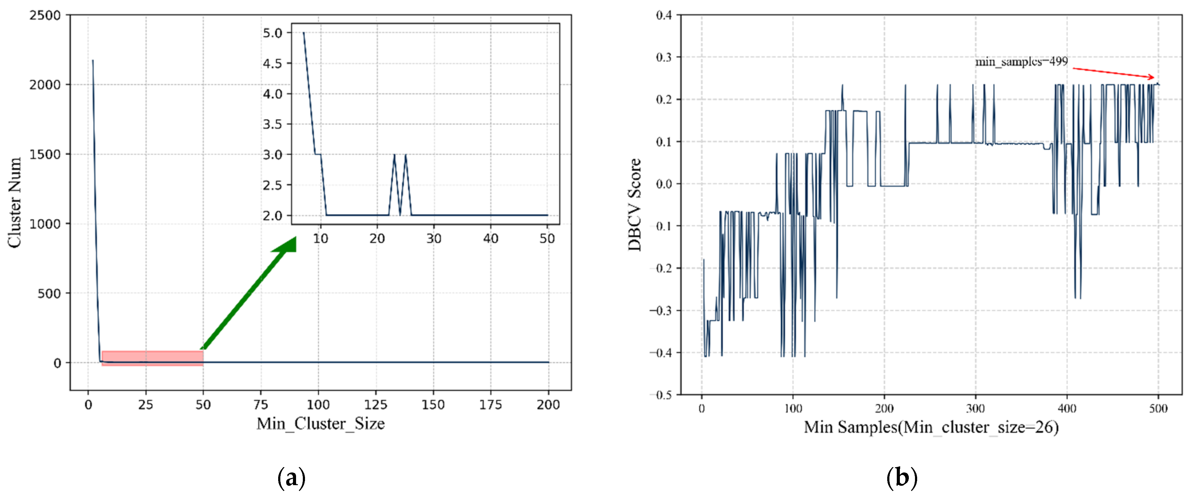
Condense the cluster tree. This step condenses down the large and complicated cluster hierarchy into a smaller tree with slightly more data attached to each node. As the most important parameter of HDBSCAN, min_cluster_size is needed to make this concrete. Starting from the root, when each cluster is split, the samples of subclusters with sizes less than min_cluster_size are detected and marked as “outliers”. If all the subclusters contain fewer than min_cluster_size objects, the cluster is considered to have disappeared at this density level. After walking through the whole hierarchy and completing this process, a tree with a small number of nodes, the condensed cluster tree, is obtained.

(5)

Extract the clusters. HDBSCAN uses $\lambda /distance$ to measure the persistence of clusters and introduces the stability indicator. For each cluster, the stability is computed as:

$$s_{cluster}={{\displaystyle \sum }}_{p\in cluster}\left({\lambda }_p-{\lambda }_{birth}\right)$$

(7)

• ${\lambda }_{birth}:$ the lambda value when the cluster is formed;
• ${\lambda }_{death}:$ the lambda value when the cluster is split into two subclusters;
• ${\lambda }_p:$ the lambda value when point $p$ falls out of the cluster.

where ${\lambda }_{birth}<{\lambda }_p<{\lambda }_{death}$ and $s_{cluster}$ is the stability of the cluster. As a solution to cluster extraction, HDBSCAN’s selection algorithm traverses the condensed cluster tree from bottom to top and selects the cluster with the highest stability on each path.

The HDBSCAN class has a large number of parameters that can be set during initialization, but in practice, few parameters have a significant practical impact on clustering. min_cluster_size (the minimum size of clusters) and min_samples (the number of samples in a neighborhood for a point to be considered a core point) are the two main parameters that affect the anomaly detection results. Increasing min_cluster_size will reduce the number of clusters. The larger min_samples is, the more points there are that are considered outliers, and clusters will be restricted to denser areas.

3. Experimental Result

3.1. Experimental Data

Flight landing data from Kunming Changshui International Airport (ICAO: ZPPP, hereafter) and Chengdu Shuangliu International Airport (ICAO: ZUUU, hereafter) in 2018 are taken as our experimental data in this paper. The dataset contains 14,195 flights, and the data are extracted as described in Section 2.2 and standardized by min-max normalization after the absolute operation for negative parameters. We split the dataset into a training set and a validation set. The training dataset is used to train the model, while the validation dataset is used to determine when to stop the training of the model. The details of the two datasets are shown in

Table 2. The details of the two datasets.

Name of Dataset	Size of Dataset
Training set	9936
Validation set	4259

.

3.2. Model Training

In the experiment of this article, a GRU-based AE (GRU-AE) and a self-attention-based [52] convolutional AE (SA-CAE) are also constructed for comparison with the TFA-CAE. All the models are built and trained using the PyTorch deep learning framework version 1.10. In the network training, early stopping is simultaneously adopted with the patience set to 15, which means model training stops when the loss error of the validation set no longer decreases after 15 epochs. In addition, the “Adam” optimizer is also used to build both models.

Table 3. Comparison of the loss values of TFA-CAE, SA-CAE and GRU-AE.

Models	Loss Errors
TFA-CAE	0.0009
SA-CAE	0.0013
GRU-AE	0.0016

shows the comparison of the average loss values of the models. Because the decoder reconstructs the original QAR time series with the latent space representation mapped by the encoder, a smaller loss error between the original QAR input and the reconstructed outputs indicates a better feature representation of the input. Therefore, TFA-CAE is able to extract more representative features of the flight due to its smaller average loss error, as demonstrated in Table 3.

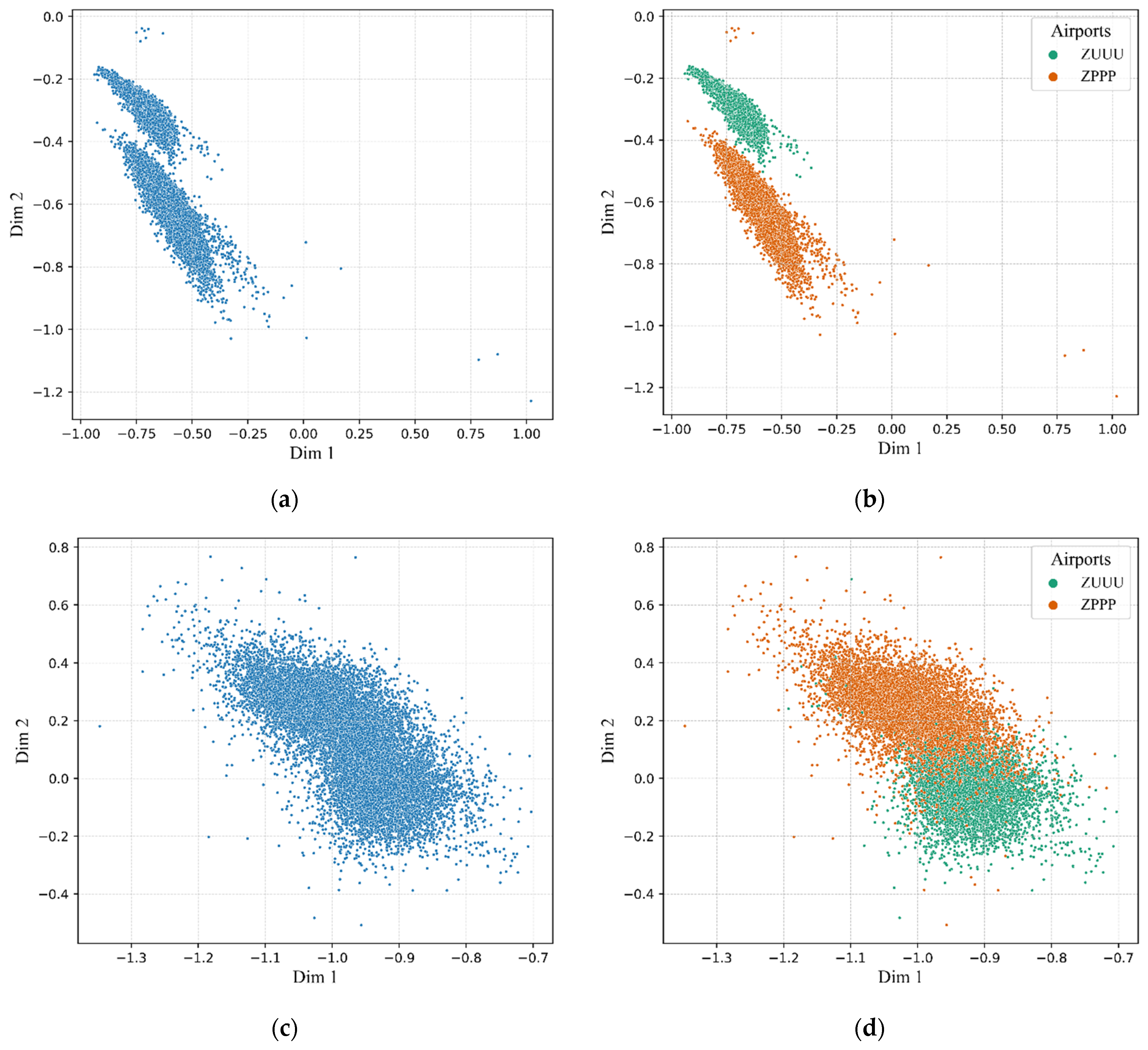
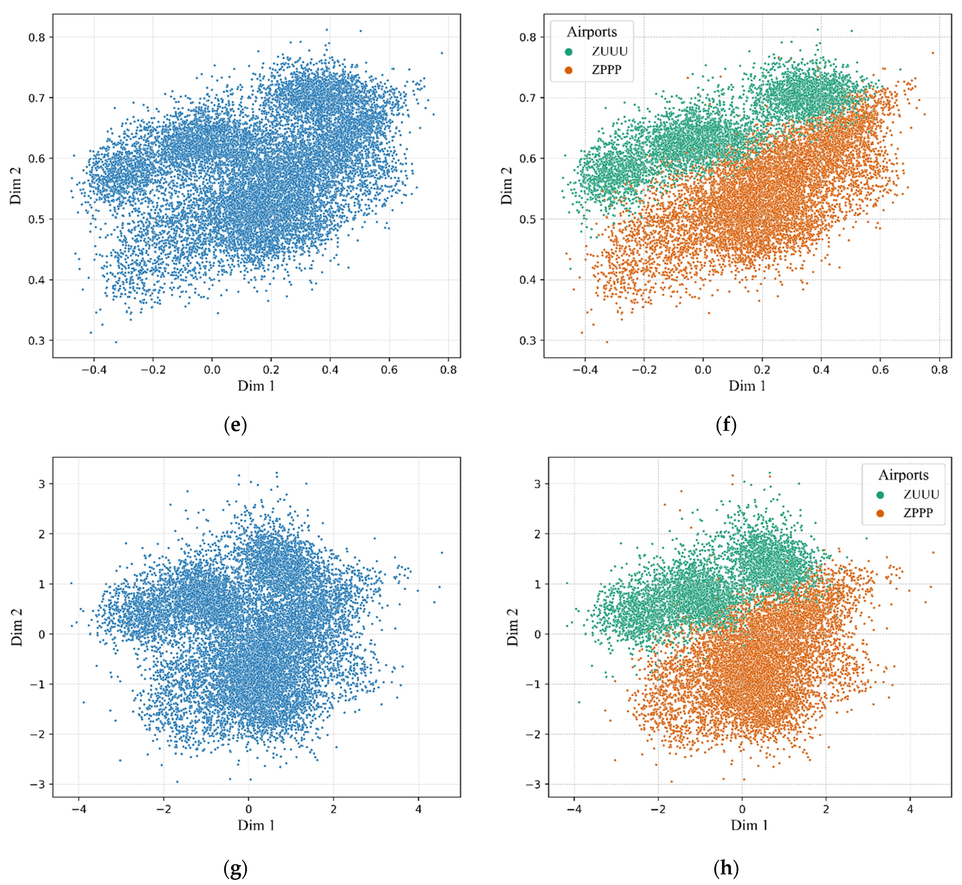
3.3. Visualization of the Extracted Flight Features

As the size of the latent representation is set to two, we are able to visualize the data of the extracted flight features. Figure 8 shows the visualization results of the flight features extracted by each model separately, as well as the PCA. By comparison, the flight features extracted by TFA-CAE are divided into two clusters (shown in Figure 8a), while the others show an irregular pattern of distribution (shown in Figure 8c,e,g). Flight feature objects extracted by TFA-CAE in the same cluster are more tightly aggregated together, while the two clusters are more clearly separated. Considering the fact that an aircraft landing at different airports follows the specific landing procedure for each airport, these two clusters are supposed to indicate the two kinds of landing patterns of the ZPPP and ZUUU airports. To verify the two landing patterns, we further divide the extracted flight features by these two airports separately. The division results of the flight features extracted by each model are separately shown in Figure 8b,d,f,h. In Figure 8b, the two clusters of flight features extracted by the TFA-CAE are consistent with the division according to the airports. For the other division results, the features of these two categories show an intertwined distribution. Based on the above, we summarize that the TFA-CAE model is able to more accurately extract features of flight and further discover different flight patterns, which provides a better feature basis for anomaly detection and analyses of anomalous characteristics.

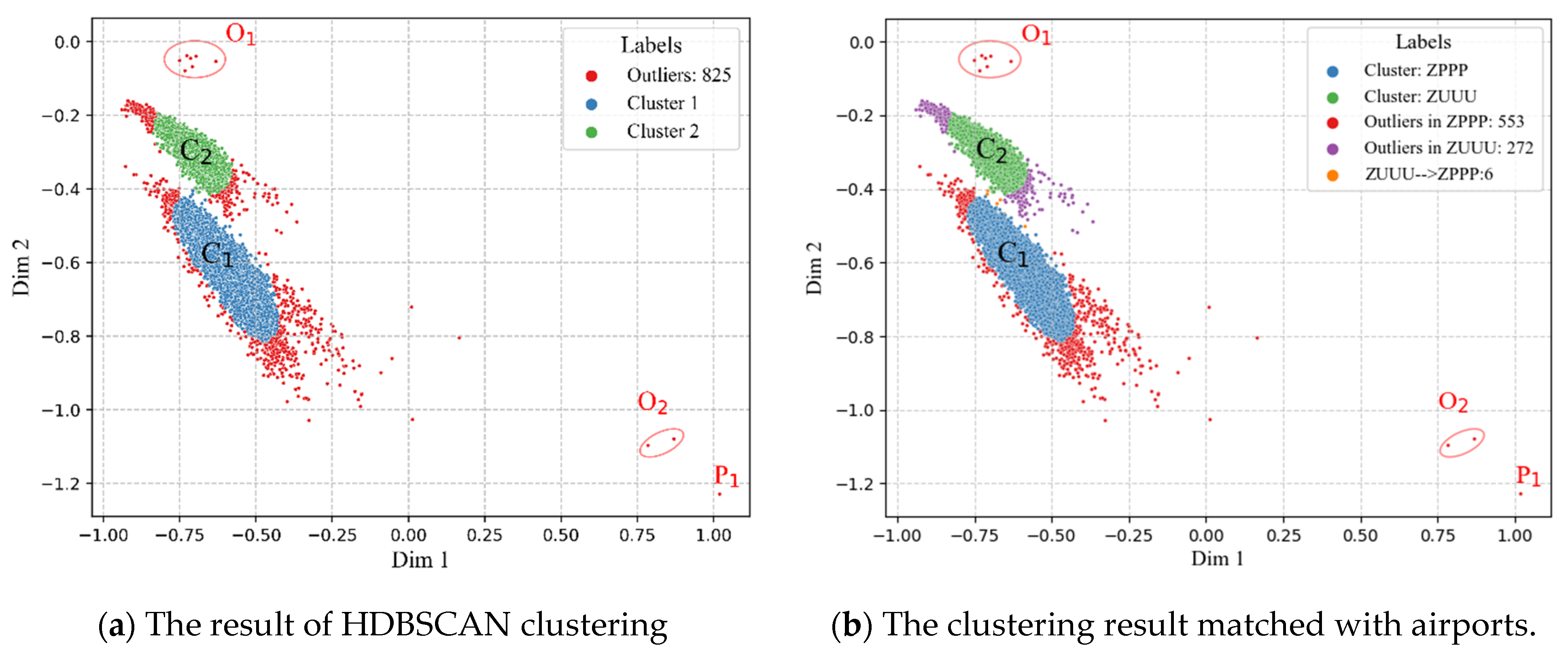
3.4. Result of HDBSCAN Clustering

Flight features extracted by TFA-CAE are fed into the HBSCAN cluster algorithm for flight anomaly detection. From Section 2.4, we know that the input parameters of HDBSCAN are min_cluster_size and min_samples. Therefore, the two parameters are used to determine the results of clustering and need to be specified artificially. To ensure the objectivity of clustering by minimizing manual intervention, we introduce a quantitative measure called the density-based clustering validation (DBCV) index [56] to evaluate and then determine the final clustering result. The index assesses the clustering quality based on the relative density connection between pairs of objects and is formulated on the basis of a new kernel density function, which is used to compute the density of objects and to evaluate the within- and between-cluster density connectedness of the clustering results [57]. Unlike other metrics, such as the silhouette coefficient (SC) [58] and the Davies–Bouldin index (DBI) [59], DBCV takes noise into account and captures the shape property of clusters via densities but not distances and works for density-based clustering algorithms precisely. As explained in their paper, DBCV produces a score between −1 and 1, with the larger the value indicating a better clustering solution.

The optimization goal of HDBSCAN is to find the optimal min_cluster_size and min_samples values that yield the maximum DBCV score. Figure 9 illustrates the process of selecting these two parameters. To avoid a loss of generality, we first fixed min_samples to the default setting and iterated min_cluster_size from 2 to 200 while calculating the number of clusters, as shown in Figure 9a. The number of clusters remained at 2 when min_cluster_size was 26 or greater. Then, we fixed min_cluster_size = 26 and iterated min_samples from 2 to 500 to obtain the maximum DBCV score, as shown in Figure 9b. Finally, we chose min_cluster_size = 26 and min_samples = 499 for our case study.

The result of HDBSCAN clustering of flight features is shown in Figure 10a, in which the red points indicate outliers, while the blue and green points represent two clusters, ${\mathit{C}}_{\mathbf{1}}$ and ${\mathit{C}}_{\mathbf{2}}$, respectively. In the case study, a total of 825 outliers were detected. Furthermore, we matched the clustering result of the extracted flight features with the two airports, as shown in Figure 10b. In detail, ${\mathit{C}}_{\mathbf{1}}$ is a cluster of flights that represents the common landing pattern of the ZPPP airport, while ${\mathit{C}}_{\mathbf{2}}$ represents the landing pattern of the ZUUU airport. A total of 553 anomalous flights (red points) landed at the ZPPP airport, and 272 anomalous flights (purple points) landed at the ZUUU airport. $O_1$ and $O_2$ are two aggregations of anomalous flights that deviate far from the landing pattern of the ZPPP airport; in each cluster, the flights have similar anomalous characteristics. The point $P_1$ represents a flight with the farthest deviation from the common pattern of the ZPPP airport. One drawback is that six flights (orange points) at the ZUUU airport are clustered into the pattern of the ZPPP airport.

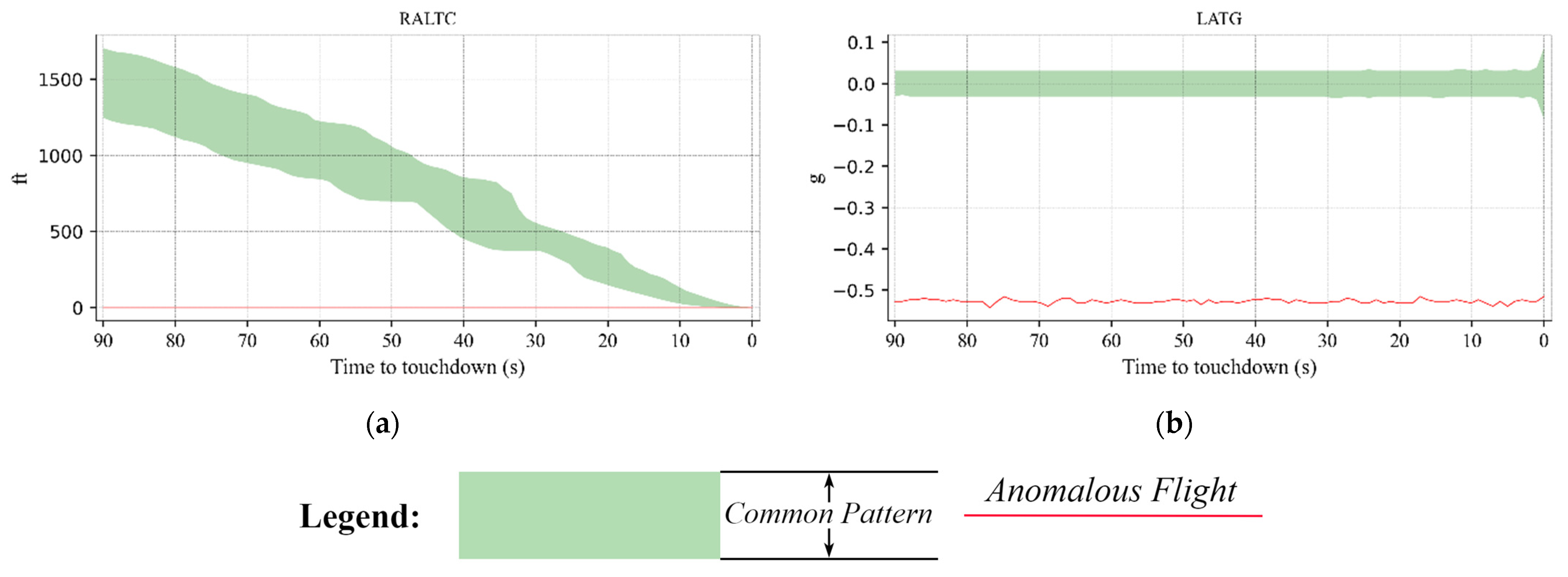
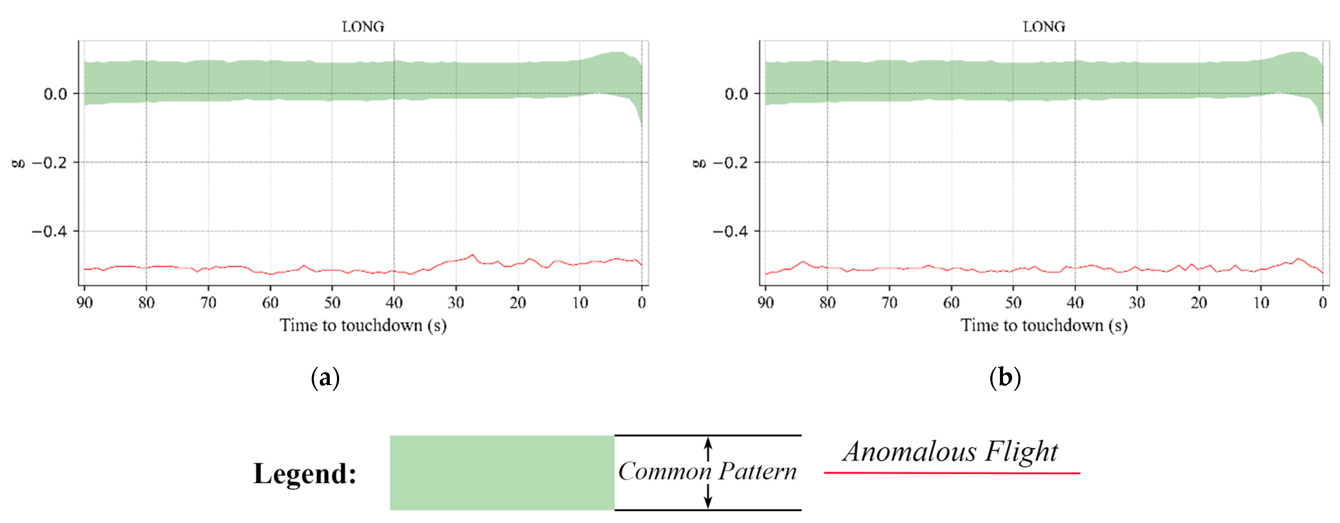
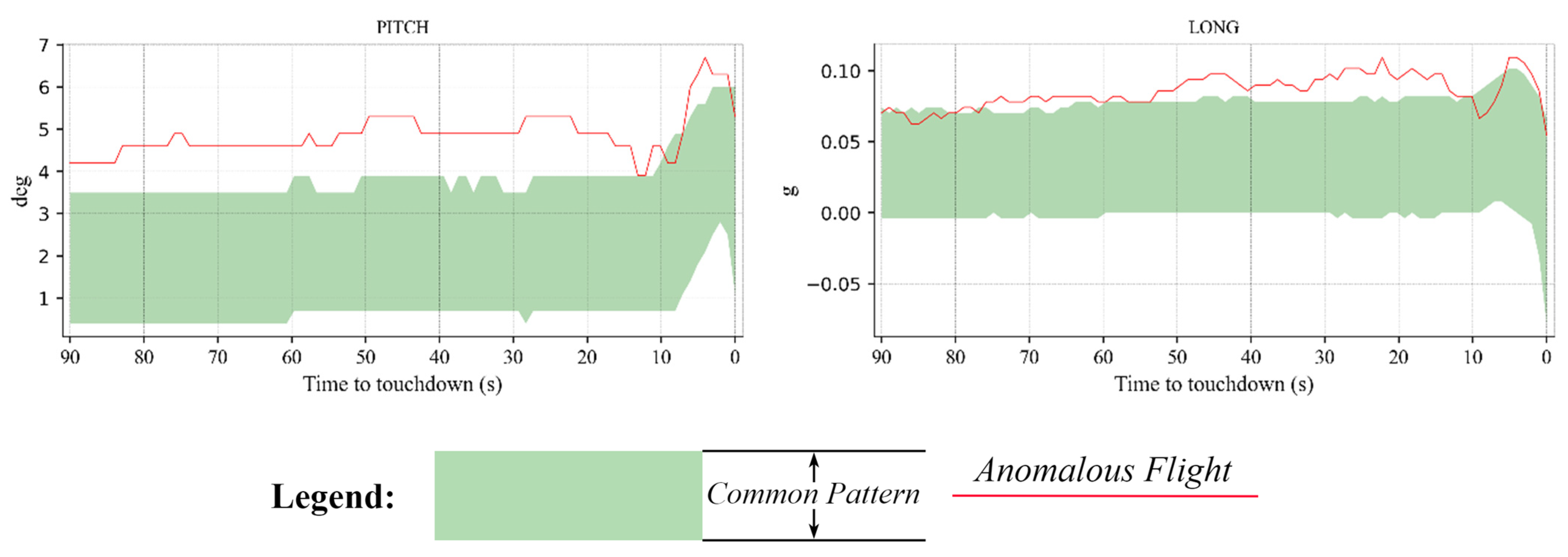
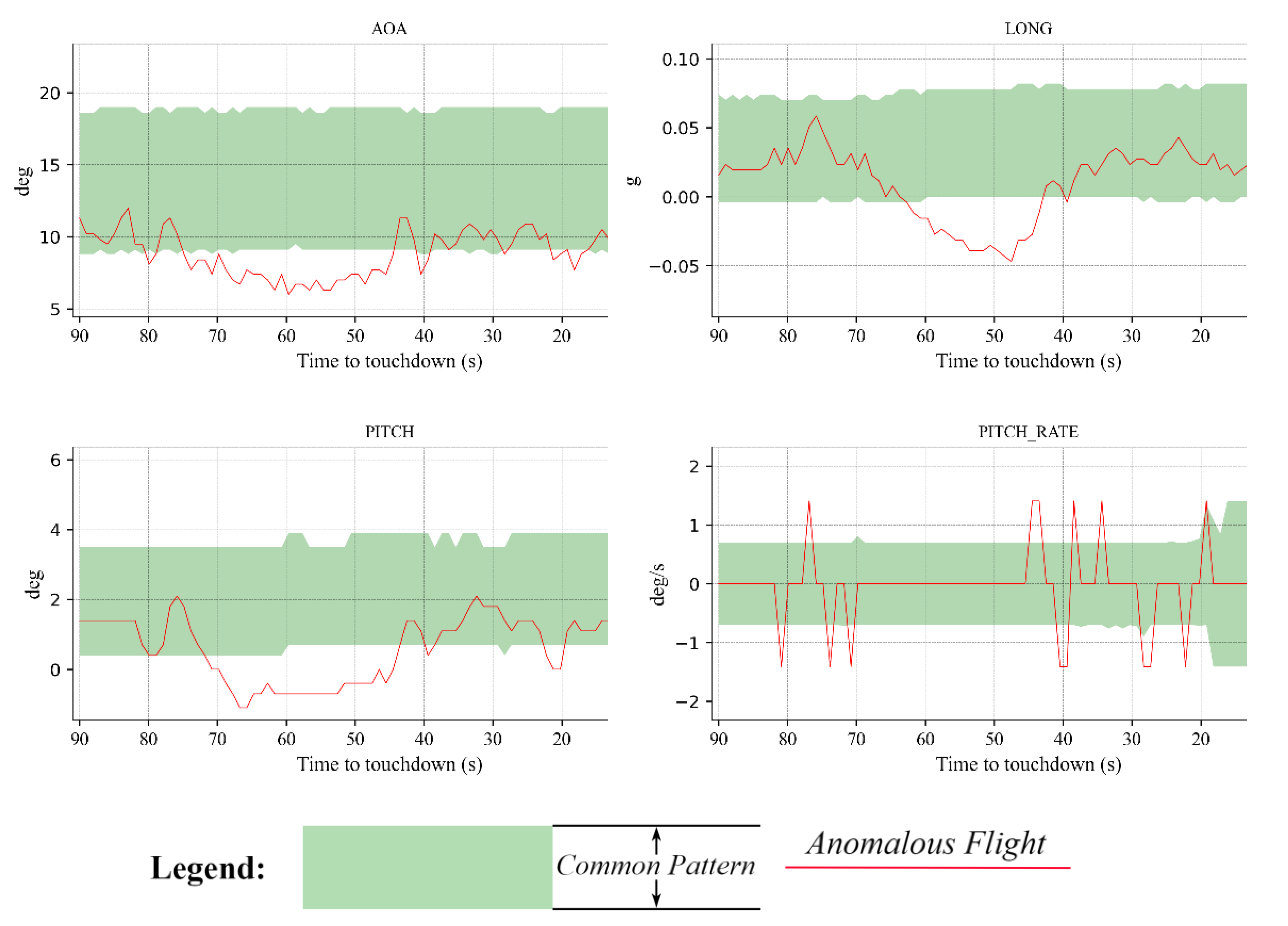
3.5. Anomalous Flights Detected during the Landing Phase

In this section, the characteristics of anomalous flights with operational significance for each airport are further analyzed in detail. As mentioned above, an aircraft landing at a certain airport will follow the specific landing procedure for that airport, and an anomalous flight landing at a given airport may be normal according to the flight procedure of another airport. Therefore, the assessment and analysis of anomalous flights should be performed in the airport where a flight lands. For this, all the flights are first divided according to the two airports, and the example anomalous flights of each airport are separately presented in detail.

For each example, the most distinctive flight parameters are presented in graphs with the same format, where the red lines denote anomalous flight patterns, and the light green band depicts the common flight landing pattern of each airport (the normal part in the clustering result).

3.5.1. Examples of Anomalous Flights That Landed at the ZPPP Airport

In this section, flights within the $O_1$ and $O_2$ collections that landed at the ZPPP airport are taken as examples to explain in detail the characteristics of the anomalous flights and the flight marked with point $P_1$. For the $O_1$ collection, in which all the flights have the same unusual behavior, a flight is plotted as a representative to show the details of the collection anomaly, as shown in Figure 11a. To be specific, $O_1$ is a collection of anomalous flights with flight altitude error records. The calibrated radar altitudes of all the flights were recorded as 0 throughout the landing phase.

Figure 11b shows the anomalous flight marked with point $P_1$, which is the furthest deviation from the landing pattern at the ZPPP airport. During the entire landing phase of the flight, the lateral acceleration G-Force was much lower than the common pattern, with values below −0.5.

The two flights within anomaly collection $O_2$ have extremely similar anomalous behavior as presented in Figure 12. They had been landing with a lower power; more specifically, the longitudinal acceleration G-forces of the two flights were much lower than the common pattern with values below −0.4 during the entire landing phase.

3.5.2. Examples of Anomalous Flights That Landed at the ZUUU Airport

Two examples of anomalous flights that landed at the ZUUU airport are separately displayed in Figure 13 and Figure 14. Figure 13 shows a flight landing with a higher elevation and a larger longitudinal acceleration. The pitch was always much larger than the common elevation angle, although it returned to normal between approximately 8 and 5 s before touchdown. From approximately 80 s before touchdown, the longitudinal acceleration was greater than the common pattern until approximately 10 s before touchdown; it briefly returned to the common range from approximately 10 s to approximately 5 s before touchdown but then increased above the normal pattern until touchdown.

As opposed to the flight mentioned above, a flight landing with a fluctuating attitude and dynamics that are lower than the common pattern is shown in Figure 14. To be specific, the AOA, PITCH, LONG, and PITCH_RATE fluctuated throughout the landing phase, with PITCH_RATE being the most pronounced. Separately, the angle of attack was lower than the common pattern from approximately 75 s to approximately 45 s before touchdown and fluctuated back and forth at the lower limit of the normal range during the subsequent landing. As the result of the larger change rate, the flight pitched up and down with a larger range in the two time periods of 85 to 65 s and 45 s to touchdown. Moreover, the flight landed with the head of the aircraft below the horizontal line from 70 to 45 s before touchdown because its angle of pitch was less than 0. In addition, the longitudinal acceleration was always smaller than the common pattern from approximately 62 s to approximately 42 s before touchdown.

4. Conclusions

In the field of civil aviation, safety management has shifted from post-event investigation and analysis toward advanced warning with the aim of effectively preventing potential accidents before they occur. For this, civil aviation strives to innovate and proactively identify operationally significant safety events that are untracked and then implement risk mitigation in the form of revising safety requirements to address the newly identified vulnerability. To improve and automate the identification of unknown vulnerabilities in flight operations, we proposed a time-feature attention mechanism that focuses on the key parameters and times and constructed a hybrid model for identifying operationally significant anomalies. The hybrid model combines TFA-CAE, which extracts flight features, and an HDBSCAN clustering algorithm to automatically detect anomalies based on the extracted features. The time-feature attention mechanism is demonstrated to improve the performance of flight feature extraction by comparing the TFA-CAE with SA-CAE (self-attention-based CAE), GRU-AE and PCA. In the subsequent detection and analysis of anomalies, flight patterns that are consistent with those at each airport are discovered, resulting in the anomalies being interpreted according to the corresponding pattern. Moreover, the hybrid model can also discover the aggregation of anomalous flights with similar unusual behaviors.

Future work: In this study, the flight patterns at the airport level and the corresponding anomalous flights were well discovered and detected, respectively; the next steps will potentially focus on developing an architecture to further discover the flight patterns at the runway level and detect the corresponding anomalous flights for airports with multiple runways. In addition, the automatic capture and classification of the same anomaly characteristics is another area of research that can enable better-targeted risk prevention.

References

- Memarzadeh, M.; Matthews, B.; Avrekh, I. Unsupervised Anomaly Detection in Flight Data Using Convolutional Variational Auto-Encoder. Aerospace 2020, 7, 115. [Google Scholar] [CrossRef]
- Qing, W.A.; Kaiyuan, W.U.; Zhangt, T.; Yi’nan, K.O.; Weiqi, Q.I. Aerodynamic modeling and parameter estimation from QAR data of an airplane approaching a high-altitude airport. Chin. J. Aeronaut. 2012, 25, 361–371. [Google Scholar]
- Chandola, V.; Banerjee, A.; Kumar, V. Outlier detection: A survey. ACM Comput. Surv. 2007, 14, 15. [Google Scholar]
- Hawkins, D.M. Identification of Outliers; Chapman and Hall: London, UK, 1980. [Google Scholar]
- Bach, F.R.; Lanckriet, G.R.; Jordan, M.I. Multiple kernel learning, conic duality, and the SMO algorithm. In Proceedings of the Twenty-First International Conference on Machine Learning, Banff, AB, Canada, 4–8 July 2004; p. 6. [Google Scholar]
- Lanckriet, G.R.; Cristianini, N.; Bartlett, P.; Ghaoui, L.E.; Jordan, M.I. Learning the kernel matrix with semidefinite programming. J. Mach. Learn. Res. 2004, 5, 27–72. [Google Scholar]
- Tax, D.M.; Duin, R.P. Support vector domain description. Pattern Recognit. Lett. 1999, 20, 1191–1199. [Google Scholar] [CrossRef]
- Li, L.; Das, S.; Hansman, R.J.; Palacios, R.; Srivastava, A.N. Analysis of Flight Data Using Clustering Techniques for Detecting Abnormal Operations. J. Aerosp. Inf. Syst. 2015, 12, 587–598. [Google Scholar] [CrossRef] [Green Version]
- Chalapathy, R.; Chawla, S. Deep learning for anomaly detection: A survey. arXiv 2019, arXiv:1901.03407. [Google Scholar]
- Javaid, A.; Niyaz, Q.; Sun, W.; Alam, M. A deep learning approach for network intrusion detection system. Eai Endorsed Trans. Secur. Saf. 2016, 3, e2. [Google Scholar]
- Peng, H.K.; Marculescu, R. Multi-scale compositionality: Identifying the compositional structures of social dynamics using deep learning. PLoS ONE 2015, 10, e0118309. [Google Scholar] [CrossRef]
- Tuor, A.; Kaplan, S.; Hutchinson, B.; Nichols, N.; Robinson, S. Deep learning for unsupervised insider threat detection in structured cybersecurity data streams. In Proceedings of the Workshops at the Thirty-First AAAI Conference on Artificial Intelligence, San Francisco, CA, USA, 4–9 February 2017. [Google Scholar]
- Wold, S.; Esbensen, K.; Geladi, P. Principal component analysis. Chemom. Intell. Lab. Syst. 1987, 2, 37–52. [Google Scholar] [CrossRef]
- Cortes, C.; Vapnik, V. Support-vector networks. Mach. Learn. 1995, 20, 273–297. [Google Scholar] [CrossRef]
- Liu, F.T.; Ting, K.M.; Zhou, Z.H. Isolation forest. In Proceedings of the 2008 Eighth IEEE International Conference on Data Mining, Washington, DC, USA, 15–19 December 2008; pp. 413–422. [Google Scholar]
- Reddy, K.K.; Sarkar, S.; Venugopalan, V.; Giering, M. Anomaly Detection and Fault Disambiguation in Large Flight Data: A Multi-modal Deep Auto-encoder Approach. Annu. Conf. Progn. Health Monit. Soc. 2016, 8, 7. [Google Scholar]
- Zhou, C.; Paffenroth, R.C. Anomaly Detection with Robust Deep Autoencoders. In Proceedings of the 23rd ACM SIGKDD International Conference on Knowledge Discovery and Data Mining (KDD ’17), Halifax, NS, Canada, 13–17 August 2017; pp. 665–674. [Google Scholar]
- Xu, H.; Chen, W.; Zhao, N.; Li, Z.; Bu, J.; Li, Z.; Liu, Y.; Zhao, Y.; Peii, D.; Feng, Y.; et al. Unsupervised Anomaly Detection via Variational Auto-Encoder for Seasonal KPIs in Web Applications. In Proceedings of the 2018 WorldWideWeb Conference, Lyon, France, 23–27 April 2018; pp. 187–196. [Google Scholar]
- An, J.; Cho, S. Variational Autoencoder based Anomaly Detection using Reconstruction Probability. Spec. Lect. IE 2015, 2, 1–18. [Google Scholar]
- Zimmerer, D.; Kohl, S.A.; Petersen, J.; Isensee, F.; Maier-Hein, K.H. Context-encoding variational autoencoder for unsupervised anomaly detection. arXiv 2018, arXiv:1812.05941. [Google Scholar]
- Zenati, H.; Foo, C.S.; Lecouat, B.; Manek, G.; Chandrasekhar, V.R. Efficient gan-based anomaly detection. arXiv 2018, arXiv:1802.06222. [Google Scholar]
- Li, D.; Chen, D.; Goh, J.; Ng, S.k. Anomaly Detection with Generative Adversarial Networks for Multivariate Time Series. arXiv 2018, arXiv:1809.04758. [Google Scholar]
- Schlegl, T.; Seeböck, P.; Waldstein, S.M.; Schmidt-Erfurth, U.; Langs, G. Unsupervised Anomaly Detection with Generative Adversarial Networks to Guide Marker Discovery. In Information Processing in Medical Imaging; Niethammer, M., Styner, M., Aylward, S., Zhu, H., Oguz, I., Yap, P.T., Shen, D., Eds.; Springer International Publishing: Cham, Switzerland, 2017; Volume 10265, pp. 146–157. [Google Scholar]
- Hinton, G.; SAlakhutdinov, R. Reducing the Dimensionality of Data with Neural Networks. Science 2006, 313, 504–507. [Google Scholar] [CrossRef] [Green Version]
- Kingma, D.P.; Welling, M. Auto-Encoding Variational Bayes. arXiv 2013, arXiv:1312.6114. [Google Scholar]
- Rezende, D.J.; Mohamed, S.; Wierstra, D. Stochastic backpropagation and approximate inference in deep generative models. In Proceedings of the 31st International Conference on Machine Learning (ICML-14), Beijing, China, 21–26 June 2014; pp. 1278–1286. [Google Scholar]
- Blei, D.M.; Kucukelbir, A.; McAuliffe, J.D. Variational Inference: A Review for Statisticians. J. Am. Stat. Assoc. 2017, 112, 859–877. [Google Scholar] [CrossRef] [Green Version]
- Basora, L.; Olive, X.; Dubot, T. Recent advances in anomaly detection methods applied to aviation. Aerospace 2019, 6, 117. [Google Scholar] [CrossRef] [Green Version]
- Goodfellow, I.; Pouget-Abadie, J.; Mirza, M.; Xu, B.; Warde-Farley, D.; Ozair, S.; Courville, A.; Bengio, Y. Generative adversarial nets. In Proceedings of the Neural Information Processing Systems Conference 2014, Montreal, QC, Canada, 8–13 December 2014; pp. 2672–2680. [Google Scholar]
- Schlegl, T.; Seeböck, P.; Waldstein, S.M.; Langs, G.; Schmidt-Erfurth, U. f-AnoGAN: Fast unsupervised anomaly detection with generative adversarial networks. Med. Image Anal. 2019, 54, 30–44. [Google Scholar] [CrossRef] [PubMed]
- Campello, R.J.; Moulavi, D.; Sander, J. Density-based clustering based on hierarchical density estimates. In Proceedings of the Pacific-Asia Conference on Knowledge Discovery and Data Mining, Gold Coast, QLD, Australia, 14–17 April 2013; Springer: Berlin/Heidelberg, Germany, 2013; pp. 160–172. [Google Scholar]
- Wang, L.; Wu, C.; Sun, R. An analysis of flight Quick Access Recorder (QAR) data and its applications in preventing landing incidents. Reliab. Eng. Syst. Saf. 2014, 127, 86–96. [Google Scholar] [CrossRef]
- Robert, F.S. Flight Dynamics; Princeton University Press: Princeton, NJ, USA, 2015. [Google Scholar]
- Federal Aviation Administration. Airplane Flying Handbook (FAA-H-8083-3A); Skyhorse Publishing Inc.: New York, NY, USA, 2011.
- Mnih, V.; Heess, N.; Graves, A. Recurrent models of visual attention. In Advances in Neural Information Processing Systems; Curran Associates, Inc.: Red Hook, NY, USA, 2014; pp. 2204–2212. [Google Scholar]
- Ba, J.; Mnih, V.; Kavukcuoglu, K. Multiple object recognition with visual attention. arXiv 2014, arXiv:1412.7755. [Google Scholar]
- Bahdanau, D.; Cho, K.; Bengio, Y. Neural machine translation by jointly learning to align and translate. arXiv 2014, arXiv:1409.0473. [Google Scholar]
- Xu, K.; Ba, J.; Kiros, R.; Cho, K.; Courville, A.; Salakhudinov, R.; Zemel, R.; Bengio, Y. Show, attend and tell: Neural image caption generation with visual attention. In Proceedings of the International Conference on Machine Learning, Lille, France, 6–11 July 2015; pp. 2048–2057, PMLR. [Google Scholar]
- Liu, M.; Li, L.; Hu, H.; Guan, W.; Tian, J. Image caption generation with dual attention mechanism. Inf. Process. Manag. 2020, 57, 102178. [Google Scholar] [CrossRef]
- Jaderberg, M.; Simonyan, K.; Zisserman, A. Spatial transformer networks. arXiv 2015, arXiv:1506.02025. [Google Scholar]
- Hu, J.; Shen, L.; Sun, G. Squeeze-and-excitation networks. In Proceedings of the IEEE Conference on Computer Vision and Pattern Recognition, Salt Lake City, UT, USA, 18–23 June 2018; pp. 7132–7141. [Google Scholar]
- Woo, S.; Park, J.; Lee, J.Y.; Kweon, I.S. Cbam: Convolutional block attention module. In Proceedings of the European Conference on Computer Vision (ECCV), Munich, Germany, 8–14 September 2018; pp. 3–19. [Google Scholar]
- Bai, S.; Kolter, J.Z.; Koltun, V. An Empirical Evaluation of Generic Convolutional and Recurrent Networks for Sequence Modeling. arXiv 2018, arXiv:1803.01271. [Google Scholar]
- Gorokhov, O.; Petrovskiy, M.; Mashechkin, I. Convolutional neural networks for unsupervised anomaly detection in text data. In Proceedings of the International Conference on Intelligent Data Engineering and Automated Learning, Guilin, China, 30 October–1 November 2017; Springer: Cham, Switzerland, 2017; pp. 500–507. [Google Scholar]
- Peter, J.H. “Robust Estimation of a Location Parameter”; Breakthroughs in statistics; Springer: New York, NY, USA, 1992; pp. 492–518. [Google Scholar]
- Ester, M.; Kriegel, H.P.; Sander, J.; Xu, X. A density-based algorithm for discovering clusters in large spatial databases with noise. Kdd 1996, 96, 226–231. [Google Scholar]
- Malzer, C.; Baum, M. A Hybrid Approach to Hierarchical Density-based Cluster Selection. In Proceedings of the 2020 IEEE International Conference on Multisensor Fusion and Integration for Intelligent Systems (MFI), 14 September 2020; pp. 223–228. Available online: https://doi.org/10.48550/arXiv.1911.02282 (accessed on 18 May 2022).
- Ankerst, M.; Breunig, M.M.; Kriegel, H.P.; Sander, J. OPTICS: Ordering points to identify the clustering structure. ACM Sigmod Rec. 1999, 28, 49–60. [Google Scholar] [CrossRef]
- Gupta, G.; Liu, A.; Ghosh, J. Automated hierarchical density shaving: A robust automated clustering and visualization framework for large biological data sets. IEEE/ACM Trans. Comput. Biol. Bioinform. 2008, 7, 223–237. [Google Scholar] [CrossRef]
- Pei, T.; Jasra, A.; Hand, D.J.; Zhu, A.X.; Zhou, C. DECODE: A new method for discovering clusters of different densities in spatial data. Data Min. Knowl. Discov. 2009, 18, 337. [Google Scholar] [CrossRef]
- Sander, J.; Qin, X.; Lu, Z.; Niu, N.; Kovarsky, A. Automatic extraction of clusters from hierarchical clustering representations. In Proceedings of the Pacific-Asia Conference on Knowledge Discovery and Data Mining, Seoul, Korea, 30 April–2 May 2003; Springer: Berlin/Heidelberg, Germany, 2003; pp. 75–87. [Google Scholar]
- McInnes, L.; Healy, J. Accelerated hierarchical density-based clustering. In Proceedings of the 2017 IEEE International Conference on Data Mining Workshops (ICDMW), IEEE, New Orleans, LA, USA, 18–21 November 2017; pp. 33–42. [Google Scholar]
- McInnes, L.; Healy, J.; Astels, S. hdbscan: Hierarchical density based clustering. J. Open Source Softw. 2017, 2, 205. [Google Scholar] [CrossRef]
- Prim, R.C. Shortest connection networks and some generalizations. Bell Syst. Tech. J. 1957, 36, 1389–1401. [Google Scholar] [CrossRef]
- Galler, B.A.; Fisher, M.J. An improved equivalence algorithm. Commun. ACM 1964, 7, 301–303. [Google Scholar] [CrossRef]
- Vaswani, A.; Shazeer, N.; Parmar, N.; Uszkoreit, J.; Jones, L.; Gomez, A.N.; Kaiser, Ł.; Polosukhin, I. Attention is all you need. Adv. Neural Inf. Process. Syst. 2017, 30, 5998–6008. [Google Scholar]
- Moulavi, D.; Jaskowiak, P.A.; Campello, R.J.; Zimek, A.; Sander, J. Density-based clustering validation. In Proceedings of the 2014 SIAM International Conference on Data Mining, Philadelphia, PA, USA, 24–26 April 2014; pp. 839–847. [Google Scholar]
- Rousseeuw, P.J. Silhouettes: A graphical aid to the interpretation and validation of cluster analysis. J. Comput. Appl. Math. 1987, 20, 53–65. [Google Scholar] [CrossRef] [Green Version]
- Davies, D.L.; Bouldin, D.W. A cluster separation measure. IEEE Trans. Pattern Anal. Mach. Intell. 1979, 1, 224–227. [Google Scholar] [CrossRef]