1. Introduction
The improvement of technology in Micro Electronics Mechanical Systems (MEMS), particularly in sensors and microcontrollers, encourages researchers to work on multi-rotors. They are in high demand, as evidenced by a large number of research studies. It has features such as simplicity to build easier maneuverability but also myriad applications that are sometimes not easy to perform for a man and, in extreme cases, are out of a human’s ability [
1]. For example, surveillance, package delivery, mapping, exploration, smart agriculture [
2], etc., are some applications that are used to be considered futuristic projects for human beings two decades ago, while these are not wondrous anymore rather than the reality. Interestingly, since all these applications primarily deal with trajectory tracking, the robotic community is continuously working on improving multi-rotors tracking performance to ensure smooth and collision-free flights [
3].
The quadrotor is one of the most widely chosen multi-rotors among researchers because of its being compact in size and light in weight. It has a cross-configured structure with two pairs of rotors facing opposite directions. It takes flight by balancing the thrust and torque produced by the rotors. Roll, pitch, yaw, and upward–downward push are the necessary operations for quadrotor movement.
The numerous applications of quadrotors can be divided into civilian and military categories, attracting academics’ interest in learning more about them. Aerial photography, inspections of industrial pipelines [
4], traffic monitoring, crop monitoring, fire detection, rescue operations, weather forecasting, news coverage, and other civilian applications are available, while military applications include border patrol, surveillance, and warfare [
4]. It is worth mentioning that a quadrotor is normally not fit for carrying heavy objects since it has only four rotors that are not able to generate a sufficient amount of thrust. Thus, in those cases, hexacopters or octocopters receive the interest of the researchers.
A quadrotor is designed using fixed-pitch rotor blades that offer Vertical Take-Off Landing (VTOL), and therefore, it does not require a runway. The quadrotor is an inherently unstable and under-actuated plant. The quadrotor frame is represented as a rigid body with three translational and three rotational degrees of freedom (DoF). When the quadrotor is used for outdoor applications, additional challenging operational requirements emerge, such as high agility, smooth maneuverability, disturbance rejection, payload variation, etc. Hence, different control strategies have been introduced in control engineering that can ensure promising performance during its operations.
In order to improve quadrotor tracking performance while taking environmental factors into account, studies have introduced controllers such as Proportional–Integral–Derivative (PID), Linear Quadratic Regulator (LQR), Backstepping, Feedback Linearization Control (FLC), Sliding Mode Control (SMC), Model Predictive Control (MPC), Linear Quadratic Gaussian (LQG), neural network, H-infinity, fuzzy logic, adaptive control, etc. These controllers are divided into three categories: linear, nonlinear, and learning-based controllers [
5,
6,
7,
8]. Interestingly, numerous works on linear control systems on quadrotor platforms are available since they are easy to design and employ [
9]. In addition, several studies have introduced another type of controller, hybrid controllers [
10], that include two or more different control strategies together to improve different aspects of the performance of the quadrotor.
Parrot mini-drone is a widely known commercial quadrotor platform for educational purposes, particularly to learn the quadrotor’s behavior in both indoor and outdoor environments. This platform is equipped with some sensors such as an ultrasonic sensor, an altimeter, an inertial measurement unit (IMU), and a camera that can describe its behaviors in different environments. It has received popularity because of its simplicity and ready-made platform at a reasonable price. Moreover, its Simulink software package is officially available, and hence, researchers can work on low-level control to test the performance in practice, which can lead to enhancing its tracking performance further. As a result, several works on controllers have been found on this platform. For example, Everett works on both LQR and LQI controller and conclude that LQI ensures better flight than regular LQR since LQI can reduce the steady-state error [
11]. Glazkov and Golubev introduce an adaptive control to observe the tracking performance of the mini-drone and receive a satisfactory performance in terms of following the reference trajectory [
12]. Castañeda and Gordillo adopt adaptive sliding mode control, where the adaptive approach is considered primarily to reduce the chattering problem of SMC. Thus, the platform achieves stability even in the presence of external disturbance and, at the same time, manages to follow the trajectory [
13,
14].
MPC, a nonlinear controller, has achieved popularity because of its robustness in tracking through dealing with noise, disturbance, and model uncertainty in quadrotor platforms. MPC and decentralized MPC are not so common for solving drone stabilization problems, and their main application is for flock optimal trajectory planning [
3]. While flight control is responsible for basic self-stabilization and maneuver, flocking coordination is responsible for inter-drone synchronization.
In this study, this platform is considered to compare the tracking performances of three different controllers, such as PID, LQR, and MPC. The main contribution of this work is to introduce MPC on the parrot mini-drone in tracking the trajectory and evaluate its tracking performance with the other controller on this platform.
2. Parrot Mini-Drone
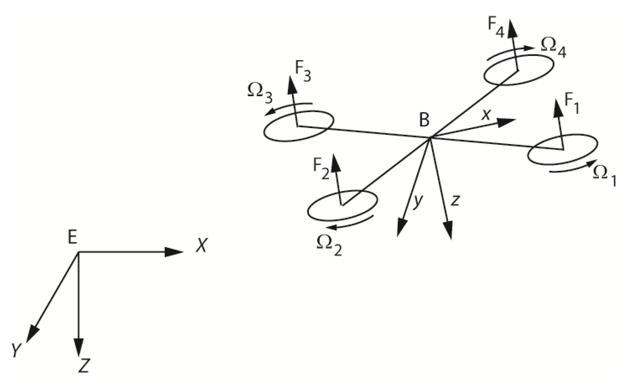
The Parrot mini-drone is a palm-sized quadrotor that can be controlled with a smartphone or a computer, making it very popular among researchers. It is a quadrotor of 55 g in weight and with three axes gyroscope, three axes accelerometer, a pressure sensor, and a 0.3-megapixel downward-facing camera of 60 fps. A 550 mAh Lithium-Polymer battery ensures a 6–8 min flight duration. Similar to regular quadrotors, four independent BLDC rotors with fixed pitched propellers are mounted at the four corners of this platform. Two of the four propellers rotate clockwise direction, while the other two rotate counterclockwise, as indicated in
Figure 1.
The dynamics of a quadrotor are generally described considering two frames of reference—an Earth-fixed frame (denoted with E) and a body frame (denoted with B)—as shown in
Figure 1. We assume that the origin of the body-fixed reference frame is at the quadcopter’s center of gravity, where the inertial measurement unit (IMU) is situated. Since the quadrotor frame is accelerating and rotating during its course of motion, the body-fixed reference frame is non-inertial. The Earth-fixed reference frame is assumed to behave as an inertial. The consideration of the Earth frame is required for the specification of the quadcopter’s geographic position and of the gravitational force direction. The Body-fixed reference frame hosts the rotor thrust forces and the angular velocities of the quadrotor.
2.1. Kinematics
The kinematics of a model establishes the relationship between the motion of the body-fixed reference frame (B) and the axes of the Earth-fixed reference frame (E). Hence, to explain the quadrotor’s kinematics, a transformation matrix is necessarily considered that can map any vector from the body frame into the Earth frame. As a result, a transformation matrix,
, is introduced, as illustrated in Equation (1), which is later used to express the Newton-Euler equations.
where,
, and
denote
,
and
trigonometric functions for some arbitrary angle
, and
,
,
denote rotation matrices around body frame principal axes. In addition, another transformation matrix
is required to describe the relationship between Euler rates,
, and the measured angular velocity vector of the quadrotor,
, as follows [
15,
16]
2.2. Dynamics
Quadrotor’s motion can be decomposed into a translational motion and a rotational motion. The orientation of the quadcopter in space is represented by the roll, pitch, and yaw rotations. When the drone is airborne and if its frame is tilted slightly, then translational motions along the X and Y axes arise, which are measured in the unit of meters as x, and y, respectively. Apart from that, the ascending or descending motion of the drone can be achieved by increasing or decreasing the average rotor speed [
17].
To facilitate stabilizing controller design, typically, an actuator decoupling matrix is selected depending on the frame configuration. The matrix in (3) for the Parrot Mambo ‘X’ drone frame maps the four squared speed references
,
,
and
To the lift force and stabilizing torques as
where
is the lift force along the body
dimension,
is the roll torque,
is the pitch torque, and
is the yaw torque. The control system can calculate the squares of the speed references with the help of a decoupling matrix, which is an inverse to the map from Equation (3), such that the decoupled manipulated variables
,
,
,
to correspond to the lift force and stabilizing torques. Therefore, in this case,
,
, and
, will be responsible for the roll, pitch, and yaw movements, respectively, whereas,
will be responsible for the upward or downward movement along the
z axis. The decoupling quality will depend on the symmetries between motor responses, blade geometries, and frame rigidity. Alternatively, since the mapping (3) is linear, the control system may drive the motor references directly by setting
. The relation between decoupled,
and direct,
, manipulated variables is the inverse of (3) and becomes
Table 1 shows the inertial parameters of the quadrotor.
Notably, the quadrotor dynamics can be described considering the Newton-Euler equation that deals with both forces and moments on the quadrotor. Here, the Equation (5) describes the translational motion of the quadrotor, while the Equation (6) describes the rotational motion of the quadrotor:
where
. From Equations (1), (2), (5), and (6), the complete mathematical model of the quadcopter can be derived as follows:
Finally, the dynamical model of the quadcopter can be described by four control inputs, and by twelve state variables, grouped in a state vector . Pay attention that Equations (7)–(15) are nonlinear due to the presence of trigonometric functions and multiplication between state variables. However, those nonlinear functions are smooth and allow linear approximations in the mini-drone flight envelope.
3. Control Strategies
3.1. PID-Based Control
PID control technique has been practiced on quadrotor platforms greatly because the quadrotor control channels can be naturally decoupled, and also, a PID controller allows for direct tuning of its parameters according to the performance requirements. Since the drone model is a Multiple Input Multiple Output (MIMO) system, a cascaded interconnection of several PID algorithms is required. The inputs to the controller have desired drone coordinates . For the PID design, it is more convenient to choose the decoupled variables, , for controller outputs, then use the Equation (4) to calculate the rotor speed references, , afterward.
At the core of the quadrotor, the PID control systems is an attitude stabilization controller, as shown in Equation (16)
where
,
are the pitch and roll attitude errors,
is the estimated pitch angle,
is the estimated roll angle,
and
are the estimated pitch rate and roll rates. The integral terms,
and
, of the controller are calculated as
where
is the discrete sample time of the control algorithm. Equation (17) is an approximation of the pitch and roll integrated errors, designed with a slightly smaller than unity pole to prevent wind-up effects. The pitch and roll reference signals
are generated by a position PID controller, which tries to minimize the position errors
and
between reference coordinates
and the estimated drone position
. The matrix,
, accounts for the drone yaw and
is a saturation nonlinearity set at
3 m. Along the altitude dimension, the total motor torque
is calculated as:
where
is a take-off gain,
is the reference altitude,
is the estimated vertical speed,
is the estimated drone altitude. Finally, a yaw PID controller calculates the torque around the vertical axis:
where
is the estimated yaw angle and
is the estimated yaw rate.
As it can be seen, the PID control strategy depends on a set of tunable gains, which determine the closed-loop stability and performance. Even though a lot of methods for PID tuning exist, the majority of them target single input single output systems (SISO). Furthermore, even after the selection of the initial gains, manual fine-tuning of the controller parameters is always advised. In our situation, we employed an optimization approach based on the nonlinear drone model provided in the preceding section to tune the PID controller gains.
3.2. Linear Quadratic Regulator
Because of its capacity to deal with MIMO systems, LQR is a common controller on quadrotor platforms. To reduce control effort, this controller uses a cost function minimizing approach from the optimal control theory. According to the LQR algorithm, a linearized model is required. Therefore, the quadrotor model is linearized at its hovering point denoted with
, where
and
. The deviations around the selected operating point are denoted with
and
such that
The purpose of LQR is to find a feedback gain matrix
K to calculate the control signal as
such that following quadratic functional
to be minimized, where
Q is a semi-positive definite square matrix of dimension n × n, and
R is a positive definite square matrix of dimension m × m, wherein n = 12 is the number of states, and m = 4 is the number of control inputs. Therefore, the closed-loop control system can be represented with
Controller gain is calculated as
where
P is a solution of the discrete-time algebraic Riccati equation
In order to construct an LQR controller for the mini-drone, the nonlinear model of drone motion must be expressed in discrete-time state-space coordinates of the form:
The vector
represents the set of linearized system states—position coordinates (
), velocities (
), Euler angles (
) and angular rates (
). The input signals used to stabilize the quadrotor are represented with the vector
. The sample time is chosen to be
ms. The operating point for the linearized model is numerically trimmed such that the mini-drone is held stable by hovering about 1 m above the ground. The resultant discrete-time linearized model, which is an approximate of the nonlinear model, expressed with (7)–(15), for the hovering operating point, is described with the equations:
The above Equations (29)–(40) should not be confused with their nonlinear counterparts (7)–(15), which were presented above. In the linearized model for the LQR design, there is no need to employ the decoupled controls because they are linearly dependent on rotor speed references . As it can be seen, the linearized model is chain-like due to sparse A and B, with control inputs acting directly on angular rates and on the vertical translation rate. All four inputs affect these states; hence, the controller aims to decouple these dependencies.
We have performed analytic linearization and time discretization of the nonlinear model for the specified hovering operating point. The quadrotor model linearization is a more-or-less standardized procedure; hence, we did not provide all the details of it. However, it can be extensively investigated with respect to approximation accuracy, which is a topic for another study. Our experiments with the drone show that the implementation of the MPC is very sensitive to the numerical roundings in the plant linear model. Hence the matrices of the linearized model are rounded in the following way to improve the numerical stability of the iterative procedure.
In order to obtain matrices
Q and
R, Bryson’s rule is used (
Table 2). The following are the weights for each state while determining the
Q matrix for LQR design:
The resulting matrix
Q is with elements only on the main diagonal denoted as:
where
,
,
,
and
. The matrix
, where
is the identity matrix of the fourth order, and the state feedback matrix,
K:
3.3. Model-Predictive Controller
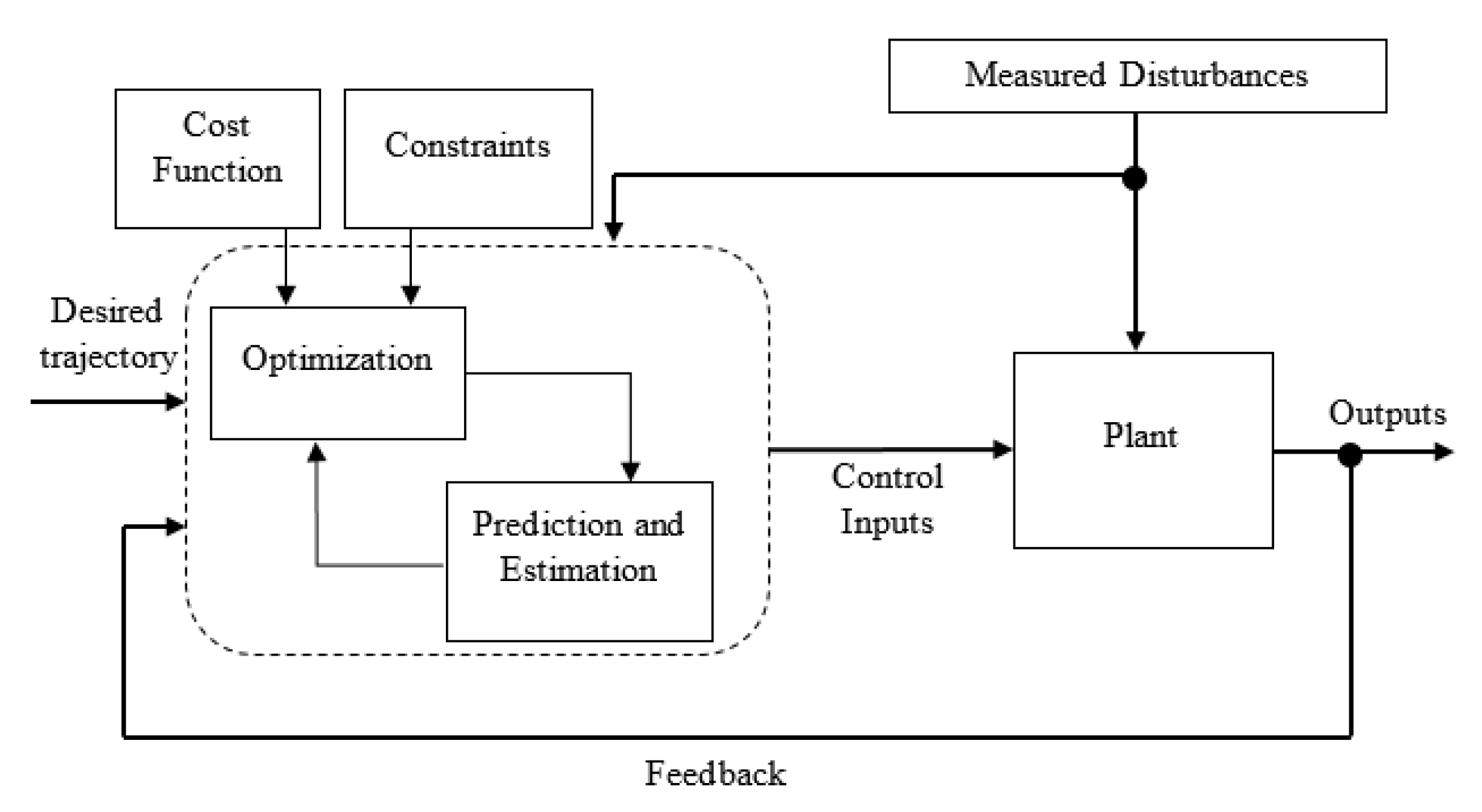
MPC for quadrotor platforms is gaining popularity in control engineering because it includes characteristics such as handling control constraints, state estimation, predictive behavior, noise, and disturbance rejection. More specifically, MPC gained popularity as a result of its predictive behavior, which may reduce closed system uncertainty [
19]. MPC employs the following steps (
Figure 2):
Construct a discrete-time state-space model.
Over a predefined prediction horizon, it predicts future plant states and outputs for a given control signal sequence over a predefined control horizon.
Quadratic optimization procedure selects a control sequence, which minimizes the closed-loop cost function.
Only the first sample from the optimal control signal is applied to the plant.
The method is then repeated from step 2 sequentially.
3.3.1. Plant Model
The design procedure of MPC takes the linearized discrete-time mini-drone model, specified with Equations (29)–(40), for the hovering operating point. The MPC continually predicts the behavior of the states within a prediction horizon,
N [
16], as
where
is the predicted state
sample steps after the present moment
,
are the future values of the control signal,
and
are the matrices of the linearized system (28).
3.3.2. Control Design
The MPC optimizer minimizes a quadratic cost function using two different weighting matrices
and
of appropriate dimension, which can be stated as
where
are the desired state values. Unlike the quaternion orientation-based quadrotor model, the Euler angle-orientation-based quadrotor model uses algebraic subtraction to determine the cost function; hence, this equation can be used to directly reduce the cost function [
20,
21,
22]. Quadratic programming is used to solve optimization problems by minimizing the cost function in a feasible search direction
[
23,
24].
3.3.3. Constrain Handling
In general, a motor has the ability to generate a certain amount of force that relies on the rpm and propeller design parameters. As a result, the control inputs are bound to the limit of motors’ properties in generating forces. Hence, the constraints must be considered at control input to design the control algorithm properly. However, when an upper bound, , and a lower bound, , at the control inputs where . The numerical representation of the discrete-time state-space model is for the fixed sample time of 5 ms. However, simulations of the nonlinear model with various MPC designs confirmed that required prediction horizon to achieve stable flight conditions was between 40–50 samples, with a control horizon of roughly 5 samples. However, the hardware platform running the controller implementation at the Parrot mini-drone did not allow such high order of prediction and control horizons due to insufficient resources. Hence, to reduce the prediction horizon samples, we decided to resample the discrete time state space model with a sample time of Ts = 100 ms. That way, the required prediction horizon for successful hover is about 10 samples, and the control horizon is about 2 samples. This is a limitation coming from what the Parrot Mambo drone microcontroller can sustain without violating real-time execution constraints; hence, it can be understood as a hardware limitation. The resampling operation over the state space model is achieved with the help of Tustin bilinear approximation. The match of the resampled and the original model is checked in the time and frequency domain for the frequencies up to 5 rad/s.
In the presented MPC design prediction horizon is set to 10 samples, and the control horizon is set to 2 samples. The nominal control vector, U = (237–237 237–237), and the nominal state vector Y = 0 correspond to the selected operating point of the linearized model. All control inputs are saturated in the bounds [10 500] for motors 1 and 3 and in the bounds [−500 −10] for motors 2 and 4. The weights for the control signal are set to and control signal rates weights are set to 0.0005. The weights are set to these values through iterative experimentation with the Parrot Mambo drone. However, these values are not the only possible stabilizing solution.
The critical for the control performance is the value of the state weights. In the present design, we assume all states are measurable as
Output weights vector is normalized to a unit vector. A white noise model is assumed to act on all outputs with a variance 0.01. That is introduced to smooth further the generated controller signal. Since the MPC design will be implemented in real-time, that requires tight bounds on the optimization iterations. As a result, sub-optimal solutions are tolerated, and the maximum number of iterations is limited to 10.
4. Simulation Results
The controller variants are evaluated in simulation as well as in experiments. Typically controller performance is best understood in the frequency domain. However, the MPC is a nonlinear control approach, and frequency response has to be obtained through approximation. Since there is not a unique way to define such approximation, that will be a question for separate research. Therefore, we decided to compare the controllers in the time domain alone in this study.
The desired drone trajectory is selected as a rectangular path, which is stretched by a low-frequency sinusoidal wave in each spatial dimension to increase the trajectory complexity. The resultant trajectory is defined by the following expressions:
The yaw, pitch, and roll reference signals are held at zero. At low altitudes, the ground rotor effect is strongly disturbing the stability of the drone; hence, initially, take-off power impulse is applied to the motors such that commanded torque is
, where
is empirically selected take-off gain.
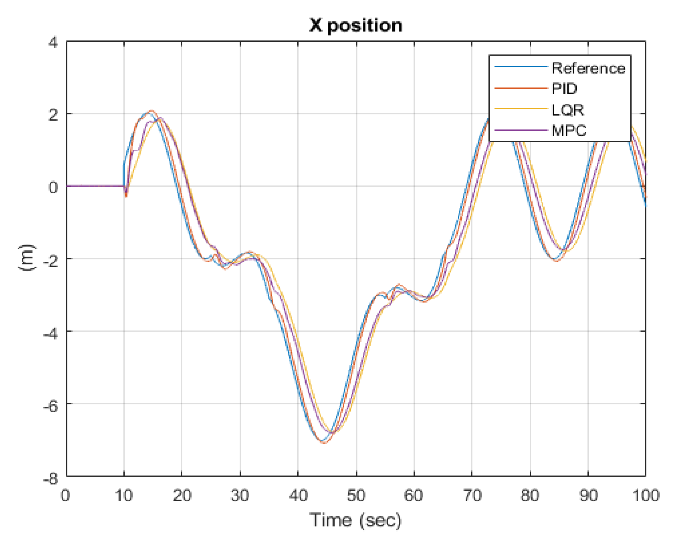
Figure 3 overviews the comparison between PID, LQR, and MPC drone control systems during tracking of the desired trajectory. Both LQR and MPC demonstrate similar tracking performance keeping aircraft close enough to the reference. However, the PID-based closed-loop system response is oscillatory during some of the trajectory segments, even though the aircraft stability is recovered after that. During simulation, safety-critical sensor conditions for
flight zone boundaries and velocity estimation error
at
are monitored such that simulation stops if asserted. The velocity estimation error
is between velocity
from optical flow processing and velocity
from the complementary filter. None of the controllers drive the system close to these conditions, and the estimation errors of state coordinates are negligible. Landing is not simulated in this scenario; however, the controller handles landing by descending at a near ground altitude of −
, in which spinning down the rotors is safe for the drone.
Table 3 calculates 2-norms of the tracking errors between reference position signals and actual drone positions, as well as the 2-norms of the yaw, pitch, and roll angles, for the simulation duration
. The PID-based control system demonstrates the best tracking performance along with X and Y dimensions; however, it is worst along the critical for stability Z dimension. The drone altitude is tightly associated with averaged rotor velocity, which is determinant for the current operating point and respective linear approximation of the equations of motion. Along with the pitch and roll components, the PID-based controller is also with the worst performance compared to LQR and MPC systems. On the other hand, the LQR controller performs best in keeping drone orientation, such that for the yaw angle, the 2-norm is 10 times less for the LQR compared to the PID-based. The tracking performance along X, Y, and Z coordinates are similar for LQR and MPC closed loops, and the same is true for the pitch and roll angles. One drawback of the MPC is evident in the large yaw angle component compared to PIC and LQR. That does not affect the position tracking performance. Eventually, that yaw error can be minimized by modifying the respective weights during the specification of the MPC cost function.
Figure 3 shows the resultant trajectory of the drone center of gravity in Cartesian coordinates for the three examined controllers. It is clear that the PID-based controller is unable to keep the aircraft on track, particularly after take-off around position (0, 0). Furthermore, it can be seen that there is no significant difference in tracking performance between LQR and MPC controllers. This can be attributed to the similarity in cost criteria utilized in these controllers. Both LQR and MPC are based on the quadratic cost with state and control weighting matrices. However, in the case of LQR, the controller minimizes the quadratic cost over an infinite time horizon, and MPC solves the optimization problem iterative for the finite prediction horizon. According to the trajectory tracking experiment, the optimum performance is obtained when the drone altitude is close to the operational point value used to build the linearized model.
Figure 4 and
Figure 5 show the detailed transient response of the three controllers during trajectory tracking along the X and Y dimensions. Because the trajectory segments approximate a constant velocity reference signal, the steady state error will be proportional to the number of integrator elements in the loop. The PID-based control loop works with zero steady-state errors but with pronounced oscillations with amplitudes around
. The LQR and MPC work with a constant steady state error around
during constant velocity trajectory segments, which is the reason for the higher 2-norms of the respective tracking errors. However, the velocity error is zero, and the magnitude of the position error can be controlled with the slope of the position reference. Furthermore, the response of the LQR and MPC is not oscillatory. Generally, both controllers demonstrate quite similar behavior, which can be explained by the shared quadratic cost.
Figure 6 compares the altitude tracking performance between the controllers where two transients are most evident. The first is right after take-off when the −1.5 m operating height must be stabilized. Before lowering to the required altitude, a PID-based controller is characterized by a large overshoot of more than 50% or reaching –3.3 m. Due to developed overshot, the drone motors almost stop causing a free fall. With the LQR, the overshot is considerably damped to around 30%, and finally, with the MPC, the ascent is aperiodic without overshot. After reaching the operating altitude of –1.5 m a small sinusoidal reference variation is commanded. All controllers succeed in following that reference, but the transient for the PID-based controller is oscillatory.
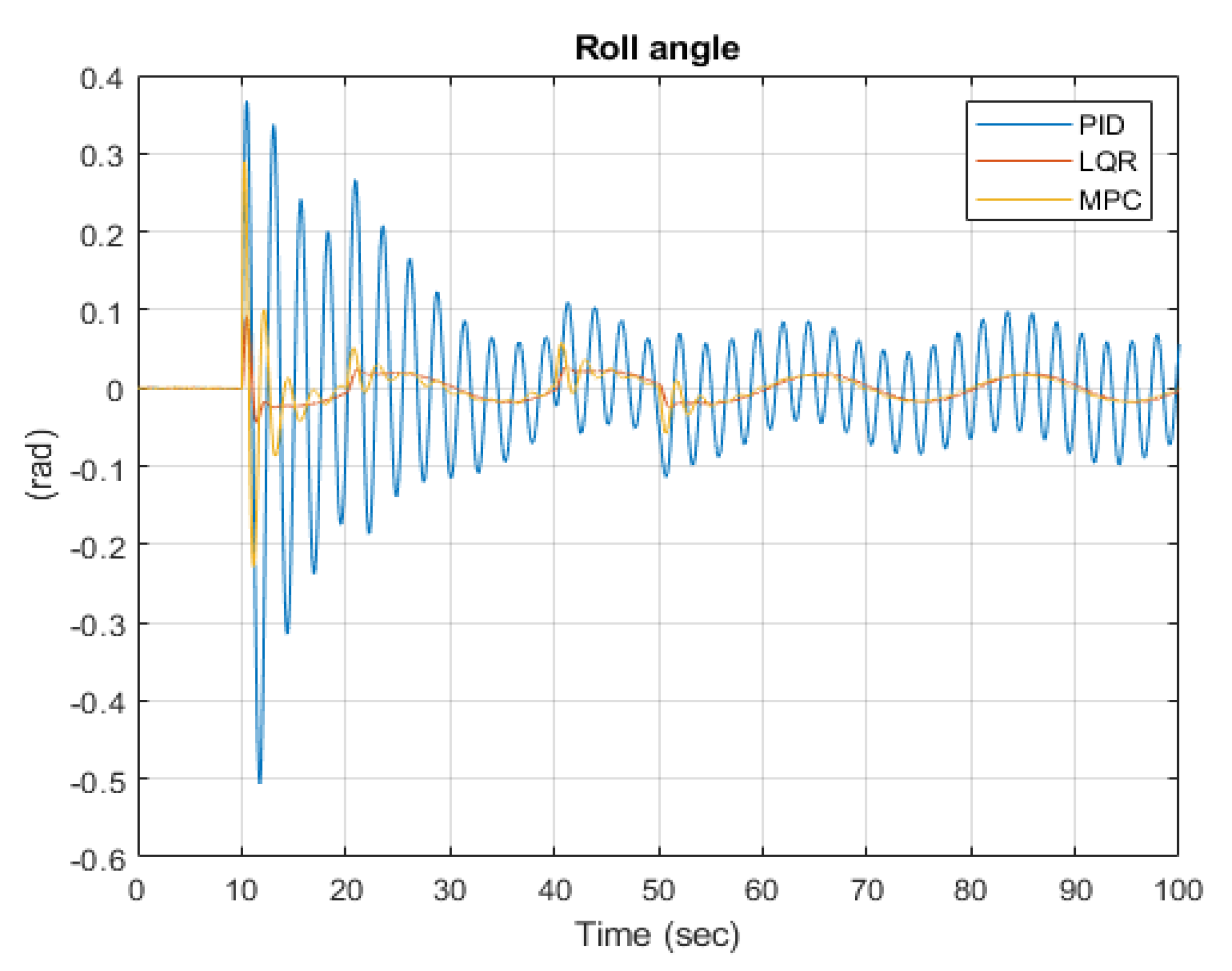
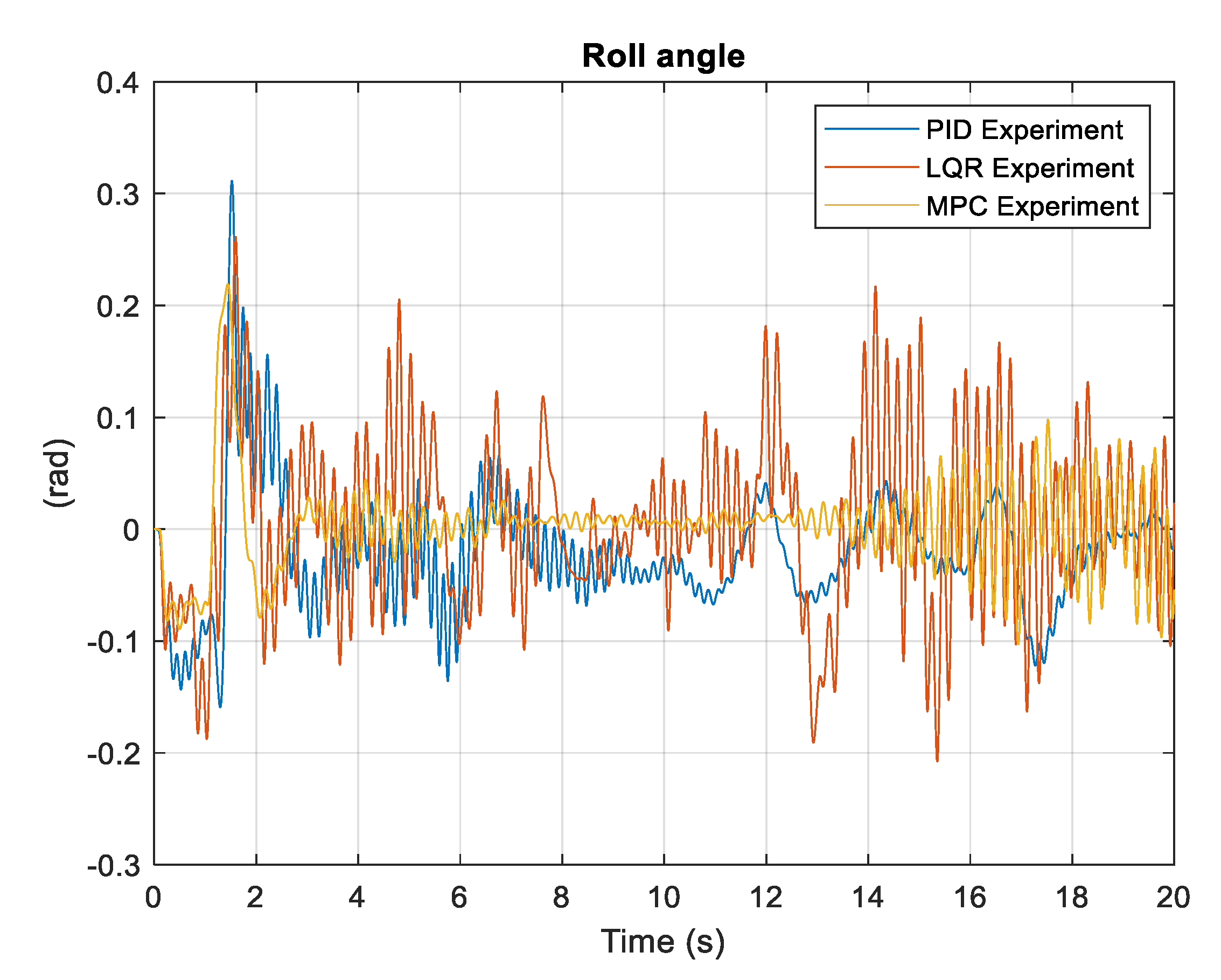
Figure 7 demonstrates the performance in roll angle stabilization for the controllers. On the one hand, small deviations in the roll and pitch angles are necessary to accomplish drone translation in Cartesian space, inducing a projection of the motor thrust vector along the horizontal plane. On the other hand, roll and pitch angle amplitudes are critical for aircraft stability in the presence of external disturbances such as wind, ground effects, asymmetries in rotor wakes, etc.
The PID-based closed-loop system’s behavior is highly oscillatory, as can be observed, with a steady state amplitude of roughly 0.1 rad and a frequency of about 0.4 Hz. Even though the aircraft remains stable, such oscillations indicate small stability margins. The control system based on LQR is aperiodic, with a maximum deviation of roughly 0.025 rad. Similar behavior is obtained with the MPC algorithm. However, small oscillations appear during transients along the trajectory with amplitude up to 0.05 rad.
Sensitivity of the closed-loop to disturbances is most evident after the take-off, where the control algorithm is enabled at t = 10 s in the presence of non-zero initial conditions for the plant due to impulsive motor trust required to lift the drone high enough to overcome the ground effect. Integral terms of the controller are still not developed. Hence, large swings in the roll and pitch angles appear. For the PID, maximal swing amplitude is as large as 0.5 rad, for LQR, it is 0.2 rad, and for MPC, it is 0.3 rad.
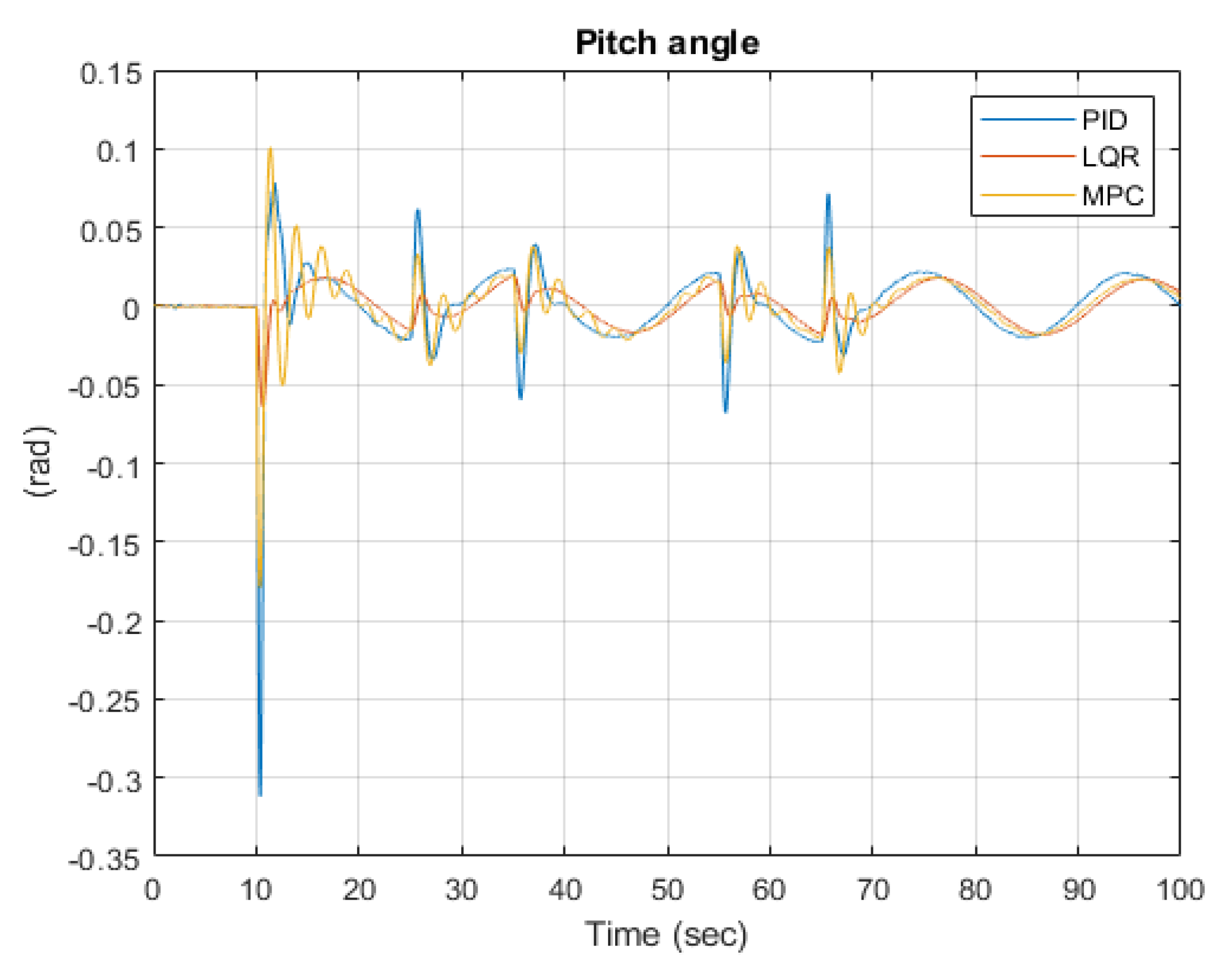
The simulated pitch angle is depicted in
Figure 8. As can be seen, the pitch angle variations using the PID-based controller are far fewer than those seen in the roll angle. This indicates that the cause of the PID oscillatory behavior is related to different drone inertia along pitch and roll axes. Hence, additional tuning of the PID could improve its performance. As noted in the introduction, a lot of PID tuning rules exist for SISO systems, but not so much for multivariate systems as is the case with the drone. On the contrary, tuning of the MPC- or LQR-based regulators is more direct with specifying weighting matrices for the output and control variables.
In the steady state, the maximal pitch deviation for the PID controller is 0.075 rad, for the LQR, it is 0.025 rad, and for the MPC, it is 0.04 rad. The maximum pitch deviation for the PID-based controller is 0.3 rad after the take-off impulse, 0.06 rad for the LQR, and 0.17 rad for the MPC.
5. Experimental Results
Figure 9,
Figure 10,
Figure 11 and
Figure 12 present the experimental results with the designed PID, LQR, and MPC controllers. For the implementation of the controllers in the Parrot Mambo mini-drone, the authors have employed the Simulink Coder Toolbox capabilities to automatically convert the controller model to the MISRA compatible C code. The generated code can be validated in software in the loop simulations. For the particular mini-drone, we are relying on the Mathworks supplied framework models for Parrot, which is extended with the developed controllers. We also provide the Simulink diagram used for code generation for the 3 controllers as a
Supplementary Material.
This framework model takes operator command, raw sensor signals, and image data from the drone camera as inputs and calculates the four motor speed reference commands. The sensor signals are composed of three accelerometer signals, three gyroscope signals, optical flow data, ultrasound altitude signal, and pressure signal. Accelerometer, gyroscope, and pressure data are first calibrated by removing the constant bias terms detected during sensor initialization. Low pass filters are applied to the accelerometer data and yaw rate data. Then the complementary filter estimates the mini-drone orientation from the accelerometer, gyroscope signals, and yaw estimate from the optical flow driver. The aim of the complementary filter is to produce a converging estimate for the drone orientation through minimization of the error between accelerometer or optical flow and gyroscope integrated Euler angles. The altitude and vertical speed are then estimated from orientation estimate, gravity vector, and ultrasonic signal through a Kalman filter. Furthermore, the translation velocity of the drone is estimated from the optical flow velocity estimate, altitude estimate, and orientation estimate. Finally, the drone position is estimated with the help of the Kalman filter by comparing the integrated velocity and optical flow estimate.
The following figures compare the experimental performance of the designed regulators. An important note is that experiments are performed indoors, which is well recognized that magnetometer, ultrasonic and optical signals can be disturbed. The general observation is that LQR and MPC controllers demonstrate similar performance, with MPC being a bit smoother in response.
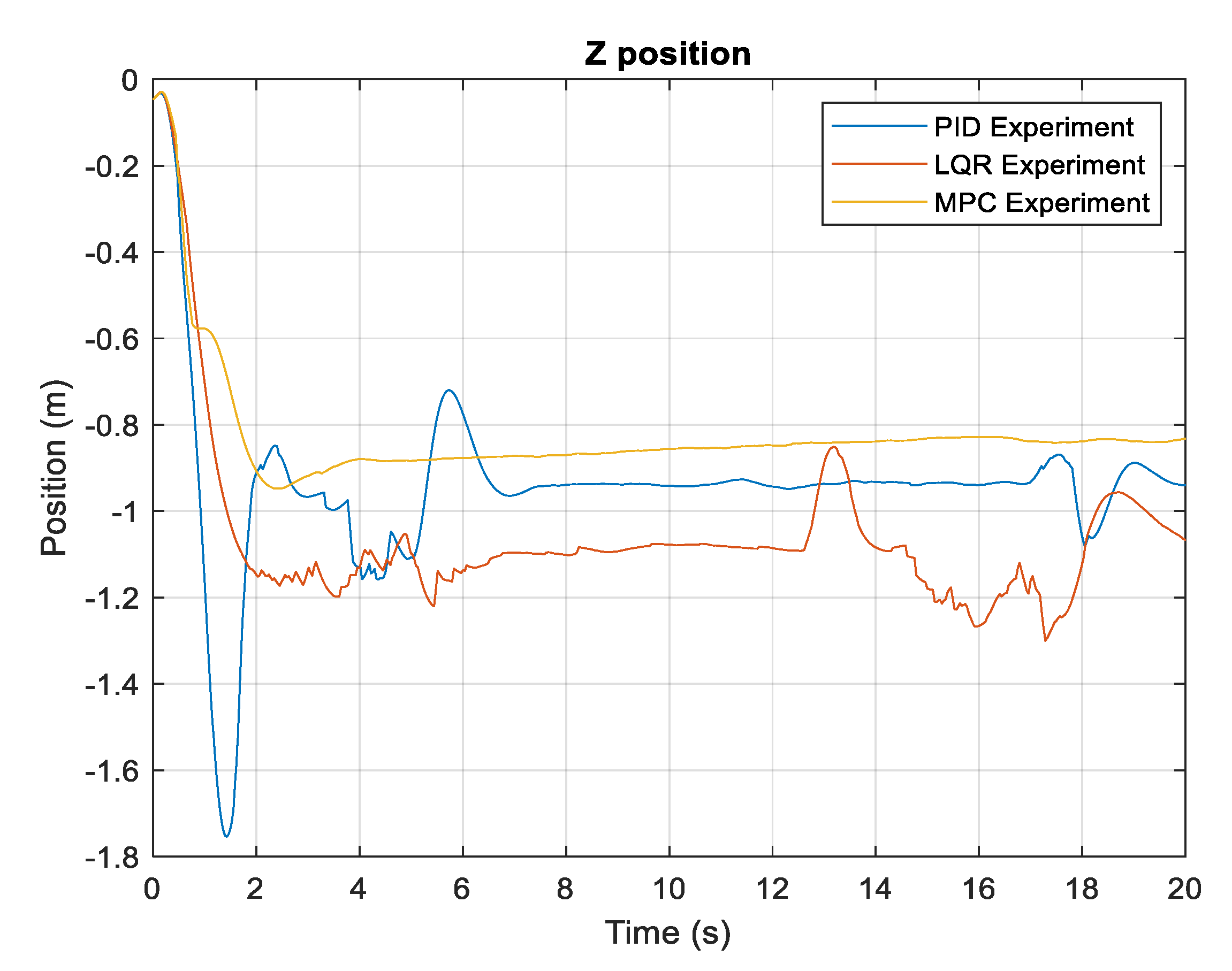
In
Figure 9, along the Z position, the PID hovering error is settled at around 20 cm; however, it is increasing. With the LQR or MPC controllers, the hovering error is steady at around 30 cm but with a decreasing trend.
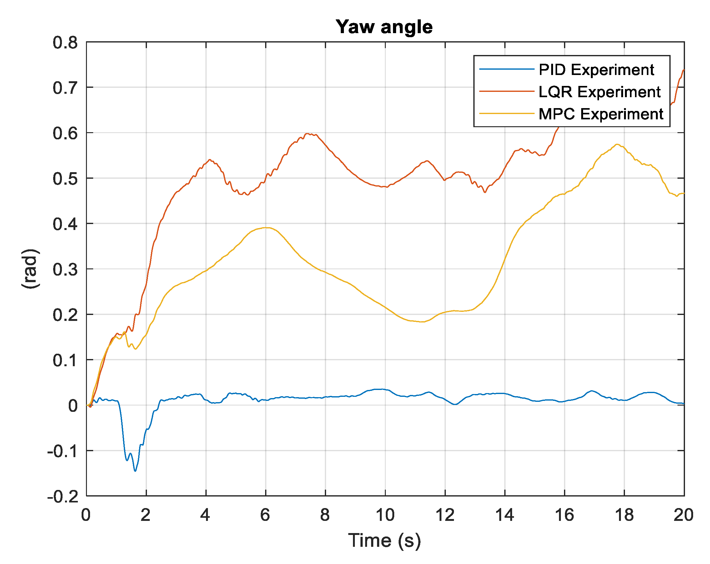
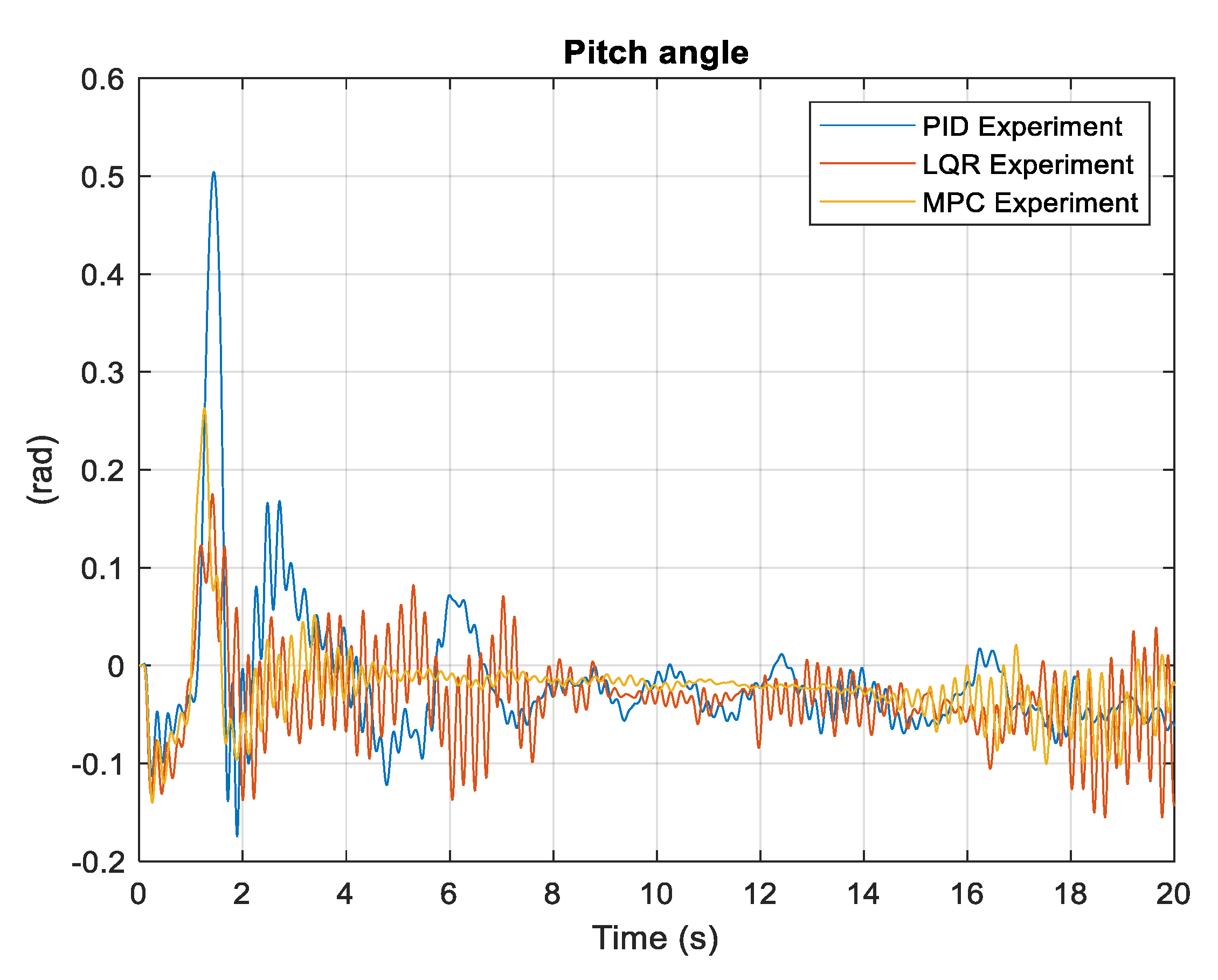
The controllers do not show the same response in their rotational motion as they show in simulation. PID controller shows significant overshoot in the pitch angle response and undershoots in yaw angle response. However, PID response is better compared to LQR and MPC in yaw movement. Along both roll and pitch movement, MPC and LQR show jittery responses, while PID is better in response compared to them.
This work introduces the simulated and experimental results of the Parrot mini-drone flight with three different controllers such as MPC, PID, and LQR. This study compares the performance of the controllers from several aspects such as tracking error, stability, and robustness. From the tracking error aspect in simulation, LQR performs well compared to PID and MPC. However, in terms of stability and robustness in real-time, MPC shows promising performance while both PID and LQR show fluctuations in their responses. Theoretically, MPC should perform well because it is a nonlinear controller and can estimate the system’s behavior. However, it could not show its strength since the Parrot mini-drone is a low-budget commercial quadrotor equipped with some sensors that are poor in response. Positions along the X and Y axes are measured by a camera instead of a GPS sensor, and hence, the responses become worse when it moves over a plane ground that is without a black-white box pattern. During the experiments, it was discovered that the sensor’s performance degrades over time, and so the quadrotor cannot be run for a longer period of time to fully appreciate the controller’s performance. In addition, the microcontroller that is used in this quadrotor is not suitably efficient to offer a suitable platform to show a controller’s strength effectively. As a result, environmental factors may greatly affect the quadrotor’s performance in that case where the controllers have limited opportunity to show their robustness. Thus, the system shows inconsistency in both simulated and experimental results.
Both MPC and LQR are suitable controllers for the quadrotor platform because they have six states that are controlled by four inputs. However, PID is suitable for dealing with the SISO system, and hence, X and Y positions are coupled with roll and pitch movement to be controlled by PID controllers, respectively, though finally, six different PID controllers have been adopted for the states. Hence, it is time-consuming to find out suitable gains. On the other hand, LQR is a low computational controller that relies on Q and R matrices.
MPC is a powerful nonlinear controller that can ensure stability and robustness to the system, and interestingly, in this experimental work, it offers stability in the system compared to the other controllers as well. It couples estimator with cost function approach that makes more computational, however. Hence, designing a suitable controller is not as stressful as PID.
6. Conclusions
In conclusion, PID, LQR, and MPC controllers have been applied to Parrot mini-drones, and their strengths and weakness have been analyzed in this platform. These controllers have been chosen considering the existing works where MPC on Parrot mini-drone is not available. The most important findings of this study can be summarized as:
- -
The employment of a PID-based controller on a quadrotor platform is straightforward, given the accumulated research on the topic. The PID approach is advantageous because it allows manual parameter tuning but does not provide a unified, systematic way to optimize the system performance. We do not claim that simulated and experimental PID performance will be as poor with all the possible parameter tunings. However, for our time spent tuning the PID controller, we could not find tunings that led to a better result. The tuning of multivariate PID controllers is mostly a heuristic task trying to balance the requirements of several feedback loops with the aim of keeping internal stability.
- -
The application of LQR for mini-drone stabilization is also extensively investigated on various platforms. It generally shows better performance in tracking and stability than PID-based controllers, which was confirmed by our simulations and experiments. The tuning of LQR requires less effort than tuning of PID because the existence of a solution to the algebraic Riccati equation guarantees the closed-loop stability. Interestingly, in experimental work, both MPC and LQR show similar tracking errors along the altitude.
- -
This work brings novelty to the Parrot Mambo platform by offering MPC and introducing its characteristics and suitability. This work substantiates that MPC can be considered to ensure the stability and robustness of the system; however, simulation work shows poor performance in tracking than LQR. The explanation can be found that LQR provides an infinite time horizon quadratic cost minimization, while the MPC is always limited to a finite time horizon. Moreover, the iterative nature of MPC solution calculation may not always converge to a solution that minimizes the cost function. Practical tuning of the MPC weights to run on a Parrot Mambo drone proved a very hard task, requiring a lot of experiments.
- -
The practical implementation of the proposed controllers was facilitated by the automatic code generation capabilities offered by the Simulink Coder. That mostly eliminated the need to perform lower-level system programming. The microcontroller installed in the Parrot Mambo drone is powerful enough to support each of the designed controllers. However, we have reached some limitations with the implementation of MPC. Due to its intensive computation requirements, we had to limit the prediction horizon to 10 samples and increase its sample time to 100 ms in order to perform a successful experiment. The LQR is far more efficient in implementation than MPC. The greatest benefit of MPC is that it allows explicit account for the control signal amplitude and rate constraints.
- -
A relatively large mismatch between the simulation and experimental results is evident in the present research. We have explored a vast number of controller parameter values, which led us to the conclusion that there is inherent uncertainty in the linearized model, which can explain the differences between the simulation and experimental results. That can be compensated by performing a special identification experiment with random signals to extract statistical estimates about model parameters or estimate a state-space model directly using subspace identification methods.


