Optimization of the Conceptual Design of a Multistage Rocket Launcher

Abstract

The design of a vehicle launch comprises many factors, including the optimization of the climb path and the distribution of the mass in stages. The optimization process has been addressed historically from different points of view, using proprietary software solutions to obtain an ideal mass distribution among stages. In this research, we propose software for the separate optimization of the trajectory of a launch rocket, maximizing the payload weight and the global design, while varying the power plant selection. The launch is mathematically modeled considering its propulsive, gravitational, and aerodynamical aspects. The ascent trajectory is optimized by discretizing the trajectory using structural and physical constraints, and the design accounts for the mass and power plant of each stage. The optimization algorithm is checked against various real rockets and other modeling algorithms, obtaining differences of up to 9%.

1. Introduction and State of the Art

Since the beginning of the space age, in 1957, access to space has become widespread. Although in 1966, only the USA, France, and the USSR had the capacity to send satellites into space using their own launch vehicles, today, the list of countries with such capacity has increased, including those involved in the Europe’s space agency, China, Iran, Ukraine, India, Israel, North Korea, Brazil, Japan, and New Zealand [1]. Manned missions have also received significant interest from both governments and the private sector: both world powers, such as China or the USA, have shown interest in taking human beings to new frontiers such as the Moon or Mars, and private companies, such as Virgin, SpaceX, or Blue Origin, are offering commercial flights around the Earth.

A rocket or launch vehicle carries a payload beyond Earth’s atmosphere, powered by a jet rocket engine. Depending on the mass of the vehicle, they can be classified in the following categories, shown in

Table 1. Classification of launch vehicles according to its mass.

Category	Mass (t)
Small	0–2
Midsize	2–20
Heavy	20–50
Super heavy	>50

[2]:

To increase launch efficiency and reduce costs, the following alternatives have historically been addressed:

• The use of a multistage rocket, as proposed by, among others, Tsiolkovsky. A SSTO (Single Stage to Orbit) would consume more fuel, but if complete reusability could be achieved, as in the case of an airplane, the cost savings would be significant. Unfortunately, the efficiency of the engines prevents their use in these scenarios. Multistage rockets increase performance, eliminating part of the mass that is no longer necessary during the ascent to orbit: By dividing the rocket into multiple zones or stages, we can reduce the size of these losses. Each stage will, thus, have a fraction of the total propellant, which can be optimized to maximize performance. Another advantage comes from the type of propellant: the first stages, being subjected to higher atmospheric pressures, have to withstand a greater aerodynamic drag, together with a substantial modification in the propulsive performance of the nozzle. High pressures present in the early stages require a shorter nozzle geometry, while in vacuum or at high altitudes, a more elongated shape is preferable for optimal performance. Therefore, this is one of the most remarkable advantages of the use of several stages since it allows to use different engines, depending on the external conditions, thus improving the overall efficiency of the rocket. Finally, a multistage rocket allows for the use of different propellants, depending on the stage. The first stages tend to use solid or liquid fuel based on hydrocarbons, which can achieve the great thrusts necessary to overcome the gravitational attraction, while being relatively low cost. For the following stages, the required thrust is substantially lower, as sub-orbital speeds are reached. In this way, fuels are chosen that admit a large specific impulse with a low volume. Therefore, in these stages, high efficiencies can be achieved without an excessive increase in cost [3]. On the contrary, for multistage rockets, one or more engines will be required at each stage, thus increasing the cost and structural fraction of the whole. The complexity of design and manufacturing also increases, leading to additional reliability issues.
• Optimization of launch parameters, among others: the mass distribution between the stages, the most suitable engine for each of them, the size and mass of the resulting rocket, the amount of propellant required, and the ascent path. All these factors interact with each other, so the optimal solution will be given by an adequate balance between all the elements.

Optimization of the climb path is of utmost importance in the process. Normally, starting with a vertical ascent from the launch pad, it usually continues with a turn to reach the horizontal speed necessary to start orbiting. The ascent is subject to gravity losses, aerodynamic losses, and steering losses. Controllability is affected by the fact that it is performed only with a vector thrust in most cases, and it undergoes the coupling of rotational dynamics to inertia, natural instability, and the presence of a non-minimum phase behavior [4]. In the process of optimizing the climb path, the potential applications include: maximizing the payload that can be sent to orbit, analyzing how design changes affect performance, and determining the launch window [5]. The optimization problem is not trivial: on the one hand, it is a non-linear dynamic system; there are discontinuities in state variables, time-dependent forces may exist, and some final conditions may not be explicitly known [6]. At the beginning of the space age, the approach to solving this optimization problem was dominated by the indirect methods (using the necessary analytical conditions obtained from the calculus of variations). However, from the end of the 20th century, the growth in the computational capacity of computers has allowed the use of direct methods on increasingly complex problems. The indirect methods use the calculus of variations to determine the optimality conditions of the problem, resulting in a multiple-point boundary-value problem [7]. By the use of the Euler–Lagrange equations, as well as the Pontryagin’s Maximum Principle (among others), conditions applying to the adjoint variables are reached. Possible examples of these methods include the indirect transcription and indirect shooting method.

The direct methods state the original optimization problem in an approximative manner, converting such a problem into a non-linear programming problem (NLP). Direct collocation, multiple shooting, or the pseudospectral methods are possible examples. Rao [7] and Betts [8] provide comprehensive surveys of the advantages and limitations of direct and indirect methods.

Both methods are still used nowadays, and each one complements the cadences of the other. Focusing on the indirect ones, it can be stated that Gath and Well, who developed an algorithm to provide good initial guesses for subsequent calculations [9], Pontani, with the optimization of an air-launch vehicle [10], and Filatyev and Yanova, with the optimization of branching ascent trajectories in presence of atmospheric disturbances [11], are the most significant, among some others.

Regarding the direct ones, possible examples are Brusch et al., who used the shooting method for the trajectory optimization of the Space Shuttle [12], Jänsch et al. for the Ariane 5 [13], Bollino, with the optimization of the reentry of the Lockheed Martin X-33 [14], or Zotes and Peñas, with the use of a genetic algorithm for the optimization of maneuvers [15].

According to the best of our investigations, only a few software packages provide relevant functionality in this area of optimization of rocket design and its trajectory. FONTSIZE, developed in the 90s, provides vehicle dimensioning and trajectory determination at the same time [16]. INTROS (integrated rocket sizing model), developed for NASA, allows dimensioning of the launch vehicle using MER (mass estimating relationships). POST (program to optimize simulated trajectories), developed in NASA, provides trajectory optimization under a three degrees of freedom approach. These software packages are restricted and cannot be used publicly. ASTOS (aerospace trajectory optimization software) is a project for the ESA that simulates trajectories and optimization for three and six degrees of freedom in many scenarios, including ascent and interplanetary maneuvers; as in the previous cases, it is not public domain. Finally, ASTER form Roscosmos, with an approach based on the indirect optimization of branched trajectories that describe the motion of the rocket, obtains multipoint boundary-value problems to solve. The program has proven to be capable of solving ballistic and control problems, for injection aid, in a flexible way [17].

In this research, we introduce an optimization software for the conceptual design of a launch rocket and its trajectory under various optimization techniques; the key properties are mass minimization for the take-off and payload mass maximization. The design optimization can provide configuration alternatives useful to assess the effect of design choices—especially on the propulsive plant—on the overall performance. The trajectory optimization, on the other hand, is designed to obtain fast results and prove the feasibility of a conceptual design in a preliminary phase, especially for the newer launch vehicles that carry smallsats. The paper is organized as follows: Section 2 provides a description of the mathematical model and algorithms used in this research; Section 3 shows how an implementation of those algorithms applies to different use cases; the conclusions are presented in Section 4, including the subsequent steps that will follow this work.

2. Materials and Methods

2.1. System Modeling

2.1.1. Cost Model

The Delta-V is used to evaluate the requirement of the mission, which, in turn, allows for calculating the fuel necessary to carry out that mission. This Delta-V needed for a mission can be obtained as:

$$\mathsf{\Delta }{V}_{mission}=\mathsf{\Delta }{V}_{orbit}+\mathsf{\Delta }{V}_g+\mathsf{\Delta }{V}_d+\mathsf{\Delta }{V}_p+\mathsf{\Delta }{V}_r+\mathsf{\Delta }{V}_{margin}$$

(1)

where the $\mathsf{\Delta }{V}_{orbit}$ refers to the speed that the rocket must reach in order to orbit the planet in a given orbit, and it is equal to the orbital velocity at the insertion point. Furthermore, the losses or gains related to the rotation of the Earth $\mathsf{\Delta }{V}_r$ can be expressed as:

$$\mathsf{\Delta }{V}_r=V_{orbit}-\sqrt{{\left(V_{orbit}\sin A_0-V_{r,h_0,{\varphi }_0}\right)}^2+{\left(V_{orbit}\cos A_0\right)}^2 }$$

(2)

where $V_{r,h0,\varphi 0}$ is the linear velocity of the Earth at that latitude and altitude, and $A_0$ is the launch azimuth. In prograde orbits, the rotation component will have a negative value, implying some help from the Earth to launch. Therefore, these two components can be calculated precisely.

The rest of the components, that is, the aerodynamic loss $\mathsf{\Delta }{V}_d$, propulsive losses $\mathsf{\Delta }{V}_p$, and associated losses to gravity $\mathsf{\Delta }{V}_g$, cannot be calculated until the final trajectory is known. Therefore, due to the inability to calculate the trajectory before knowing the design of the vehicle, they are estimated based on the works of [3,5,18,19,20]:

$$\begin{gathered} \mathsf{\Delta }{V}_g=750–1500 \mathrm{m}/\mathrm{s} \\ \mathsf{\Delta }{V}_d=40–150 \mathrm{m}/\mathrm{s} \\ \mathsf{\Delta }{V}_p=20–50 \mathrm{m}/\mathrm{s} \end{gathered}$$

(3)

Lastly, $\mathsf{\Delta }{V}_{margin}$ is a safety margin to take into account effects not analyzed or errors in the data. According to [21], it usually uses 2% of the total Delta-V.

2.1.2. Propulsive Model

The propulsive modeling is carried out from the characterization of a rocket engine. The optimization algorithm will have complete freedom to choose the engine, for each phase, from a database of 27 real engines, with its characteristics gathered in

Table 2. Engines of the last stages [21,22,23,24].

Engines	Propellant	Thrust [kN]	Specific Impulse (vac) [s]	Mixture Ratio	Expansion Ratio	Height [m]	Diameter [m]	Mass [kg]
11D58M	LO2/Kerosene	79.5	353	2.48	189	2.27	1.17	230
RD-0210	N2O4/UDMH	582	327	1.95	81.3	2.33	1.47	566
AESTUS	N2O4/MMH	30	325	2.05	84	2.2	1.32	111
J-2	LO2/LH2	890	426	5.5	28	3.38	2.01	1438
YF-75	LO2/LH2	79	440	5	80	2.8	1.5	550
LE-5B	LO2/LH2	137	447	5	110	2.78	2.15	269
HM7-B	LO2/LH2	70	447	5.14	83.1	1.8	1	155
VINCI	LO2/LH2	180	465	4.83	240	4.2	2.15	550
RL-10B	LO2/LH2	110	462	4.83	250	4.15	2.13	301

and

Table 3. Engines of the first stages [21,22,23,24]. The * symbol indicates an approximation due to lack of public data.

Engine	Propellant	Thrust [MN]	Specific Impulse (sl.) [s]	Mixture Ratio	Expansion Ratio	Height [m]	Diameter [m]	Mass [kg]
RD-170	LO2/Kerosene	7.65	310	2.6	36.87	3.78	4.02	9750
RD-180	LO2/Kerosene	3.82	311	2.72	36.4	3.56	3.15	5480
RD-107	LO2/Kerosene	0.81	257	2.06 *	18.86	2.578	1.85	1250
F-1	LO2/RP1	6.91	264	2.27	16	5.64	3.72	8391
MA-5A	LO2/RP1	1.84	263	2.25	8	3.43	1.19	1610
RS-27	LO2/RP1	0.91	263	2.245	8	3.63	1.07	1027
RD-253	N2O4/UDMH	1.47	285	2.67	26.4	3	1.5	1300
YF-20	N2O4/UDMH	0.76	259	1.95 *	10	2 *	0.84	712.5 *
Viking 6	N2O4/UH25	0.68	249	1.71	10.5	2.87	0.99	826
RS-68	LO2/LH2	2.89	360	4.83 *	21.5	5.2	2.43	6600
RD-108	LO2/Kerosene	0.78	252	2.77 *	18.9	2.86	0.67	1250
Viking 5C	N2O4/UH25	0.68	249	1.7	11	2.87	2.22	826
YF-20B	N2O4/UDMH	0.73	259	1.95 *	10	2 *	0.84	712.5
RS-68	LO2/LH2	2.89	360	4.83 *	21.5	5.2	2.43	6597
SSME	LO2/LH2	1.82	364	6	77.5	4.24	1.63	3177
RD-0120	LO2/LH2	1.51	359	6	85.7	4.55	2.42	3450
LE-7A	LO2/LH2	0.84	338	5.9	51.9	3.67	2 *	1800
Vulcain 2	LO2/LH2	0.94	320	6.7	61.5	3.6	2.1	811

. The following parameters are considered: (a) Thrust T; (b) Specific impulse Isp; (c) Mixing ratio; (d) Expansion ratio; (e) Height; (f) Diameter; (g) Mass.

In order to facilitate convergence, the engines are divided among those specific for the early stages of a rocket (characterized by a great thrust) and those typical of the last stages (with less thrust but greater efficiency). Once the algorithm chooses an engine from the data base, its multiplicity must be calculated so that the thrust-to-weight ratio is higher than that indicated by the optimization variable. Therefore, for each stage:

$$n_{engines}=ceil\left[\left(\frac{\left(\frac{T}{W}\right)W_{initial}}{T_{engine}}\right)\right]$$

(4)

$$T_{total}=T_{engine} n_{engines}$$

(5)

$${\left(\frac{T}{W}\right)}_{effective}=\frac{T_{total}}{W}$$

(6)

where $\frac{T}{W}$ is the thrust-to-weight ratio set by the optimization variable and ${\left(\frac{T}{W}\right)}_{effective}$ is the one of the rocket. To calculate the number of motors ($n_{engines}$), the ceiling function is used, so the actual thrust-to-weight ratio of the rocket is equal to or higher than that chosen by the optimization variable.

From the number of motors per stage, it is possible to define the diameter of the rocket. This diameter is considered constant and equal to the largest diameter required by a stage. In turn, for each stage, the diameter chosen is the greater of that required by the payload and by the motors, so it is used for the latter results of the packing of circles [25] for the calculation of the minor diameter needed. The diameter chosen is the minimum that the rocket geometrically needs, which does not imply that it is the most desirable. However, in the absence of a common criterion applicable, the smallest possible diameter is chosen. Once the engine is selected, the fuel and oxidant necessary for its operation are defined. This allows the calculation of their masses and volumes, by using the mixing ratio f, as well as the total propellant mass, $m_p$, the densities of the fuel, ${\rho }_{fuel}$, and the oxidant, ${\rho }_{oxidant}$, of the propulsive plant at each stage.

$$m_{fuel}=m_p f$$

(7)

$$v_{fuel}=\frac{m_{fuel}}{{\rho }_{fuel}}$$

(8)

$$m_{oxidant}=m_p-m_{fuel}$$

(9)

$$v_{oxidant}=\frac{m_{oxidant}}{{\rho }_{oxidant}}$$

(10)

The propellant tanks are considered in a tandem type of configuration, made up of a cylinder with half an ellipsoid on top of either end. The volume $V_{total}$ is then:

$$V_{total}=\pi R^2{h}_{cilinder}+2\frac{2\pi a b c}{3}$$

(11)

where $h_{cilinder}$ is the length of the cylindrical part of the tank, and $R$ is its radius. Moreover, a, b, and c are the semiaxes of the ellipsoid. In our case, a and b are equal to allow for the continuity of the tank. The height $h_{tank}$ is:

$$h_{tank}=\frac{\left(V_{total}-\frac{4\pi a b c}{3}\right)}{\pi R^2}+2c$$

(12)

And the area $S$ is:

$$S=2\pi a^2\left(\frac{h_{cilinder}}{a}+1+\frac{1-e^2}{e}\mathrm{atanh}\left(e\right)\right)$$

(13)

$$e^2=1-\frac{c^2}{a^2} with c<a$$

(14)

where $e$ is the eccentricity of the ellipse formed by the cross section. Using Equations (11) to (14), the height and area of the tanks can be determined, which will be useful for the calculation of the final geometry and the structural mass of the configuration.

2.1.3. Atmospheric and Gravitational Model

For atmospheric modeling, the NRLMSISE-00 (US Naval Research Laboratory Mass Spectrometer and Incoherent Scatter radar for Exosphere) model was chosen. This model was developed by the US Naval Research Laboratory in the year 2000, and it allows for the determination of dozens of atmospheric parameters from the surface up to 1000 km. For this, values for the date, latitude, longitude, and F10.7 flux are needed. Since, in a preliminary design, it is complicated to predict the launch window, the first of July of 2022 is selected as the date and the values of a standard day for the F10.7.

For the variation of gravity, an implementation of zonal harmonic planetary gravity, based on planetary gravitational potential, is used. The zonal harmonic coefficients J2, J3, and J4 are used.

2.1.4. Mass Model

To estimate the structural mass of the different rocket elements, Akin’s Mass Estimating Relationships, or MER [26], has been used to heuristically calculate the mass from information on the geometry of the rocket and the propellant tanks, as well as their capacity.

2.1.5. Aerodynamical Model

Aerodynamic characteristics are difficult to predict in the absence of CFD simulations or experimental methods, which are both impractical for an optimization process.

The following simplifications have been considered:

• The angle of attack is small, typically less than 10° in atmospheric flight.
• The flow is uniform around the rocket.
• The rocket is axisymmetric, which is the case in serial staged vehicles without fins. Thus, only serial rockets are considered on the trajectory analysis. However, if the vehicle has fins, an additional term can be added on (15) to take into account the additional drag, as described in the study of Caporaso [27].
• The lift is negligible.
• Induced drag is considered negligible.
• The variation in drag with the angle of attack is also negligible.

The total drag of the vehicle can then be divided as follows:

$$C_{D_{Total}}=C_{Dfb}+C_{Db}$$

(15)

where C_Dfb is the body drag, and C_Db is the base drag. C_Dbd is the component resulting from the sum of pressure drag and skin friction drag. The first can be expressed according to Caporaso [27]:

$$C_{Dfb}=\left[1+\frac{60}{{\left(\frac{l_{TR}}{d_b}\right)}^3}+0.0025\frac{l_b}{d_b}\right]\frac{ S_s}{S_m}{C}_f$$

(16)

where $l_{TR}$ is the total length of the rocket, $l_b$ the length of the cylinder, $l_c$ is the length of the boat tail (not applicable), $d_b$ is the maximum diameter, $C_f$ is the friction coefficient, $S_s$ is the wetted area, and $S_m$ the maximum frontal area. The friction coefficient is modeled through empirical laws, such as Schoenherr’s, with the compressibility corrections exposed in Hoerner [28].

The base drag can be described, according to Fleeman [29], as:

$$C_{Db}=\{\begin{array}{c}0.12+0.13M^2 if M<1\\ 0.25/M if M>1 \end{array}$$

(17)

Equation (16) is valid only in subsonic regime. Therefore, Caporaso [27] provides the following semi-empirical corrections in the case of a sharp-nosed vehicle:

$$\begin{array}{l}\frac{C_D}{C_{D_S}}=1.0+35.5{(M-0.9)}^2 if 0.9\le M\le 1.05 \\ \frac{C_D}{C_{DS}}=1.27+0.53\exp \left(-5.2\left(M-1.05\right)\right) if 1.05\le M\le 2\end{array}$$

(18)

where $C_{DS}$ is the value of the drag coefficient in subsonic regime, and M is the Mach number.

Therefore, in subsonic regime, Equations (16) and (17) are used to calculate the total drag coefficient. Once Mach 0.9 is reached, Caporaso [27] corrections are used to adapt the coefficient to transonic and subsonic (Equation (18)). In regimes greater than Mach 2, Equation (18) is still used despite being outside its validity domain, due to the little importance of drag to the heights at which these speeds are reached.

Any standard geometry with the tip not rounded can be considered. This choice affects the total wetted area $S_S$ of the rocket.

2.2. Algorithm Design

2.2.1. Optimization Algorithm

In the optimization process, the use of optimization algorithms is necessary to solve and speed up the problem. In our research, we chose to use the genetic algorithm to solve the optimization design problem (including the distribution of masses), whilst for the optimization of the trajectory, we selected Patternsearch. This is because both problems are non-smooth and, consequently, the algorithms based on gradients are not a good option.

The genetic algorithm is a metaheuristic algorithm and, therefore, stochastic, and evolutive, which is inspired by the process of evolution that occurs in nature to optimize a certain problem. This algorithm can provide near-optimal solutions, exploring the domain without the need of an initial guess. Due to its nature, a convergence to a minimum is not guaranteed. However, the solution calculated by the genetic algorithm could be refined by the use of a local solver with adequate convergence properties.

Patternsearch is a deterministic algorithm that is not based in gradients. The process is based on analyzing a series of points that are in the neighborhood of the current point, detecting in which one the objective function has a lower value compared to the one in the first point. This algorithm is chosen for the case of trajectory optimization due to its capacity to find optimal, or near optimal, solutions in a reasonable time without providing information about the gradient. According to [30], this algorithm is proven to be convergent under certain conditions. In both cases, MATLAB was used to find the solution.

2.2.2. Optimal Stage Distribution

For each configuration of the design parameters, the optimal distribution of the total mass in each stage is calculated; that is, their size, considering the mass ratio $n_i$, the exhaust velocity $V_{e,i}$, and the structural ratio ${ϵ}_i$ variable at each stage. Under these conditions, a numerical optimization of the problem is needed. Figure 1 displays a summary of the masses described in this section for a parallel configuration:

Considering, for an arbitrary stage $i$, $m_{pl,i}$ is the payload, which is the part of the vehicle that we want to send into space. Normally, there are fixed characteristics set by the customer, so from a design-oriented point of view, it is an input. $m_{p,i}$ is the propellant mass, consisting of the fuel and oxidant that is consumed to generate thrust. Finally, $m_{e,i}$ is the structural mass, which includes everything that does not belong to any of the previous categories, such as avionics, external structure, or engines. Thus, we may define the mass ratio n and the structural coefficient ϵ as follows:

$${ϵ}_i=\frac{m_{e,i}}{m_{e,i}+m_{p,i}}=\frac{m_{e,i}}{m_{0,i}-m_{pl,i}}$$

(19)

$$n_i=\frac{m_{e.i}+m_{p,i}+m_{pl,i}}{m_{e,i}+m_{pl,i}}=\frac{m_{0,i}}{m_{f,i}}$$

(20)

The optimization process for a serial configuration can be written as follows:

Minimize:

$$GLOW={\displaystyle \sum }_{i=1}^N{M}_{0,i}$$

(21)

With respect to:

$$n_i \forall i \in \mathbb{N}, i \le N-1$$

(22)

Subject to:

$$\begin{array}{c}\Delta V_T={\displaystyle {\displaystyle \sum }_{i=0}^N}{V}_{ei}ln\left(n_i\right)\\ \frac{GLOW}{m_{pl}}={\displaystyle {\displaystyle \prod }_{i=0}^N}\frac{n_i\left(1-{ϵ}_i\right)}{1-n_i{ϵ}_i}\end{array}$$

(23)

where the first equation of the system (23) is the equation of Tsiolkovsky generalized for a number N of stages. For a parallel configuration, such as the one showed in Figure 1, the vehicle can be divided in the strap-on boosters and in the core vehicle. Thus, a zeroth stage [4] is defined (the parallel boosters and the core first stage are burning simultaneously), and the first stage, in which the boosters have been separated, is when the propellant remaining on the core’s first stage combusts. From the second stage onwards, the rocket is considered in the same way as a serial configuration. Therefore, the coefficients ϵ and n must be expressed in a different way for stage 0 and 1. For stage 0:

$${ϵ}_0=\frac{m_{e,b}+m_{e,1 }}{m_{e,b}+m_{e,1}+m_{p,b}+m_{p,10}}$$

(24)

$$n_0=\frac{m_{e,b}+m_{p,b}+m_{0,1}}{m_{e,b}+m_{0,1}-m_{p,10}}$$

(25)

For stage 1:

$${ϵ}_1=\frac{m_{e,1}}{m_{e,1}+m_{p,1}-m_{p,10}}$$

(26)

$$n_1=\frac{m_{e,1}+m_{p,1}-m_{p,10}+m_{0,2}}{m_{e,1}+m_{0,2}}$$

(27)

For both cases, the subscript b implies the use of propellants, and $m_{p,10}$ is the propellant burned in the main stage in parallel with the boosters. Moreover, the exhaust speed of the stage 0 is:

$$V_{e,0}=g_0\frac{I_{sp,b}{m}_{p,b}+I_{sp,1}{m}_{p,10}}{m_{p,b}+m_{p,10}}$$

(28)

The optimization scheme now depends on the number of stages. If we consider a three-stage configuration, having the first one boosters, the scheme is now:

Minimize:

$$GLOW=m_{0,1}+m_{e,b}+m_{p,b}$$

(29)

With respect to:

$$\begin{gathered} n_i \forall i \in \mathbb{Z}, i \le N-1, i\ge 0 \\ {m}_{p,b} \end{gathered}$$

(30)

Subject to:

$$\begin{array}{c}{ϵ}_b=\frac{m_{e,b}}{m_{e,b}+m_{p,b}}\\ {ϵ}_i=\frac{m_{e,i}}{m_{e,i}+m_{p,i}}wherei\mathrm{is}1,2,3\\ n_0=\frac{m_{e,b}+m_{p,b}+m_{0,1}}{m_{e,b}+m_{0,1}-m_{p,10}}\\ n_1=\frac{m_{e,1}+m_{p,1}-m_{p,10}+m_{0,2}}{m_{e,1}+m_{0,2}}\\ n_2=\frac{m_{e,2}+m_{p,2}+m_{0,3}}{m_{e,2}+m_{0,3}}\\ m_{0,1}=m_{p,1}+m_{e,1}+m_{0,2}\\ m_{0,2}=m_{p,2}+m_{e,2}+m_{0,3}\\ m_{0,3}=m_{p,3}+m_{e,3}+m_{pl}\\ \Delta V_T={\displaystyle \sum _{i=0}^3}{V}_{ei}ln\left(n_i\right)\end{array}$$

(31)

where (31) is a system of 11 non-linear equations with 11 unknowns. For the case of two stages, the three equations referring to the third stage are not needed (resulting in an 8 equations system), while for a fourth, we need to add three more equations, resulting in a system of 13 equations.

In our case, the optimization of the number of stages couples with the rest of the optimization modules in order to determine the optimal propulsion plant. The optimization of the mass distribution is performed jointly with the rest of the parameters and not separately.

2.2.3. Design Optimization

The Optimization Process Follows:

Minimize:

$$GLOW={\displaystyle \sum }_{i=1}^N{M}_{0,i}$$

(32)

With respect to:

$$\left[n_j,I_i,TW{R}_i\right] for j=1,\dots ,N-1 and i=1,\dots ,N$$

(33)

Subject to:

$$\begin{array}{l}{n}_i\ge 1\\ n_{Mo{t}_i}\le 9\\ 1.2\le TW{R}_1\le 2 ;0.5\le TW{R}_i\le 3 for i=2, \dots , N\end{array}$$

(34)

where i is the index of the engine used, $n_{Mot}$ is the number of engines in a stage, and TWR the thrust-to-weight ratio. The variable to minimize is the GLOW, since, according to with Koelle [32], it can be related to its cost in the form of $CER=a{M}^x$, where CER are the cost estimation relationships, x is a constant, and M is the mass at lift-off. The problem is a mixed integer non-linear type.

The flow diagram of the problem is shown in Figure 2.

To initialize the process, the prediction of the structural ratio ϵ is required, which will be defined later. The Delta-V is then estimated, which allows us to calculate the mass ratio n by means of Equation (20). Once the type of engines has been selected, we can then determine the number of engines of each stage, along with other parameters, using Equations (3)–(9). This enables the determination of the dimensions of the rocket and propellant tanks using Equations (10)–(13).

Once all the previous steps are completed, the structural mass of the rocket can be estimated more accurately using the MER. At the beginning of the process, arbitrary values for the structural coefficient ϵ were chosen, which also impacted the structural mass. Using the MER, we may now check whether this estimation is acceptable (the predicted mass is between 5% and 30% above the MER calculation). If correct, the process is finished, the optimizer is given the GLOW of the chosen configuration, and a different one is tested. If the estimate is not acceptable, it is modified accordingly, and the process starts again with the determination of the mass ratio.

The trajectory is not known, so the Delta-V cannot be recalculated and, therefore, cannot correct the estimates of the gravitational, aerodynamic, and propulsive losses. However, if we impose the same, non-optimal trajectory for all designs, the aerodynamic and propulsive losses due to steering would vary a relatively small amount, since the TWR limits how much different the burnout times will be, specifically, on the first stages, where the losses are higher due to the high value of the flight path angle $\gamma$ and the thrust T, according to the Equation (35).

$$\mathsf{\Delta }{V}_g={\int }_{t_0}^{t_f}gsin \gamma dt \mathsf{\Delta }{V}_{p, steering}={\int }_{t_0}^{t_f}\frac{T}{m}\left(1-\cos \alpha \right)dt$$

(35)

2.2.4. Trajectory Optimization

This section addresses the task of optimizing the trajectory ascent of a launch vehicle from the ground station to the desired circular orbit. Maneuvers are not considered, so we are free to choose the optimization variables at each discretization point. In addition, a coasting phase, without thrust, is considered on the last stage. This phase will have variable characteristics that are subject to being optimized. The equations that govern motion in three degrees of freedom are the following [32]:

$$\begin{array}{c}\frac{dr}{dt}=Vsin\gamma \hfill \\ \frac{d\varphi }{dt}=\frac{Vcos\gamma sin\chi }{r}\hfill \\ \frac{d\theta }{dt}=\frac{Vcos\gamma cos\chi }{rcos\varphi }\hfill \\ \frac{dV}{dt}=\frac{Tcos\alpha cos\beta }{m}-\frac{D}{m}-gsin\gamma +{\omega }^{2}r{cos}^2\varphi (sin\gamma -cos\gamma tan\varphi sin\chi )\hfill \\ \frac{d\gamma }{dt}=\frac{Tsin\alpha cos\beta }{mV}-\frac{gcos\gamma }{V}+\frac{V}{r}cos\gamma +2\omega cos\varphi cos\chi +\frac{{\omega }^{2}r}{V}{cos}^2\varphi (cos\gamma +sin\gamma tan\varphi sin\chi )\hfill \\ \frac{d\chi }{dt}=\frac{Tsin\beta }{mVcos\gamma }-\frac{V}{r}cos\gamma cos\chi tan\varphi +2\omega (tan\gamma cos\varphi sin\chi -sin\varphi )-\frac{{\omega }^{2}r}{Vcos\gamma }sin\varphi cos\varphi cos\chi \hfill \\ \frac{dm}{dt}=-c\hfill \end{array}$$

(36)

In an ECEF (Earth-Centered Rotating Frame) system, θ is the geographic longitude, and φ is the geographic latitude. On the other hand, γ is the flight path angle, χ is the heading angle, α is the angle of attack, β is the sideslip angle, ω is the angular velocity of the Earth, r is the radius from the center of the Earth, T is the thrust, and V is the speed. Therefore, we have the following arrangement of variables:

• 6 state variables: r, $\varphi$, θ, V, γ, χ
• 2 control variables: α, β
• 1 independent monotonically increasing variable: t

With the ligatures between phases:

$$\begin{gathered} r\left(t_0^{i+1}\right)=r\left(t_f^i\right) \\ \varphi \left(t_0^{i+1}\right)=\varphi \left(t_f^i\right) \\ \theta \left(t_0^{i+1}\right)=\theta \left(t_f^i\right) \\ V\left(t_0^{i+1}\right)=V\left(t_f^i\right) \\ \gamma \left(t_0^{i+1}\right)=\gamma \left(t_f^i\right) \\ \chi \left(t_0^{i+1}\right)=\chi \left(t_f^i\right) \end{gathered}$$

(37)

The subindex 0 is for the initial time, and f is for the final moment. The optimization process is, thus:

Maximize:

t_f

(38)

With respect to:

$$\left[{\beta }_j,{\alpha }_i,t_f, t_{coast,0},t_{coast}\right] \mathrm{for} j=1,\dots ,N and i=1,\dots ,M$$

(39)

Subject to:

$$\begin{array}{cc}& r_t>R_E\hfill \\ & -6^{\circ }<{\alpha }_t<6^{\circ }ifh<100\mathrm{km};-{15}^{\circ }<{\alpha }_t<{15}^{\circ }ifh>100\mathrm{km}\hfill \\ & -6^{\circ }<{\beta }_t<6^{\circ }ifh<100\mathrm{km};-{15}^{\circ }<{\beta }_t<{15}^{\circ }ifh>100\mathrm{km}\hfill \\ & q_t<38,300\mathrm{Pa}\hfill \\ & q_t{\alpha }_t<230,000\mathrm{Pa}\mathrm{deg}\hfill \\ & \dot{q}<40 \mathrm{MW}/{\mathrm{m}}^2\hfill \end{array}$$

(40)

where and M are two integers to choose depending on of the accuracy of the desired discretization and $t_f$ is the time when the completion of the ascent happens. $t_{coast,0}$ and $t_{coast}$ are the initial time of the coast phase, measured since the ignition of the last stage, and the coast duration, respectively. The discretization of the domain follows a linear pattern.

Since the constraints cannot be expressed directly, depending on the optimization variables, they have to be imposed by means of penalties, such as on the Equation (41) or as a set of non-linear constraints to be passed to the solver.

$$J^{\prime }=J+{\displaystyle \sum }_{r=1}^m{\eta }_r\left|d_r\right|$$

(41)

where $J$ is the objective value, $\eta$ is the penalty, and $d$ is the difference between the actual value and the constraint. The penalty approach was selected since it provides a faster optimization on the selected algorithm. In addition, as the temporal points of verification of the constraints depends on the number of steps used by the integrator, we will have a finite number of relationships. Then, starting with the optimization variables, we must generate a continuous function of class 1 or higher that goes through the aforementioned discrete values and allows the extraction of the value of it, as well as the value of its derivative at an arbitrary point. This interpolation is achieved by means of a piecewise polynomial cubic interpolation “Pchip” (Piecewise Cubic Hermite Interpolating Polynomial).

Moreover, in the first 100 m, the rocket performs a vertical ascent since a turn at a lower altitude could make the rocket crash into the launchpad support structure. Therefore, below 100 m, $\dot{\gamma }=0$ and $\dot{\chi }=0$.

From the system of differential Equation (37), we may integrate by means of the MATLAB function “ode45”, which uses the Runge–Kutta Dormand–Prince method. In the integration itself, the aerodynamic, atmospheric, and gravitational magnitudes are updated, through their corresponding modeling, as we have discussed previously. In the final step, if we consider a circular orbit, the following conditions must be met:

$$\begin{array}{c}{r}_f=R_{orb}\\ {\gamma }_f=0\\ \sqrt{V_f^2+{\left(\omega r_f\cos {\varphi }_f\right)}^2+2v_f\omega r_f\cos {\varphi }_f\cos {\chi }_f}=\sqrt{\frac{\mu }{R_{orb}}}\\ (V_f\cos {\chi }_f+\omega r_f\cos {\varphi }_f)\cos {\varphi }_f-\sqrt{\frac{\mu }{R_{orb}}}\cos i=0\end{array}$$

(42)

The mechanism to impose the final value state works by conferring a competitive advantage to those solutions that are closer to the desired value. Figure 3 depicts the basic outline of the algorithm:

3. Results and Discussion

3.1. Mass Optimization Validation

We proceed to validate the distribution of stages, in parallel, using the Indian GSLV Mark I rocket, with data coming from Isakowitz [33]. The target orbit is geosynchronous, considering a Hohmann transfer, starting from a circular orbit 200 km high. Under the assumptions from

Table 4. Delta-V for the planned mission.

$\Delta V_{orbit}$ [m/s]	7788.5
$\mathsf{\Delta }{V}_r$ [m/s]	−441.3
$\mathsf{\Delta }{V}_g$ [m/s]	1200
$\mathsf{\Delta }{V}_d$ [m/s]	100
$\mathsf{\Delta }{V}_p$ [m/s]	35
Hohmann transfer [m/s]	3934.5
$\mathsf{\Delta }{V}_{mission}$ [m/s]	12,616.7

, GLOW can be calculated as a function of the mass of the thrusters, as seen in Figure 4. Therefore, the optimal value for the mass of the boosters is between 80,000 kg and 120,000 kg. However, on the real rocket, this maximum is not selected for economical or other factors, and instead, larger boosters are preferred. The aforementioned rocket the boosters have a mass of 160,000 kg, obtaining the comparison with respect to the simulation shown in the

Table 5. Comparison between the result of the optimization and the real data for Mb = 160,000 kg.

	Simulation	Real Data	Error [%]
$GLOW \left[\mathrm{kg}\right]$	401.640	402.800	0.288
$n_0$	3.885	3.844	1.076
$n_1$	1.083	1	8.298
n2	3.024	2.773	9.051
$n_3$	3.497	3.841	8.978

.

As can be seen in the table, the difference of the calculated GLOW, with respect to the real one, is approximately 1000 kg, which means a percentage error of less than 0.3%. The mass ratios are also similar, with a difference of about 9%. The vehicle designed from the optimization has the last stage 230 kg larger than the real one, while the rest are slightly smaller.

3.2. Design Algorithm Application

The design algorithm will be used to generate alternative configurations for existing rockets using serial configuration. A circular orbit at 200 km and a 28.5° inclination is considered, and the payload is the maximum available for that orbit in an expendable configuration. Data were obtained from Isakowitz and Spaceflight [32,33]. The thrust-to-weight ratio during takeoff is between 1.2 and 2.2, so this limit is used in process [21].

The results of the simulation are displayed in

Table 6. Comparison of the optimization variables of the revision, with respect to the real rocket.

	Falcon 9 Full Thrust Reviewed	Atlas V 501 Reviewed
Engine 1st stage	RD-180 (2 units)	RD-180
Engine 2nd stage	VINCI (4 units)	11D58M (5 units)
$TW{R}_1$	1.112	1.25
$TW{R}_2$	0.512	0.538
$n_1$	2.901	2.708
$n_2$	3.353	5.241

.

The algorithm manages to find a configuration that successfully reduces GLOW, which can be related to cost. The 17.9% reduction, in the case of the Falcon, and 32.3%, in the case of the Atlas, it is basically due to the selection of more efficient engines and a distribution of stages with greater importance to the second stages. Variables such as the cost of the engines or propellant are not considered due to the absence of data.

The important reduction of the GLOW, with respect to the real values, is, thus, mainly due to the selection of more efficient motors and propellants. As mentioned, the economic aspects of the launch vehicle are only supposed to be dependent of the GLOW and not of the individual choice of the engine. As can be seen in

Table 7. Comparison of relevant quantities of the revised Falcon 9 v1.2 and Atlas V 501, with respect to the real rockets.

	Falcon 9 v1.2		Atlas V 501
	Simulation	Real	Simulation	Real
$GLOW \left[\mathrm{kg}\right]$	465.070	572.000	228.680	337.887
Radius [m]	3.78	1.83	1.896	1.905
Length [m]	68.858	71	41.591	32.46
${ϵ}_1$	0.0736	0.0579	0.0674	0.068
${ϵ}_2$	0.157	0.0854	0.06	0.0842
$m_{0,1}$ [kg]	465.070	549.000	228.680	337.887
$m_{0,2}$ [kg]	136.100	134.300	74.023	33.044
$TW{R}_1 \left(real\right)$	1.675	1.363	1.704	1.155
$TW{R}_2 \left(real\right)$	0.540	0.709	0.548	0.306
$S_s nose cone \left[{\mathrm{m}}^2\right]$	182.258	Unknown	45.870	Unknown

, the thrust-to-weight ratio increases in the first stage, accelerating quickly at the beginning, which is a key fact for GLOW reduction. However, if lower g-forces are needed (for satellites, or even with humans, more sensitive to these effects), the value of the corresponding variable of optimization can be further restricted. The structural ratio, which is calculated in an iterative way in the optimization process, finally achieves similar values to the real ones, especially in the Atlas. In the case of the second stage of the Falcon, the value is considerably higher due to the use of four motors in that stage. The diameter, for the same reasons, is almost equal in the Atlas and substantially larger in the case of the Falcon. Lastly, the length is a modified product of the change of the GLOW and diameter.

3.3. Trajectory Optimization Application

We proceed, now, to apply the optimization algorithm of the trajectory. The trajectory chosen to be optimized is carried out by the Vega rocket to the Polar Earth Orbit (PEO) at 700 km of altitude. The payload at the end is an optimization variable. The characteristics of the vehicle are shown in

Table 8. Vega rocket characteristics.

	Stage 1	Stage 2	Stage 3	Stage 4
Engine	P80	Zefiro 23	Zefiro 9	AVUM
$I_{sp}$ [s]	280	287.5	295.5	314.6
$T$ [kN]	2261	871	260	245
$m_p$[kg]	87,710	23,814	10,567	577
$m_0$ [kg]	137,798	41,535	15,235	2695

[34,35].

Additionally, it is necessary to establish a series of constraints to prevent unrealistic solutions and to impose boundary conditions on the trajectories. These can be found in

Table 9. Limits on the nonlinear constraints.

Constraint	Limits
$r$	$r>R_E$
$\alpha$	$-6°<\alpha <6°$$\mathrm{for} \mathrm{h} < 100 \mathrm{km}$ $-15°<\alpha <15°$ for h ≥ 100 km
$\beta$	$-6°<\beta <6°$$\mathrm{for} \mathrm{h} < 100 \mathrm{km}$ $-15°<\beta <15°$ for h ≥ 100 km
$q$	$\mathrm{55,000} \mathrm{Pa}$
$q\alpha$	$230,000 \mathrm{Pa} \mathrm{deg}$
$\dot{q}$	1135 W/m2 (fairing) 40 MW/m2 (structure)

and are as follows:

• The angle of attack and slip angle is limited, for structural reasons, to 6 degrees at altitudes below 100 km and 15 degrees for higher altitudes [36].
• The dynamic pressure is proportional to the aerodynamic stresses, with the most demanding point being max-Q. For a standard rocket, the limit is 38,300 Pa [5]. For the Vega rocket, the limit is 55,000 Pa [5].
• The aerodynamic load is the product of the dynamic pressure and the angle of attack, and it affects the integrity of the rocket. The considered limit is 230,000 Pa degrees [36].
• The heat flux $\dot{q}=\frac{1}{2}\rho v^3$ must not exceed the limit of 1135 W/m² [5,37] after the fairing jettisoning. An additional restriction, aimed to address the heating damage on the structure, is also included, with a limit of 40 MW/m² [35].

The use of these variables to take into account the structural characteristics is a common recurrence in the assessment of trajectories [5,10,35,36,38]. For the optimization, a total of 124 total optimization variables (half relative to the angle of attack $\alpha$ and the rest relative to the heading angle $\beta$) are considered. We additionally considered three extra variables that correspond to the end time of the ascent path $t_f$, the initial coast time measured since the ignition of the last stage $t_{coast,0}$, and the duration of the coast phase $t_{coast}$.

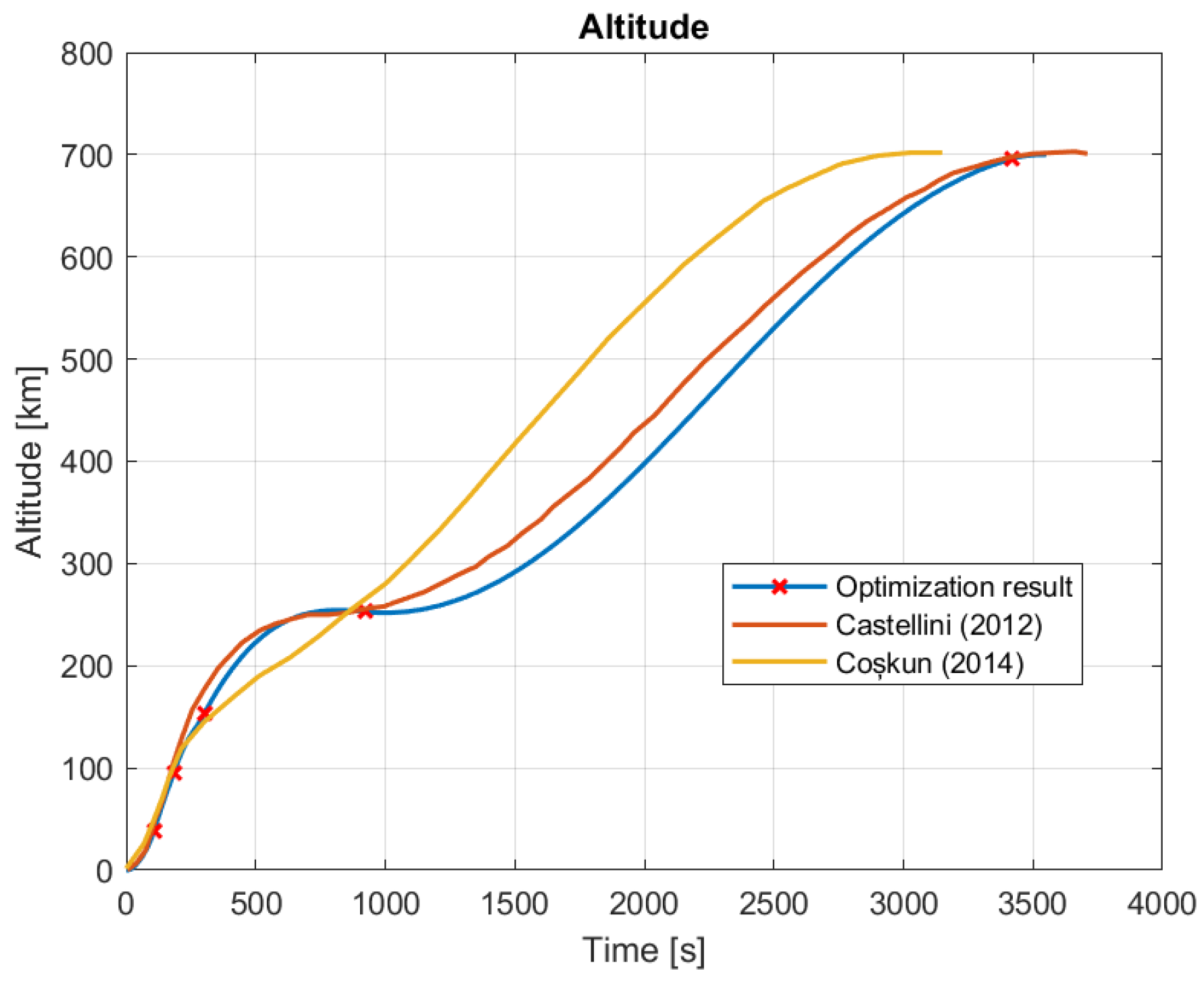
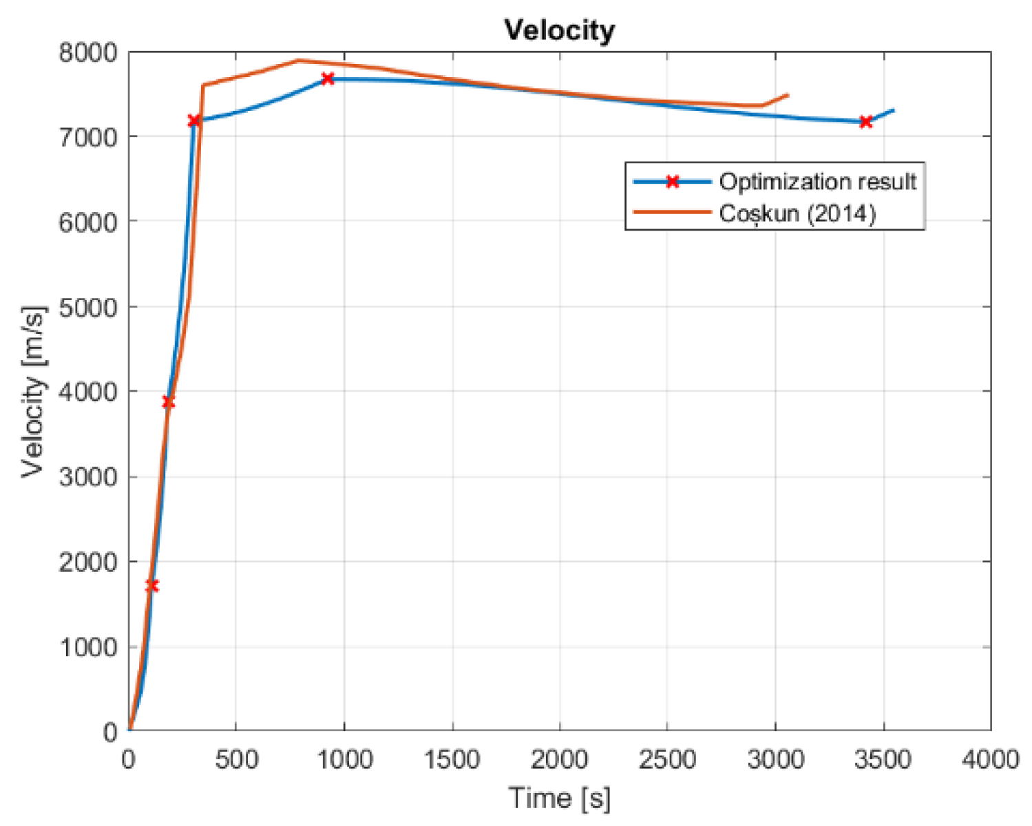
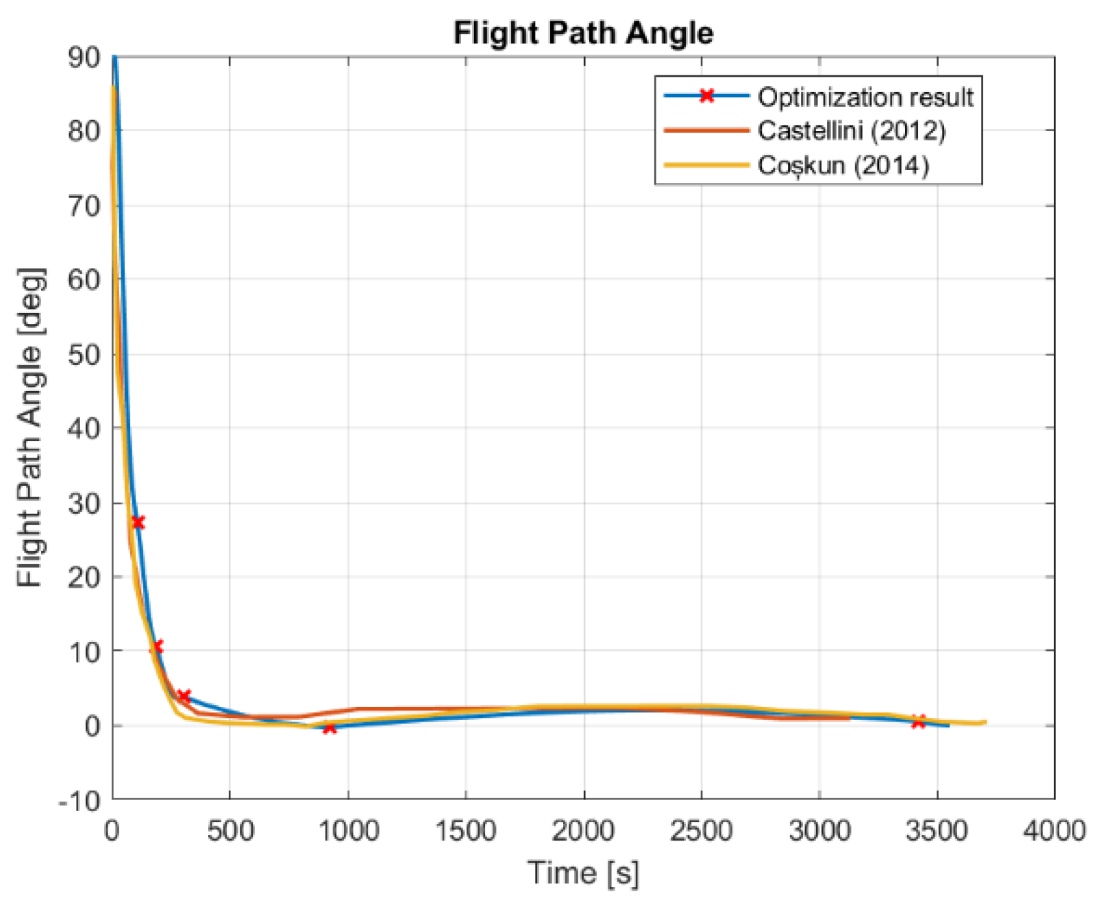
Figure 5, Figure 6 and Figure 7 show how the altitude, the velocity, and the trajectory angle converge to their target values at the end point of the path. That is, the height reaches 700 km, the speed reaches close to the orbital speed of 7.50 km/s, and the trajectory angle reaches approximately 0°, with the payload staying in the target orbit. A comparison of the solutions obtained with the reference data available in the open literature was included [5,35]. A digitalization software was used in order to reproduce the results.

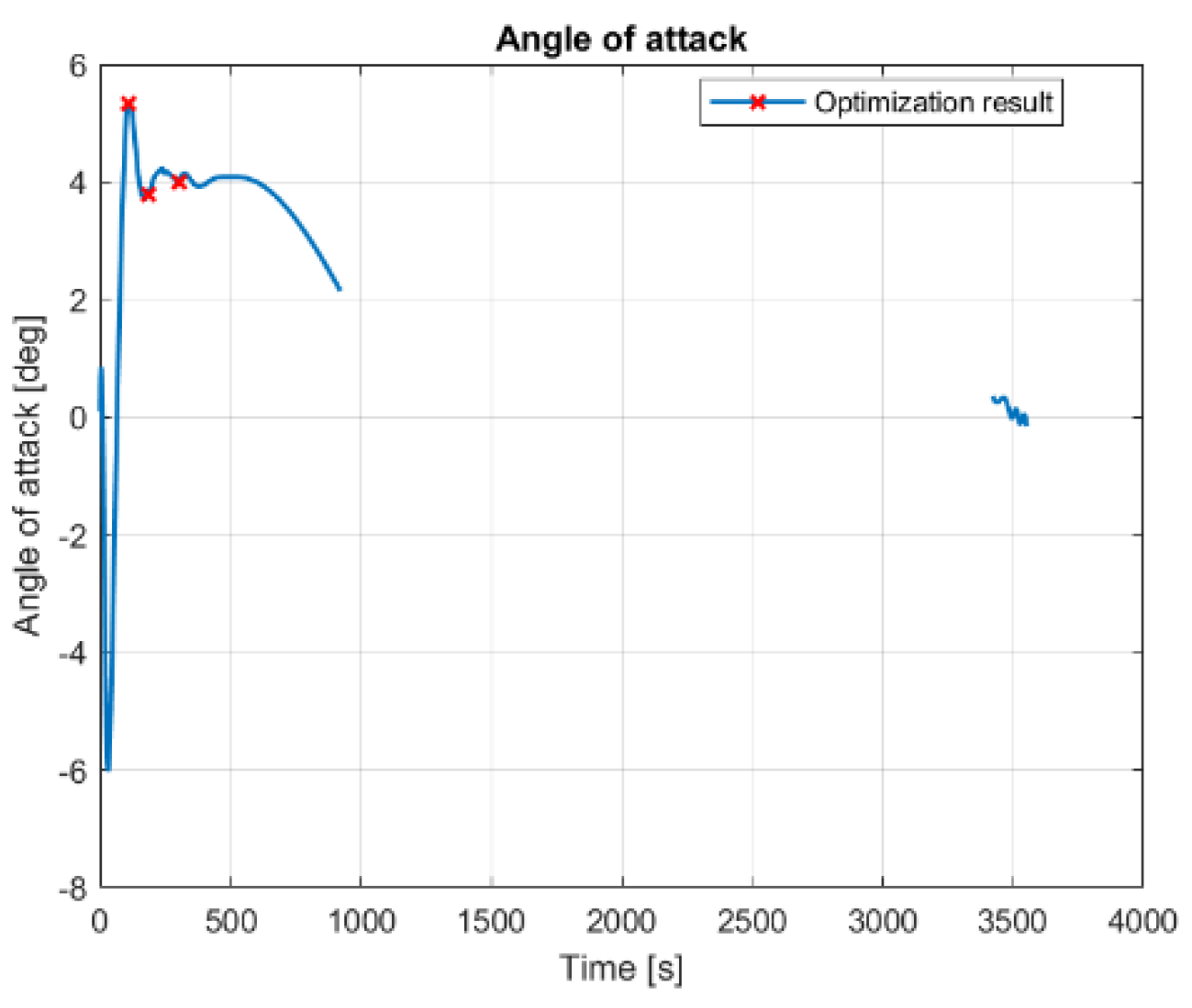
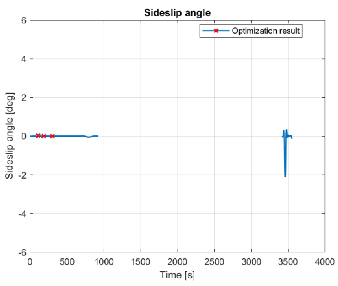
The angles of attack and sideslip, as seen in Figure 8 and Figure 9, on the other hand, range under the selected limitation of the Table 9. To obtain more continuous control variables, 246 extra lineal constraints are implemented to have the value of the control variables within a determinate range of the previous value. In this way, big jumps are prevented but not the smaller ones, which are still present. On the coasting phase, there is no thrust, so the angles are irrelevant and will not be considered.

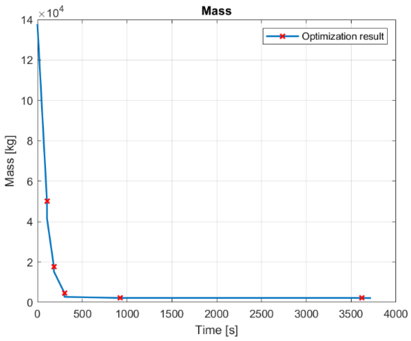
The distribution of the masses with time is, as displayed on Figure 10, not continuous, with low points that correspond to the exhaustion of a stage and its corresponding expulsion.

Table 10. Final orbital elements for the ascend trajectory.

Orbital Element	Simulated Value	Goal Value	Absolute Error	Percentage Error
Altitude (instead of a) [km]	699.99	700	0.01	$8.71 \times {10}^{-5}$%
Eccentricity	0.053	0	0.053	-
Inclination [°]	90.01	90	0.01	0.005%
Longitude of ascending node [°]	6.20	-	-	-
Perigee argument [°]	35.57	-	-	-
True anomaly [°]	180.20	-	-	-

shows the Keplerian elements of the achieved orbit and the target orbit. The differences are small except for the eccentricity that ends in a higher value. An extra maneuver by the spacecraft will have to be considered to circularize the orbit if a circular one is desired. The last three parameters are not specified as objectives and can take an arbitrary value.

Table 11. Maximum values of the constraints in the trajectory.

Constraint	Trajectory Value	Constraint LIMIT
$\alpha$ [°]	6	15 (>100 km)
$\beta$ [°]	0.34	15 (>100 km)
$q$ [Pa]	43,651	55,000
$q\alpha$ [Pa deg]	88,450	230,000
$\dot{q}$ [W/m2]	28,910,000	40,000,000

shows the maximum values that the constraints for the path reach, as well as their limit values. All of them are lower than their respective limits, so the trajectory is structurally and physically viable. The fairing jettisoning should, on the other hand, be done after at least 221 s to be in accordance with the Table 5 constraint. Regarding the available weight for the payload, its value stays at 1431.3 kg, which is a slightly more than 1 kg increase with respect to the real value (a 0.09%). Coșkun [5] arrives to a value of 1488 kg, whereas Castellini [35] arrives to 1403 kg.

4. Conclusions and Future Works

This work addresses the optimization of various parts of a launch vehicle design and its mission. The mass distribution between stages is optimized, both in series and in parallel, thus analyzing the effect of the boosters’ mass on the GLOW. The overall design of a launch vehicle is also optimized by varying the propulsion plant and mass distribution. The aerodynamic, geometric, propulsive, and mass characteristics are studied and defined from the optimization variables. This algorithm is used in the revision of real rockets, obtaining alternative configurations designed for their usual operation.

Finally, the ascent trajectory of a launch vehicle is optimized by means of direct methods, discretizing the trajectory. Structural and physical constraints are taken into account in order to generate a feasible trajectory. The final conditions are specified in order to achieve an injection into a given circular orbit. Trajectory optimization is applied to the trajectory of the Vega rocket, obtaining close results with respect to other modeling algorithms.

The design of a launch vehicle is a broad area, and therefore, there are multiple lines of development to be pursued. Firstly, the scope of use of the design algorithm can be extended by supporting parallel stages, as well as extending the database of available engines.

As for trajectory optimization, direct methods have been used to carry out the process. The implementation of indirect methods, on the other hand, would allow—through the calculation of variations—a more robust and efficient optimization, increasing the mathematical complexity on the contrary. Additionally, the implementation of partial reusability of the rocket could also be considered by specifying a minimum fuel remaining in the first stage at the moment of ignition of the second stage.

Finally, the logical evolution of such programs is to couple the rocket design with trajectory optimization, so aerodynamic and gravity losses can be calculated dynamically, and the design is optimized for a specific mission.

References

- Satellite Database|Union of Concerned Scientists. Available online: https://www.ucsusa.org/resources/satellite-database (accessed on 1 February 2022).
- McConnaughey, P.K.; Femminineo, M.G.; Koelfgen, S.J.; Lepsch, R.A.; Ryan, R.M.; Taylor, S.A. Launch Propulsion Systems Roadmap. Technol. Area 2012, 1, 78−92. [Google Scholar]
- Tewari, A. Atmospheric and Space Flight Dynamics: Modeling and Simulation with MATLAB® and Simulink®; Springer Science & Business Media: Berlin/Heidelberg, Germany, 2007. [Google Scholar]
- Tewari, A. Advanced Control of Aircraft, Spacecraft, and Rockets, Aerospace Series; Wiley: Chichester, UK, 2011. [Google Scholar]
- Coşkun, E.C. Multistage Launch Vehicle Design with Thrust Profile and Trajectory Optimization. Ph.D. Dissertation, Middle East Technical University, Ankara, Turkey, 2014. [Google Scholar] [CrossRef]
- Conway, B.A. (Ed.) Spacecraft Trajectory Optimization; Cambridge University Press: Cambridge, UK, 2010; Volume 29. [Google Scholar]
- Rao, A. A Survey of Numerical Methods for Optimal Control. Adv. Astronaut. Sci. 2010, 135, 1. [Google Scholar]
- Betts, J.T. Survey of Numerical Methods for Trajectory Optimization. J. Guid. Control. Dyn. 1998, 21, 193–207. [Google Scholar] [CrossRef]
- Gath, P.F.; Well, K.H.; Mehlem, K. Initial Guess Generation for Rocket Ascent Trajectory Optimization Using Indirect Methods. J. Spacecr. Rocket. 2002, 39, 515–521. [Google Scholar] [CrossRef]
- Pontani, M. Particle swarm optimization of ascent trajectories of multistage launch vehicles. Acta Astronaut. 2014, 94, 852–864. [Google Scholar] [CrossRef]
- Filatyev, A.S.; Yanova, O.V. Through optimization of branching injection trajectories by the Pontryagin maximum principle using stochasticmodels. Acta Astronaut. 2011, 68, 1042–1050. [Google Scholar] [CrossRef]
- Brusch, R.G. A nonlinear programming approach to space shuttle trajectory optimization. J. Optim. Theory Appl. 1974, 13, 94–118. [Google Scholar] [CrossRef]
- Jänsch, C.; Schnepper, K.; Well, K.H. Multi-phase trajectory optimization methods with applications to hypersonic vehicles. In Applied Mathematics in Aerospace Science and Engineering. Mathematical Concepts and Methods in Science and Engineering; Miele, A., Salvetti, A., Eds.; Springer: Boston, MA, USA, 1994; Volume 44. [Google Scholar] [CrossRef]
- Bollino, K.P.; Bollino, K.P. High-Fidelity Real-Time Trajectory Optimization for Reusable Launch Vehicles; Naval Postgraduate School Monterey: Monterey, CA, USA, 2006. [Google Scholar]
- Zotes, F.A.; Penas, M.S. Multi-criteria genetic optimisation of the manoeuvres of a two-stage launcher. Inf. Sci. 2010, 180, 896–910. [Google Scholar] [CrossRef]
- Nguyen, H. Optimal Ascent Trajectories of the Horizontal Takeoff Single-Stage and Two-Stage-to-Orbit Launchers. In Proceedings of the Navigation and Control Conference; American Institute of Aeronautics and Astronautics: New Orleans, LA, USA, 1991. [Google Scholar]
- Yanova, O.; Filatyev, A. ASTER program package for the thorough trajectory optimization. In Proceedings of the AIAA Guidance, Navigation, and Control Conference and Exhibit, American Institute of Aeronautics and Astronautics, Montreal, QC, Canada, 6–9 August 2001. [Google Scholar] [CrossRef]
- Handbook of Space Technology; Ley, W.; Wittmann, K.; Hallmann, W. (Eds.) Wiley: Chichester, UK, 2009; ISBN 978-1-60086-701-9. [Google Scholar]
- Sarigul-Klijn, M.; Sarigul-Klijn, N. Flight mechanics of manned sub-orbital reusable launch vehicles with recommendations for launch and recovery. In Proceedings of the 41st Aerospace Sciences Meeting and Exhibit, Aerospace Sciences Meetings, American Institute of Aeronautics and Astronautics, Reno, NV, USA, 6–9 January 2003. [Google Scholar] [CrossRef] [Green Version]
- Wertz, J.R.; Larson, W.J. (Eds.) Space Mission Analysis and Design, 3rd ed.; Space Technology Library, Microcosm; Kluwer: El Segundo, CA, USA; Dordrecht, The Netherlands; Boston, UK, 1999. [Google Scholar]
- Haidn, O.J. Advanced Rocket Engines. In Advances on Propulsion Technology for High-Speed Aircraft; Educational Notes RTO-EN-AVT-150, Paper 6; RTO: Neuilly-sur-Seine, France, 2008; pp. 6-1–6-40. [Google Scholar]
- Braeunig, R.A. Basics of Space Flight: Rocket Propellants. Available online: http://www.braeunig.us/space/propel.htm (accessed on 8 December 2021).
- Sutton, G.P.; Biblarz, O. Rocket Propulsion Elements, 8th ed.; Wiley: Hoboken, NJ, USA, 2010. [Google Scholar]
- Wade, M. Encyclopedia Astronautica. 2019. Available online: http://www.astronautix.com/ (accessed on 8 December 2021).
- Meng, Z.; Li, G.; Wang, X.; Sait, S.M.; Yıldız, A.R. A comparative study of metaheuristic algorithms for reliability-based design optimization problems. Arch. Comput. Methods Eng. 2021, 28, 1853–1869. [Google Scholar] [CrossRef]
- Akin, D.A. Mass Estimating Relations; University of Maryland: College Park, MD, USA, 2016. [Google Scholar]
- Mandell, G.K.; Caporaso, G.J.; Bengen, W.P. Topics in Advanced Model Rocketry; MIT Press: Cambridge, MA, USA, 1990. [Google Scholar]
- Hoerner, S.F. Fluid-Dynamic Drag: Practical Information on Aerodynamic Drag and Hydrodynamic Resistance; Hoerner Fluid Dynamics: Bakersfield, CA, USA, 1992. [Google Scholar]
- Fleeman, E.L. Tactical Missile Design, AIAA Education Series; American Institute of Aeronautics and Astronautics: Reston, VA, USA, 2001. [Google Scholar]
- Torczon, V. On the Convergence of Pattern Search Algorithms. SIAM J. Optim. 1997, 7, 1–25. [Google Scholar] [CrossRef]
- Civek-Coskun, E.; Ozgoren, K. A Generalized Staging Optimization Program for Space Launch Vehicles. In Proceedings of the 2013 6th International Conference on Recent Advances in Space Technologies (RAST); IEEE: Istanbul, Turkey, 2013; pp. 857–862. [Google Scholar]
- Koelle, D.E. Handbook of Cost Engineering for Space Transportation Systems with TRANSCOST 8.2: Statistical-Analytical Model for Cost Estimation and Economical Optimization of Launch Vehicles; TransCostSystems: Amiens, France, 2013. [Google Scholar]
- Isakowitz, S.J.; Hopkins, J.P.; Hopkins, J.B. International Reference Guide to Space Launch Systems, 4th ed.; American Institute of Aeronautics and Astronautics: Reston, VA, USA, 2004. [Google Scholar]
- Rockets—Spaceflight101. Rockets. 2022. Available online: https://spaceflight101.com/spacerockets/ (accessed on 1 February 2022).
- Castellini, F. Multidisciplinary Design Optimization for Expendable Launch Vehicles; Politecnico di Milano: Milan, Italy, 2012. [Google Scholar]
- Ritter, P.; Lyne, J.E. Design and selection process for optimized heavy lift launch vehicles. In Proceedings of the 48th AIAA/ASME/SAE/ASEE Joint Propulsion Conference & Exhibit, American Institute of Aeronautics and Astronautics, Atlanta, Georgia, 30 July–1 August 2012. [Google Scholar] [CrossRef]
- Cremaschi, F. Trajectory optimization for launchers and re-entry vehicles. In Modeling and Optimization in Space Engineering, 127th ed.; Fasano, G., Pintér, J.D., Eds.; Springer (Springer Optimization and Its Applications): Berlin/Heidelberg, Germany, 2012; pp. 159–185. [Google Scholar]
- Federici, L.; Zavoli, A.; Colasurdo, G.; Mancini, L.; Neri, A. Integrated Optimization of Ascent Trajectory and SRM Design of Multistage Launch Vehicles; Cornell University: Ithaca, NY, USA, 2019. [Google Scholar] [CrossRef]
Figure 1.
Diagram of a launch vehicle with parallel stages [31].
Figure 2.
Design algorithm diagram.
Figure 3.
Trajectory optimization algorithm diagram.
Figure 4.
Optimization of the GLOW in function of the boosters’ mass.
Figure 5.
Altitude in the optimized trajectory. The red marks indicate the staging or coasting phase.
Figure 6.
Velocity in the optimized trajectory. The red marks indicate the staging or coasting phase.
Figure 7.
Flight path angle in the optimized trajectory. The red marks indicate the staging or coasting phase.
Figure 8.
Angle of attack in the optimized trajectory. The red marks indicate the staging or coasting phase.
Figure 9.
Sideslip angle in the optimized trajectory. The red marks indicate the staging or coasting phase.
Figure 10.
Mass evolution in the optimized trajectory. The red marks indicate the staging or coasting phase.