Assessment of Radiative Heating for Hypersonic Earth Reentry Using Nongray Step Models

Abstract

Accurate prediction of the aerothermal environment is of great significance to space exploration and return missions. The canonical Fire II trajectory points are simulated to investigate the radiative transfer in the shock layer for Earth reentry at hypervelocity above 10 km/s using a developed radiation–flowfield uncoupling method. The thermochemical nonequilibrium flow is solved by an in-house PHAROS Navier–Stokes code, while the nongray radiation is integrated by the tangent slab approximation, respectively, combined with the two-, five-, and eight-step models. For the convective heating, the present results agree well with the data of Anderson’s relation. For the radiative heating, the two-step model predicts the closest values with the results of Tauber and Sutton’s relationship, while the five- and eight-step models predict far greater. The three-step models all present the same order of magnitude of radiative heating of 1 MW/m² and show a consistent tendency with the engineering estimation. The Planck-mean absorption coefficient is calculated to show the radiative transfer significantly occurs in the shock layer. By performing the steady simulation at each flight trajectory point, the present algorithm using a nongray step model with moderate efficiency and reasonable accuracy is promising to solve the real-time problem in engineering for predicting both convective and radiative heating to the atmospheric reentry vehicle in the future.

1. Introduction

Today, many countries are energetically developing planetary exploration and subsequent return projects [1]. The mission spacecraft, usually with a blunt nose, must undergo the harsh thermal environment at hypervelocity even greater than 10 km/s for Earth atmosphere reentry [2]. In this situation, the strong bow shock wave around the reentry forebody can stimulate an extremely high temperature with an order of magnitude of 10,000 K and very complicated thermochemical nonequilibrium phenomena including the high excitations of vibrational and electronic energy modes, dissociation, and ionization reactions of molecules and atoms of air species [3,4,5]. Except for the convective and chemical diffusive heating, radiative heat transfer could be a considerable or even dominated contributor to the total aerodynamic heating [6].

In fact, the occurrence of air radiation is not only one simple additional mode of heat transfer but also has important impacts on the flow characteristics of the shock layer [7]. On one hand, the radiative energy emission and absorption make the flowfield nonadiabatic and lead to the radiation cooling effect [8], which results in a lower temperature, higher density, and subsequently thinner shock layer. On the other hand, the thermochemical reactions and radiation of air species may overlap in some concerned flight regimes. The radiation limits the chemical reaction processes of air species, whereas the air thermodynamic states and composition, in turn, directly affect the level of radiance. The radiation–flowfield coupling should be evaluated [9]. Therefore, in engineering, the thermal protection system design of the entry vehicle requires the accurate aerothermal analysis of the hypersonic thermochemical nonequilibrium flowfield including radiation to ensure safe entry [10,11,12].

However, until now, the solution of radiation in the hypersonic shock layer has not been an easy task [13], even for the uncoupled radiation calculation only [14]. First, although the scattering could be neglected, the absorption and emission must be accounted for in the air radiation in the hypersonic shock layer. The radiation properties of air, which are emission and absorption coefficients, always vary dramatically with the frequency ranging from zero to infinity [15]. The accurate calculation of the air absorption coefficients requires a very large number of frequency points with an order of one million, which is undoubtedly time-consuming and even unaffordable [16]. Second, the radiative transfer depends on the multi-dimensions of space, angle, and frequency. The algorithm for solving the radiative transfer equation (RTE) has to simultaneously account for the spatial, angular, and frequency discretizations, which makes the radiation computation difficult and inefficient [17]. Facing the foregoing barriers, it is necessary to employ the reduced models to calculate the air radiation property and energy transportation for the aerodynamic heating to reentry vehicle [18].

The step model is an efficient method to calculate the air radiation property with moderate accuracy [19]. It divides the whole frequency space into several spectral intervals even including atomic lines in which the radiative absorption coefficient is equivalent to a constant [20]. Although the step model appears to be coarser than the line-by-line or multi-band models, it usually can predict the reasonable radiative flux of the hypersonic vehicle [21]. For solving radiative transfer, there have been various numerical methods, such as the tangent slab (TS) approximation [22], the spherical harmonics method [23], the ray-tracing method [24], the finite volume method [25], the discrete ordinates method [26], and Monte Carlo method [27]. Each method has both advantages and disadvantages either in prediction accuracy or in computation efficiency [28]. Among these methods, TS has seemed to be the most frequently used method for both coupled and uncoupled flowfield-radiation simulations for decades [2]. TS originates from the one-dimensional analytical integrated solution of RTE for the participating medium between two infinite parallel plates with the radiation variations only along the normal direction of the plate [22]. Since the shock layer flow and thermodynamic properties mainly vary in the direction normal to the surface of the blunt-nosed reentry vehicle, TS is a good approximation to model the radiation energy-transportation [29]. Practically, researchers usually use the body-normal grid lines for convenient TS calculation [2]. Hartung et al. used TS to evaluate the characteristics of the shock wave precursor ahead of the hypervelocity entry vehicle including the radiative effects [30]. Wright et al. found that TS could over-predict the value of the stagnation radiative heat flux by a minimum of 20% for the Titan aerocapture case [31]. Johnston et al. used TS combined with a viscous shock layer flowfield model to account for the radiation–flowfield coupling and showed that the coupled simulation reduced the radiative heating by about 30%, while the convective heating decreased slightly [32]. Bauman et al. coupled a reacting flow model and a surface ablation model with TS to develop a two-way loose-coupling procedure for simulating the hypersonic flows with radiation and ablation [33]. Johnston and Brandis employed TS to calculate the radiative heating and identified the radiation as a major contributor to afterbody heating for Earth entry at velocities above 10 km/s. They also showed that TS overestimates the afterbody radiative heat transfer by as much as 50% [34]. Generally, although TS has some deficiencies and researchers have also proposed a non-tangent-slab procedure, TS is still very worthy of being considered as a first choice to solve RTE coupled or uncoupled with flowfield solver to predict the radiative heating for Earth reentry at hypervelocity, especially to obtain a conservative estimation of the aerodynamic heating in the engineering initial design with moderate accuracy and computation efficiency.

In fact, there have been many engineering empirical relations to quickly predict both the wall convective and radiative heat fluxes of the Earth entry capsule [35]. Most methods have been too coarse for the modern design of Earth reentry capsule which can only give the value of heat transfer at the stagnation point but has no ability to present the distribution characteristics of aerodynamic heating and some key physical variables of interest in the shock layer, such as electrons number density and radiation absorption coefficient. However, the accurate radiation–flowfield coupling simulation is time-consuming and even unaffordable for the initial thermal protection system design of reentry vehicles [16]. Hence, it is more rational and practical in engineering to choose an uncoupled radiation–flowfield procedure, in which the radiation is calculated only once based on the flow simulation results [36].

Gupta et al. used a viscous shock-layer code and aerotherm radiation code with nonequilibrium and equilibrium chemistry to estimate the convective and radiative heating of the Fire II vehicle, but the calculations were limited to the stagnation region [37]. Olynick et al. developed a nonequilibrium, axisymmetric flow solver coupled with a radiation GIANTS/NOVAR code to obtain values of the stagnation radiation intensity in the 0.2 and 6.2 eV and the total aerodynamic heating over the entire Fire II vehicle, which provided the better predictions than previously numerical simulations [38]. Palmer et al. incorporated the NEQAIR line-by-line radiation code into the DPLR flow solver to investigate the effects of fluid dynamics/radiation coupling by comparing coupled and uncoupled results, and they found that the greatest coupling effect of Fire II occurred at the 1643 s trajectory point [39]. Soucasse et al. implemented a hybrid statistical narrow band (HSNB) model with a two-temperature nonequilibrium model to calculate the 1D stagnation line radiative transfer. The HSNB model could reproduce the line-by-line results with an accuracy of better than 5% and a computational time speed up about two orders of magnitude [40]. Bonin and Mundt developed a full three-dimensional photon Monte Carlo radiative transport solver to study arbitrary thermal radiation within equilibrium and nonequilibrium hypersonic flows, the code of which was line-by-line accurate but time-consuming [41]. Although great progress has been made to predict radiative transfer in hypersonic nonequilibrium flow for atmospheric entry over decades, the too sophisticated methods developed with high accuracy are always of much heavy computational burden and even unaffordable, such as the line-by-line and narrow-band radiation models, especially for multi-dimensional coupling simulation. Therefore, there is still a practical demand for developing the reduced models with moderate time efficiency and reasonable accuracy to predict both radiative heating and radiation characteristics in flowfield for the thermal protection design of Earth reentry vehicles in engineering applications.

For solving the above-mentioned problems, the first objective of this paper is to develop an uncoupled radiation–flowfield algorithm for predicting the aerothermal environment of Earth reentry vehicles at hypervelocities above 10 km/s, which consists of the tangent slab approximation, the nongray step model, and a Navier–Stokes solver including the thermochemical nonequilibrium effects. The detailed physical models and numerical schemes are presented in Section 2. Another objective is to evaluate the performance of the radiation–flowfield uncoupling procedure by analyzing the canonical reentry trajectory cases of Fire II capsule, especially focusing on the aerodynamic heating and the radiation characteristics in the shock layer. The convective and radiative heat fluxes at the stagnation point are also estimated throughout the trajectory, respectively, using the Anderson and Tauber and Sutton relations. A comparison between the present results and those of engineering methods and previous studies is thoroughly presented and discussed in Section 3. The final conclusions are drawn in Section 4.

2. Physical Models and Numerical Methods

2.1. Flow Governing Equations with Thermochemical Nonequilibrium Models

The hypersonic Earth reentry flow is governed by the Navier–Stokes equations with the two-temperature model including the thermochemical nonequilibrium effects in the conservative forms. It assumes that the air is a multi-gas mixture and for all the composite species, the translational and rotational energy modes are in equilibrium in one translational-rotational temperature, T_tr, and the vibrational, electronic, and electron energies are uniformly described by one vibrational-electronic temperature, T_ve [42]. In this manner, the mass, momentum, and energy conservation equations of the hypersonic nonequilibrium flow can be expressed as follows [3]:

$$\frac{\partial {\rho }_s}{\partial t}+\frac{\partial {\rho }_s{u}_j}{\partial x_j}=-\frac{\partial J_{s,j}}{\partial x_j}+{\omega }_s,s=1,2,\cdots ,N_s$$

(1)

$$\frac{\partial \rho u_i}{\partial t}+\frac{\partial \rho u_i{u}_j}{\partial x_j}=-\frac{\partial p}{\partial x_i}+\frac{\partial }{\partial x_j}\left[\mu \left(\frac{\partial u_i}{\partial x_j}+\frac{\partial u_j}{\partial x_i}\right)-\frac{2}{3}\mu \frac{\partial u_k}{\partial x_k}{\delta }_{ij}\right]$$

(2)

$$\frac{\partial \rho e}{\partial t}+\frac{\partial \rho h{u}_j}{\partial x_j}=\frac{\partial {\tau }_{ij}{u}_i}{\partial x_j}-\frac{\partial q_j}{\partial x_j}-\frac{\partial }{\partial x_j}\left({\displaystyle \sum _{s=1}^{N_s}{J}_{s,j}{h}_s}\right)+{\omega }_r$$

(3)

$$\frac{\partial \rho e_{ve}}{\partial t}+\frac{\partial \rho e_{ve}{u}_j}{\partial x_j}=-\frac{\partial q_{ve,j}}{\partial x_j}-\frac{\partial }{\partial x_j}\left({\displaystyle \sum _{s=1}^{N_s}{J}_{s,j}{h}_{ve,s}}\right)+{\omega }_{ve}+{\omega }_r$$

(4)

where t is the time, x_i is the ordinate variable in the i direction, N_s is the total number of the air species, ρ_s and ρ are the species density and total density, u_i is the flow velocity component in the i direction, p is the pressure, τ_ij is the viscous stress tensor, e and e_ve are the total energy and vibrational-electronic energy, h is the total enthalpy, q_j and q_ve,j are the total heat flux and vibrational-electronic heat flux, h_s and h_ve,s are the enthalpy and vibrational-electronic enthalpy of the species s, J_s,j is the mass diffusion flux of the species s in the j direction, ω_s is the mass production rate of the species s per unit volume, ω_ve is the vibrational-electronic energy source term, and ω_r is the radiative source term. The state equation of the air follows:

$$p={\displaystyle \sum _{s=1}^{N_s-1}{\rho }_s{R}_s{T}_{tr}}+{\rho }_e{R}_e{T}_{ve}$$

(5)

where the subscript “e” represents the electron.

In the present study, the thermodynamic properties of all the species are calculated using analytical relations of the translational, rotational, and electronic excitation energy modes based on the Born–Oppenheimer approximation [43]. The transport properties of the air mixture including the dynamic viscosity, thermal conductivity, and species diffusion coefficients are calculated via the extension of Yos’ formula with the collision integrals [44].

The mass rate of production of species s is expressed as follows [45]:

$${\omega }_s=M_s{\displaystyle \sum _{r=1}^{N_r}\left({\nu }_{r,s}^b-{\nu }_{r,s}^f\right)\left[k_{f,r}{\displaystyle \prod _{j=1}^{N_s}{\left(\frac{{\rho }_j}{M_j}\right)}^{{\nu }_{r,j}^f}}-k_{b,r}{\displaystyle \prod _{j=1}^{N_s}{\left(\frac{{\rho }_j}{M_j}\right)}^{{\nu }_{r,j}^b}}\right]}$$

(6)

where N_r is the total number of chemical reactions, M_s is the molecular mass per mole of species s, ν^f_r,s and ν^b_r,s are the forward and backward reaction stoichiometric coefficients of species s of the r-th reaction, k_f,r and k_b,r are the forward and backward reaction rate coefficients of the r-th reaction, respectively. For each chemical reaction, the forward reaction rate coefficient is calculated using the Arrhenius formula [46], while the backward reaction rate coefficient is obtained from the corresponding forward reaction rate coefficient divided by the equilibrium constant, which is computed using the temperature fitting expression [44].

The vibrational-electronic energy source term ω_ve is modeled in the expression proposed by Gnoffo et al. [46], in which the translational-vibrational energy exchange part is calculated by the Landau–Teller model [47], and the relaxation time is calculated by the Millikan–White expression [48] with Park’s high-temperature correction [49]. For the present uncoupled radiation–flowfield simulation, the radiative source term ω_r is neglected.

2.2. Flowfield Solver

The Navier–Stokes equations with thermochemical models are solved using an in-house CFD code PHAROS (Parallel Hypersonic Aerothermodynamics and Radiation Optimized Solver) [50]. PHAROS is a parallel multi-block finite volume solver, in which the inviscid fluxes are computed by the modified Steger–Warming flux vector splitting scheme [51] using MUSCL extrapolation [52] with minmod limiters for high order accuracy and stability. The viscous fluxes are discretized in the second central difference. A line relaxation approach is employed for the time marching [53]. PHAROS has been used to solve many types of hypersonic thermochemical nonequilibrium flowfields [3,5,6,54]. More information on PHAROS can be found in Ref. [50].

2.3. Step Models for Radiation Properties

Based on recognizing the variation characteristics of the self-absorption property of air radiation with wavelength, the step model selects some demarcation wavelength points and divides the infinite spectrum into several consecutive spectral regions, such as vacuum ultraviolet and visible bands. In each spectral band, the volatile radiation absorption coefficients are averaged into a constant Planck-mean value, which makes the total radiation a sum of the contributions of all the step regions. The absorption coefficient in the spectral region of each step depends on the temperature, density, and air composition parameters [20]. It has been shown that the step model can well account for the important effects of shock-layer nongray self-absorption and radiative cooling on radiative heat transfer [19]. Additionally, compared to line-by-line calculation, the step model is a reasonable simplification and can reduce the computational time obviously. Therefore, the step model is selected for the present study. In this paper, the radiation absorption coefficients of the high-temperature gas mixture of air are calculated via the two-step, five-step, and eight-step nongray models [55], respectively, for the purpose of comparative study. The two-step and five-step models are developed based on the high-temperature atomic nitrogen mainly accounting for the air radiance at temperatures above 8000–10,000 K, while the eight-step model includes both the atomic and molecular emission absorption of the high-temperature air [56]. The wavelength regions of the three foregoing step models are listed in

Table 1. Spectral regions of two-, five-, and eight-step models.

Model	Step No.	Wavelength (Å)	Spectral Band
Two-step	1	0–1100	VUV (vacuum ultraviolet)
	2	1100–∞	Visible
Five-step	1	620–1100	VUV continuum
	2	1100–1300	VUV continuum
	3	1300–1570	VUV lines
	4	1570–7870	Visible
	5	7870–9552	IR (infrared) lines
Eight-step	1	400–852	VUV continuum
	2	852–911	VUV continuum
	3	911–1020	VUV continuum
	4	1020–1130	VUV continuum
	5	1130–1801	Continuum + line wings
	6	1130–1801	Line “centers”
	7	1801–4000	Visible
	8	4000–∞	Visible + infrared

. The specific formulas and parameters of the three-step models are given in Appendix A.

2.4. Tangent Slab (TS) Approach for RTE

Neglecting the gas scattering effect, the high-temperature air radiation process in the hypersonic reentry shock layer is described via the radiative transfer equation (RTE) as follows [57]:

$$B_j\frac{\partial I_{\nu }\left(x,B\right)}{\partial x_j}={\kappa }_{\nu }\left(x\right)\left[I_{b\nu }\left(x\right)-I_{\nu }\left(x,B\right)\right]$$

(7)

where x represents the spatial position vector, ν is the radiation frequency, I_ν and I_bν is the spectral radiative intensity and blackbody radiative intensity at frequency ν, respectively, B_j is the j-th component of unit vector B in the transmission direction of I_ν, and κ_ν is the spectral absorption coefficient at x.

TS approximates the hypersonic shock layer around the reentry blunt body as an infinite slab with physical variables only changing in the perpendicular direction to the body surface. Hence, there is an integrated solution for RTE as follows [22]:

$$q_{rw}={\epsilon }_w\left(J_w-\sigma T_w^4\right)$$

(8)

and

$$J_w=2\pi {\displaystyle {\int }_0^{\infty }\left[I_{\nu }\left({\tau }_{\nu \delta }\right)E_3\left({\tau }_{\nu \delta }-{\tau }_{\nu w}\right)+{\displaystyle {\int }_{{\tau }_{\nu w}}^{{\tau }_{\nu \delta }}{I}_{b\nu }\left(t\right)E_2\left(t-{\tau }_{\nu w}\right)\mathrm{d}t}\right]\mathrm{d}\nu }$$

(9)

where τ_ν is the optical thickness at frequency ν perpendicular to the body surface (τ_ν = 0 at body surface), the subscript “δ” and “w” represent the outer edge of the shock layer and the wall, respectively; t is a dummy variable of integration, and ε_w and T_w are the wall emissivity and temperature, respectively. E_n is the integro-exponential function of order n as follows:

$$E_n\left(t\right)\equiv {\displaystyle {\int }_0^1{s}^{n-2}{e}^{-t/s}\mathrm{d}s}$$

(10)

According to step models in Section 2.3, the integration (9) can be written as:

$$J_w=2\pi {\displaystyle \sum _m\left\{E_3\left({\tau }_{m\delta }-{\tau }_{mw}\right){\displaystyle {\int }_m{I}_{\nu }\left({\tau }_{\nu \delta }\right)\mathrm{d}\nu }+{\displaystyle {\int }_{{\tau }_{mw}}^{{\tau }_{m\delta }}\left[{\displaystyle {\int }_m{I}_{b\nu }\left(t\right)\mathrm{d}\nu }\right]\times E_2\left(t-{\tau }_{mw}\right)\mathrm{d}t}\right\}}$$

(11)

where m is the index of the step region. In this paper, the integral with respect to optical thickness in Equation (11) is calculated using the trapezoidal method to perform TS procedures.

2.5. Radiation–Flowfield Uncoupling Algorithm

For radiation–flowfield coupling simulation, TS approximation with a nongray step model should do the upward and downward integrals of radiative heat flux divergence along the ray line normal to the wall for computing the radiative source term ω_r in Equation (4) [22]. Assuming a two-dimensional problem is solved, the mesh has a total number of grid nodes of N_ξ × N_η, where N_ξ is the discretized number parallel to the wall and N_η is the discretized number normal to the wall. Thus, the coupling simulation should need about N_ξ × N_η × M × N_η calculations in one radiation iteration, for which the last product factor N_η is due to the numerical integration of radiative heat flux divergence and M is the number of radiation step regions.

A radiation–flowfield uncoupling algorithm is proposed in the present study, in which the hypersonic reentry flow with nonequilibrium chemistry is first solved by PHAROS in Section 2.2, and then the radiation transfer is calculated only once based on the convergent flowfield by the nongray step model in Section 2.3 and TS approximation in Section 2.4. It only needs N_ξ × M × N_η calculations for radiation solution in total. Therefore, in one iteration, the number of calculations for coupled radiation simulation is far greater with an order of magnitude of O(N_η) than that of the present uncoupled algorithm. Particularly, the present scheme only needs to compute radiation one time in total, while the coupled simulation has to update the radiation in each step over the whole computational process. Even for the loosely coupled manner, it still requires a considerable computational cost, in which the radiation is updated one time after a certain number of flow iterations. Therefore, the present method is more time-efficient. Additionally, the present algorithm can provide more radiation information including the radiative heating to the whole surface of the reentry vehicle and the absorption properties distributed in the flowfield, but the engineering methods certainly cannot make it, that will be seen later in Section 3.4.

3. Results and Discussion

Fire II was a scaled-down Apollo-shaped capsule launched in 1965 with the calorimeter instrumentation to obtain reentry heating at hyperbolic velocities. In the reentry phase, Fire II jettisoned two nonablating heat shields in sequence at selected trajectory points, thereby with various vehicle nose radiuses. The Fire II flight experiment has become a benchmark for investigating the aerothermal environment for hypersonic Earth entry. Six trajectory points of Fire II have been simulated in the present study with the flight conditions listed in

Table 2. Fire II flight conditions for the present study.

Time (s)	H (km)	V∞ (km/s)	Ma	RN (m)	ρ∞ (kg/m3)	T∞ (K)	Tw (K)
1634	76.42	11.36	40.58	0.935	3.72 × 10−5	195	615
1636	71.02	11.31	38.94	0.935	8.57 × 10−5	210	810
1637	67.05	11.25	37.17	0.935	1.47 × 10−4	228	1030
1640	59.62	10.97	34.34	0.935	3.86 × 10−4	254	1560
1643	53.04	10.48	31.47	0.805	7.80 × 10−4	276	640
1645	48.37	9.83	29.05	0.805	1.32 × 10−3	285	1520

, where H is the flight altitude, V_∞ and Ma are the flight velocity and Mach number, R_N is the vehicle nose radius, ρ_∞ and T_∞ are the freestream density and temperature, and T_w is the wall temperature. For each case in Table 2, the time of flow over the vehicle, R_N/V_∞, is of an order of magnitude around 10⁻⁴ s, but the time scale of entry down in the altitude is around 0.5 s. The latter is far greater than the former, which means a steady flowfield establishes very quickly. Therefore, we can use the present algorithm to perform steady simulation for each case to fulfill the real-time prediction throughout the Fire II trajectory. Only the Fire II forebody is considered in this paper, the axisymmetric geometry and grids of which are shown in Figure 1. The computational mesh has the dimensions of 153 × 128 (axial × radial) for every case and the spacing of the first grid layer perpendicular to the wall can ensure the cell Reynolds number with an order of magnitude of one in order to predict the reliable aerodynamic heating [58]. The noncatalytic wall condition is used and the wall emissivity is uniformly set to be one.

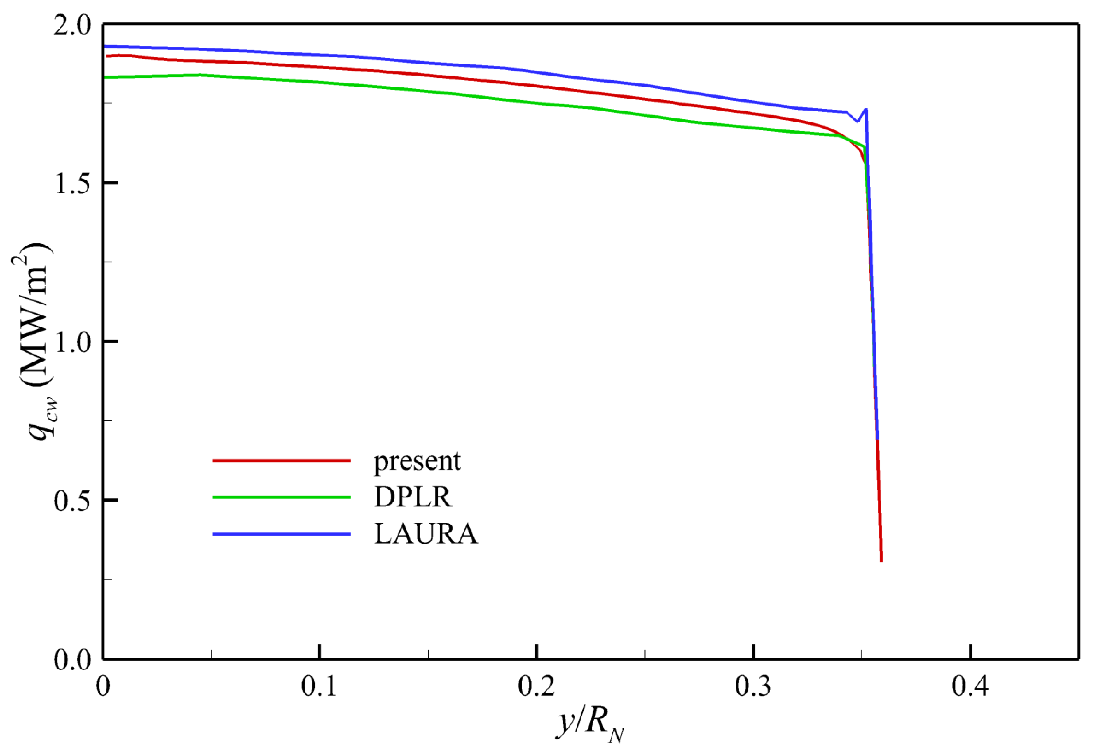
3.1. Convective Heating

Figure 2 compares the present CFD results of convective heat transfer at the stagnation point with those data calculated by Anderson’s engineering relationship [35], Gupta et al. [37], and Olynick et al. [38]. Anderson’s relationship is expressed as follows:

$$q_{cw,stag}=1.83\times {10}^{-4}\sqrt{\frac{{\rho }_{\infty }}{R_N}}\times \left(1-\frac{H_w}{H_e}\right)\times V_{\infty }^3({\mathrm{W}/\mathrm{m}}^2)$$

(12)

where R_N is the vehicle nose radius; ρ_∞ and V_∞ are the freestream density and velocity; H_w and H_e are the enthalpies at the wall and the outer edge of the boundary layer, which can be evaluated by using the wall temperature T_w and freestream total temperature T₀, respectively. T₀ can be calculated by the freestream temperature T_∞ and Mach number Ma. R_N, ρ_∞, V_∞, T_w, T_∞, and Ma are all listed in Table 2.

The present results agree well with the other three sets of data both in the magnitude of value at each trajectory point and the total variation tendency with time, which verifies the reliability of the present thermochemical nonequilibrium flow solver PHAROS. Throughout the trajectory from t = 1634 s to 1645 s, the stagnation convective heat transfer is always greater than 1 MW/m² and increases continuously up to almost 8 MW/m². Figure 3 shows the convective heating over the whole surface of the Fire II forebody for each trajectory point, which presents that the convective heat transfer still maintains a high level of magnitude greater than 1 MW/m² in the region outside the stagnation point for all cases. Figure 4 further compares the forebody convective heating line at t = 1636 s predicted by the present method with those obtained by DPLR and LAURA [59], the good agreement of which shows the high prediction accuracy of the present PHAROS solver again.

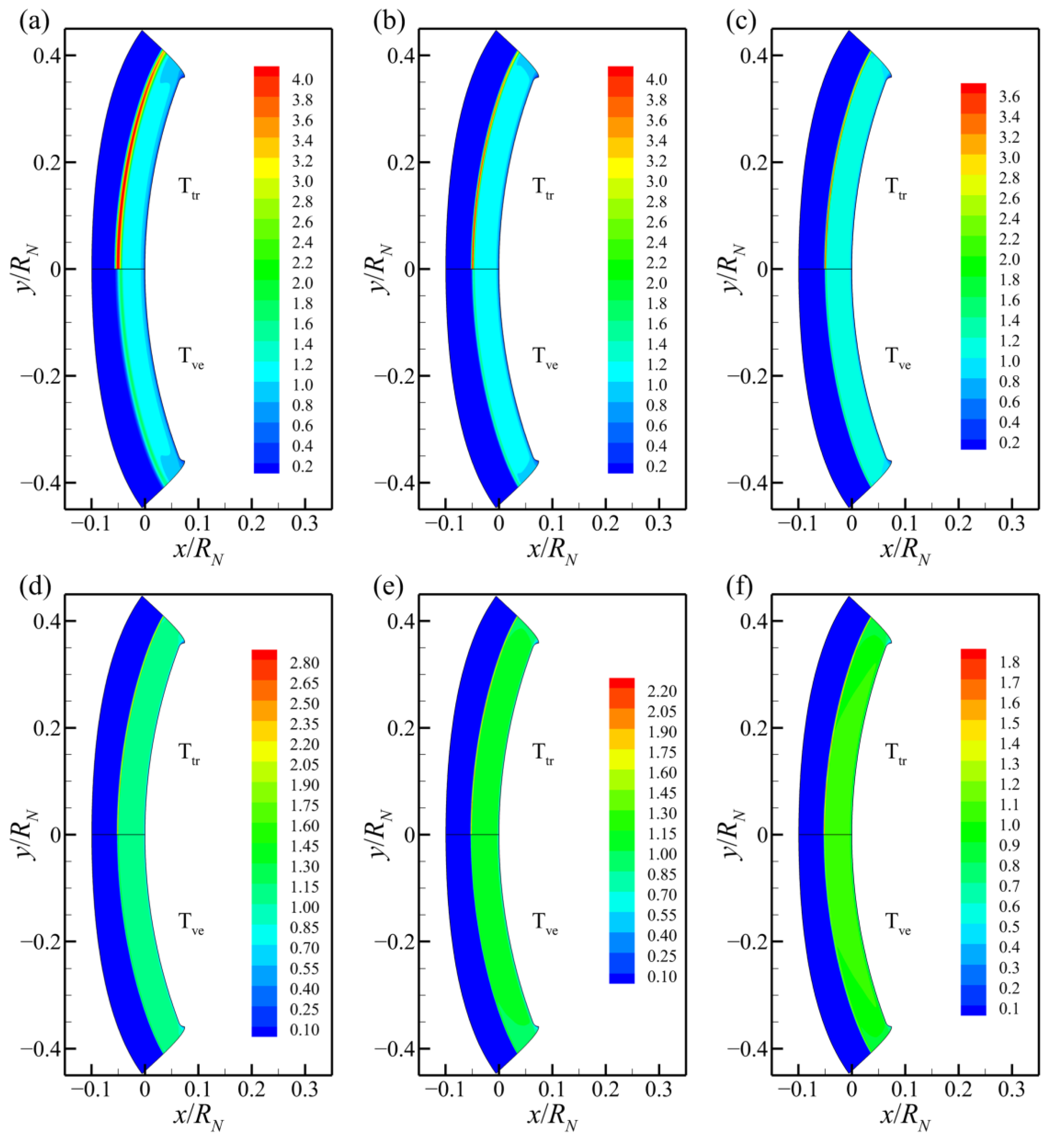
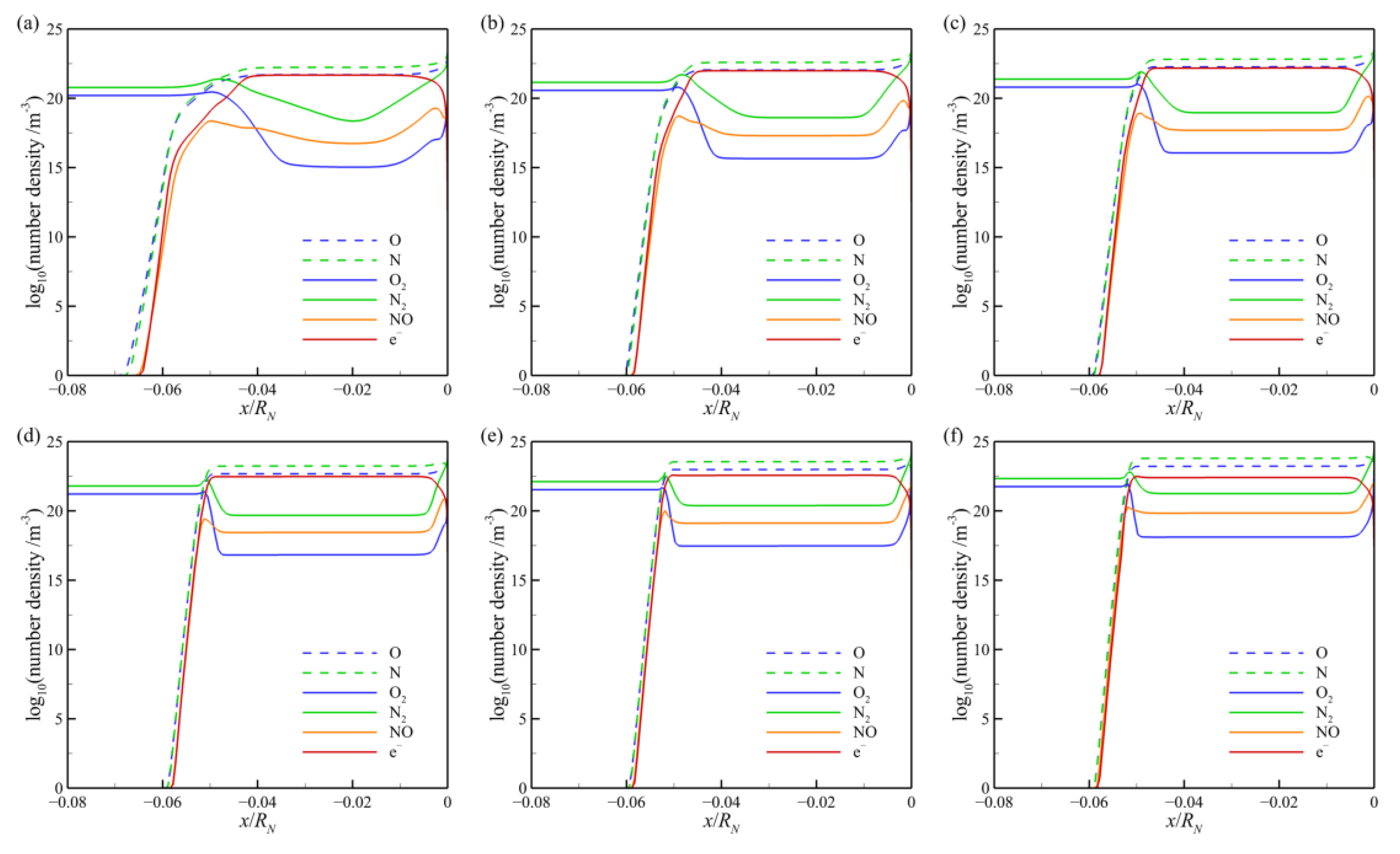
3.2. Thermochemical Nonequilibrium Flowfield

Figure 5 compares the translational-rotational temperature T_tr and vibrational-electronic temperature T_ve in the Fire II flowfield throughout the trajectory from t = 1634 s to 1645 s. At t = 1634 s, there is a remarkable difference between T_tr and T_ve in a distance closely behind the bow shock, which suggests the translational-rotational and vibrational-electronic energy modes are highly in nonequilibrium in this region. As time goes on with the altitude and velocity down, the thermodynamic nonequilibrium tends to be weakened steadily and the total level of magnitude of temperature also decreases gradually. From t = 1637 s to 1645 s, T_tr and T_ve have become consistent in most areas of the shock layer. For all cases, both T_tr and T_ve exceed 10⁴ K in the shock layer around the Fire II forebody, and the peak of the translational-rotational temperature even reaches up to 44,000 K at t = 1634 s. Such extreme high temperature directly leads to the harsh aerothermal environment for Earth reentry and results in significant radiative heating [19]. Figure 6 presents the number densities of the species O, N, O₂, N₂, NO, and e⁻ along the stagnation line for each case. The high atomic and electron concentrations demonstrate the strong dissociation and ionization reactions of air in the reentry shock layer of Fire II. At t = 1634 s, the number density of each species changes remarkably along the stagnation line, while at the following trajectory points, such variations become more and more unnoticeable and the concentration of each species approaches a constant in most regions of the shock layer. Due to the high ionization, the number density of electrons (that is the sum of the number densities of all positive ions, such as O⁺, N⁺, and NO⁺) is greater than 10²¹ m⁻³ in most areas of the shock layer. The free electrons and ions constitute a plasma sheath around the reentry vehicle, which absorbs the radio-frequency radiation and causes the communication blackout [60].

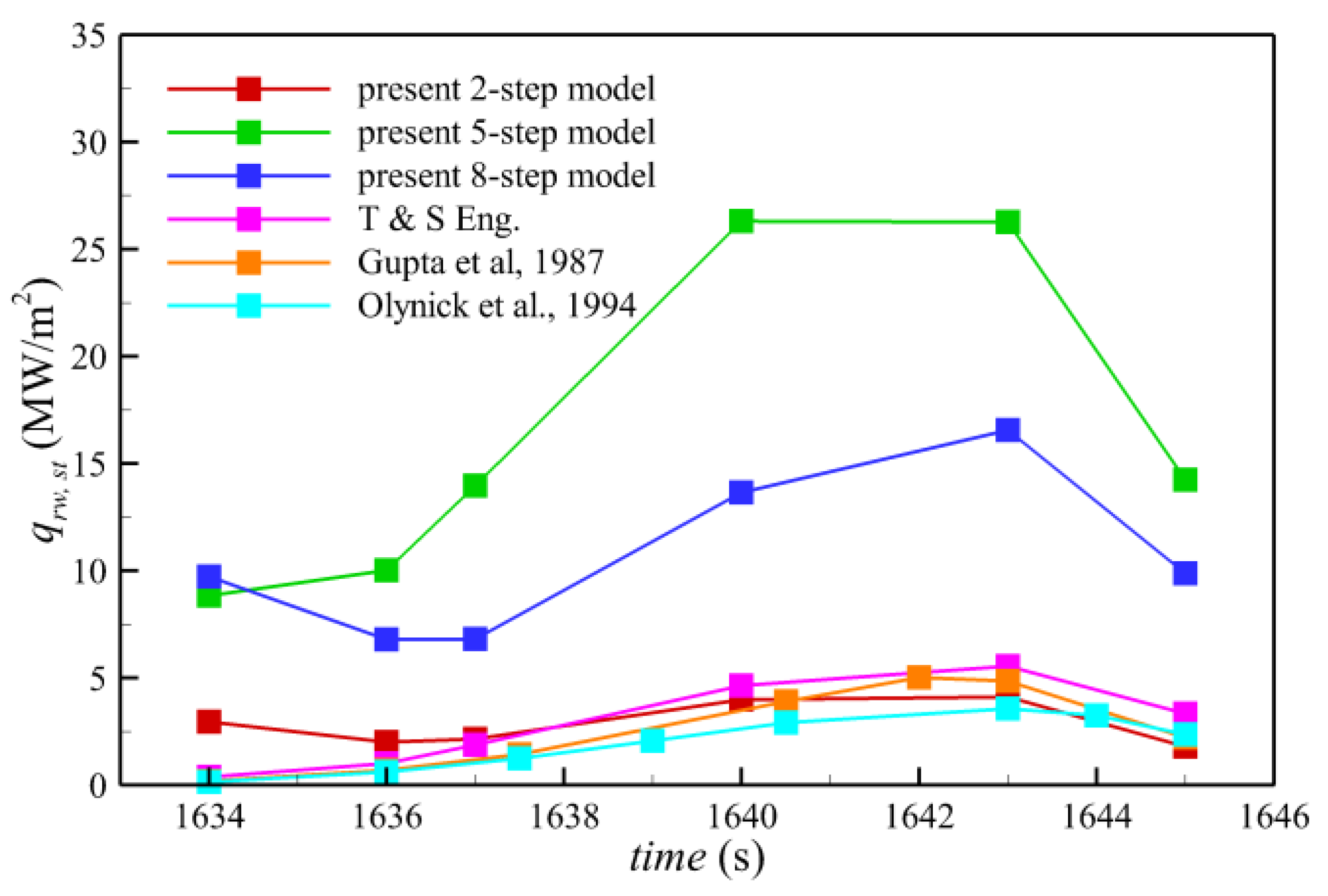
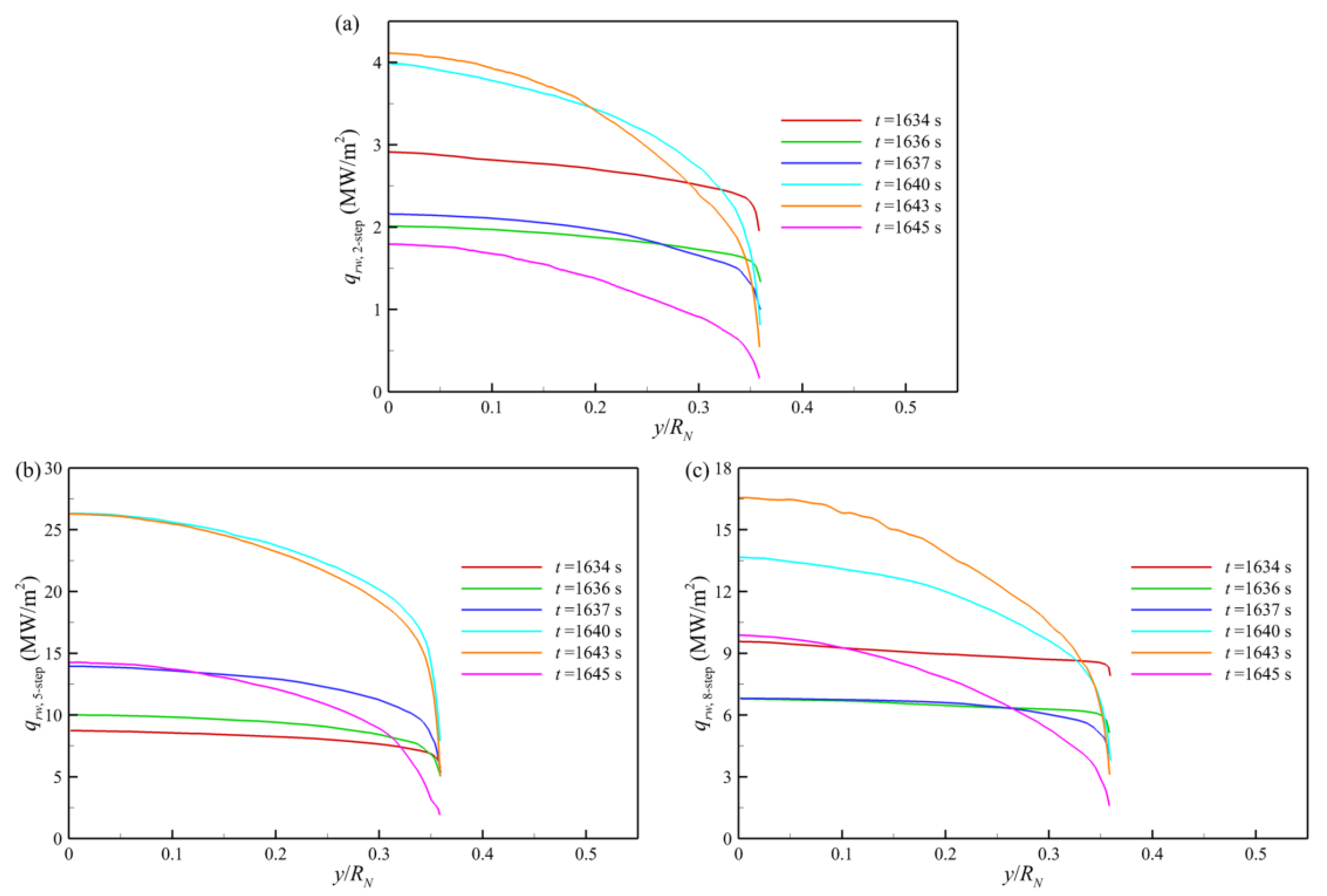
3.3. Radiative Heating

The radiative transfer is solved by employing the radiation–flow uncoupling algorithm, in which the radiation is calculated only once based on the convergent flowfield solution using the methods in Section 2. Compared with the radiation–flow coupling approach, although the uncoupling simulation compromises some accuracy in physics, the procedure really can greatly reduce the computing power and time. Figure 7 compares the results of radiative heating at the stagnation point calculated by Tauber and Sutton’s (T & S) engineering relationship [61], Gupta et al. [37], Olynick et al. [38], and the present TS method with the two-step, five-step, and eight-step models, respectively. The T & S relation is expressed as follows:

$$q_{rw,stag}=4.736\times {10}^8{R}_N^a{\rho }_{\infty }^{b}f\left(V_{\infty }\right)({\mathrm{W}/\mathrm{m}}^2)$$

(13)

where R_N is the vehicle nose radius; ρ_∞ and V_∞ are the freestream density and velocity; a and b are empirical exponents; f is a tabulated function of freestream velocity V_∞. The detailed descriptions of a, b, and f can be found in Ref. [61].

Gupta et al. developed a RAD code accounting for the molecular band, continuum, and atomic line transitions. They employed a detailed frequency dependence of the absorption coefficients to integrate over the radiation spectrum and used the TS approximation for integrating over physical space, but only limited to the stagnation region. Olynick et al. developed a GIANTS/NOVAR code to obtain values of the stagnation radiation intensity in the 0.2 and 6.2 eV range. They used a “smeared band” approximation instead of a line-by-line approach to account for the air radiation properties of the molecular band systems and reduce the total number of spectral points. Even doing so, Olynick et al. still needed to perform TS integration at each radiation grid point consisting of around 1000 frequency points for calculating absorption and emission coefficients, which is very time-consuming. Gupta et al. and Olynick et al. both implemented the radiation–flow coupling simulation with nonequilibrium chemistry. Figure 7 shows that the radiative heat fluxes calculated by the TS approximation with the step models are mostly greater than those obtained by the T & S relation, Gupta et al., and Olynick et al. In fact, compared with the coupling simulation, the present radiation–flow uncoupling method should predict the higher level of radiative heating [22], which is reasonable and can be seen as the conservative upper limit in the engineering application.

Although the noticeable differences can be seen among the radiative heat fluxes of different methods, the orders of magnitude of all the data are basically the same and they show a similar tendency, first an increase and then decrease. The five-step model gives the greatest stagnation radiative heat transfer, while the results of the two-step model are the smallest. Unexpectedly, although the two-step model is coarsest in spectral space, it predicts the closest values with those of the T & S relation, Gupta et al. [37], and Olynick et al. [38] compared to the other two models. However, we cannot simply deduce that the two-step model is the best option because it is just only applicable for Fire II trajectory points. The final evaluation needs more experimental data and further high-resolution numerical simulation in the future.

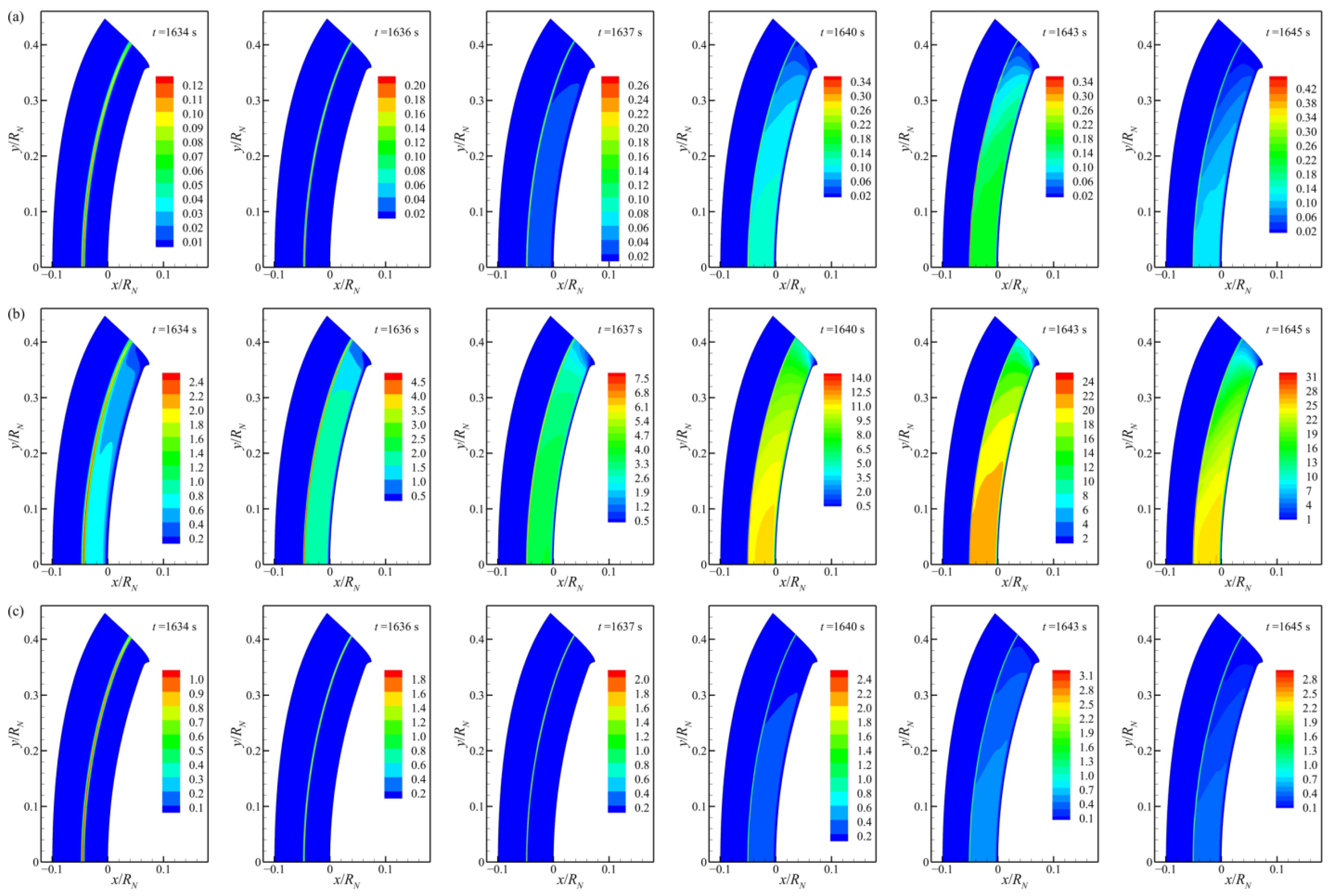
3.4. Radiation Field

Except for the more affordable time cost than that of the coupling simulation, the present radiation–flow uncoupling algorithm can provide the more detailed information than those of the engineering methods, not only the radiative heat transfer at the stagnation point but also the radiative heating distribution on the vehicle surface and the radiation characteristics in the whole flowfield. The latter radiation distributions in the flowfield are rarely shown in the previous literature [37,38,39,40,41] but may play some important roles in understanding the mechanism of radiative heating and designing the thermal protection system of atmospheric entry vehicles in the future [6]. Figure 8 shows the radiative heating over the whole surface of the Fire II forebody predicted by the TS approximation with the two-step, five-step, and eight-step models, respectively. If the heat transfer of magnitude is not taken into consideration, the tendencies obtained by the three models are basically consistent. The radiative heating varies flatly over the whole vehicle surface for the cases from t = 1634 s to 1637 s, while it becomes more bending for the following cases from t = 1640 s to 1645 s. Figure 9 shows the distributions of the Planck-mean absorption coefficient around the Fire II forebody throughout the trajectory calculated by the two-step, five-step, and eight-step models, respectively. The Planck-mean absorption coefficient is one of the most important average forms that describes the total emission from a fluid element and indicates the level of radiative heat loss from the nearly optically thin flowfield. The Planck-mean absorption coefficient for the present step model is defined as follows:

$${\kappa }_{\mathrm{P}}=\frac{{\displaystyle \sum _m{\kappa }_m{\displaystyle {\int }_m{I}_{b\nu }\mathrm{d}\nu }}}{{\displaystyle {\int }_0^{\infty }{I}_{b\nu }\mathrm{d}\nu }}=\frac{\pi {\displaystyle \sum _m{\kappa }_m{\displaystyle {\int }_m{I}_{b\nu }\mathrm{d}\nu }}}{\sigma T^4}$$

(14)

where m is the spectral step index, κ_m is the absorption coefficient for the m-th step, I_bν is the spectral blackbody intensity at radiation frequency ν, σ is the Stefan–Boltzmann constant, and T is the temperature. In the present hypersonic nonequilibrium flow, κ_P is calculated using the vibrational-electronic temperature [62].

Figure 9 shows that κ_P is remarkable only in the shock layer, particularly nearly behind the bow shock with peak values, while κ_P is very small in the freestream. It suggests that the radiation energy transfer mainly occurs in the high-temperature shock layer. The five-step model predicts the greatest κ_P, the eight-step model second, and the two-step model the smallest. As time goes on with the altitude and velocity down, the total level of κ_P grows gradually. Although the temperature in the shock layer decreases as shown in Figure 5 and makes a negative contribution to radiative transfer as the Fire II flight altitude descends, the air density increase significantly promotes the radiation effect in the flowfield. The results of the three-step models all support this point. Another interesting thing is that κ_P predicted by the two-step model shows the Fire II shock layer is close to being optically thin with the optical thickness being an order of magnitude of 10⁻², while the results of the five-step and eight-step models do not agree with this, which can only be clarified further in the future using the more detailed radiation property model, such as the line-by-line or narrowband calculations [57]. Generally, the present radiation–flow uncoupling procedure is a good selection with higher efficiency in time cost than the coupling method to provide rich radiation information on the whole hypersonic nonequilibrium flowfield of Fire II reentry that the engineering methods cannot make.

4. Conclusions

A radiation–flowfield uncoupling procedure is developed to simulate the Fire II trajectory points aimed at studying the radiative heating in the thermochemical nonequilibrium flowfield for Earth reentry at hypervelocity above 10 km/s. The radiative transfer is integrated only once by the TS approximation with the nongray step model based on the flow solution obtained using an in-house N–S solver PHAROS. It is naturally more efficient in computational cost than the coupled scheme, and also provides reasonable and more detailed information on the aerothermal environment than the engineering relations which always can only calculate the aerodynamic heat flux at the stagnation point of reentry vehicles.

The results of Fire II cases throughout the trajectory from t = 1634 s to 1645 s show that the radiative heating grows first and then decreases with the order of magnitude of 1 MW/m², which is comparable to the convective heating and even exceeds the latter. Although there are remarkable differences among the two-, five-, and eight-step models, the three models all show essentially consistent trends in predictions of radiative transfer. The uncoupling calculated radiative heating can be regarded as the upper limit in the engineering application. In the future, more efforts need to be made to clarify the level of the optical thickness for the flowfield of Earth reentry vehicles at hypervelocity above 10 km/s, which the two-step model predicts to be optically thin, while the five- and eight-step models do not agree. The present scheme can also provide more radiation information in the nonequilibrium flowfield than the previous engineering relations.

Due to the fact that the flowfield establishes far more quickly than the vehicle flies down for Earth reentry, it can perform steady flow simulation at each trajectory point. Therefore, the present radiation–flow uncoupling algorithm using a nongray step model with moderate efficiency and reasonable accuracy is promising to solve the real-time problem in engineering for predicting both convective and radiative heating to the atmospheric reentry vehicle in the future.

References

1. Sziroczak, D.; Smith, H.A. Review of Design Issues Specific to Hypersonic Flight Vehicles. Prog. Aeronaut. Sci. 2016, 84, 1–28. [Google Scholar] [CrossRef] [Green Version]
2. Johnston, C.O.; Mazaheri, A. Impact of Non-Tangent-Slab Radiative Transport on Flowfield–Radiation Coupling. J. Spacecr. Rocket. 2018, 55, 899–913. [Google Scholar] [CrossRef]
3. Hao, J.; Wang, J.; Lee, C. Numerical study of hypersonic flows over reentry configurations with different chemical nonequilibrium models. Acta Astronaut. 2016, 126, 1–10. [Google Scholar] [CrossRef]
4. Maier, W.T.; Needels, J.T.; Garbacz, C. SU2-NEMO: An open-source framework for high-mach nonequilibrium multi-species flows. Aerospace 2021, 8, 193. [Google Scholar] [CrossRef]
5. Hao, J.; Wang, J.; Lee, C. Assessment of vibration-dissociation coupling models for hypersonic nonequilibrium simulations. Aerosp. Sci. Technol. 2017, 67, 433–442. [Google Scholar] [CrossRef]
6. Wang, J.; Han, F.; Lei, L. Numerical study of high-temperature nonequilibrium flow around reentry vehicle coupled with thermal radiation. Fluid Dyn. Mater. Process. 2020, 16, 601–613. [Google Scholar] [CrossRef]
7. Brandis, A.M.; Saunders, D.A.; Johnston, C.O. Radiative heating on the after-body of Martian entry vehicles. J. Thermophys. Heat Transf. 2020, 34, 66–77. [Google Scholar] [CrossRef]
8. Santos Fernandes, L.; Lopez, B.; Lino da Silva, M. Computational fluid radiative dynamics of the Galileo Jupiter entry. Phys. Fluids 2019, 31, 106104. [Google Scholar] [CrossRef]
9. Bansal, A.; Modest, M.F.; Levin, D.A. Multi-scale k-distribution model for gas mixtures in hypersonic nonequilibrium flows. J. Quant. Spectrosc. Radiat. Transf. 2011, 112, 1213–1221. [Google Scholar] [CrossRef]
10. Jo, S.M.; Kwon, O.J.; Kim, J.G. Stagnation-point heating of Fire II with a non-Boltzmann radiation model. Int. J. Heat Mass Transf. 2020, 153, 119566. [Google Scholar] [CrossRef]
11. Feldick, A.M.; Modest, M.F.; Levin, D.A. Closely coupled flowfield-radiation interactions during hypersonic reentry. J. Thermophys. Heat Transf. 2011, 25, 481–492. [Google Scholar] [CrossRef] [Green Version]
12. Sohn, I.; Li, Z.; Levin, D.A. Effect of Nonlocal Vacuum Ultraviolet Radiation on a Hypersonic Nonequilibrium Flow. J. Thermophys. Heat Transf. 2012, 26, 393–406. [Google Scholar] [CrossRef]
13. Surzhikov, S.T. Radiative gasdynamics of the nose surface of the Apollo-4 command module at its superobrital reentry. Fluid Dyn. 2017, 52, 815–831. [Google Scholar] [CrossRef]
14. Lamet, J.M.; Babou, Y.; Riviere, P. Radiative transfer in gases under thermal and chemical nonequilibrium conditions: Application to earth atmospheric re-entry. J. Quant. Spectrosc. Radiat. Transf. 2008, 109, 235–244. [Google Scholar] [CrossRef]
15. Sohn, I.; Bansal, A.; Levin, D.A.; Modest, M.F. Advanced radiation calculations of hypersonic reentry flows using efficient databasing schemes. J. Thermophys. Heat Transf. 2010, 24, 623–637. [Google Scholar] [CrossRef]
16. Rahmanpour, M.; Ebrahimi, R.; Shams, M. Numerically gas radiation heat transfer modeling in chemically nonequilibrium reactive flow. Heat Mass Transf. 2011, 47, 1659–1670. [Google Scholar] [CrossRef]
17. Wang, J.; Ju, P.; Lei, L. A two-dimensional finite volume scheme solving the axisymmetric radiative heat transfer based on general structured grids. J. Therm. Sci. Technol. 2019, 14, JTST0004. [Google Scholar] [CrossRef] [Green Version]
18. Andrienko, D.A.; Surzhikov, S.; Shang, J. View-Factor Approach as a Radiation Model for the Reentry Flowfield. J. Spacecr. Rocket. 2016, 53, 74–83. [Google Scholar] [CrossRef]
19. Anderson, J.D. An engineering survey of radiating shock layers. AIAA J. 1969, 7, 1665–1675. [Google Scholar] [CrossRef]
20. Olstad, W.B. Nongray radiating flow about smooth symmetric bodies. AIAA J. 1971, 9, 122–130. [Google Scholar] [CrossRef]
21. Greendyke, R.B.; Hartung, L.C. Approximate method for the calculation of nonequilibrium radiative heat transfer. J. Spacecr. Rocket. 1991, 28, 165–171. [Google Scholar] [CrossRef]
22. Anderson, J.D. Hypersonic and High Temperature Gas Dynamics, 2nd ed.; AIAA, Inc.: Reston, VA, USA, 2006; pp. 769–773. [Google Scholar]
23. Andrienko, D.A.; Surzhikov, S.T.; Shang, J.S. Spherical harmonics method applied to the multi-dimensional radiation transfer. Comput. Phys. Commun. 2013, 184, 2287–2298. [Google Scholar] [CrossRef]
24. Mazaheri, A.; Johnston, C.O.; Sefidbakht, S. Three-dimensional radiation ray-tracing for shock-layer radiative heating simulations. J. Spacecr. Rocket. 2013, 50, 485–493. [Google Scholar] [CrossRef]
25. Chai, J.C.; Lee, H.O.S.; Patankar, S.V. Finite volume method for radiation heat transfer. J. Thermophys. Heat Transf. 1994, 8, 419–425. [Google Scholar] [CrossRef]
26. Wang, J.; Hao, J.; Du, G. Thermal radiation solving method library for the reentry vehicle flowfield simulation. K. Cheng Je Wu Li Hsueh Pao/J. Eng. Thermophys. 2017, 38, 1972–1979. [Google Scholar]
27. Ozawa, T.; Levin, D.A.; Wang, A. Development of Coupled Particle Hypersonic Flowfield-Photon Monte Carlo Radiation Methods. J. Thermophys. Heat Transf. 2010, 24, 612–622. [Google Scholar] [CrossRef] [Green Version]
28. Andrienko, D.A.; Surzhikov, S.T. P1 approximation applied to the radiative heating of descent spacecraft. J. Spacecr. Rocket. 2012, 49, 1088–1098. [Google Scholar] [CrossRef]
29. Stanley, S.A.; Carlson, L.A. Effects of shock wave precursors ahead of hypersonic entry vehicles. J. Spacecr. Rocket. 1992, 29, 190–197. [Google Scholar] [CrossRef]
30. Hartung, L.C.; Mitcheltree, R.A.; Gnoffo, P.A. Coupled radiation effects in thermochemical nonequilibrium shock-capturing flowfield calculations. J. Thermophys. Heat Transf. 1994, 8, 244–250. [Google Scholar] [CrossRef] [Green Version]
31. Wright, M.J.; Bose, D.; Olejniczak, J. Impact of flowfield-radiation coupling on aeroheating for titan aerocapture. J. Thermophys. Heat Transf. 2005, 19, 17–27. [Google Scholar] [CrossRef]
32. Johnston, C.O.; Hollis, B.R.; Sutton, K. Nonequilibrium stagnation-line radiative heating for Fire II. J. Spacecr. Rocket. 2008, 45, 1185–1195. [Google Scholar] [CrossRef] [Green Version]
33. Bauman, P.T.; Stogner, R.; Carey, G.F. Loose-coupling algorithm for simulating hypersonic flows with radiation and ablation. J. Spacecr. Rocket. 2011, 48, 72–80. [Google Scholar] [CrossRef]
34. Johnston, C.O.; Brandis, A.M. Features of afterbody radiative heating for earth entry. J. Spacecr. Rocket. 2015, 52, 105–119. [Google Scholar] [CrossRef]
35. Viviani, A.; Pezzella, G. Aerodynamic and Aerothermodynamic Analysis of Space Mission Vehicles; Springer International Publishing: Heidelberg, Germany, 2015; pp. 199–204. [Google Scholar]
36. Tauber, M.E.; Palmer, G.E.; Yang, L. Earth atmospheric entry studies for manned Mars missions. J. Thermophys. Heat Transf. 1992, 6, 193–199. [Google Scholar] [CrossRef]
37. Gupta, R. Navier-Stokes and viscous shock-layer solutions for radiating hypersonic flows. In Proceedings of the AIAA 22nd Thermophysics Conference, Honolulu, HI, USA, 8–10 June 1987. [Google Scholar]
38. Olynick, D.; Henline, W.; Chamberg, L. Comparisons of coupled radiative Navier-Stokes flow solutions with the project Fire II flight data. In Proceedings of the 6th AIAA/AMSE Joint Thermophysics and Heat Transfer Conference, Colorado Springs, CO, USA, 20–23 June 1994. [Google Scholar]
39. Palmer, G.E.; White, T.; Pace, A. Direct coupling of the NEQAIR radiation and DPLR CFD codes. J. Spacecr. Rocket. 2011, 48, 836–845. [Google Scholar] [CrossRef]
40. Soucasse, L.; Scoggins, J.B.; Rivière, P. Flow-radiation coupling for atmospheric entries using a Hybrid Statistical Narrow Band model. J. Quant. Spectrosc. Radiat. Transf. 2016, 180, 55–69. [Google Scholar] [CrossRef]
41. Bonin, J.; Mundt, C. Full three-dimensional Monte Carlo radiative transport for hypersonic entry vehicles. J. Spacecr. Rocket. 2019, 56, 44–52. [Google Scholar] [CrossRef]
42. Park, C. Assessment of two-temperature kinetic model for ionizing air. J. Thermophys. Heat Transf. 1989, 3, 233–244. [Google Scholar] [CrossRef]
43. Liu, Y.; Vinokur, F.S. A comparison of Internal Energy Calculation Methods for Diatomic Molecules. Phys. Fluids A 1990, 2, 1888–1902. [Google Scholar] [CrossRef]
44. Gupta, R.N.; Yos, J.M.; Thompson, R.A. A Review of Reaction and Thermodynamic and Transport Properties for an 11-Species Air Model for Chemical and Thermal Nonequilibrium Calculations to 30,000 K; NASA RP 1232; National Aeronautics and Space Administration: Washington, DC, USA, 1990. [Google Scholar]
45. Wang, J. Numerical Study on Coupled Chemical Nonequilibrium and Thermal Radiation Effects in High Speed and High Temperature Flows. Ph.D. Thesis, Beihang University, Beijing, China, 2015. [Google Scholar]
46. Gnoffo, P.A.; Gupta, R.N.; Shinn, J.L. Conservation Equations and Physical Models for Hypersonic Air Flows in Thermal and Chemical Nonequilibrium; NASA TP 2867; National Aeronautics and Space Administration: Washington, DC, USA, 1989. [Google Scholar]
47. Shoev, G.; Oblapenko, G.; Kunova, O. Validation of vibration-dissociation coupling models in hypersonic non-equilibrium separated flows. Acta Astronaut. 2018, 144, 147–159. [Google Scholar] [CrossRef]
48. Millikan, R.C.; White, D.R. Systematics of Vibrational Relaxation. J. Chem. Phys. 1963, 39, 3209–3213. [Google Scholar] [CrossRef]
49. Boyd, D. Rotational and vibrational nonequilibrium effects in rarefied hypersonic flow. J. Thermophys. Heat Transf. 1990, 4, 478–484. [Google Scholar] [CrossRef] [Green Version]
50. Hao, J.; Wang, J.; Lee, C. Development of a Navier-Stokes code for hypersonic nonequilibrium simulations. In Proceedings of the 21st AIAA International Space Planes and Hypersonics Technologies Conference, Xiamen, China, 6–9 March 2017. [Google Scholar]
51. MacCormack, R.W.; Candler, G.V. The solution of the Navier-Stokes equations using Gauss-Seidel line relaxation. Comput. Fluids 1989, 17, 135–150. [Google Scholar] [CrossRef]
52. Van Leer, B. Towards the ultimate conservative difference scheme. J. Comput. Phys. 1997, 135, 229–248. [Google Scholar] [CrossRef]
53. Wright, M.J.; Candler, G.V.; Bose, D. Data-parallel line relaxation method for the Navier-Stokes equations. AIAA J. 1998, 36, 1603–1609. [Google Scholar] [CrossRef]
54. Hao, J.; Wang, J.; Gao, Z. Comparison of transport properties models for numerical simulations of Mars entry vehicles. Acta Astronaut. 2017, 130, 24–33. [Google Scholar] [CrossRef]
55. Carlson, L.A. Approximations for hypervelocity nonequilibrium radiating, reacting, and conducting stagnation regions. J. Thermophys. Heat Transf. 1989, 3, 380–388. [Google Scholar] [CrossRef]
56. Carlson, L.A.; Bobskill, G.J.; Greendyke, R.B. Comparison of vibration-dissociation coupling and radiative transfermodels for AOTV/AFE flowfields. J. Thermophys. Heat Transf. 1990, 4, 16–26. [Google Scholar] [CrossRef]
57. Modest, M.F. Radiative Heat Transfer, 2nd ed.; Academic Press: San Diego, CA, USA, 2003; pp. 269–271; 288–346. [Google Scholar]
58. Bertin, J.J.; Cummings, R.M. Critical hypersonic aerothermodynamic phenomena. Annu. Rev. Fluid Mech. 2006, 38, 129–157. [Google Scholar] [CrossRef] [Green Version]
59. Scalabrin, L.C. Numerical Simulation of Weakly Ionized Hypersonic Flow over Reentry Capsules. Ph.D. Thesis, University of Michigan, Ann Arbor, MI, USA, 2007. [Google Scholar]
60. Ramjatan, S.; Lani, A.; Boccelli, S. Blackout analysis of Mars entry missions. J. Fluid Mech. 2020, 904, A26. [Google Scholar] [CrossRef]
61. Tauber, M.E.; Sutton, K. Stagnation-point radiative heating relations for Earth and Mars entries. J. Spacecr. Rocket. 1991, 28, 40–42. [Google Scholar] [CrossRef]
62. Mazzoni, C.M.; Lentini, D.; D’Ammando, G. Evaluation of radiative heat transfer for interplanetary re-entry under vibrational nonequilibrium conditions. Aerosp. Sci. Technol. 2013, 28, 191–197. [Google Scholar] [CrossRef]
63. Anderson, J.D. Heat transfer from a viscous nongray radiating shock layer. AIAA J. 1968, 6, 1570–1573. [Google Scholar] [CrossRef]
64. Knott, P.R.; Carlson, L.A.; Nerem, R.M. A further note on shock-tube measurements of end-wall radiative heat transfer in air. AIAA J. 1969, 7, 2170–2172. [Google Scholar] [CrossRef]
Figure 1. Geometry and mesh of Fire II.
Aerospace 09 00219 g001
Figure 2. Convective heating at the stagnation point of Fire II predicted by the present algorithm (present), Anderson’s engineering relation (Anderson Eng.), Olynick et al., and Gupta et al.
Aerospace 09 00219 g002
Figure 3. Forebody convective heating along the Fire II surface throughout the trajectory from t = 1634 s to t = 1645 s.
Aerospace 09 00219 g003
Figure 4. Forebody convective heating at t = 1636 s predicted by the present algorithm (present), DPLR, and LAURA codes.
Aerospace 09 00219 g004
Figure 5. Temperature distribution in the Fire II flowfield (unit: 104 K): (a) t = 1634 s; (b) t = 1636 s; (c) t = 1637 s; (d) t = 1640 s; (e) t = 1643 s; (f) t = 1645 s.
Aerospace 09 00219 g005
Figure 6. Number density of species along the stagnation line: (a) t = 1634 s; (b) t = 1636 s; (c) t = 1637 s; (d) t = 1640 s; (e) t = 1643 s; (f) t = 1645 s.
Aerospace 09 00219 g006
Figure 7. Radiative heating at the stagnation point of Fire II throughout the trajectory predicted by the present algorithm with 2-step model, 5-step model, 8-step model, T & S engineering relation, Gupta et al., and Olynick et al.
Aerospace 09 00219 g007
Figure 8. Forebody radiative heating throughout the trajectory predicted by (a) two-step model; (b) five-step model; (c) eight-step model.
Aerospace 09 00219 g008
Figure 9. Planck-mean absorption coefficient throughout the trajectory (unit: m−1): (a) two-step model; (b) five-step model; (c) eight-step model.
Aerospace 09 00219 g009