Configuration Optimization for Free-Floating Space Robot Capturing Tumbling Target

Abstract

The maximum contact force is one of the most important indicators for contact problems. In this paper, the configuration optimization is conducted to reduce the maximum contact force for a free-floating space robot capturing tumbling target. First, the dynamics model of a free-floating space robot is given, with which the inertial properties perceived at the end-effector can be derived. Combing the inertial properties of the contact bodies, a novel concept of integrated effective mass is proposed. It tries to transform the complex contact process into the energy change of a virtual single body with integrated effective mass. On this basis, a more general continuous contact model is established, which is also suitable for non-central collisions between space robot and the tumbling target. Thereafter, the maximum contact force is derived as an important indicator for the null-space optimization method to reduce the maximum contact force. Finally, numerical simulations with a 3-degree-of-freedom free-floating space robot and a 7-degree-of-freedom free-floating space robot, as the research objects, are carried out respectively and the results show the effectiveness of the method proposed.

1. Introduction

Due to the characteristics of microgravity, high vacuum, and strong radiation in space, astronauts carrying out space missions will face extremely high risks. Space robots, with their outstanding advantages in terms of strong adaptability to the space environment and freedom from physiological conditions, have gradually become the main force in space exploration [1,2,3]. In recent years, with the continuous development of space exploration, capturing non-cooperative targets has attracted much attention, as the technique is expected to be applied for functions such as the removal of debris from orbit and servicing broken satellites for repair [4,5,6].

Scholars have conducted research on related technologies in the capture of non-cooperative targets. It is generally known that an entire capture task contains three phases: the target-chasing control phase, which is also called the pre-contact phase; the contact phase between the target and end-effector of the space robot; and the stabilization control phase of tumbling motion, which is also called the post-contact phase [7,8]. Most research focuses on the pre-contact phase to optimize the capture configuration or follow an optimal trajectory [9,10,11,12], and the post-contact phase to detumble the non-cooperative target or reduce the base attitude disturbance [13,14,15,16]. In this paper, based on the analysis of the contact phase, which emphasizes contact modelling, the capture configuration is optimized to minimize the maximum contact force.

For the contact-modelling problem, there are generally two different approaches from the perspective of whether the contact process is assumed to be continuous or not. The first approach is usually called discrete contact dynamics modelling method, which assumes that the contact is an instantaneous phenomenon, and that the configuration of contacting bodies does not change significantly. Therefore, the contact effect in this approach is usually regarded as a contact–impact impulse. Most of the early studies on the contact problem between space robots and targets are based on the first approach, and the minimization of the contact-impact impulse becomes one concern to reduce the effect caused by contact [17,18,19,20,21,22]. It is simple and efficient to make a contact dynamics analysis of a space robot by the first approach, but only the contact–impact impulse can be calculated and no more detailed information during the contact process can be obtained. The second approach is usually called the continuous contact dynamics modelling method, which is based on the fact that the interaction forces act in a continuous manner during the contact. Some contact force models are proposed based on the second approach, for example, the Hunt–Crossley, Herbert–McWhannell, Lankarain–Nikravesh, Zhiying–Qishao and Lee–Wang models [23,24,25]. Several of these models have been used to analyze the contact process between a space robot and a target [26,27,28,29]. The analytical expression of contact force can be obtained by this approach and thus the detailed information during the contact process can also be described. However, it may not be very efficient to directly apply these models to a space robot system, because it requires all of the motion equations integrated over the entire contact period. Refer to the concept of virtual mass proposed in [30]; an effective mass concept is proposed for the contact modelling of space robots performing contact tasks [31,32], and this method is further extended to solve the contact problem of flexible space robots [33]. Computational efficiency can be improved by this method, and an analytical solution of the contact information is given, but it is based on the assumption that only a central collision occurs.

As the contact–impact impulse is the integration of contact force over the entire contact period, the minimization of the contact–impact impulse is not equivalent to the minimization of the maximum contact force. If the maximum contact force exceeds the physical limit the space robot allows, the robot itself or the target may be severely damaged. Therefore, the maximum contact force should command attention and, actually, it is one of the most important indicators for contact problems [34]. This paper is focused on continuous contact modelling and configuration optimization to reduce the maximum contact force for free-floating space robot capturing tumbling target. The main contributions of this paper are: (1) A novel concept of integrated effective mass that integrates the inertial properties of the contact bodies is proposed in an attempt to transform the complex contact process into the energy change of a virtual single body with integrated effective mass; (2) A more general continuous contact model is established, which is also suitable for non-central collisions between a space robot and a tumbling target; (3) The maximum contact force is derived as an important indicator for the null-space optimization method to reduce the maximum contact force. It is worth noting that the concept of integrated effective mass and the continuous contact model proposed in this paper are common to both redundant robots and non-redundant robots. However, due to the use of the null-space optimization algorithm, the optimization part is only applicable to redundant robots. If there is a need to optimize the maximum contact force for a non-redundant robot, the task constraints can be reduced or other optimization methods, such as the Particle Swarm Optimization (PSO), can be used.

The rest of this paper is organized as follows. The analytical expression of integrated effective mass is derived in Section 2. On this basis, the continuous contact model between a free-floating space robot and a tumbling target is given in Section 3, in which the maximum contact force expression is also derived. Thereafter, in Section 4, the configuration optimization based on the null-space method is conducted for capturing a tumbling target, and the effectiveness of the proposed method is verified by numerical simulations in Section 5. Finally, conclusions are drawn in Section 6.

2. Integrated Effective Mass

A novel integrated effective mass concept is first proposed in this section. It integrates the inertial properties of the contact bodies and tries to transform the complex contact process into the energy change of a virtual single body with integrated effective mass.

2.1. Inertial Properties Perceived at End-Effector

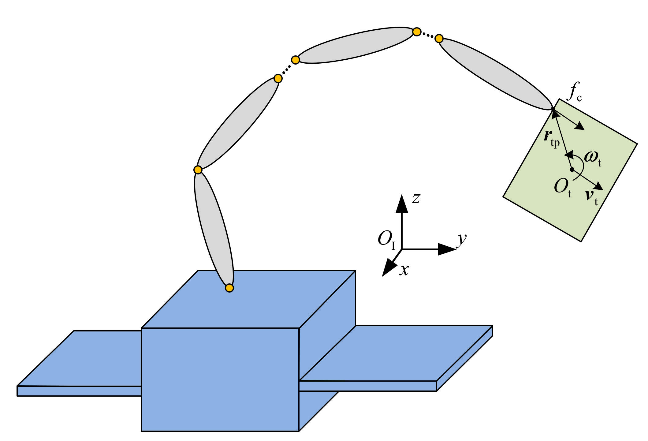
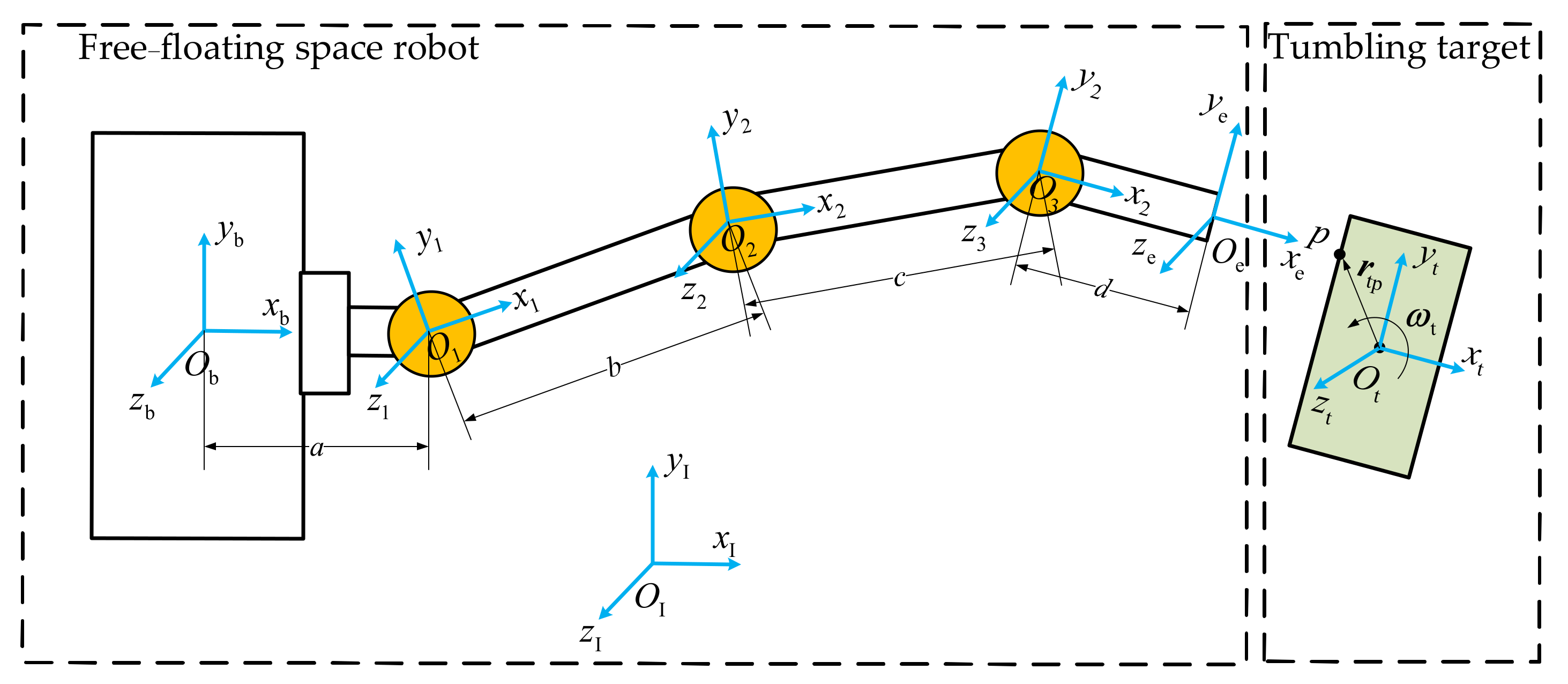
Generally, the contact occurs at the end-effector of a free-floating space robot as shown in Figure 1. Therefore, the inertial properties perceived at the end-effector must be analyzed first. All variables in the following are expressed in the inertial frame $O_{\mathrm{I}}$ if not stated.

The dynamics model of a free-floating space robot with n revolute joints is expressed in the following general form [7,8]:

$$\mathit{H}\ddot{\mathit{\varphi }}+\mathit{C}={\mathit{F}}_{b\_m}+{\mathit{J}}_{\mathrm{b}\_\mathrm{m}}^{\mathrm{T}}{\mathit{F}}_e,$$

(1)

where $\mathit{H}$ is the inertial matrix, $\mathit{C}$ is the velocity-dependent nonlinear term; $\ddot{\mathit{\varphi }}={\left[{\ddot{\mathit{x}}}_{\mathrm{b}},\ddot{\mathit{\theta }}\right]}^{\mathrm{T}}$ with ${\ddot{\mathit{x}}}_b=\left[{\dot{\mathit{v}}}_0,{\dot{\mathit{\omega }}}_0\right]$ and $\ddot{\mathit{\theta }}=\left[{\ddot{\theta }}_1,{\ddot{\theta }}_2,\dots ,{\ddot{\theta }}_n\right]$, and ${\dot{\mathit{\omega }}}_0,{\dot{\mathit{v}}}_0$ represent the angular acceleration and linear acceleration of base, ${\ddot{\theta }}_i$ represents the ith joint angular acceleration; ${\mathit{F}}_{b\_m}={\left[{\mathit{F}}_b,{\mathit{\tau }}_m\right]}^{\mathrm{T}}$ with ${\mathit{F}}_b=\left[{\mathit{f}}_b,{\mathit{\tau }}_b\right]$, and ${\mathit{f}}_b,{\mathit{\tau }}_b$ represent the external applied force and torque on base, ${\mathit{\tau }}_m$ is an n-dimensional vector of control torques applied at joints; ${\mathit{F}}_e={\left[{\mathit{f}}_e,{\mathit{\tau }}_e\right]}^{\mathrm{T}}$ with ${\mathit{f}}_e,{\mathit{\tau }}_e$ representing external applied force and torque on end-effector; ${\mathit{J}}_{\mathrm{b}\_\mathrm{m}}^{}=\left[{\mathit{J}}_b,{\mathit{J}}_m\right]$ with ${\mathit{J}}_b,{\mathit{J}}_m$ representing the Jacobian matrices of base and manipulator, respectively.

The relationship between end-effector velocity, joint angular velocity, and base velocity is expressed as:

$${\dot{\mathit{x}}}_{\mathrm{e}}={\mathit{J}}_{\mathrm{b}\_\mathrm{m}}\dot{\mathit{\varphi }},$$

(2)

where ${\dot{\mathit{x}}}_{\mathrm{e}}={\left[{\mathit{v}}_{\mathrm{e}},{\mathit{\omega }}_{\mathrm{e}}\right]}^{\mathrm{T}}$ with ${\mathit{\omega }}_{\mathrm{e}},{\mathit{v}}_{\mathrm{e}}$ representing the angular velocity and linear velocity of end-effector; $\dot{\mathit{\varphi }}={\left[{\dot{\mathit{x}}}_{\mathrm{b}},\dot{\mathit{\theta }}\right]}^{\mathrm{T}}$ with ${\dot{\mathit{x}}}_{\mathrm{b}}=\left[{\mathit{v}}_0,{\mathit{\omega }}_0\right]$, and ${\mathit{\omega }}_0,{\mathit{v}}_0$ represent the angular velocity and linear velocity of the base, respectively.

As the inertial matrix $\mathit{H}$ is invertible, ${\mathit{J}}_{\mathrm{b}\_\mathrm{m}}{\mathit{H}}^{-1}$ is multiplied on both sides of Equations (1) and (2) is then combined, giving the dynamics model with variables of the end-effector:

$$\widehat{\mathit{H}}{\ddot{\mathit{x}}}_{\mathrm{e}}+\widehat{\mathit{C}}={\widehat{\mathit{F}}}_{\mathrm{b}\_\mathrm{m}}+{\mathit{F}}_e,$$

(3)

where $\widehat{\mathit{H}}={\left({\mathit{J}}_{\mathrm{b}\_\mathrm{m}}{\mathit{H}}^{-1}{\mathit{J}}_{\mathrm{b}\_\mathrm{m}}^{\mathrm{T}}\right)}^{-1}$, $\widehat{\mathit{C}}={\left({\mathit{J}}_{\mathrm{b}\_\mathrm{m}}^{\mathrm{T}}\right)}^{†}\mathit{C}-\widehat{\mathit{H}}{\dot{\mathit{J}}}_{\mathrm{b}\_\mathrm{m}}\dot{\mathit{\varphi }}$, and ${\widehat{\mathit{F}}}_{\mathrm{b}\_\mathrm{m}}={\left({\mathit{J}}_{\mathrm{b}\_\mathrm{m}}^{\mathrm{T}}\right)}^{†}{\mathit{F}}_{\mathrm{b}\_\mathrm{m}}$ with ${\left({\mathit{J}}_{\mathrm{b}\_\mathrm{m}}^{\mathrm{T}}\right)}^{†}$ the generalized inverse of ${\mathit{J}}_{\mathrm{b}\_\mathrm{m}}^{\mathrm{T}}$.

The inertial properties perceived at the end-effector can be expressed as follows [31,35]:

$$m_{\mathrm{e}}=\frac{1}{{\mathit{u}}^{\mathrm{T}}{\widehat{\mathit{H}}}_{\nu }^{-1}\mathit{u}},$$

(4)

where $\mathit{u}$ is a unit direction vector, $m_{\mathrm{e}}$ is called the effective mass, and ${\widehat{\mathit{H}}}_{\nu }={\left({\mathit{J}}_{\mathrm{b}\_\mathrm{mv}}{\mathit{H}}^{-1}{\mathit{J}}_{\mathrm{b}\_\mathrm{mv}}^{\mathrm{T}}\right)}^{-1}$ with ${\mathit{J}}_{\mathrm{b}\_\mathrm{mv}}$ the Jacobian matrix corresponding to the linear velocity.

2.2. Analytical Expression of Integrated Effective Mass

The dynamics model of the target is:

$${\mathit{H}}_{\mathrm{t}}{\ddot{\mathit{x}}}_{\mathrm{t}}+{\mathit{c}}_{\mathrm{t}}={\mathit{F}}_{\mathrm{t}},$$

(5)

where ${\mathit{H}}_{\mathrm{t}}=\left[\begin{array}{cc}{m}_{\mathrm{t}}\mathit{E}& \mathbf{0}\\ \mathbf{0}& {\mathit{I}}_{\mathrm{t}}\end{array}\right]$ with $m_{\mathrm{t}},{\mathit{I}}_{\mathrm{t}}$ the mass and inertia matrix of target, $\mathit{E}$ an identity matrix; ${\mathit{c}}_{\mathrm{t}}=\left[\begin{array}{c}\mathbf{0}\\ {\mathit{\omega }}_{\mathrm{t}}\times \left({\mathit{I}}_{\mathrm{t}}{\mathit{\omega }}_{\mathrm{t}}\right)\end{array}\right]$ with ${\mathit{\omega }}_{\mathrm{t}}$ the angular velocity of target; ${\mathit{F}}_{\mathrm{t}}=\left[\begin{array}{c}{\mathit{f}}_{\mathrm{c}}\\ {\mathit{r}}_{\mathrm{tp}}\times {\mathit{f}}_{\mathrm{c}}\end{array}\right]$ with ${\mathit{r}}_{\mathrm{tp}}$ the vector from mass center of target to contact point, ${\mathit{f}}_{\mathrm{c}}$ the contact force applied on target; ${\ddot{\mathit{x}}}_{\mathrm{t}}={\left[{\dot{\mathit{v}}}_{\mathrm{t}},{\dot{\mathit{\omega }}}_t\right]}^{\mathrm{T}}$ with ${\dot{\mathit{\omega }}}_{\mathrm{t}},{\dot{\mathit{v}}}_{\mathrm{t}}$ representing the angular acceleration and linear acceleration of target, respectively.

Integrating Equation (5) over an infinitesimally small time period $\delta t$ from an arbitrary time $t_0$, canceling velocity-dependent terms and internal forces, and replacing all accelerations with respective finite changes of velocity, denoted by $\delta \left(•\right)$, gives:

$${\mathit{H}}_{\mathrm{t}}\delta {\dot{\mathit{x}}}_{\mathrm{t}}={\mathit{\Phi }}_{\mathrm{t}},$$

(6)

where $\delta {\dot{\mathit{x}}}_{\mathrm{t}}={\left[\delta {\mathit{v}}_{\mathrm{t}},\delta {\mathit{\omega }}_{\mathrm{t}}\right]}^{\mathrm{T}}$ with $\delta {\mathit{\omega }}_{\mathrm{t}},\delta {\mathit{v}}_{\mathrm{t}}$ representing the changes of linear velocity and angular velocity of target; ${\mathit{\Phi }}_{\mathrm{t}}={\left[{\mathit{P}}_{\mathrm{c}},{\mathit{r}}_{\mathrm{tp}}{}^{\times }{\mathit{P}}_{\mathrm{c}}\right]}^{\mathrm{T}}$ with ${\mathit{P}}_{\mathrm{c}}={\displaystyle {\int }_{t_0}^{t_0+\delta t}{\mathit{f}}_{\mathrm{c}}\mathrm{d}t}$; ${\mathit{r}}_{\mathrm{tp}}{}^{\times }$ is the skew symmetric matrix of vector ${\mathit{r}}_{\mathrm{tp}}$.

From Equation (6), the following can be obtained:

$$\delta {\mathit{v}}_{\mathrm{t}}=\frac{1}{m_{\mathrm{t}}}{\mathit{P}}_{\mathrm{c}},$$

(7)

$$\delta {\mathit{\omega }}_{\mathrm{t}}={\mathit{I}}_{\mathrm{t}}{}^{-1}{\mathit{r}}_{\mathrm{tp}}{}^{\times }{\mathit{P}}_{\mathrm{c}},$$

(8)

Similarly, by virtue of Equation (4), the change of the end-effector linear velocity can be obtained:

$$\delta {\mathit{v}}_{\mathrm{e}}=\frac{{\mathit{P}}_{\mathrm{e}}}{m_{\mathrm{e}}},$$

(9)

where ${\mathit{P}}_{\mathrm{e}}=-{\mathit{P}}_{\mathrm{c}}$ according to the act-react principle at the contact point.

It is known that Newton’s coefficient of restitution $c_{\mathrm{r}}$ is defined as the ratio of the relative velocity along the normal direction at the contact point of two bodies before and after the contact [34]:

$$c_{\mathrm{r}}=\frac{{\mathit{u}}_{\mathrm{n}}{}^{\mathrm{T}}\left({{\mathit{v}}^{\prime }}_{tp}-{{\mathit{v}}^{\prime }}_e\right)}{{\mathit{u}}_{\mathrm{n}}{}^{\mathrm{T}}\left({\mathit{v}}_e-{\mathit{v}}_{tp}\right)},$$

(10)

where ${{\mathit{v}}^{\prime }}_{tp},{{\mathit{v}}^{\prime }}_e$ represent the contact point linear velocity of target and end-effector after contact, and

$${{\mathit{v}}^{\prime }}_e={\mathit{v}}_{\mathrm{e}}+\delta {\mathit{v}}_{\mathrm{e}},$$

(11)

$${\mathit{v}}_{\mathrm{tp}}={\mathit{v}}_{\mathrm{t}}+{\mathit{\omega }}_{\mathrm{t}}\times {\mathit{r}}_{\mathrm{tp}},$$

(12)

$${{\mathit{v}}^{\prime }}_{\mathrm{tp}}={\mathit{v}}_{\mathrm{t}}+\delta {\mathit{v}}_{\mathrm{t}}+\left({\mathit{\omega }}_{\mathrm{t}}+\delta {\mathit{\omega }}_{\mathrm{t}}\right)\times {\mathit{r}}_{\mathrm{tp}}.$$

(13)

Substituting Equations (7)–(9) and (11)–(13) into Equation (10), the following equation can be obtained:

$${\mathit{P}}_{\mathrm{c}}=M_{\mathrm{ie}}\left(1+c_{\mathrm{r}}\right)\left({\mathit{v}}_e-{\mathit{v}}_{tp}\right),$$

(14)

where $M_{\mathrm{ie}}=\frac{1}{{\mathit{u}}_{\mathrm{n}}{}^{\mathrm{T}}\left(-{\mathit{r}}_{\mathrm{tp}}{}^{\times }{\mathit{I}}_{\mathrm{t}}{}^{-1}{\mathit{r}}_{\mathrm{tp}}{}^{\times }+\frac{m_{\mathrm{e}}+m_{\mathrm{t}}}{m_{\mathrm{t}}{m}_{\mathrm{e}}}\mathit{E}\right){\mathit{u}}_{\mathrm{n}}}$ represents the integrated effective mass with ${\mathit{u}}_{\mathrm{n}}$ the unit norm direction vector.

3. Continuous Contact Model between Space Robot and Tumbling Target

The contact between space robot and tumbling target is a complex process, and thus the following contact model is established under the assumptions of single-point contact and no friction. The classical model of contact force is shown in Equation (15), which incorporates a spring and damper in parallel, connecting the contact points:

$$F={\rm K}{\delta }^{\alpha }+\lambda {\delta }^{\alpha }\dot{\delta },$$

(15)

where K is the stiffness parameter, $\delta ,\dot{\delta }$ represent deformation and deformation velocity; $\alpha$ is the nonlinear power exponent, which is considered to be 1.5 in most cases, and $\lambda$ is called the hysteresis damping factor with several classical expressions shown in

Table 1. Classical expressions of hysteresis damping factor.

Model	Hysteresis Damping Factor	Model	Hysteresis Damping Factor
Herbert–McWhannell	$\lambda =\frac{6\left(1-c_{\mathrm{r}}\right)}{\left({\left(2c_{\mathrm{r}}-1\right)}^2+3\right)}\frac{K}{{\dot{\delta }}^{(-)}}$	Hunt-Crossley	$\lambda =\frac{3\left(1-c_{\mathrm{r}}\right)}{2}\frac{K}{{\dot{\delta }}^{(-)}}$
Lankarain–Nikravesh	$\lambda =\frac{3\left(1-c_{\mathrm{r}}{}^2\right)}{4}\frac{K}{{\dot{\delta }}^{(-)}}$	Lee-Wang	$\lambda =\frac{3\left(1-c_{\mathrm{r}}\right)}{4}\frac{K}{{\dot{\delta }}^{(-)}}$
Flores et al.	$\lambda =\frac{8\left(1-c_{\mathrm{r}}\right)}{5c_{\mathrm{r}}}\frac{K}{{\dot{\delta }}^{(-)}}$	Gonthier et al.	$\lambda =\frac{1-c_{\mathrm{r}}{}^2}{c_{\mathrm{r}}}\frac{K}{{\dot{\delta }}^{(-)}}$
Zhiying–Qishao	$\lambda =\frac{3\left(1-c_{\mathrm{r}}{}^2\right){\mathrm{e}}^{2\left(1-c_{\mathrm{r}}\right)}}{4}\frac{K}{{\dot{\delta }}^{(-)}}$	Hu-Guo	$\lambda =\frac{3\left(1-c_{\mathrm{r}}\right)}{2c_{\mathrm{r}}}\frac{K}{{\dot{\delta }}^{(-)}}$

[23,24,25].

For the principle of model selection, the reader is referred to [31], and $\delta \mathrm{and} \dot{\delta }$ are calculated by the position and velocity information of the contact point. By directly substituting Equation (15) into Equations (3) and (5), the entire contact process can be obtained after several iterations, as shown in Figure 2. This method may not be very efficient because it requires all of the motion equations to be integrated over the entire period of contact.

An integrated effective mass based continuous contact model is established in the following. From Equation (15), it can be obtained that:

$$M_{\mathrm{ie}}\ddot{\delta }+\lambda {\delta }^{\alpha }\dot{\delta }+{\rm K}{\delta }^{\alpha }=0,$$

(16)

where $\ddot{\delta }$ represents deformation acceleration.

Integrate Equation (16) from the initial contact state to any state in the contact process.

$${\displaystyle {\int }_{{\dot{\delta }}^{(-)}}^{\dot{\delta }}\frac{-M_{\mathrm{ie}}\dot{\delta }}{\lambda \dot{\delta }+{\rm K}}}\mathrm{d}\dot{\delta }={\displaystyle {\int }_0^{\delta }{\delta }^{\alpha }}\mathrm{d}\delta ,$$

(17)

where ${\dot{\delta }}^{(-)}$ is the initial relative velocity along the normal direction at the contact point.

It can be obtained that:

$${\left(\frac{M_{\mathrm{ie}}}{\lambda }\right)}^2\left(-\frac{\lambda }{M_{\mathrm{ie}}}\left(\dot{\delta }-{\dot{\delta }}^{(-)}\right)+\frac{{\rm K}}{M_{\mathrm{ie}}}\ln \left|\frac{\lambda \dot{\delta }+{\rm K}}{\lambda {\dot{\delta }}^{(-)}+{\rm K}}\right|\right)=\frac{{\delta }^{\alpha +1}}{\alpha +1},$$

(18)

Through mathematical manipulation, the expression of deformation can be obtained:

$$\delta ={\left(\frac{M_{\mathrm{ie}}\left(\alpha +1\right)}{{\lambda }^2}\left(-\lambda \left(\dot{\delta }-{\dot{\delta }}^{(-)}\right)+K\ln \left|\frac{\lambda \dot{\delta }+K}{\lambda {\dot{\delta }}^{(-)}+K}\right|\right)\right)}^{\frac{1}{\alpha +1}}.$$

(19)

Substituting $\dot{\delta }=0$ into Equation (19), the maximum deformation can be expressed as:

$${\delta }_{\max }^{}={\left(\frac{M_{\mathrm{ie}}\left(\alpha +1\right)}{{\lambda }^2}\left(\lambda {\dot{\delta }}^{(-)}+K\ln \left|\frac{K}{\lambda {\dot{\delta }}^{(-)}+K}\right|\right)\right)}^{\frac{1}{\alpha +1}}.$$

(20)

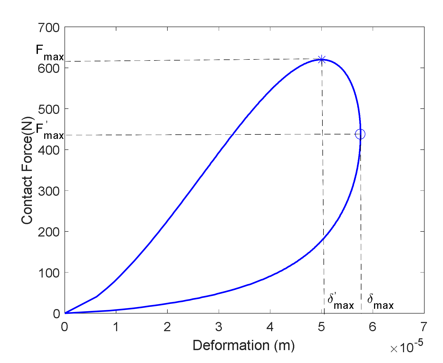
However, different from the basic Hertz model, in which the maximum contact force occurs at the maximum deformation, the calculation of the maximum contact force of the Hertz damping model is more complex. Figure 3 shows the curve of the contact force with respect to deformation, where $M_{\mathrm{ie}}=1 \mathrm{kg}, K={10}^9\mathrm{N}/{\mathrm{m}}^{1.5}, {\dot{\delta }}^{(-)}=0.2\mathrm{m}/\mathrm{s}, \mathrm{and} c_{\mathrm{r}}=0.5,$ and the Gonthier et al., model of the hysteresis damping factor is adopted. The marker “$\ast$” represents the maximum-contact-force point with coordinates (${{\delta }^{\prime }}_{\max }^{}$,$F_{\max }^{}$), and the marker “o” represents the maximum-deformation point with coordinates (${\delta }_{\max }^{}$,${F^{\prime }}_{\max }^{}$). It can be seen that the maximum-contact-force and maximum-deformation points are not consistent.

The relative force error between $F_{\max }^{}$ and ${F^{\prime }}_{\max }^{}$ is defined as follows:

$$\xi =\frac{F_{\max }-{F^{\prime }}_{\max }}{F_{\max }}\times 100\%.$$

(21)

It can be seen from Table 1 that the hysteresis damping factors all have the following form:

$$\lambda =f\left(c_{\mathrm{r}}\right)\frac{K}{{\dot{\delta }}^{(-)}},$$

(22)

where $f\left(c_{\mathrm{r}}\right)$ is a general expression with variable $c_{\mathrm{r}}$.

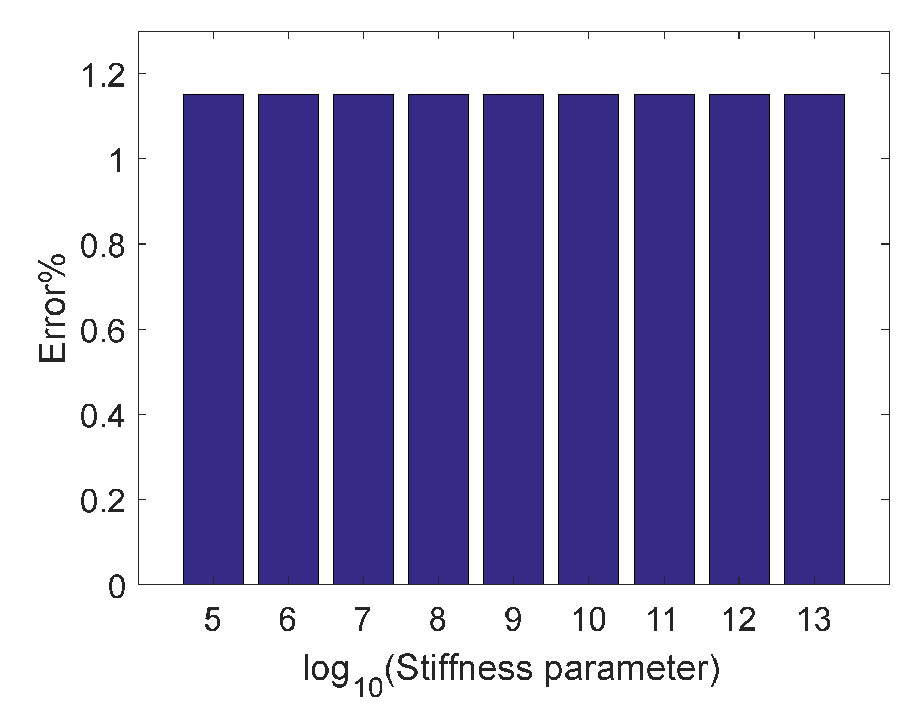
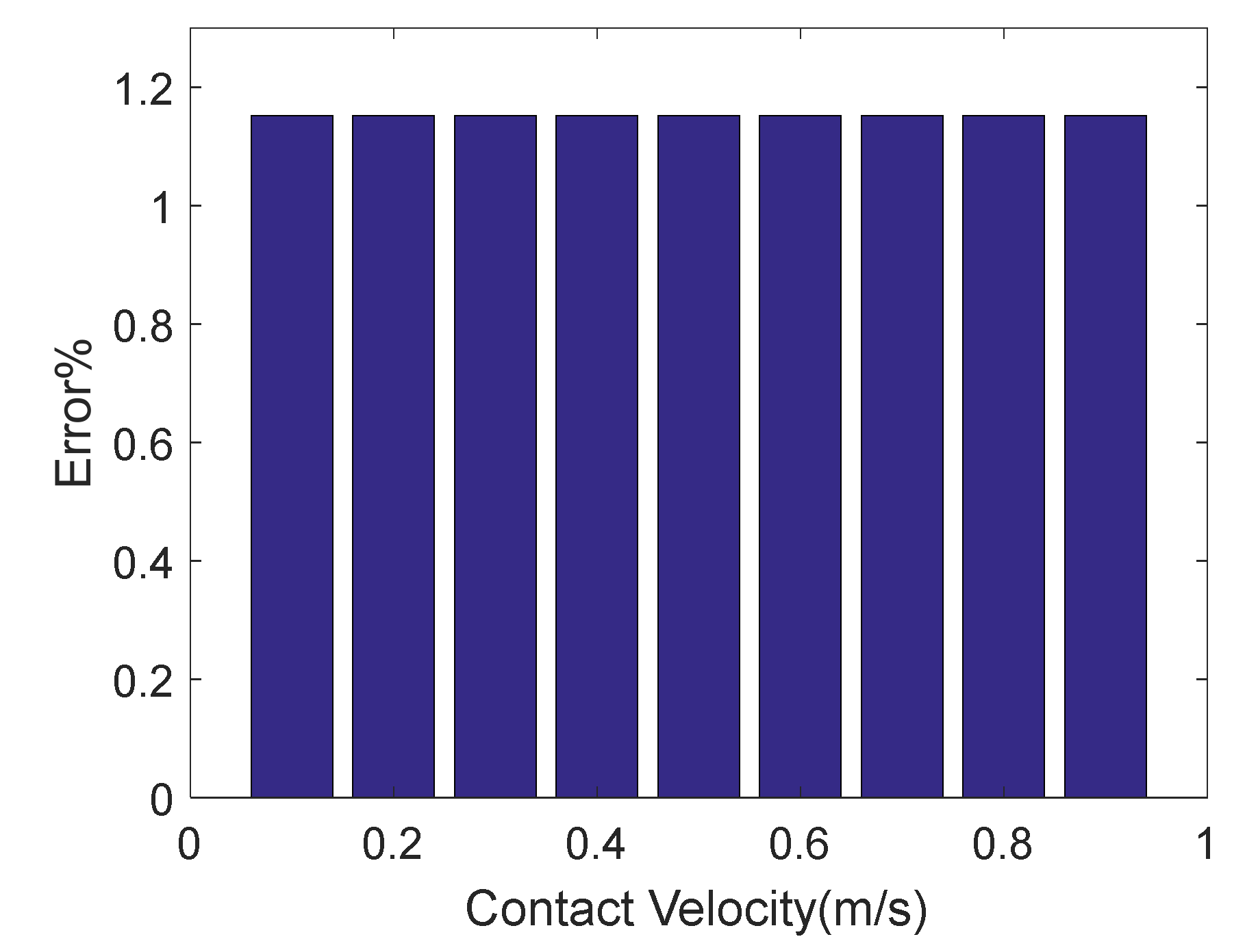
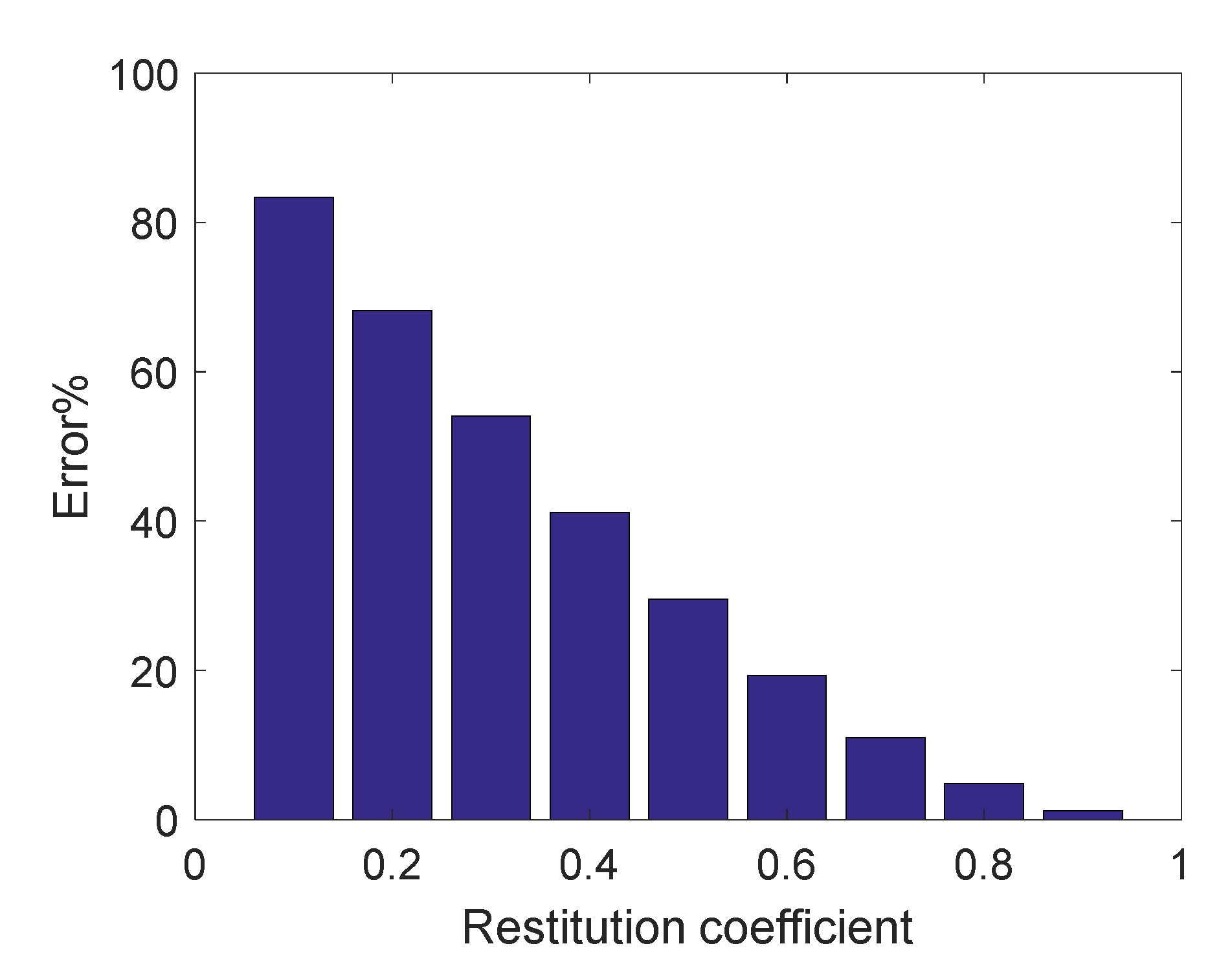
Therefore, assuming that both the kinematics parameters and dynamics parameters of the space robot and target are determined, $\xi$ is only related to the contact stiffness parameter $K$, restitution coefficient $c_{\mathrm{r}}$, and initial relative contact velocity ${\dot{\delta }}^{(-)}$. $\xi$ is proved to be unaffected by $K$ and ${\dot{\delta }}^{(-)}$, as shown in Figure 4 and Figure 5, and becomes increasingly smaller as $c_{\mathrm{r}}$ increases, as shown in Figure 6.

Based on the above analysis, when the restitution coefficient $c_{\mathrm{r}}$ of the contact environment is large enough, $F_{\max }$ can be approximated by ${F^{\prime }}_{\max }$, namely:

$$F_{\max }={\rm K}{\left(\frac{M_{\mathrm{ie}}\left(\alpha +1\right)}{{\lambda }^2}\left(\lambda {\dot{\delta }}^{(-)}+K\ln \left|\frac{K}{\lambda {\dot{\delta }}^{(-)}+K}\right|\right)\right)}^{\frac{\alpha }{\alpha +1}}.$$

(23)

In addition, when the error $\xi$ could not be ignored $F_{\max }$ can be obtained through the comparison of the contact force during the entire contact period, as shown in Figure 3.

4. Configuration Optimization for Capturing Tumbling Target

The maximum contact force is regarded as an optimization indicator in this section, and it can be further written as follows by substituting Equation (22) into Equation (23):

$$F_{\max }=\zeta {\left(M_{\mathrm{ie}}\right)}^{\frac{\alpha }{\alpha +1}},$$

(24)

where

$$\zeta ={{\rm K}}^{\frac{1}{\alpha +1}}{\left(\frac{\left(\alpha +1\right){\left({\dot{\delta }}^{(-)}\right)}^2}{f^2\left(c_{\mathrm{r}}\right)}\left(f\left(c_{\mathrm{r}}\right)+\ln \left|\frac{1}{f\left(c_{\mathrm{r}}\right)+1}\right|\right)\right)}^{\frac{\alpha }{\alpha +1}}.$$

From Table 1, it is known that $f\left(c_{\mathrm{r}}\right)>0$ as $0<c_{\mathrm{r}}<1$, and thus $\zeta$ becomes

$$\zeta ={{\rm K}}^{\frac{1}{\alpha +1}}{\left(\frac{\left(\alpha +1\right){\left({\dot{\delta }}^{(-)}\right)}^2}{f^2\left(c_{\mathrm{r}}\right)}\left(f\left(c_{\mathrm{r}}\right)+\ln \frac{1}{f\left(c_{\mathrm{r}}\right)+1}\right)\right)}^{\frac{\alpha }{\alpha +1}}.$$

(25)

Letting $h\left(f\left(c_{\mathrm{r}}\right)\right)=f\left(c_{\mathrm{r}}\right)+\ln \frac{1}{f\left(c_{\mathrm{r}}\right)+1}$, its derivative can be calculated as:

$$h^{\prime }\left(f\left(c_{\mathrm{r}}\right)\right)=\frac{f\left(c_{\mathrm{r}}\right)}{f\left(c_{\mathrm{r}}\right)+1}>0\left(f\left(c_{\mathrm{r}}\right)>0\right).$$

(26)

It is proved that $h\left(f\left(c_{\mathrm{r}}\right)\right)$ is an increasing function, and $h\left(f\left(c_{\mathrm{r}}\right)\right)>h\left(0\right)=0$. Therefore, $\zeta$ is a positive constant when the contact parameters $K,c_{\mathrm{r}},\alpha$ and the initial relative contact velocity ${\dot{\delta }}^{(-)}$ are determined.

Taking the derivative of Equation (24), the following equation can be obtained:

$$F_{\max }{}^{\prime }\left(M_{\mathrm{ie}}\right)=\frac{\alpha \zeta }{\alpha +1}{\left(\frac{1}{M_{\mathrm{ie}}}\right)}^{\frac{1}{\alpha +1}}>0,M_{\mathrm{ie}}>0.$$

(27)

Therefore, $F_{\max }$ is an increasing function and a smaller integrated effective mass is safer. Generally, the kinematics parameters and dynamics parameters of the target and space robot are determined. The best way to decrease $M_{\mathrm{ie}}$ is to optimize $m_{\mathrm{e}}$ by regulating the capture configuration. The relationship between integrated effective mass $M_{\mathrm{ie}}$ and the capture configuration $\mathit{\theta }$ can be directly established as:

$$M_{\mathrm{ie}}=g\left(\mathit{\theta }\right),$$

(28)

where $g\left(\mathit{\theta }\right)$ is a general expression with variable $\mathit{\theta }$.

Assuming that, following a specific trajectory in Cartesian space is required in the capture task, a gradient-optimization method in null-space can be used [7,18]. For a free-floating space robot, the relationship between the joint angular velocity and end-effector velocity can be expressed as:

$${\dot{\mathit{x}}}_{\mathrm{e}}={\mathit{J}}_{\mathrm{f}}\dot{\mathit{\theta }},$$

(29)

where ${\mathit{J}}_{\mathrm{f}}$ is the generalized Jacobian matrix of the free-floating space robot.

Non-minimum-norm solutions to Equation (29) based on a Jacobian pseudo-inverse can be written in the general form:

$$\dot{\mathit{\theta }}={\mathit{J}}_{\mathrm{f}}{}^{†}{\dot{\mathit{x}}}_{\mathrm{e}}+\rho \aleph \left({\mathit{J}}_{\mathrm{f}}\right)\mathit{\phi },$$

(30)

where ${\mathit{J}}_{\mathrm{f}}{}^{†}$ is the pseudo-inverse of the Jacobian matrix ${\mathit{J}}_{\mathrm{f}}$. $\aleph \left({\mathit{J}}_{\mathrm{f}}\right)=\mathit{E}-{\mathit{J}}_{\mathrm{f}}{}^{†}{J}_{\mathrm{f}}$ is the null space of ${\mathit{J}}_{\mathrm{f}}$, $\rho$ is a gain coefficient, and $\mathit{\phi }$ is an arbitrary vector that can be designed as:

$$\mathit{\phi }=\left[\frac{\partial g}{\partial {\theta }_1},\frac{\partial g}{\partial {\theta }_2},\cdots ,\frac{\partial g}{\partial {\theta }_n}\right].$$

(31)

Actually, task priority exists in Equation (31), where the desired trajectory following has higher priority and the optimization of the objective function by null-space has lower priority. This ensures that the space robot can first accurately reach the capture point along the preset trajectory, and then try to optimize the objective function as much as possible.

5. Numerical Simulations

5.1. Simulation for a 3-Degree-of-Freedom Free-Floating Space Robot

A 3-degree-of-freedom (3-DOF) free-floating space robot is studied and shown in Figure 7 with a = 0.6 m, b = 1.4 m, c = 1.6 m, and d = 0.5 m. ${\mathit{r}}_{tp}=\left[-0.25, 0.15, 0\right] \mathrm{m}$ and ${\mathit{\omega }}_{\mathrm{t}}=\left[0, 0,2\right] \mathrm{deg}/\mathrm{s}$ are both expressed in the target coordinate frame. The dynamics parameters of the space robot and target are listed in

Table 2. Dynamics parameters of 3-DOF free-floating space robot and the target.

Part	Mass (kg)	Inertia Matrix (kg•m2)
Link 1	5	diag([0.01, 0.82, 0.82])
Link 2	6	diag([0.01, 1.28, 1.28])
Link 3	4	diag([0.00, 0.09, 0.09])
Base	500	diag([200, 200, 200])
Target	200	diag([100, 100, 100])

.

5.1.1. Accuracy of Proposed Maximum-Contact-Force Model for 3-DOF Space Robot

Since the important indicator $F_{\max }$ is obtained from the integrated-effective-mass-based continuous-contact model, its effectiveness must be verified. The contact parameters are set as $\alpha =1.5$, $K={10}^9\mathrm{N}/{\mathrm{m}}^{1.5}$, and $c_{\mathrm{r}}=0.9$, and the Herbert–McWhannell model in Table 1 is chosen as the hysteresis damping factor. The initial state of the target is with position [2.75, 1.45, 0] m, Euler angle [0, 0, 0] deg, angular velocity [0, 0, 2] deg/s, and linear velocity [0, 0, 0] m/s. Ten capture configurations are randomly selected and the classical numerical integration method is used for comparison since it can provide accurate results.

The model accuracy is defined as:

$$\zeta =1-\left|\frac{F_{\max \_model}-F_{\max \_exact}}{F_{\max \_exact}}\right|\times 100\%,$$

(32)

where $F_{\max \_\mathrm{model}}$ is the maximum contact force obtained from the proposed model and $F_{\max \_\mathrm{exact}}$ is that obtained from the classical numerical integration method.

The simulation results in

Table 3. Accuracy of maximum-contact-force model for 3-DOF space robot.

Capture Configuration (Deg)	Integrated Effective Mass (kg)	Proposed Method (kN)	Numerical Integration Method (kN)	Model Accuracy
[36, 30, −4]	1.555	0.834	0.844	98.83%
[85, −41, 11]	1.648	0.863	0.873	98.84%
[−75, 30, 12]	3.679	1.397	1.414	98.86%
[10, 86, −76]	4.299	1.534	1.552	98.85%
[0, 90, −90]	5.817	1.840	1.861	98.84%
[30, 21, −56]	5.926	1.860	1.882	98.84%
[54, −30, −5]	7.446	2.133	2.158	98.87%
[−10, −18, 30]	9.635	2.490	2.519	98.84%
[46, −45, 0]	13.74	3.081	3.119	98.78%
[−6, 20, −7]	21.093	3.985	4.036	98.73%

show that the proposed maximum-contact-force model has good accuracy. In addition, the following conclusions can be confirmed from the table.

I.

Different capture configurations produce different integrated effective masses;

II.

The maximum contact force increases as the integrated effective mass increases;

III.

The optimization of maximum contact force is necessary as its value may vary widely.

5.1.2. Configuration Optimization for 3-DOF Space Robot

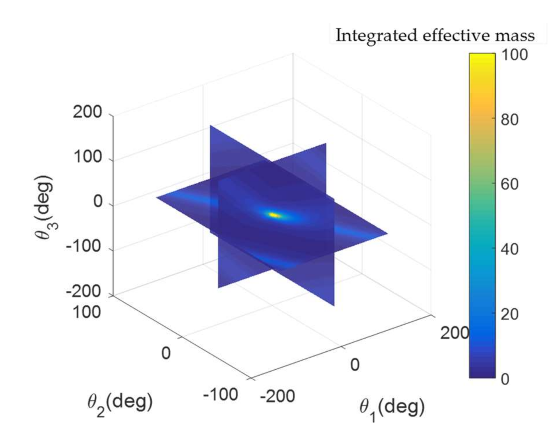
Combining the expression of integrated effective mass, the mapping relationship between the capture configuration and integrated effective mass is shown in Figure 8 with initial relative contact velocity 0.2 m/s, $-90 \mathrm{deg}\le {\theta }_1\le 90 \mathrm{deg},$, $-120 \mathrm{deg}\le {\theta }_2\le 120 \mathrm{deg}$ and $-120 \mathrm{deg}\le {\theta }_3\le 120 \mathrm{deg}$. The color bar shows the integrated effective mass corresponding to different capture configurations of space robot. From the analysis in Section 4, it can be seen that the maximum contact force increases with the increase of integrated effective mass, and thus the capture configuration with small integrated effective mass is preferable on the premise of ensuring the correct capture pose of the end-effector.

Figure 9 depicts the slice map at ${\theta }_1=0 \mathrm{deg}$, ${\theta }_2=0 \mathrm{deg}$, and ${\theta }_3=0 \mathrm{deg}$. It can be seen that the maximum value of integrated effective mass occurs at $\mathit{\theta }=\left[0,0,0\right] \mathrm{deg}$ and it is the exact configuration when the robotic arm is fully deployed. Several researchers proposed to use “straight arm” to capture a target with the purpose of reducing the base disturbance [36]. According to its definition, this fully deployed state is one case of the “straight arm”; however, the space robot and target may suffer a very large contact force as stated above.

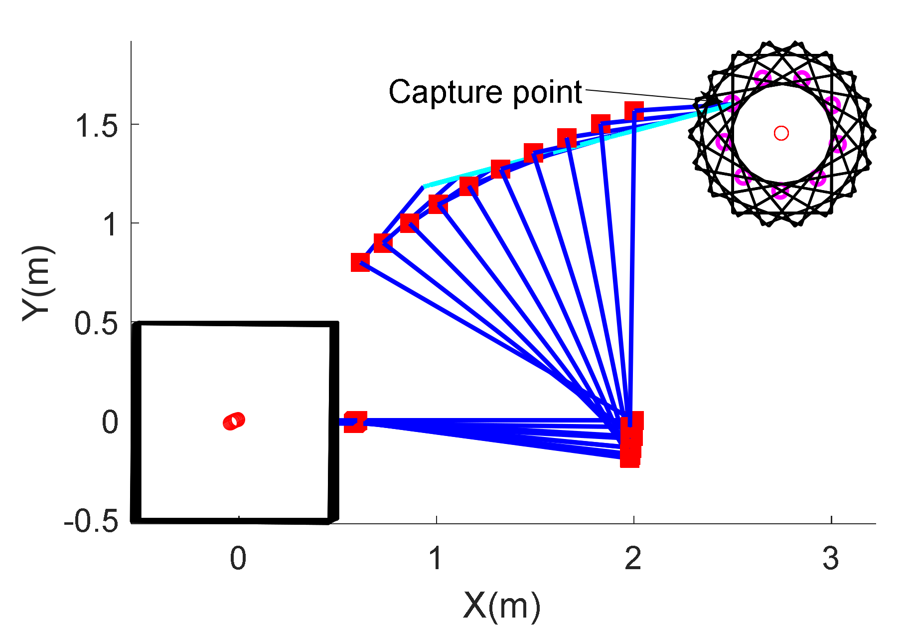
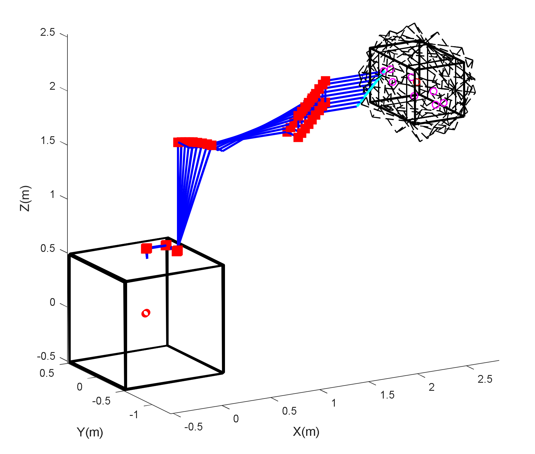
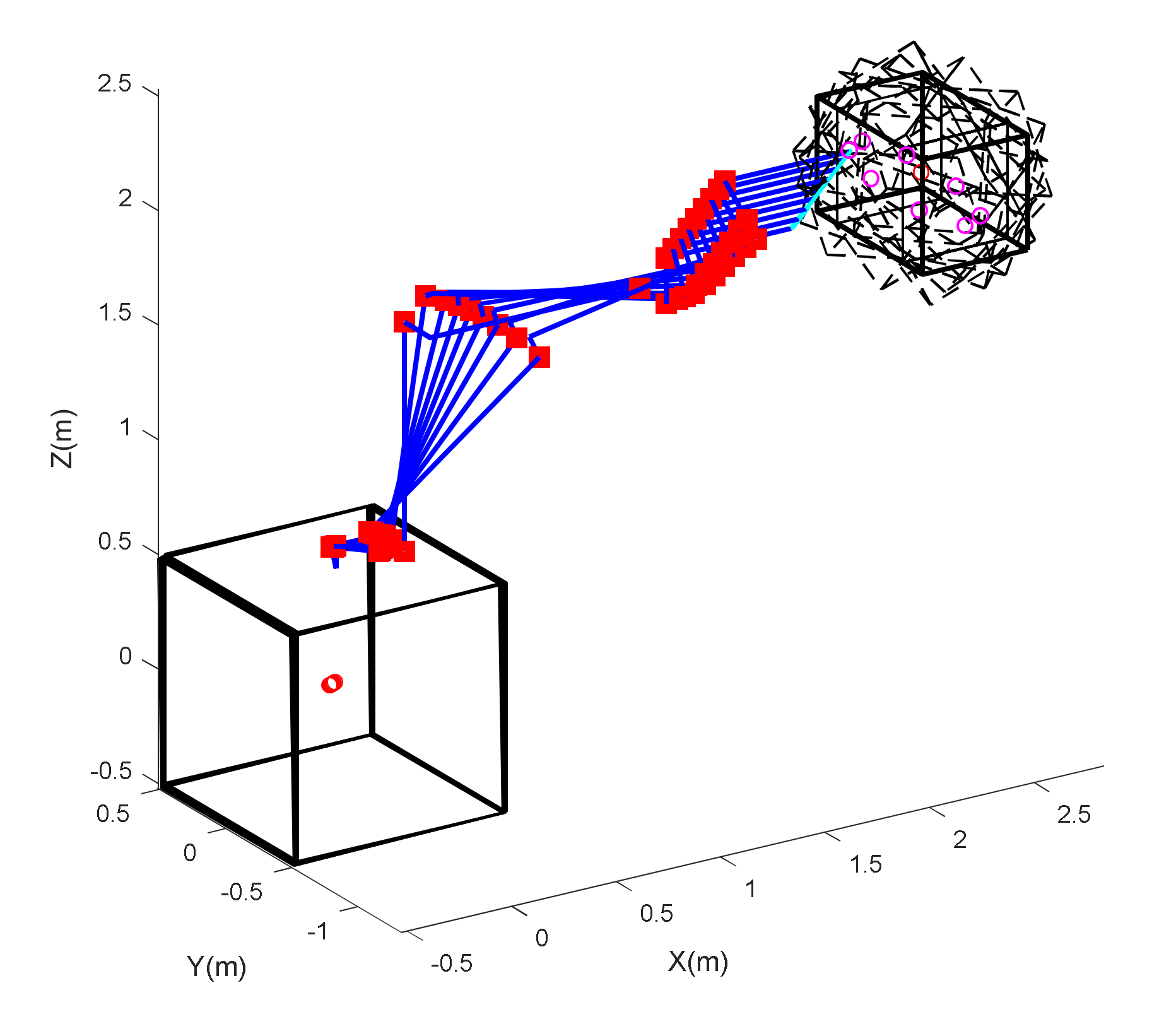
The straight-line trajectory following of the end-effector is assumed to be required in the task, the initial configuration is $\mathit{\theta }=\left[0,150,-100\right] \mathrm{deg}$ and the total task time is 180 s. Figure 10 shows the capture process of a 3-dof space robot without optimization and Figure 11 shows the capture process optimized by the gradient-optimization method in null-space that has been proposed. It can be seen that a space robot can realize the trajectory following and reach the capture point in time in both capture processes, but with different capture configurations. The simulation comparison results are listed in

Table 4. Simulation comparison results of 3-dof space robot.

	Capture Configuration (Deg)	Integrate Effective Mass (kg)	The Maximum Contact Force (kN)
Without optimization	[−2.29, 91.75, −79.77]	5.43	1.71
With optimization	[−16.87, 88.06, 11.33]	1.22	0.72

. Through optimization, the integrated effective mass is decreased by 77.50% and the maximum contact force is decreased by 57.86% accordingly.

The numerical simulation results show the effectiveness of the proposed continuous contact model and the maximum-contact-force indicator for the null-space optimization method. It is worth noting that the reason for choosing a 3-DOF free-floating space robot is to intuitively show the relationship between joint angles and integrated effective mass. In this simulation, the attitude of the space robot end-effector is not considered so that the degrees of freedom of the robot are redundant with respect to the two-dimensional position task constraint. In this way, the null-space optimization method can be implemented. In the actual capture process, the attitude of the space robot end-effector may need to be specified, so a robot with higher degrees of freedom is more suitable, and the optimization method is still applicable as long as the number of degrees of freedom of the robot is redundant with respect to the task constraints.

5.2. Simulation for a 7-Degree-of-Freedom Free-Floating Space Robot

A 7-DOF free-floating space robot is shown in Figure 12 with a = 0.6 m, b = 0.2 m, c = 0.2 m, d = 1.0 m, e = 1.0 m, f = 0.2 m, g = 0.2 m, h = 0.2 m and k = 0.6 m. $r_{tp}=\left[-0.25,0.15,0.1\right] \mathrm{m}$ and ${\mathit{\omega }}_{\mathrm{t}}=\left[1,-0.5,2\right] \mathrm{deg}/\mathrm{s}$ are both expressed in the target coordinate frame. The dynamics parameters of the space robot and target are listed in

Table 5. Dynamics parameters of 7-DOF free-floating space robot and the target.

Part	Mass (kg)	Inertia Matrix (kg•m2)
Link 1	5	diag([0.01, 0.02, 0.02])
Link 2	5	diag([0.02, 0.01, 0.02])
Link 3	10	diag([0.84, 0.01, 0.84])
Link 4	10	diag([0.01, 0.84, 0.84])
Link 5	5	diag([0.02, 0.02, 0.01])
Link 6	5	diag([0.02, 0.02, 0.01])
Link 7	8	diag([0.03, 0.03, 0.01])
Base	1000	diag([500, 500, 500])
Target	200	diag([100, 100, 100])

.

5.2.1. Accuracy of Proposed Maximum-Contact-Force Model for 7-DOF Space Robot

The contact parameters are set as $\alpha =1.5$, $K={10}^9\mathrm{N}/{\mathrm{m}}^{1.5}$, and $c_{\mathrm{r}}=0.9$, and the Herbert–McWhannell model in Table 1 is chosen as the hysteresis damping factor. The initial state of the target is with position [2.3, −0.8, 2] m, Euler angle [0, 0, 0] deg, angular velocity [1, −0.5, 2] deg/s, and linear velocity [0, 0, 0] m/s. Ten capture configurations are randomly selected and the classical numerical integration method is used for comparison. The simulation results in

Table 6. Accuracy of maximum-contact-force model for 7-DOF space robot.

Capture Configuration (Deg)	Integrated Effective Mass (kg)	Proposed Method (kN)	Numerical Integration Method (kN)	Model Accuracy
[0, 29, 54, 10, −10, 120, 32]	4.875	1.664	1.659	99.74%
[10, −2, 160, 0, 33, −5, 80]	7.876	2.218	2.213	99.76%
[55, −22, 45, 11, 36, −10, 160]	2.848	1.205	1.202	99.74%
[−10, 30, 60, −45, 0, 22, 4]	3.061	1.258	1.255	99.76%
[23, 33, −64, 145, 34, 88, 60]	3.167	1.284	1.281	99.76%
[74, −20, 2, 19, 112, 75, −10]	5.003	1.690	1.686	99.76%
[5, 100, 26, −69, 20, 108, −66]	2.513	1.118	1.115	99.75%
[100, 23, 126, −6, 34, 34, −1]	1.658	0.871	0.869	99.76%
[1, 110, −90, 90, 14, 150, 45]	2.677	1.161	1.158	99.75%
[−36, 88, 46, 123, −110, 15, 0]	1.495	0.819	0.817	99.77%

show that the proposed maximum-contact-force model also has high accuracy for a 7-DOF space robot.

5.2.2. Configuration Optimization for 7-DOF Space Robot

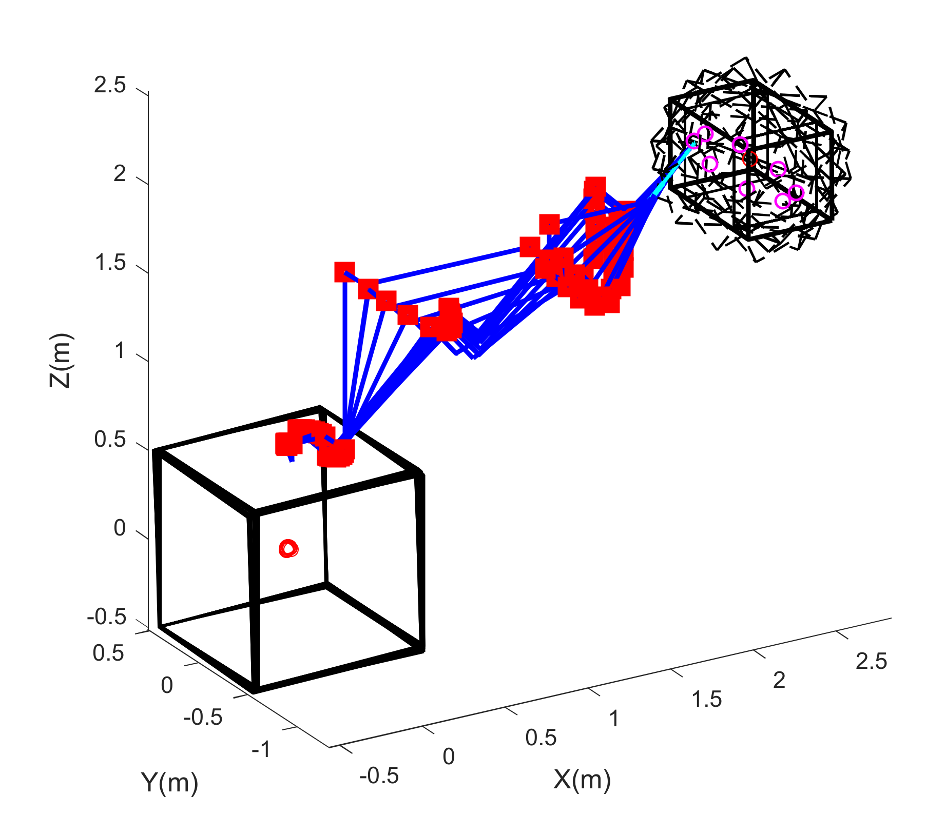
The straight-line trajectory following of the end-effector is assumed to be required in the task, the initial configuration is $\mathit{\theta }=\left[0,90, 90,-90,90,90, 0\right] \mathrm{deg}$, and the total task time is 157 s. Figure 13 shows the capture process of a 7-dof space robot without optimization, Figure 14 shows the capture process with maximum-contact-force optimization and the constraint of specified pose of the end-effector, and Figure 15 shows the capture process with maximum-contact-force optimization and the constraint of specified position of the end-effector. The simulation comparison results are listed in

Table 7. Simulation comparison results of 7-dof space robot.

	Capture Configuration (Deg)	Integrate Effective Mass (kg)	The Maximum Contact Force (kN)
Without optimization	[−0.81, 90.80, 68.96, −47.37, 67.83, 91.01, −0.92]	17.24	3.55
With optimization (Specified pose of the end-effector)	[−47.56, 44.57, 55.96, −24.88, 96.29, 121.85, 56.33]	15.88	3.38
With optimization (Specified position of the end-effector)	[43.84, 127.47, 69.31, −22.02, 121.81, 86.01, 0]	2.70	1.17

. For the case with end-effector pose constraint in the trajectory tracking process, only one degree of freedom can be used to optimize the maximum contact force; the integrated effective mass is decreased by 7.89% and the maximum contact force is decreased by 4.79% accordingly. For the case with only end-effector position constraint in the trajectory tracking process, the integrated effective mass is decreased by 84.34% and the maximum contact force is decreased by 67.04% accordingly. Therefore, for high-degree-of-freedom space robots, additional constraints can be reduced as much as possible during the capture process to provide enough degrees of freedom to optimize the maximum contact force.

6. Conclusions

Taking the maximum contact force as an indicator, the capture configuration of a free-floating space robot capturing a tumbling target is optimized in this paper. The concept of integrated effective mass is first proposed, and a general continuous contact model that is also suitable for non-central collisions is given. Simulation results verified that the maximum contact force can be effectively reduced by optimizing the capture configuration. However, it is worth noting that the maximum-contact-force expression proposed is more suitable for the case in which the contact environment exhibits a high restitution coefficient. For the contact problem with a low restitution coefficient, the maximum contact force can be obtained through the comparison of the contact force during the entire contact period by virtue of the proposed continuous contact model. Due to the large error of the maximum contact force model for the low restitution coefficient environment as mentioned in Section 3, it is not recommended to use the null-space optimization method. Algorithms such as PSO can be used to optimize the numerical solution of the maximum contact force.

References

- Liu, H.; Liu, D.Y.; Jiang, Z.N. Review and Prospect of Space Manipulator Technology. Hangkong Xuebao 2021, 42, 524164. [Google Scholar]
- Flores-Abad, A.; Ma, O.; Pham, K.; Ulrich, S. A Review of Space Robotics Technologies for On-orbit Servicing. Prog. Aerosp. Sci. 2014, 68, 1–26. [Google Scholar] [CrossRef] [Green Version]
- Pan, G.; Jia, Q.; Chen, G.; Li, T.; Liu, C. A Control Method of Space Manipulator for Peg-in-Hole Assembly Task Considering Equivalent Stiffness Optimization. Aerospace 2021, 8, 310. [Google Scholar] [CrossRef]
- Li, Z.; Wang, B.; Liu, H. Target Capturing Control for Space Robots with Unknown Mass Properties: A Self-Tuning Method Based on Gyros and Cameras. Sensors 2016, 16, 1383. [Google Scholar] [CrossRef] [PubMed] [Green Version]
- Sun, Y.; Wang, Q.; Liu, Y.; Xie, Z.; Jin, M.; Liu, H. A Survey of Non-cooperative Target Capturing Methods. Guofang Keji Daxue Xuebao 2020, 42, 74–90. [Google Scholar]
- Stolfi, A.; Gasbarri, P.; Sabatini, M. A Parametric Analysis of a Controlled Deployable Space Manipulator for Capturing a Non-cooperative Flexible Satellite. Acta Astronaut. 2018, 148, 317–326. [Google Scholar] [CrossRef]
- Zhang, L.; Jia, Q.; Chen, G.; Sun, H. Pre-impact Trajectory Planning for Minimizing Base Attitude Disturbance in Space Manipulator Systems for a Capture Task. Chin. J. Aeronaut. 2015, 28, 1199–1208. [Google Scholar] [CrossRef] [Green Version]
- Yoshida, K.; Sashida, N. Modeling of Impact Dynamics and Impulse Minimization for Space Robots. In Proceedings of the 1993 IEEE/RSJ International Conference on Intelligent Robots and Systems, Yokohama, Japan, 26–30 July 1993; pp. 2064–2069. [Google Scholar]
- Flores-Abad, A.; Wei, Z.; Ma, O.; Pham, K. Optimal Control of Space Robots for Capturing a Tumbling Object with Uncertainties. J. Guid. Control Dyn. 2014, 37, 2014–2017. [Google Scholar] [CrossRef]
- Liu, Y.; Du, Z.; Wu, Z.; Liu, F.; Li, X. Multiobjective Preimpact Trajectory Planning of Space Manipulator for Self-assembling a Heavy Payload. Int. J. Adv. Rob. Syst. 2021, 18, 17298806. [Google Scholar] [CrossRef]
- James, F.; Shah, S.; Singh, A.; Krishna, K.; Misra, A. Reactionless Maneuvering of a Space Robot in Precapture Phase. J. Guid. Control Dyn. 2016, 39, 2417–2423. [Google Scholar] [CrossRef]
- Xu, W.; Hu, Z.; Yan, L.; Yuan, H.; Liang, B. Modeling and Planning of a Space Robot for Capturing Tumbling Target by Approaching the Dynamic Closest Point. Multibody Syst. Dyn. 2019, 74, 203–241. [Google Scholar] [CrossRef]
- Huang, P.; Wang, M.; Meng, Z.; Zhang, F.; Liu, Z. Attitude Takeover Control for Post-capture of Target Spacecraft using Space Robot. Aerosp. Sci. Technol. 2016, 51, 171–180. [Google Scholar] [CrossRef]
- Wang, M.; Luo, J.; Wang, J.; Yuan, J. Detumbling Strategy and Impedance Control for Space Robot after Capturing an Uncooperative Satellite. Jiqiren 2018, 40, 750–761. [Google Scholar]
- Gangapersaud, R.; Liu, G.; Ruiter, A. Detumbling of a Non-cooperative Target with Unknown Inertial Parameters using a Space Robot. Adv. Space Res. 2019, 63, 3900–3915. [Google Scholar] [CrossRef]
- Chen, G.; Wang, Y.; Wang, Y.; Liang, J.; Zhang, L.; Pan, G. Detumbling Strategy based on Friction Control of Dual-arm Space Robot for Capturing Tumbling Target. Chin. J. Aeronaut. 2020, 33, 1093–1106. [Google Scholar] [CrossRef]
- Wee, L.; Walker, M. On the Dynamics of Contact between Space Robots and Configuration Control for Impact Minimization. IEEE Trans. Robot. Autom. 1993, 9, 581–591. [Google Scholar]
- Yoshida, K.; Dragomir, N. Space Robot Impact Analysis and Satellite-Base Impulse Minimization Using Reaction Null-Space. In Proceedings of the IEEE International Conference on Robotics and Automation, Nagoya, Japan, 21–27 May 1995; pp. 1271–1277. [Google Scholar]
- Nenchev, D.; Yoshida, K. Impact Analysis and Post-Impact Motion Control Issues of a Free-Floating Space Robot Subject to a Force Impulse. IEEE Trans. Robot. Autom. 1999, 15, 548–557. [Google Scholar] [CrossRef]
- Huang, P.; Xu, Y.; Liang, B. Contact and Impact Dynamics of Space Manipulator and Free-flying Target. In Proceedings of the 2005 IEEE/RSJ International Conference on Intelligent Robots and Systems, Edmonton, AB, Canada, 2–6 August 2005; pp. 1935–1940. [Google Scholar]
- Zhang, L.; Jia, Q.; Chen, G.; Sun, H. The Precollision Trajectory Planning of Redundant Space Manipulator for Capture Task. Adv. Mech. Eng. 2014, 2014, 1–10. [Google Scholar] [CrossRef]
- Xie, R.; Kong, X.; Shi, P.; Zhao, Y. Impact Analysis of Space Manipulators During Target Capture. Comput. Simul. 2016, 33, 438–441. [Google Scholar]
- Luka, S.; Janko, S.; Miha, B. A Review of Continuous Contact-force Models in Multibody Dynamics. Int. J. Mech. Sci. 2018, 145, 171–187. [Google Scholar]
- Machado, M.; Moreira, P.; Flores, P.; Lankarani, H. Compliant Contact Force Models in Multibody Dynamics: Evolution of the Hertz Contact Theory. Mech. Mach. Theory 2012, 53, 99–121. [Google Scholar] [CrossRef]
- Zhang, J.; Li, W.; Zhao, L.; He, G. A Continuous Contact Force Model for Impact Analysis in Multibody Dynamics. Mech. Mach. Theory 2020, 153, 103946. [Google Scholar] [CrossRef]
- Yoshikawa, S.; Katsuhiko, Y. Dynamics Evaluation for Capturing a Target by a Space Robot. J. Robot. Soc. Jpn. 1997, 15, 1034–1042. [Google Scholar] [CrossRef]
- Ji, H.; Li, M.; Wang, X.; Li, Y.; Dou, L. Contact-impact Dynamics Simulation for Space Manipulator using Equivalent Spring-damping Model. In Proceedings of the World Congress on Intelligent Control and Automation, Shenyang, China, 29 June–4 July 2014; pp. 3186–3191. [Google Scholar]
- Wu, S.; Mou, F.; Liu, Q.; Cheng, J. Contact Dynamics and Control of a Space Robot Capturing a Tumbling Object. Acta Astronaut. 2018, 151, 532–542. [Google Scholar] [CrossRef]
- She, Y.; Li, S.; Hu, J. Contact Dynamics and Relative Motion Estimation of Non-cooperative Target with Unilateral Contact Constraint. Aerosp. Sci. Technol. 2020, 98, 105705. [Google Scholar] [CrossRef]
- Yoshida, K.; Sashida, N.; Kurazume, R.; Umetani, Y. Modeling of Collision Dynamics for Space Free-Floating Links with Extended Generalized Inertia Tensor. In Proceedings of the IEEE International Conference on Robotics and Automation, Nice, France, 12–14 May 1992; pp. 899–904. [Google Scholar]
- Jia, Q.; Zhang, L.; Chen, G.; Sun, H. Collision Analysis of Space Manipulator Multi-body System based on Equivalent Mass. Yuhang Xuebao 2015, 36, 1356–1362. [Google Scholar]
- Zhang, L.; Jia, Q.; Chen, G.; Sun, H.; Cao, L. Impact Analysis of Space Manipulator Collision with Soft Environment. In Proceedings of the 9th IEEE Conference on Industrial Electronics and Applications, Hangzhou, China, 9–11 June 2014; pp. 1965–1970. [Google Scholar]
- Chen, G.; Liu, D.; Wang, Y.F.; Jia, Q.; Liu, X. Contact Force Minimization for Space Flexible Manipulators based on Effective Mass. J. Guid. Control Dyn. 2019, 42, 1870–1877. [Google Scholar] [CrossRef]
- Gilardi, G.; Sharf, I. Literature Survey of Contact Dynamics Modelling. Mech. Mach. Theory 2002, 37, 1213–1239. [Google Scholar] [CrossRef]
- Khatib, O. Inertial Properties in Robotic Manipulation. An Object-level Framework. Int. J. Rob. Res. 1995, 14, 19–36. [Google Scholar] [CrossRef]
- Cong, P.; Sun, Z. Pre-impact Configuration Planning for Capture Object of Space Manipulator. In Proceedings of the 2nd International Symposium on Systems and Control in Aerospace and Astronautics, Shenzhen, China, 10–12 December 2008; p. 4776179. [Google Scholar]
Figure 1.
Free-floating space robot capturing a tumbling target.
Figure 2.
Classical numerical integration method for contact force calculation.
Figure 3.
Curve of contact force with respect to deformation.
Figure 4.
Errors with different stiffness parameters ().
Figure 5.
Errors with different initial relative contact velocities ().
Figure 6.
Errors with different restitution coefficients ().
Figure 7.
Three-DOF free-floating space robot capturing tumbling target.
Figure 8.
Relationship between integrated effective mass and capture configuration.
Figure 9.
Slice map at ,
and
.
Figure 10.
Capture process of 3-dof space robot without optimization.
Figure 11.
Capture process of 3-dof space robot with maximum-contact-force optimization.
Figure 12.
Seven-DOF free-floating space robot capturing tumbling target.
Figure 13.
Capture process of 7-dof space robot without optimization.
Figure 14.
Capture process of 7-dof space robot with maximum-contact-force optimization and the constraint of specified pose of the end-effector.
Figure 15.
Capture process of 7-dof space robot with maximum-contact-force optimization and the constraint of specified position of the end-effector.