1. Introduction
Recent studies estimate that as many as 400,000 drones will be providing services in the European airspace by 2050 [
1]. Several geometric CR methods have been developed to implement the tactical separation function for these operations. These methods are capable of guaranteeing separation between aircraft without human intervention. Nevertheless, at the traffic densities envisioned for drone operations, these methods start to suffer from destabilising emergent patterns. Multiactor conflicts and knock-on effects can lead to global patterns that cannot be predicted based on limited man-made rules. Researchers have started employing reinforcement learning (RL) techniques for conflict resolution, which can defend against this multiagent emergent behaviour [
2]. RL can train directly in the environment and adapt directly to the interaction between the agents. In previous work [
3], we compared an RL approach with the geometric state-of-the-art Modified Voltage Potential (MVP) method [
4]. The results showed that the employed RL method was not as efficient as the MVP method in preventing losses of minimum separation (LoSs), at higher traffic densities. Nevertheless, at lower traffic densities, the RL method defended in advance against severe conflicts. The MVP method was not able to resolve these in time, as it initiated the conflict resolution manoeuvre later. This suggests that RL approaches can improve the decisions taken by current geometric CR methods. This hypothesis is explored in this work.
Geometric CR algorithms are typically implemented using predefined, fixed rules (e.g., predefined look-ahead time, and in which direction to move out of the conflict) that are used for all conflict geometries. However, at high traffic densities, each aircraft will face a multitude of conflict geometries for which the same values might not be optimal. For example, in some situations it may be useful to have a larger look-ahead time to defend against future conflicts in advance. In other cases, prioritising short-term conflicts may be necessary to avoid false positives from uncertainties accumulating over time. Similarly, fast climbing actions can prevent conflicts with other aircraft when these occupy a single altitude. Additionally, a speed-only state change may be sufficient to resolve the conflict while preventing the ownship from occupying a larger portion of the airspace. All these decisions are dependent of the conflict geometry. Nevertheless, the number of potential geometry variations are too large for experts to create enough rules to cover them all. However, RL approaches are known for their ability to find optimised solutions in systems with a large number of possible states.
In this study, we propose a Soft Actor–Critic (SAC) model, as created by UC Berkeley [
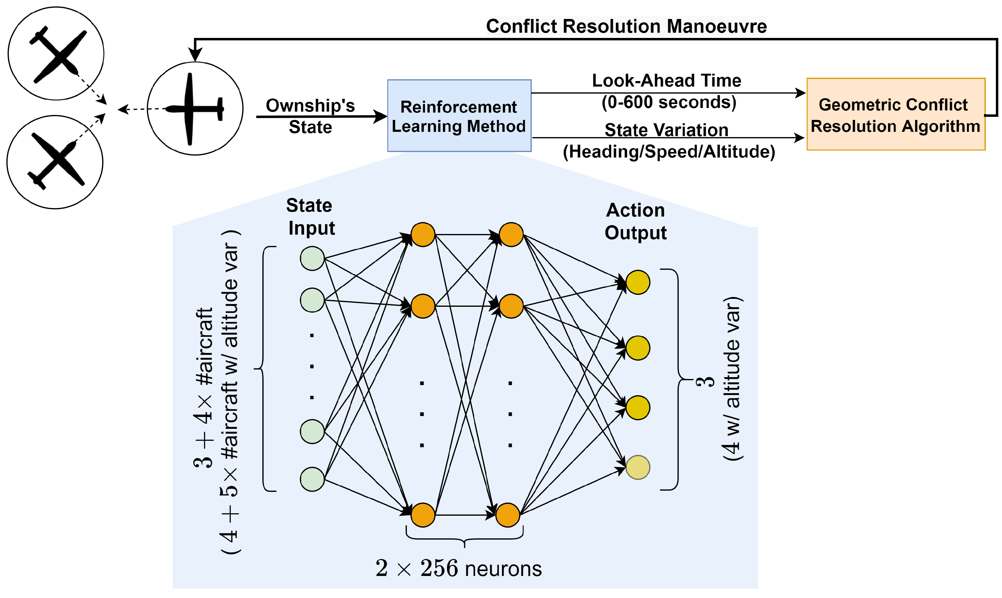
5], that trains within the airspace environment to find the optimal values for the calculation of a conflict resolution manoeuvre. Specifically, in each conflict situation, the RL method defines the look-ahead time (0 s to 600 s) and how many degrees of freedom to employ (i.e, heading, speed, or altitude variation) that the MVP method then uses to generate the CR manoeuvre. The RL method uses the local observations of the aircraft to define these values. This hybrid RL + MVP approach is used for all aircraft involved in the conflict. Finally, experiments are conducted with the open-source, multiagent ATC simulation tool BlueSky [
6]. The source code and scenarios files are available online [
7].
Section 2 introduces the current state-of-the-art research employing RL to improve separation assurance between aircraft. Several works are described, as well as how this paper adds to this body of work.
Section 3 outlines the RL algorithm used in this work, as well as the state, action, and reward formulations used by the RL method.
Section 4 describes the simulation environments of the experiments performed, as well as the conflict detection and resolution (CD&R) methods employed. The hypotheses initially set for the behaviour of hybrid RL + MVP approach are specified in
Section 5.
Section 6 displays the results of the training and the testing phases of the RL method. Finally,
Section 7 and
Section 8 present the discussion and conclusion, respectively.
2. Related Work
The present paper adds to the body of work that uses RL to improve CD&R between aircraft. Recently, an overview of the most recent studies in this area was published [
2], showing that a variety of different RL approaches had been implemented. In previous work, Soltani [
8] used a mixed-integer linear programming (MILP) model to include conflict avoidance in the formulation of taxiing operations planning. Li [
9] developed a deep RL method to compute corrections for an existing collision avoidance approach to account for dense airspace. Henry [
10] employed Q-Learning to find conflict-free sequencing and merging actions. Pham (2019) [
11] used the deep deterministic policy gradient (DDPG) method [
12] for conflict resolution in the presence of surrounding traffic and uncertainty. Isufah (2021) [
13] proposed a multiagent RL (MA-RL) conflict resolution method suitable for promoting cooperation between aircraft. Brittain (2019) [
14] defined an MA-RL method to provide speed advisories to aircraft to avoid conflict in high-density, en route airspace sector. Groot [
15] developed an RL method capable of decreasing the number of intrusions during vertical movements. Dalmau [
16] used message-passing neural networks (MPNN) to allow aircraft to exchange information through a communication protocol before proposing a joint action that promoted flight efficiency and penalised conflicts. Isufah (2002) implemented an algorithm based on graph neural networks where cooperative agents could communicate to jointly generate a resolution manoeuvre [
17]. Brittain (2022) proposed a scalable autonomous separation assurance MA-RL framework for high-density en route airspace sectors with heterogeneous aircraft objectives [
18]. Panoutsakopoulos employed an RL agent for separation assurance of an aircraft with sparse terminal rewards [
19]. Finally, Pham (2022) trained an RL algorithm inspired from Q-learning and DDPG algorithms that can serve as an advisory tool [
20].
All the aforementioned works show that RL has the potential to improve the set of rules used for conflict resolution. RL trains directly in the environment, and can thus adapt to the emergent behaviour resulting from successive avoidance manoeuvres in multiactor conflict situations. However, RL also has its drawbacks, such as nonconvergence, a high dependence on initial conditions, and long training times. We consider that having an RL method that is completely responsible for the definition of avoidance manoeuvres is (practically) infeasible, as it would have severe issues converging to the desirable behaviour. In this paper, we hypothesise that the best usage of RL is, instead, to work towards improving the current performance of state-of-the-art CR methods. We develop a hybrid approach, combining the strengths of geometric methods and learning methods, and hopefully mitigating the drawbacks of each of the individual methods. In this approach, rewards are scaled by the efficacy of the conflict resolution manoeuvres, and the starting point is the current efficacy of the CR method.
3. Improving Conflict Resolution Manoeuvres with Reinforcement Learning
In this work, we employed RL to define the values to input into the CR algorithm responsible for calculating CR manoeuvres. RL was chosen due to its ability to understand and compute a full sequence of actions. A consequence of resolving conflicts is often the creation of secondary conflicts when aircraft move into the path of nearby aircraft while changing their state to resolve a conflict. This often leads to consequent CR manoeuvres to resolve these secondary conflicts. Additionally, knock-on effects of intruders avoiding each other may result in unforeseen trajectory changes. The latter increases uncertainty regarding intruders’ future movements, decreasing the efficacy of CR manoeuvres. RL techniques are often capable of identifying these emerging patterns through direct training in the environment.
Several studies have used other tools such as supervised learning, where classification and regression can be used to estimate the values to be used to aid CR [
21,
22,
23]. These works have shown that these methods can also lead to favourable results. However, these methods do not train directly in the environment, instead resorting to prior knowledge and repeating this knowledge on a large scale. Nevertheless, we assumed no previous knowledge and were mainly interested in the knowledge that RL can learn by adapting to the emergent behaviour experienced in the environment.
Section 3.1 specifies the theoretical background of the RL algorithm employed in this work as well as the defined hyperparameters. Next,
Section 3.2 describes the RL agent employed and how it interacts with the environment.
Section 3.3 details the information that the RL agent receives from the environment, and
Section 3.4 the actions performed by the agent. Finally,
Section 3.5 presents the reward formulation used to evolve the RL agent towards finding optimal actions.
3.1. Learning Algorithm
An RL method consists of an agent interacting with an environment in discrete time steps. At each time step, the agent receives the current state of the environment and performs an action accordingly, for which it receives a reward. An agent’s behaviour is defined by a policy, , which maps states to actions. The goal is to learn a policy which maximizes the reward. Many RL algorithms have been researched in terms of defining the expected reward following an action.
In this work, we used the Soft Actor–Critic (SAC) method as defined in [
5]. SAC is an off-policy actor–critic deep RL algorithm. It employs two different deep neural networks for approximating action-value functions and state-value functions. The actor maps the current state based on the action it estimates to be optimal, while the critic evaluates the action by calculating the value function. The main feature of SAC is its maximum entropy objective, which has practical advantages. The agent is encouraged to explore more widely, which increases the chances of finding optimal behaviour. Second, when the agent finds multiple options for a near-optimal behaviour, the policy commits equal probability to these actions. Studies have found that this improves learning speed [
24].
Table 1 presents the hyperparameters employed in this work. We resorted to two-hidden-layer neural networks with 256 neurons in each layer. Both layers used the rectified linear unit (ReLU) activation function.
3.2. Agent
We employed an RL agent responsible for setting the parameters for the calculation of a CR manoeuvre by a geometric CR method. At each time step, the CR method outputs a new deconflicting state for all aircraft in conflict. The new state aims at preventing LoSs with the necessary minimum path deviation. Every time the CR method computes an avoidance manoeuvre, it uses the following parameters decided by the RL method:
The look-ahead value (between 0 and 600 s).
A selection of which state elements vary (i.e., heading, speed, and/or altitude variation).
The previous values are used by the CR method to generate the CR manoeuvre. The latter is performed by the ownship in order to resolve the conflict and avoid an LoS. Note that all aircraft involved in a CR perform a deconflicting manoeuvre computed by the hybrid RL + CR method.
A single RL agent is considered in this work. Note that several works previously mentioned in
Section 2 have considered the application of MA-RL instead for CR. Looking at the existent body of work [
2], there is no clear preference for either MA-RL or single RL in current studies. The selection of a single agent or multiagent mainly depends on the problem being tackled. Although, theoretically, MA-RL is expected to better handle the nonstationarity of having multiple agents evolving together, a single RL is used in this work for the following reasons:
The single agent can be used on any aircraft; it does not limit the number of aircraft. Instead, MA-RL represents the observations of all agents in its state formulation. As the state array has a fixed size, it can only be used with a fixed number of aircraft.
Through practical experiments, Zhang [
25] concluded that MA learning was weaker than a single agent under the same amount of training. It is thus necessary to balance the optimisation objectives of multiagents in an appropriate way. It is reasonable to expect that MA-RL may require more training due to the increasing state and action formulation, as well as the need to correctly identify which actions had more impact on the reward.
Figure 1 is a high level representation of how the RL agent interacts with the CR algorithm. As per
Figure 1, the state input is transformed into the action output through each layer of the neural network. The compositing of the state and action arrays is described in
Section 3.3 and
Section 3.4, respectively. The variables of the state array have continuous values within the limits presented in
Table 2. The action formulation contains both continuous and discrete values as shown in
Table 3.
3.3. State
The RL method must receive the necessary data for the RL agent to successfully decide which values to input into the CR algorithm for the generation of an effective CR manoeuvre. We took inspiration from the same data that typically distributed, geometric CR methods have access to so as to create a fair comparison. These data included the current state of the ownship aircraft, and the distance, relative heading, and relative altitude of the closest surrounding aircraft. Furthermore, the distance at the closest point of approach (CPA) and the time to the CPA were also considered as this is also information that the CR method has access to. When RL controls altitude variation, on top of heading and speed, it also receives information on the ownship’s current altitude and its relative altitude to the closest intruders.
Table 2 defines the complete state information received by the RL method. Note that the RL method was tested with 2 different implementations of the CR method: (1) the CR method varies heading and speed; (2) the CR method varies heading, speed, and altitude. Thus, the optimal look-ahead times could be related to the level of control that the geometric CR algorithm had over the ownship.
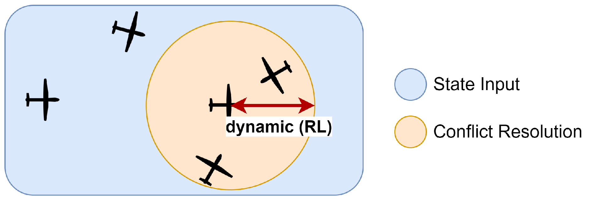
In the state representation, we considered the closest 4 surrounding aircraft. This decision was a balance between giving enough information on the environment, while keeping the state formulation to a minimum size. The size of the problem’s solution grows exponentially with the number of possible states permutations. Thus, this must be limited to guarantee that the RL method trains within an unacceptable amount of time. The 4 closest aircraft (in distance) were chosen in order of their proximity, independently of them being in conflict or not. The reason for considering all aircraft was to allow the RL method to make its decision based not only on the conflicting aircraft but also on nearby nonconflicting aircraft, which could create severe conflicts if they modified their state in the direction of the ownship.
3.4. Action
The RL agent determines the action to be performed for the current state. As previously displayed in
Figure 1, the incoming state values are transformed through each layer of the neural network, in accordance to the neurons’ weights and the activation function in each layer. The output of the final layer must be turned into values that can be used to define the elements of the state of the aircraft that the RL agent controls. All actions were computed using a
tanh activation function; the RL method thus output values between −1 and +1.
Table 3 shows how these values were then translated to the values to be used by the geometric CR method.
The RL method was tested with the geometric CR method controlling (1) heading and speed variations, and (2) heading, speed, and altitude variations. In both cases, the RL method defined the look-ahead value to be used. This was a continuous action. Note that this was the look-ahead time used for resolving conflicts. The RL method received information regarding the aircraft surrounding the ownship through the state input. This was how it “detected” conflicts. Then, it decided on the look-ahead time used for CR, as displayed in
Figure 2. This meant that the method decided which conflicts to consider in the next avoidance manoeuvre. The method could opt, for example, for prioritizing closer conflicts.
Furthermore, depending on the degrees of freedom that the geometric CR algorithm controlled, the RL method defined how the state of the ownship could vary. This selection was a discrete action. For heading, speed, and altitude variation, if the respective value on the state array was higher than 0, the resolution by the geometric CR method included a variation within that degree.
Finally, note that these options took a continuous value (from the RL method’s output) and turned it into a discretised option (≥0 ∨ <0). This could hinder the ability of the RL method to properly understand how its continuous values were used, and limit the efficacy of training. Nevertheless, this was preferred in order to (1) have one RL method responsible for all actions so that the effect of their combination could be directly evaluated by the method, and (2) to have continuous values for the look-ahead time, which allowed the RL method to directly include or disregard specific aircraft in the generation of the avoidance manoeuvre. Future work will explore whether there is an increase in efficiency by having 2 different RL methods. The first may produce continuous actions to define the look-ahead time. The second receives this look-ahead value and outputs discrete actions for the selection/deselection of heading, speed, and altitude variation. Nevertheless, here the first RL method was not aware of the decisions of the second method.
3.5. Reward
The RL method was rewarded at the time step following the one where it set the parameters for the CR manoeuvre calculation for an aircraft. The reward for each state (
) was based on the number of LoSs, as this was the paramount safety objective:
The RL method was not aware of the MVP method, as the latter only contributed indirectly to the reward by attempting to prevent LoSs. Note that efficiency elements could also be added to the reward to decrease flight path and time. Nevertheless, the weight combination of the different elements must be carefully tuned to establish how one LoS compares to a large path deviation. At this phase of this exploratory work, we therefore opted for a simple reward formulation focusing on the main objective.
Furthermore, a reward can be local, when based on the part of the environment that the agent can directly observe, or global, when the reward is based on the global effect on the environment. There are advantages and disadvantages for both types of rewards. On the one hand, local reward may promote “selfish” behaviour as each agent attempts to increase its own reward [
26]. When solving a task in a distributed manner, if each agent tries to optimise its own reward, it may not lead to a globally optimal solution. On the other hand, the task of attributing a global, shared reward from the environment to the agents’ individual actions is often nontrivial since the interactions between the agents and the environment can be highly complex (i.e., the “credit assignment” problem).
In this work, the primary objective was to reduce the total number of LoSs in the airspace. Thus, a global reward was used, where each agent was rewarded based on the total number of LoSs suffered in the airspace. Note that there are technique to (partially) handle the credit assignment problem that were not used in this work. To the best of the authors’ knowledge, these focus mainly in value function decomposition and reward shaping [
27,
28,
29,
30]. However, value function decomposition is hard to apply in off-policy training and potentially suffers from the risk of unbounded divergence [
31]. In our case, we opted for having a simplified reward formulation (see Equation (
1)). Thus, we did not make use of any strategy directed at reducing the credit assignment problem. As a result, however, it was expected that the training phase would take longer, as the RL agent had to explore the state and action spaces at length to understand how its actions influenced the global reward.
4. Experiment: Improving Algorithm Conflict Resolution Manoeuvres with Reinforcement Learning
This section defines the properties of the performed experiment. The latter aimed at using RL to define the values that a distributed, geometric CR method used to generate CR manoeuvres. Note that it was divided into two main phases: training and testing. First, the hybrid RL + CR method was trained continuously with a predefined set of 16 traffic scenarios, at a medium traffic density. Each training scenario ran for 20 min. Afterwards, it was tested with unknown traffic scenarios at different traffic densities. Each testing scenario ran for 30 min. Each traffic density was run with 3 different scenarios, containing different routes. During testing, the performance of the hybrid method was directly compared to the performance of the distributed, geometric CR method, with baseline rules that have been commonly used in other works [
32].
4.1. Flight Routes
The experiment area was a square with an area of 144 NM2. Aircraft were created on the edges of this area, with a minimum spacing equal to the minimum separation distance, to avoid LoSs between spawn aircraft and aircraft arriving at their destination. Aircraft flew a linear route, all at the same altitude. Each linear path was built up of several waypoints. Aircraft were spawned at the same rate as they were deleted from the simulation, in order to maintain the desired traffic density. Naturally, when conflict resolution was applied to the environment, the instantaneous traffic density could be higher than expected as aircraft would take longer to finish their path due to path deviations to avoid LoSs. In order to prevent aircraft from being incorrectly deleted from the simulation when travelling through the edge of the experiment area, or when leaving the area to resolve a conflict, a larger area was set around the experiment area. An aircraft was removed from the simulation once it left this larger area.
4.2. Apparatus and Aircraft Model
An airspace with unmanned traffic scenarios was built using the Open Air Traffic Simulator Bluesky [
6]. The performance characteristics of the DJI Mavic Pro were used to simulate all vehicles. Here, speed and mass were retrieved from the manufacturer’s data, and common conservative values were assumed for turn rate (max: 15
/s) and acceleration/breaking (
).
4.3. Minimum Separation
Minimum safe separation distance may vary based on the traffic density or the structure of the airspace. For unmanned aviation, a single, commonly used value does not (yet) exist. In this experiment, we chose 50 m for the horizontal separation and 50 ft for the vertical separation.
4.4. Conflict Detection
The experiment employed state-based conflict detection for all conditions. This assumed a linear propagation of the current state of all aircraft involved. Using this approach, the time to CPA (in seconds) was calculated as:
where
is the Cartesian distance vector between the involved aircraft (in metres) and
the vector difference between the velocity vectors of the involved aircraft (in metres per second). The distance between aircraft at the CPA (in metres) was calculated as:
When the separation distance was calculated to be smaller than the specified minimal horizontal spacing, a time interval could be calculated in which separation was lost if no action was taken:
These equations were used to detect conflicts, which were said to occur when , and , where is the radius of the protected zone, or the minimum horizontal separation, and is the specified look-ahead time.
With the baseline CR method, a look-ahead time of 300 s was used. This value was selected as, empirically, it was found to be the most efficient common value for the 16 training scenarios within the simulated environment. This is a larger value than commonly used with unmanned aviation. However, smaller values are often considered in constrained airspace to reduce the amount of false conflicts past the borders of the environment [
33]. Finally, this large look-ahead time should not be used in environments with uncertainty regarding intruders’ current position and future path. Expanding the intruders trajectory that far into the future can result in a great amount of false positive conflicts.
4.5. Conflict Resolution
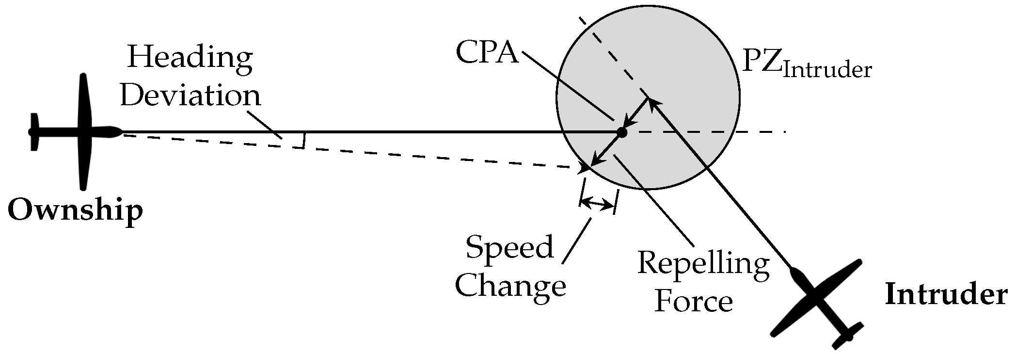
In this work, we used the distributed, geometric CR method MVP. The values used by the MVP method to calculate conflict avoidance manoeuvres were defined by the RL method. The principle of the geometric resolution of the MVP method, as defined by Hoekstra [
4,
34], is displayed in
Figure 3. The MVP method uses the predicted future positions of both ownship and intruder at the CPA. These calculated positions “repel” each other, towards a displacement of the predicted position at the CPA. The avoidance vector is calculated as the vector starting at the future position of the ownship and ending at the edge of the intruder’s protected zone, in the direction of the minimum distance vector. This displacement is thus the shortest way out of the intruder’s protected zone. Dividing the avoidance vector by the time left to the CPA yields a new speed, which can be added to the ownship’s current speed vector resulting in a new advised speed vector. From the latter, a new advised heading and speed can be retrieved. The same principle is used in the vertical situation, resulting in an advised vertical speed. In a multiconflict situation, the final avoidance vector is determined by summing the repulsive forces with all intruders. As it is assumed that both aircraft in a conflict will take (opposite) measures to evade the other, the MVP method is implicitly coordinated.
4.6. Independent Variables
First, two different implementations of the hybrid RL + MVP method were trained with different action formulations. During testing, different traffic densities were introduced to analyse how the RL method performed at traffic densities it was not trained on. Finally, the efficacy of the hybrid RL + MVP was directly compared to that of the baseline MVP method. More details are given below.
4.6.1. Action Formulation
Different action formulations were employed (1) when the CR method only performed heading and speed variations to resolve conflicts and (2) when the geometric CR method used heading, speed, and altitude variation. These allowed direct analyses on how the decisions of the RL method changed depending on the control is had over the state of all aircraft involved in a conflict situation.
4.6.2. Traffic Density
Traffic density varied from low to high according to
Table 4. The RL agent was trained at a medium traffic density, and was then tested with low, medium, and high traffic densities. Thus, it was possible to assess the efficiency of the agent when performing in a traffic density different from that in which it was trained.
4.6.3. Conflict Resolution Manoeuvres
All testing scenarios were run with (1) the hybrid RL + MVP method and (2) the baseline MVP method. The latter used a look-ahead time of 300 s, and moved all aircraft in all available directions. For example, in the case where MVP could vary heading, speed, and altitude, all of these directions were used to resolve the conflict. All aircraft involved in the conflict situation moved in these directions.
4.7. Dependent Variables
Three different categories of measures were used to evaluate the effect of the different operating rules set in the simulation environment: safety, stability, and efficiency.
4.7.1. Safety Analysis
Safety was defined in terms of the total number of conflicts and losses of minimum separation. Fewer conflicts and losses of separation were preferred. Additionally, LoSs were evaluated based on their severity according to how close aircraft got to each other:
Finally, the total time that the aircraft spent resolving conflicts was taken into account.
4.7.2. Stability Analysis
Stability refers to the tendency for tactical conflict avoidance manoeuvres to create secondary conflicts. Aircraft deviate from their straight, nominal path occupying more space in the environment, increasing the likelihood of running into other aircraft. In the literature, this effect has been measured using the domino effect parameter (DEP) [
35]:
where
and
represent the number of conflicts with CD&R
ON and
OFF, respectively. A higher DEP value indicates a more destabilising method, which creates more conflict chain reactions.
4.7.3. Efficiency Analysis
Efficiency was evaluated in terms of the distance travelled and the duration of the flight. Shorter distances and shorter flight duration were preferred.
5. Experiment: Hypotheses
The RL method dictated how far in advance the MVP method initiated a deconflicting manoeuvre, and in which direction(s) each aircraft moved to resolve the conflict. The RL method could adjust its resolution to every conflict geometry. As a result, it was hypothesised that using an RL method to decide the values that the MVP method used for the calculation of the conflict resolution manoeuvres would reduce the total number of LoSs. However, it was also hypothesised that the hybrid RL + MVP method could lose efficiency at traffic densities higher than the one in which it had been trained. Conflict geometries with a higher number of involved aircraft could require different responses from those that the RL learnt.
It was hypothesised that the RL method would make use of a range of look-ahead values, as this could be a powerful way to prioritise short-term conflicts and to defend in advance against potential future severe LoSs. In previous work [
3], an RL method, directed at conflict resolution, chose to defend against several LoSs (i.e., near head-on) in advance. Thus, it was expected that the RL + MVP method would chose larger look-ahead values than the baseline value of 300 s for these kinds of situations. This could increase the number of conflict resolution manoeuvres performed by the hybrid RL + MVP method. Thus, the hybrid RL + MVP solution was expected to have a higher number of conflicts when it used larger look-ahead values.
Finally, the solutions output by the MVP method were implicitly coordinated in pairwise conflicts. It was guaranteed that both aircraft would move in opposite directions. There is no such guarantee in a multiactor conflict. Different aircraft may resolve the conflict by moving in the same direction, making CR manoeuvres ineffective. Nevertheless, in order to reduce LoSs, the RL method had to find some sort of coordination. The RL method could not decide whether the ownship climbed or descended when the altitude was varied; this was calculated by the MVP method. However, it could decide whether the altitude was varied or not. Altitude variation would assuredly move the ownship out of conflict when intruders remained at the same altitude level. Thus, the RL method was expected to employ different combinations of actions, preventing aircraft in a multiactor conflict from attempting to move out of conflict in the same direction.
6. Experiment: Results
As mentioned above, the results section is divided between the training and testing phases. The first shows the evolution of the RL method during the training process. The objective was to reduce the total number of LoSs. In the testing phase, the hybrid RL + MVP method was applied to unknown traffic scenarios. Its performance was directly compared to the baseline MVP method with the same scenarios.
6.1. Training of the Reinforcement Learning Agent
This section shows the evolution of the RL method during training. An episode was a full run of the simulation environment described in
Section 4.1. During training, each episode lasted 20 min. Sixteen different episodes with random flight trajectories and a medium traffic density (see
Section 4.6.2) were created for the training phase. These 16 episodes were run consecutively during training, so it could be evaluated whether the RL method was improving by reducing the number of LoSs for these 16 training scenarios. In total, 150 episodes were run, or roughly nine cycles of the 16 training episodes. For reference, without intervention from the CR method, when aircraft followed their nominal trajectories, the training scenarios had, on average, roughly 1800 conflicts and 600 LoSs.
6.1.1. Safety Analysis
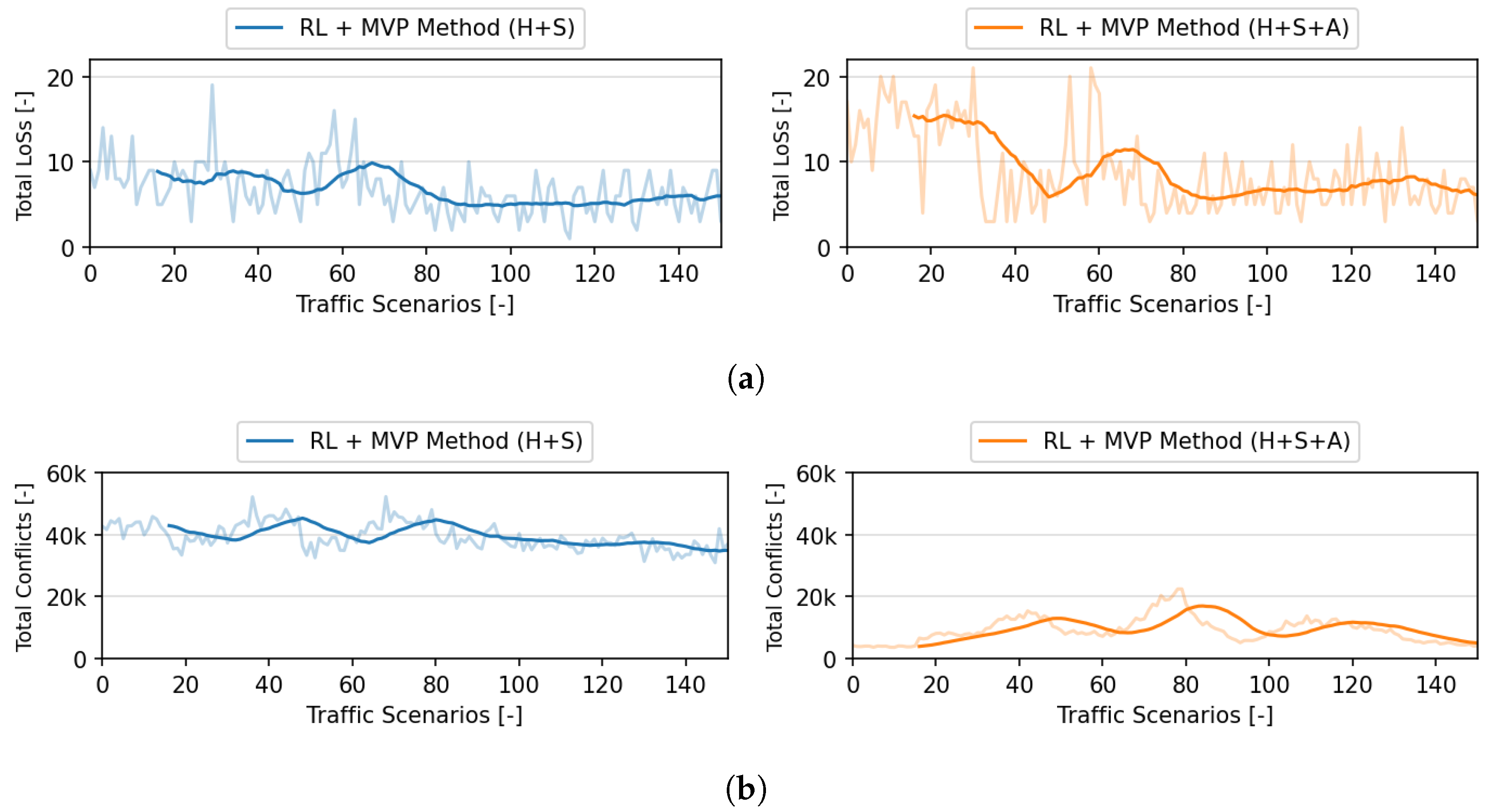
Figure 4 shows the evolution of the RL method for both action formulations in terms of pairwise conflicts and LoSs. A conflict was found once it was identified that two aircraft would be closer than the minimum required separation at a future point in time. Regardless of the number of aircraft involved in a conflict situation, conflicts were counted in pairs. Note that an aircraft could be involved in multiple pairwise conflicts simultaneously. A pairwise conflict was counted only once, independently of its duration.
The values obtained when the hybrid RL + MVP method controlled only heading and speed variations are indicated by “RL + MVP Method (H + S)”. The values with “RL + MVP Method (H + S + A)” indicate the performance when the method controlled altitude variation, on top of heading and speed variations. Both methods converged towards optimal conflict resolution manoeuvres after approximately 90 episodes (see
Figure 4a). They both achieved a comparable number of LoSs. However, “RL + MVP (H + S + A)” did it with considerably fewer conflicts (see
Figure 4b). This was the result of the traffic conditions of the simulated scenarios. As all aircraft were initially set to travel at the same altitude, vertical deviations removed aircraft out of this main layer of traffic, reducing the chance of secondary conflicts.
Table 5 shows the actions performed by the hybrid RL + MVP method at the end of training. Naturally, the exact values used were dependent on the conflict situations that the RL faced. However, the general preference for certain actions was common to all training episodes. When RL + MVP controlled only heading and speed, it strongly favoured performing both heading and speed variations simultaneously (around 99.7% of the total). Moreover, the method favoured speed-only over heading-only actions. Subliminal speed changes can be helpful in resolving conflicts with intruders far away, without the ownship having to occupy a larger amount of airspace. Nevertheless, given that speed-only actions were employed a small number of times (around 0.3% of the total), it was not clear whether the RL method understood this.
When heading, speed, and altitude were controlled, the method opted for either using all degrees of freedom simultaneously or heading and speed only (around 49.8% and 45.4% of the total, respectively). This shows that the RL method found that these two combinations were the most effective manoeuvres with the MVP conflict resolution method. Furthermore, the RL method found it to be advantageous to combine these two manoeuvres. As mentioned in
Section 5, having aircraft in conflict move in different directions can be beneficial for the resolution of the conflict. The conditions in which each combination was employed are developed further in the following sections.
As hypothesised, the RL method used a wide range of look-ahead values. The look-ahead value directly affects when and how the ownship resolves conflicts. On average, the RL method chose a larger look-ahead value than the baseline value of 300 s. Nevertheless, implementing these averages instead of using 300 s did not improve the efficacy of the baseline MVP method. The optimal moment to act against a conflict was highly dependent on the conflict geometry, as shown by the standard deviations of the values generated by the RL method. The RL method selected shorter look-ahead values when altitude was employed. The method learnt to use altitude deviations as a tool to quickly resolve short-term conflicts.
Section 6.1.2 and
Section 6.1.3 further explore the actions of the hybrid RL + MVP method in relation to the state of the environment.
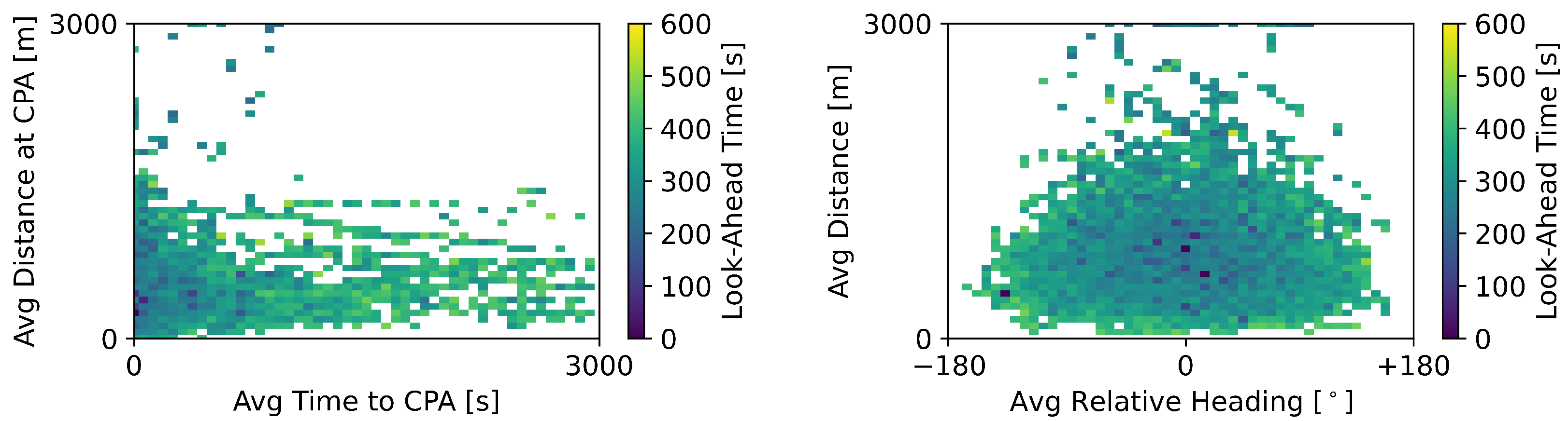
6.1.2. Actions by the Reinforcement Learning Module (Heading + Speed)
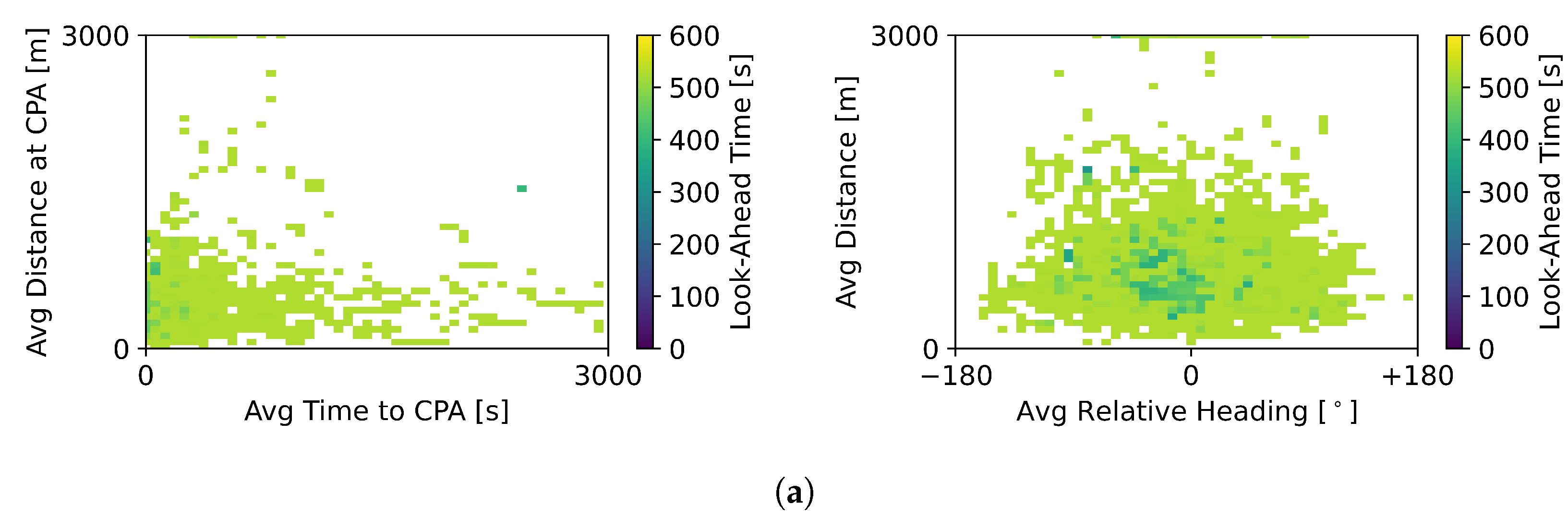
Figure 5 connects some of the data available in the state formulation to the actions chosen by the RL method, which could vary only the heading and speed. The look-ahead time value employed by the RL method in relation to the average distance at the CPA and time to the CPA are shown on the left. The right image displays look-ahead values in relation to the average current distance and average relative bearing.
Figure 5 displays the look-ahead values when both heading and speed variations were used to resolve conflicts. The RL + MVP method had a strong preference for look-ahead values above the baseline value of 300 s, as colour values below 300 s are rare in the graph. Finally, the RL method seemed to prioritise conflicts based on their average time to the CPA and distance at the CPA, as visible from the darker points on the bottom left corner of the left graph.
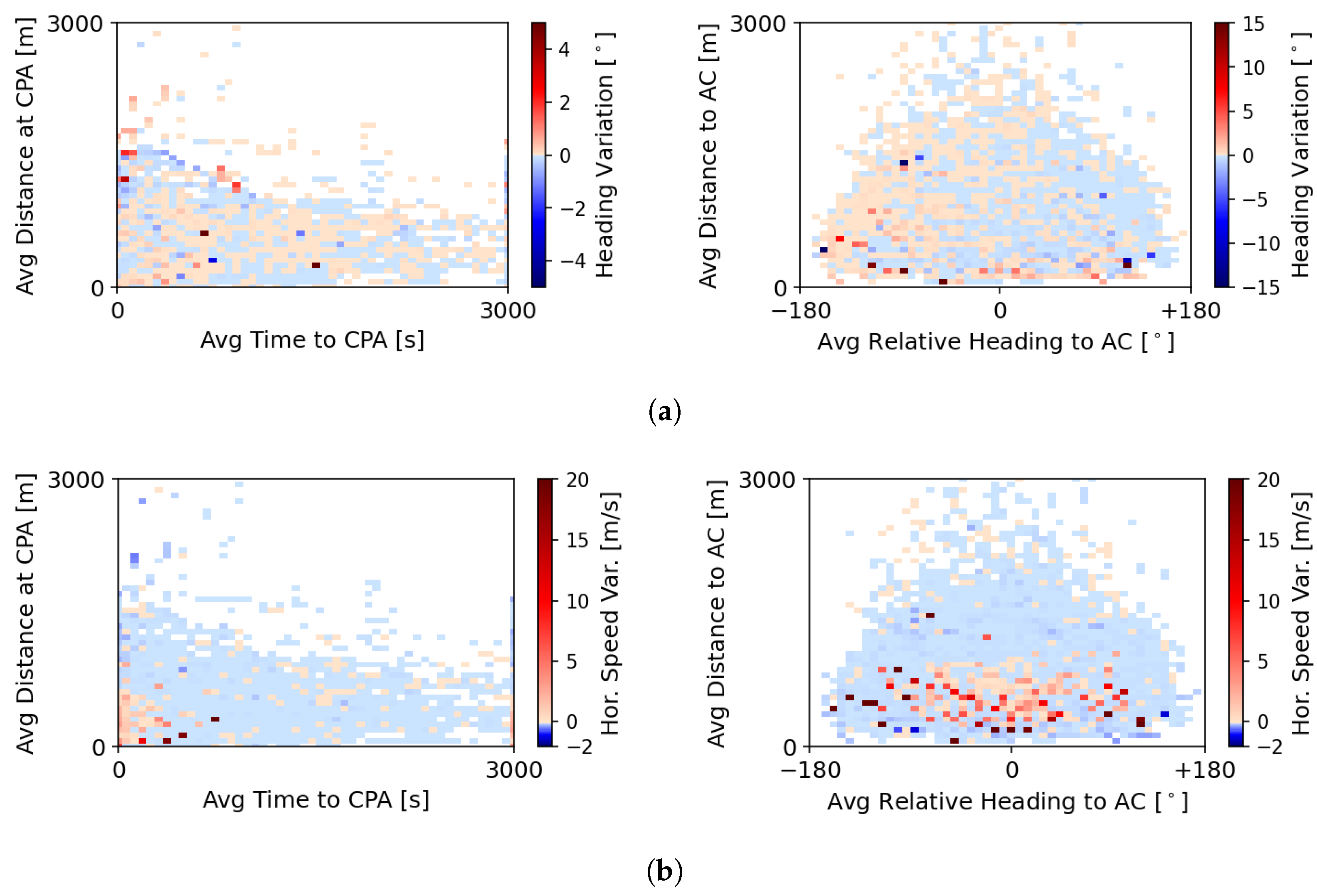
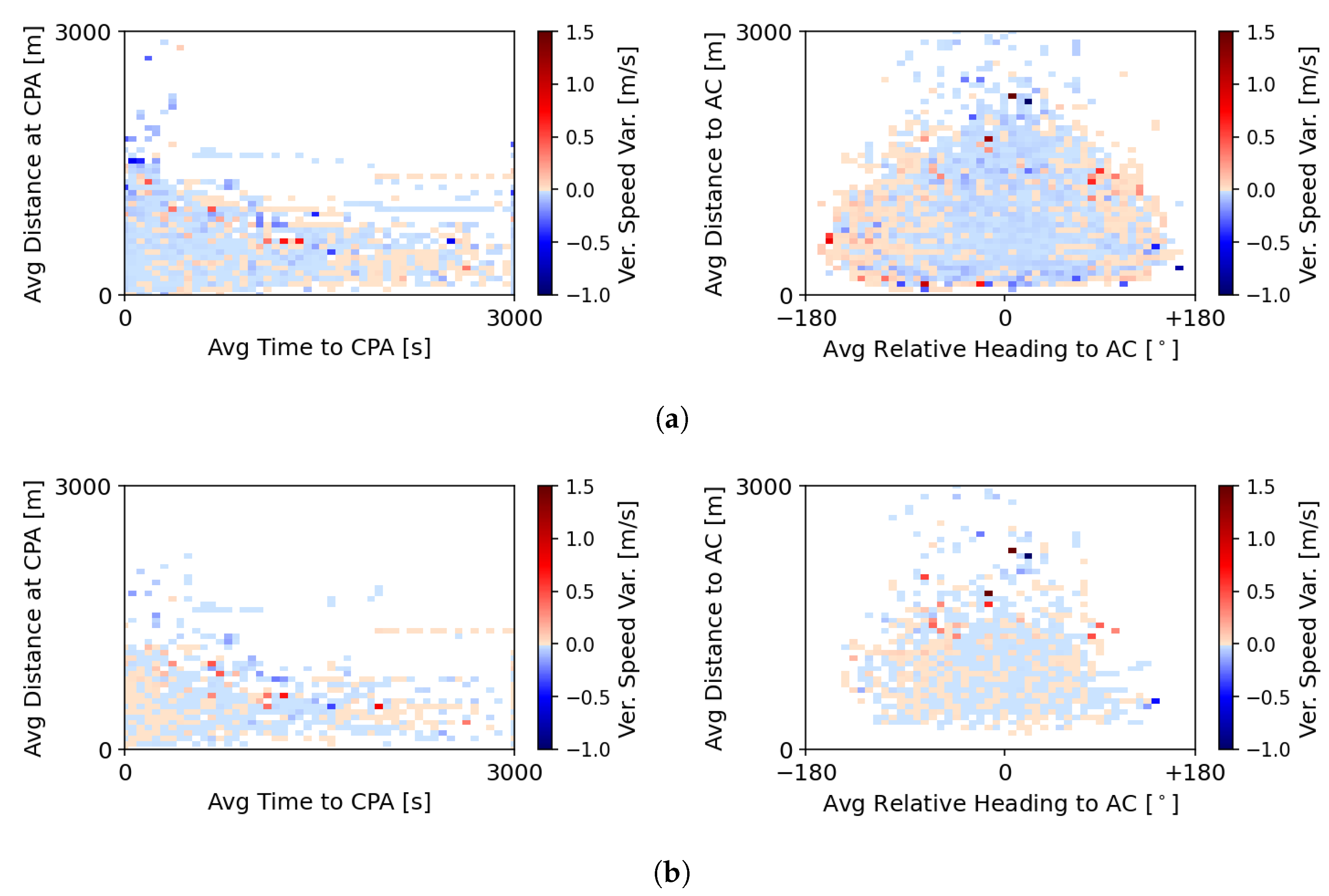
Figure 6 shows the final heading and speed variation of the RL + MVP method for the training episodes. As expected, the heading and speed variations were greater when the surrounding aircraft were closer in distance (see darker points at the bottom of the graphs on the right). The graph to the right of
Figure 6b presents acceleration points (in red) when the surrounding aircraft were closer in distance, and deceleration points (in blue) when aircraft were farther away. When aircraft were closer, the ownship accelerated in order to quickly increase the distance from the surrounding aircraft. When the latter were farther away, the ownship decreased its speed in order to delay the start of the loss of minimum separation. Note, however, that although the CR method output these speeds, it was not guaranteed that the ownship would adopt the final output speed. The adoption of the new deconflicting state was dependent on the performance limits of the ownship.
The results of the baseline MVP method are not shown, as the differences from
Figure 6 are not clearly visible to the naked eye. The use of an RL method to define the parameters that the MVP method used to generate the CR manoeuvre did not greatly change the magnitude of the heading and speed variations performed. However, the RL method impacted the number of intruders considered in the calculation and how far in advance the ownship initiated the CR manoeuvre. For example, when the method selected a longer look-ahead time than the baseline value of 300 s, it initiated CR manoeuvres before the baseline MVP did. In contrast, when the RL method selected lower values, it was both prioritising short-term conflicts and delaying the reaction towards conflicts farther away.
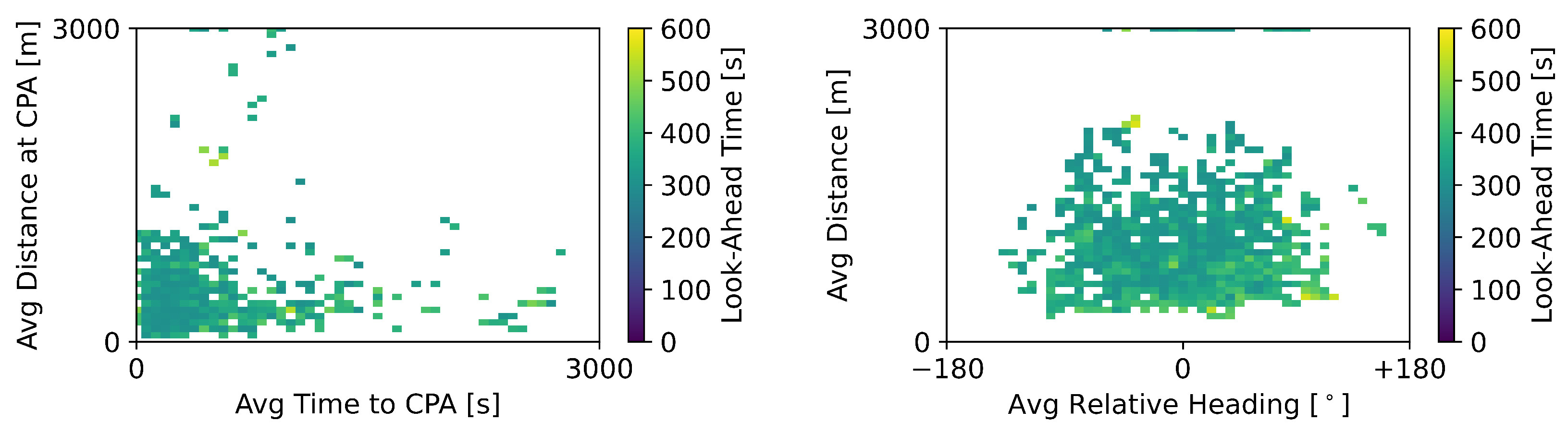
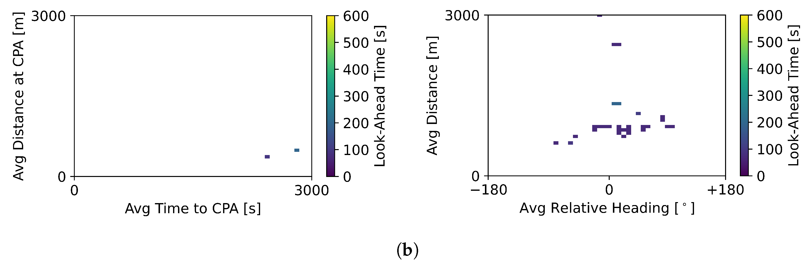
Figure 7 displays the situations for which the RL + MVP method instructed the ownship to defend against a conflict and the baseline MVP method did not. This referred to situations where the RL method output a look-ahead time greater than 300 s. This resulted in the RL + MVP method defending in advance against many conflicts that the baseline MVP would only consider later in time. The graphs show that these intruders were still far away (see graph on the right) and thus would not lead to a LoS situation shortly. Nevertheless, some represented severe LoSs given the small distance at the CPA (see graph on the left).
6.1.3. Actions by the Reinforcement Learning Module (Heading + Speed + Altitude)
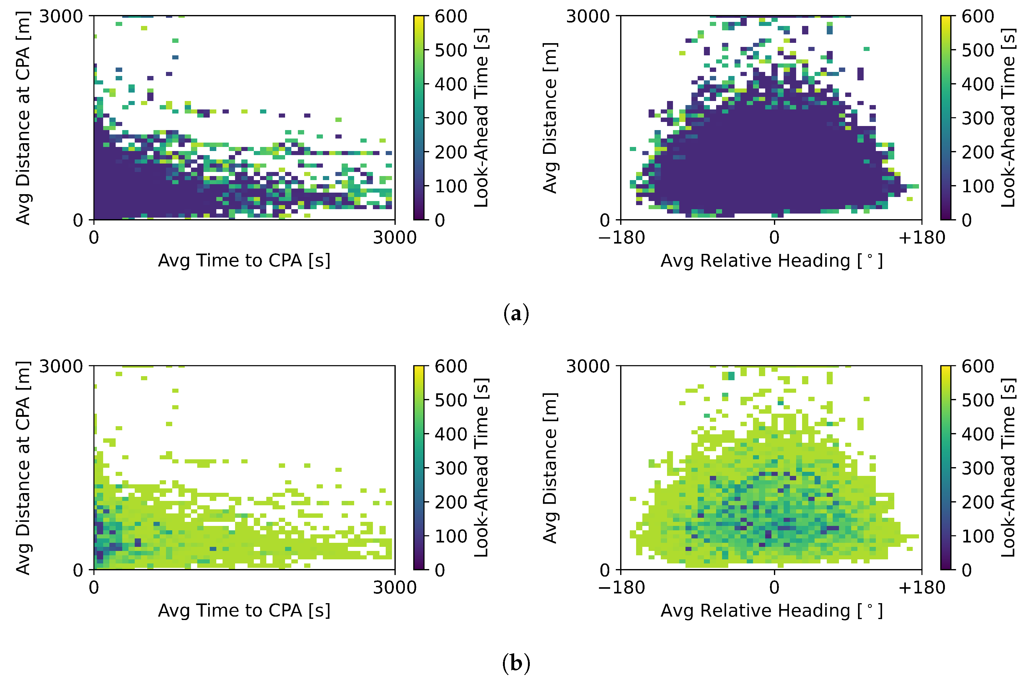
Figure 8 shows the different look-ahead times selected by the RL method depending on the varied degrees of freedom.
Figure 8a displays the look-ahead values produced by the RL method when it varied the heading, speed, and altitude of the ownship to resolve conflicts. Here, it had a preference for look-ahead time values under 200 s (points on the graphs are overwhelming on the darker side of the spectrum representing lower values). As a result, conflicts were resolved later than with the RL method that could only vary heading and speed. This was expected given the extra degree of freedom, i.e., the altitude variation. Since all traffic was set to fly at the same altitude level, vertical deviations were a fast way to resolve a conflict, as the ownship moved away from the main traffic layer.
Figure 8b displays the look-ahead values used for manoeuvres varying only the heading and horizontal speed. Compared to the values shown previously in
Figure 5, the points in the graph here are lighter in colour indicating larger look-ahead values. In this case, the RL method resorted to larger look-ahead values. This is in line with the information displayed in
Table 5.
The direct comparison between
Figure 8a,b show that (1) heading, speed, and altitude deviations were used with short look-ahead time values, and (2) heading and speed variations were used with larger values. Thus, it seemed that the RL method used heading and speed manoeuvres to resolve conflicts with more time in advance and resorted to altitude variation to resolve the remaining short-term conflicts. The prioritisation of short-term conflicts benefits its resolution, as the generated deconflicting manoeuvre was calculated by taking into account only the best solution for these conflicts. Moreover, by having fewer aircraft resolve conflicts in the vertical dimension, when the latter was used, it was more effective, as most of the aircraft were in the main traffic layer.
Figure 9 shows the final heading and speed variation of the hybrid RL + MVP method that could vary the heading, speed, and altitude. Compared to the heading and speed variations performed by the RL method that could only control heading and speed variations (see
Figure 6), stronger speed variations are visible (see darker points at the bottom of the right graph in
Figure 9b). Additionally, based on the average values of
Table 5, this RL method defended against conflicts later than its counterpart that controlled only heading and speed variation. In conclusion, more imminent conflicts required larger state variations to resolve.
Figure 10a,b show the final vertical speed variation for the baseline MVP and the hybrid RL + MVP methods, respectively. There were differences in the number of conflict situations in which the methods employed altitude deviation, as
Figure 10b has fewer data points than
Figure 10a. The baseline MVP method employed headings, speed, and altitude in all conflict situations. However, as previously shown in
Table 5, the hybrid RL + MVP method employed altitude variation in approximately ≈50% of the total conflict situations. Thus, there were fewer occasions with altitude deviation.
Finally, analogously to the method examined in
Section 6.1.2, certain look-ahead values resulted in no defensive action being adopted by the ownship.
Figure 11a shows the situations where the baseline MVP did not perform a deconflicting manoeuvre but the hybrid method RL + MVP did. This was the result of the RL + MVP selecting a longer look-ahead time than the baseline value of 300 s. In turn,
Figure 11b displays the situations for which the hybrid RL + MVP method did not instruct the ownship to initiate conflict resolution, and the baseline MVP method did. Here, the look-ahead values were below 300 s, during which no intruder was found. The hybrid RL + MVP method defended against conflicts more frequently than the baseline MVP method.
6.2. Testing of the Reinforcement Learning Agent
The trained RL + MVP method was then tested with different traffic scenarios at low, medium, and high traffic densities. For each traffic density, three repetitions were run with three different route scenarios, for a total of nine different traffic scenarios. During the testing phase, each scenario was run for 30 min. In both phases, the results of the RL method were compared directly with those of the baseline MVP method.
6.2.1. Safety Analysis
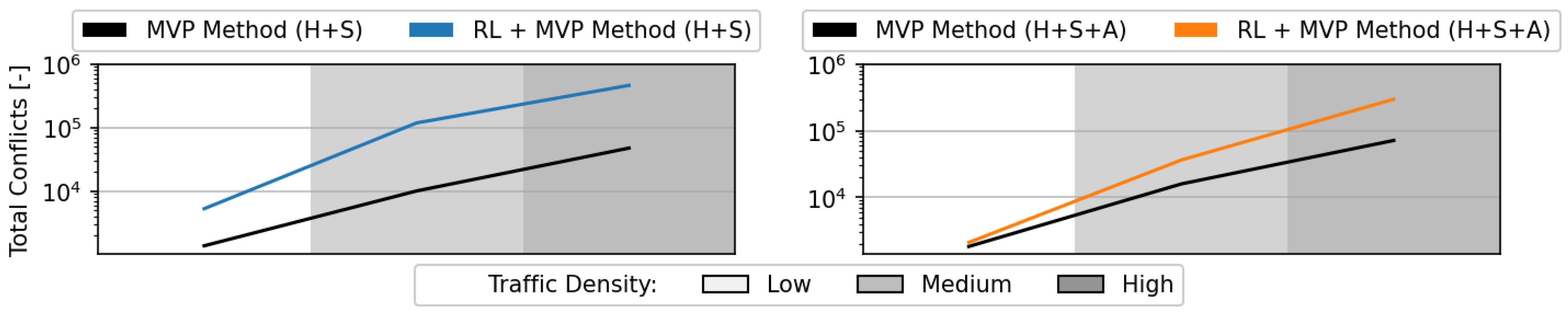
Figure 12 displays the mean total number of pairwise conflicts. A pairwise conflict was counted only once, independently of its duration. Note that this was the number of detected conflicts with a baseline value of 300 s, independent of the final value selected by the RL method, to warrant a direct comparison. Employing the RL method with MVP resulted in a considerably higher number of conflicts than using the baseline MVP method. However, this is not necessarily negative, as previous research has shown that conflicts help spread aircraft within the airspace [
34].
The increase in the total number of conflicts was a direct consequence of the higher number of deconflicting manoeuvres performed by the hybrid RL + MVP method in comparison to the baseline MVP method (see
Figure 7). At high traffic densities, conflict avoidance manoeuvres led to secondary conflicts, as aircraft occupied more airspace by deviating from their nominal, straight path. The increase in the total number of conflicts was less significant when MVP could vary altitude, on top of heading and speed (see graph on the right). This was related to the fact that most aircraft travelled at the same altitude; thus, varying the altitude was less likely to result in secondary conflicts.
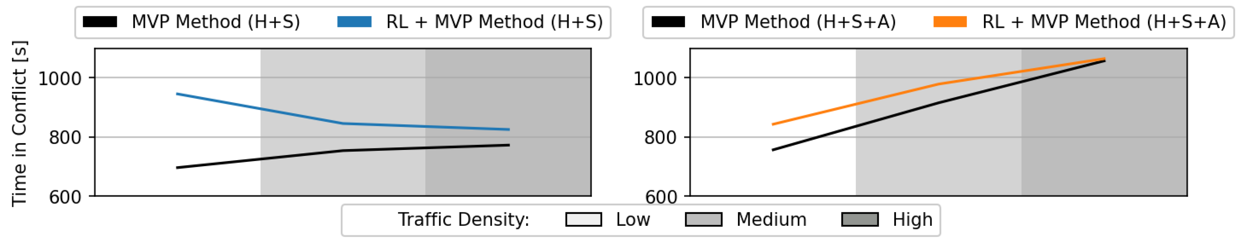
Figure 13 displays the time in conflict per aircraft. An aircraft entered “conflict mode” when it adopted a new state computed by the MVP method. An aircraft exited this mode once it was detected that it was past the previously calculated time to the CPA (and no other conflict was expected between now and the look-ahead time). At this point, the aircraft redirected its course to the next waypoint in its route. The time redirecting towards the next waypoint was not included in the total time spent in conflict.
While aircraft spent more time in conflict with the hybrid RL + MVP method, the increase in time in conflict did not correlate directly with the increase in the total number of conflicts (see
Figure 12). This meant that most conflicts were short in duration and quickly resolved. Additionally, the hybrid RL + MVP method controlling only heading and speed variation (see graph on the left), at the lowest traffic density, had the highest time in conflict, although it had the fewest conflicts. This indicated that the way conflicts were resolved had a greater impact on the total time spent in the conflict.
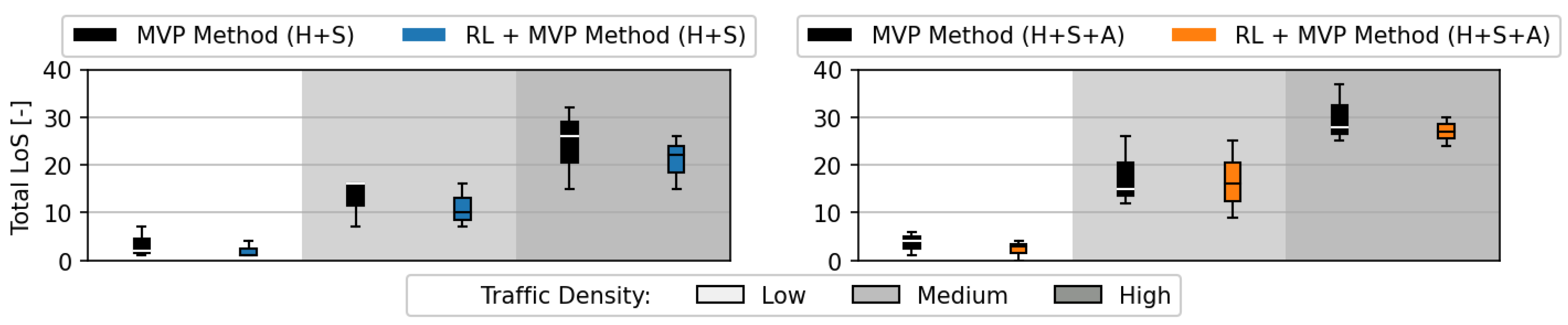
Figure 14 displays the total number of LoS. Reducing the total number of LoSs was the main objective of the RL method. The results show that having the RL method decide the input values for the MVP method led to a reduction of the total number of LoSs on all traffic densities, even at a higher traffic density than the RL method was trained on. This proved that the elements optimised by the RL method, namely, (1) the prioritisation of conflicts depending on the degrees of freedom and (2) the heterogeneity of directions between aircraft in a conflict situation, were common to all traffic densities.
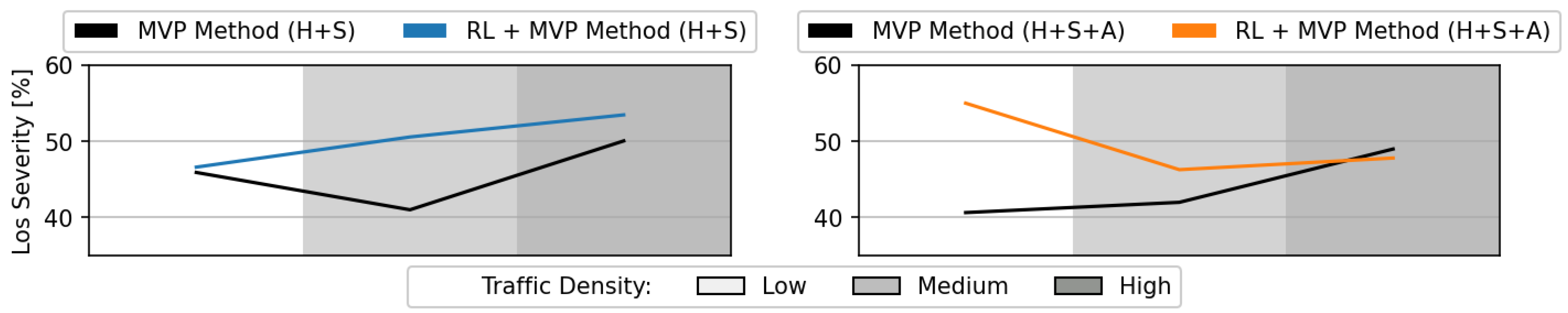
Figure 15 displays the LoS severity. With the hybrid RL + MVP method, the LoS severity was slightly higher, but not to a significant extent. It was likely that the RL + MVP method prevented some of the lowest severity LoSs, leaving out the more severe ones.
6.2.2. Stability Analysis
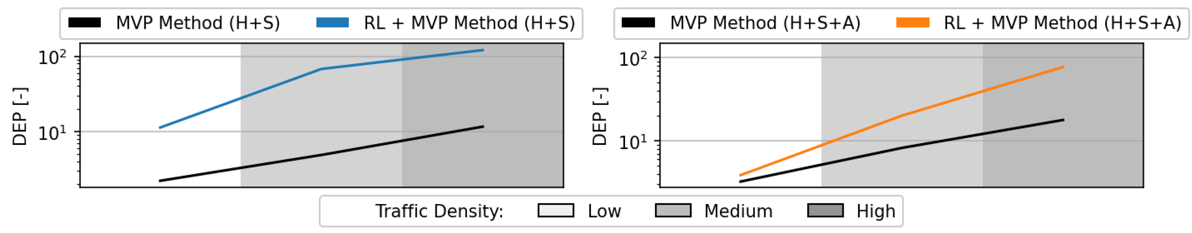
Figure 16 shows the DEP during the testing of the RL method. The increase in DEP was comparable to the increase in the total number of conflicts (see
Figure 12). The increase in the total number of conflicts was a result of a higher number of deconflicting manoeuvres, leading to a higher number of secondary conflicts.
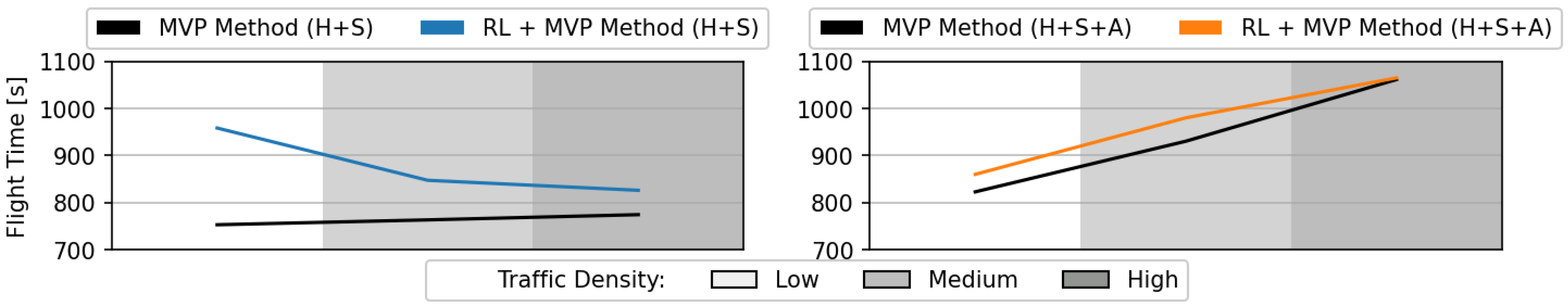
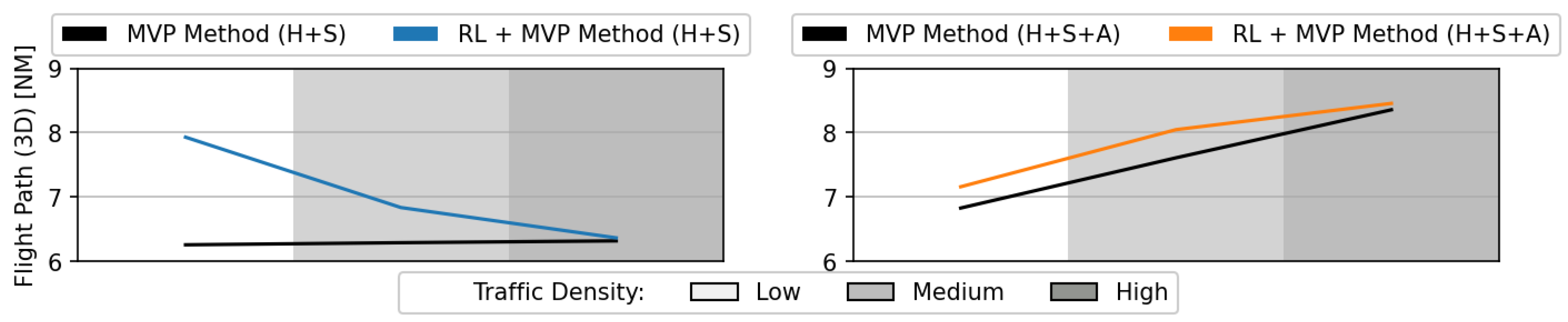
6.2.3. Efficiency Analysis
Figure 17 and
Figure 18 show the flight time and 3D flight path, per aircraft, during testing of the RL method, respectively. The total flight time was a direct result of the time in conflict (see
Figure 13). The resolution of the higher number of conflicts also increased the 3D path travelled as aircraft moved away from their nominal, straight path to resolve conflicts.
7. Discussion
Recent studies have focused on using RL approaches to decide the state deviation that aircraft should adopt for successful CR. However, the efficacy of these methods still cannot surpass the performance of state-of-the-art geometric CR algorithms at higher traffic densities. This study posed the question of whether the RL method could, instead, be used to improve the behaviour of these geometric CR algorithms. This was an exploratory work in which an RL method was used to generate the parameters used by an CR algorithm to generate a CR manoeuvre.
The results showed that a hybrid method, combining the strengths of both RL and geometric CR algorithms, led to fewer losses of minimum separation when compared to using fixed, predefined rules for CR. The benefit from the RL method lay on (1) the ability to determine how far in advance the ownship should initiate the CR manoeuvre and (2) in which directions to resolve the conflict. The former allowed for the prioritising of short-term conflicts or the advanced defence against far away conflicts. The latter induced an heterogeneity of the directions that aircraft used to move out of a conflict, which could be beneficial as it prevented aircraft from moving in the same direction. The following subsections further develop these topics.
Finally, questions remain regarding the application of this RL approach to other geometric CR methods and operational environments. Here, the RL method had a limited action formulation, being responsible for modelling only four parameters. Nevertheless, a generation of a conflict resolution manoeuvre can include a multitude of parameters. Additionally, the efficacy of a hybrid RL + CR method is dependent on the RL understanding how the values affect the performance of the CR algorithm. More research is needed to determine whether this approach can be successfully applied in a real-world scenario.
7.1. Conflict Prioritisation
By controlling look-ahead time, the RL method selected against which layers of aircraft the ownship would defend. With shorter look-ahead values, the ownship defended against the closest layers of aircraft, prioritising short-term conflicts. With larger look-ahead values, a higher number of layers of aircraft were defended against, and conflicts were resolved with more time in advance. However, considering a greater number of intruders in the generation of the resolution could make the final CR manoeuvre less effective against each of these intruders.
The RL method prioritised short-term conflicts when the surrounding aircraft were closer in time to a loss of minimum separation. This ensured that CR focussed only on these conflicts, increasing the likelihood of successfully resolving them. Larger look-ahead values were employed when the surrounding aircraft were farther away. In a way, the look-ahead values varied so that a limited number of aircraft were included in the generation of the CR manoeuvre.
Furthermore, how far the RL method defended in advance depended on the efficacy of the CR manoeuvre. With a less efficient manoeuvre, the RL method understood that a longer reaction time was needed, as the manoeuvre employed needed a longer time to establish a safe distance. On the contrary, when altitude variation was used to resolve conflicts, lower look-ahead values were used. As all aircraft flew at the same altitude, climbing or descending was a powerful tool, moving the ownship out of the main traffic layer. Thus, less reaction time was needed in that case.
7.2. Heterogeneity of Conflict Resolution Directions
The RL method found that, to resolve a conflict, moving the ownship in multiple directions simultaneously was beneficial. However, altitude or heading deviations were less effective when intruding aircraft moved in the same direction to resolve the conflict. The RL method understood that having different combinations of state variations (i.e., heading, speed, and/or altitude variation) led the intruding aircraft to resolve in different directions, increasing the chances of the resolution manoeuvres being effective.
It can be considered that the biggest advantage of allowing a CR algorithm to control multiple degrees of freedom is the ability to use different combinations of state variations to resolve conflicts. However, this heterogeneity should be based on rules to ensure that different combinations are used per aircraft in conflict with each other. From the results obtained, it was not clear how the RL method made these decisions.
7.3. Future Work
The values chosen by the RL method depended on the operational environment, flight routes, and performance limits of the aircraft involved. Future work will explore this RL approach under uncertainties. In this case, it is likely that smaller look-ahead times would be picked, as higher values would entail the propagation of more uncertainties. Additionally, having a single RL method responsible for separating aircraft under position uncertainties may lead the method to adopt a more defensive stance and start considering bigger separation distances. The latter will lead to larger CR manoeuvres, which, in turn, increase flight path and time. A better option may be to have a second RL method responsible for determining the most likely position of the intruders under uncertainties [
36]. This new position would then be used by the RL method responsible for guaranteeing the minimum separation between aircraft.
Finally, future work can benefit from using RL methods to directly prioritise specific intruders. This is far from a trivial task. Previous work has shown that a large amount of training is necessary for an RL method to understand the effect of enabling/disabling each intruder in the generation of a CR manoeuvre [
37]. However, it is of interest to explore this area of research. Different aircraft at similar look-ahead values can then be included/excluded from the CR manoeuvre.
8. Conclusions
This paper proposed a different application of reinforcement learning (RL) in the area of conflict resolution. RL is typically used as the method that is fully responsible for safeguarding the separation between aircraft. Although great progress has been made in this area, these methods cannot yet surpass the performance of the state-of-the-art distributed, geometric CR methods. This works used RL, instead, to help improve the efficacy of the latter geometric methods. This article employed an RL method responsible for optimising the values that a geometric CR algorithm used for the generation of conflict resolution manoeuvres. Namely, the RL was responsible for defining the look-ahead time at which the geometric CR method started defending against conflicts, as well as in which directions to move towards a nonconflicting trajectory.
The advantage of RL approaches is that they can find optimal solutions to a multitude of different conflict geometries, which would be arduous to develop through man-written rules. The hybrid combination of RL + CR successfully obtained fewer losses of minimum separation than a baseline CR method which used hard-coded, predefined values for all conflict geometries. The main benefits resulted from (1) the prioritisation of conflicts depending on the degrees of freedom and (2) the heterogeneity of deconflicting directions between aircraft in a conflict situation. These two rules improved the resolution of conflicts at different traffic densities.
However, more research is needed to validate whether this approach is still effective in real-world scenarios under uncertainties, which can increase the gap between the practical efficacy of RL methods and its expected theoretical performance. Additionally, future work will focus on translating this application to other geometric CR algorithms and operational environments. The work performed herein was focused solely on one geometric CR algorithm that took two values as input. To fully analyse whether RL approaches can define the best values for the generation of CR manoeuvres, this work must be expanded to different algorithms, especially those with a larger number of variables.


