
Analytic Solution of Optimal Aspect Ratio of Bionic Transverse V-Groove for Drag Reduction Based on Vorticity Kinetics
Abstract
:1. Introduction
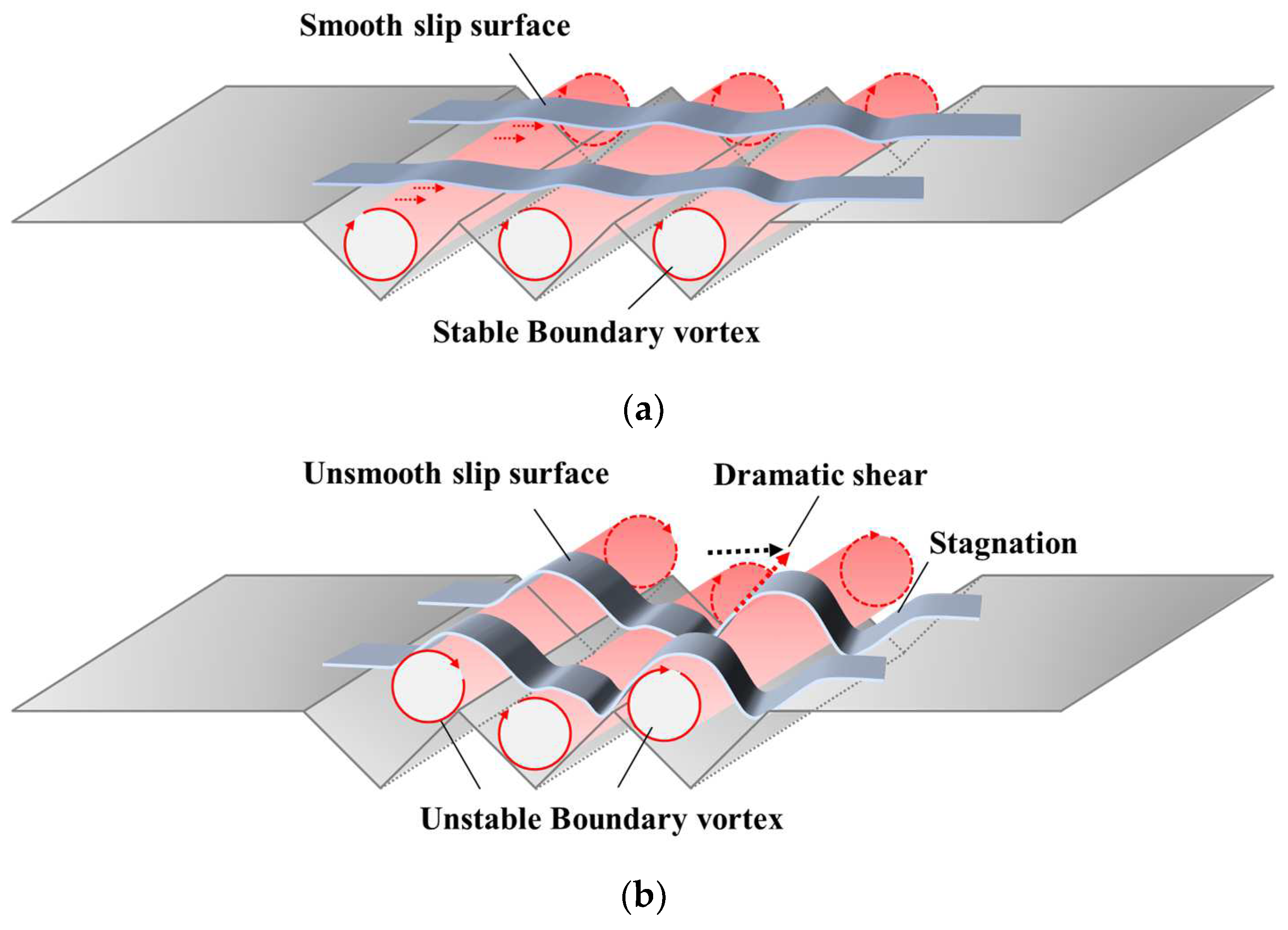
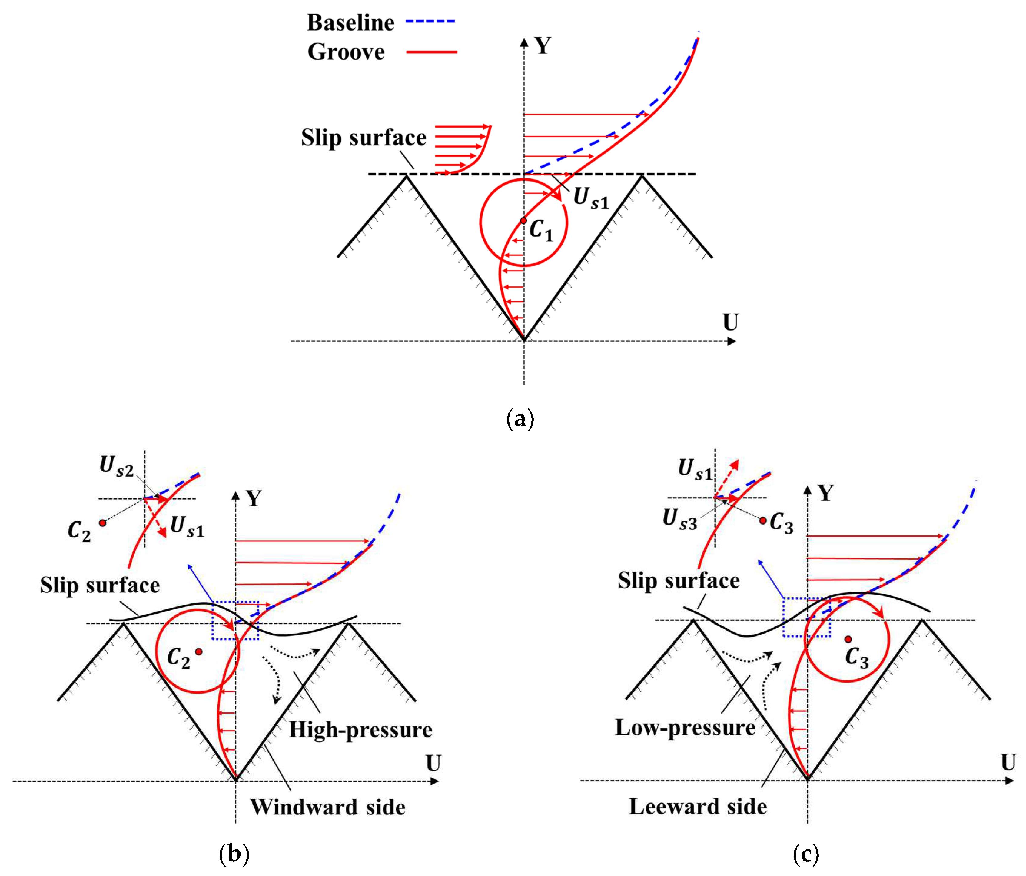
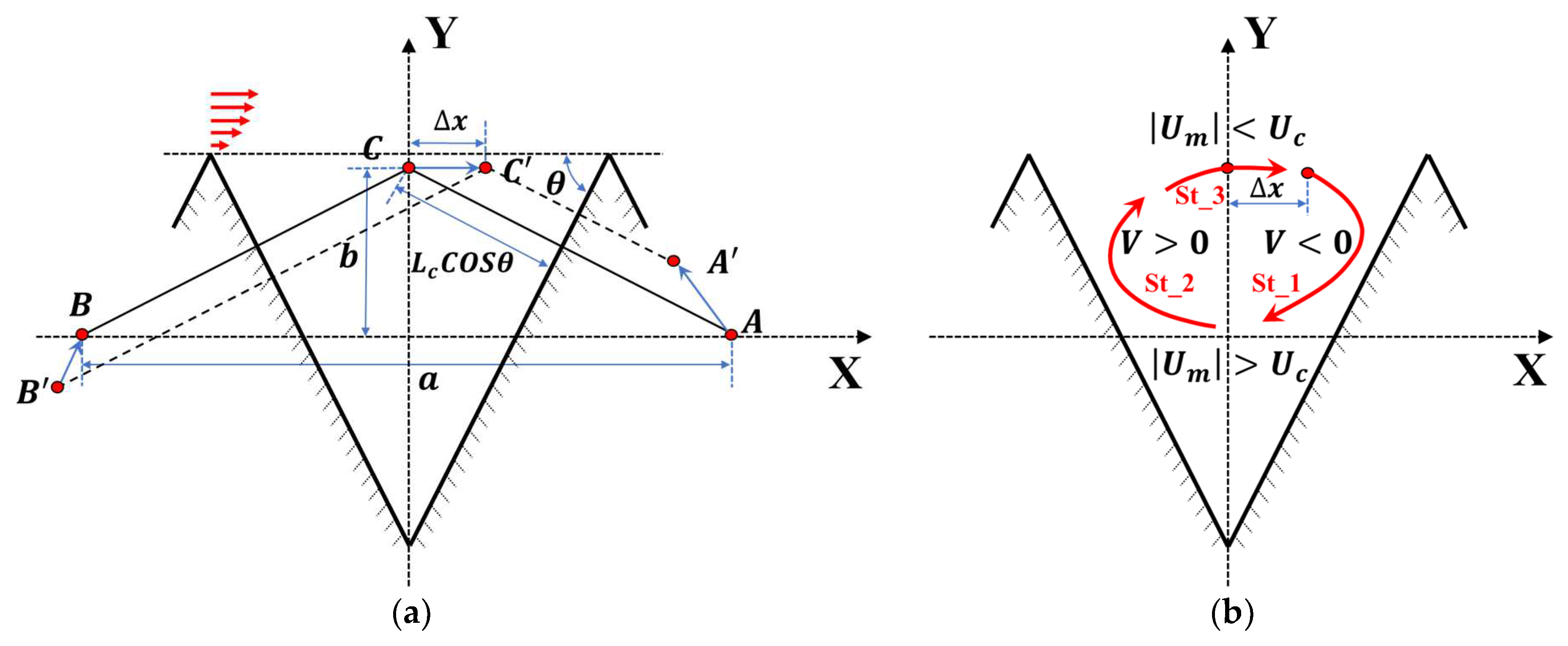
2. Influence of Boundary Vortex Stability on Drag-Reduction Performance
3. Theoretical Solution of AR for Maintaining the Stability of Boundary Vortices
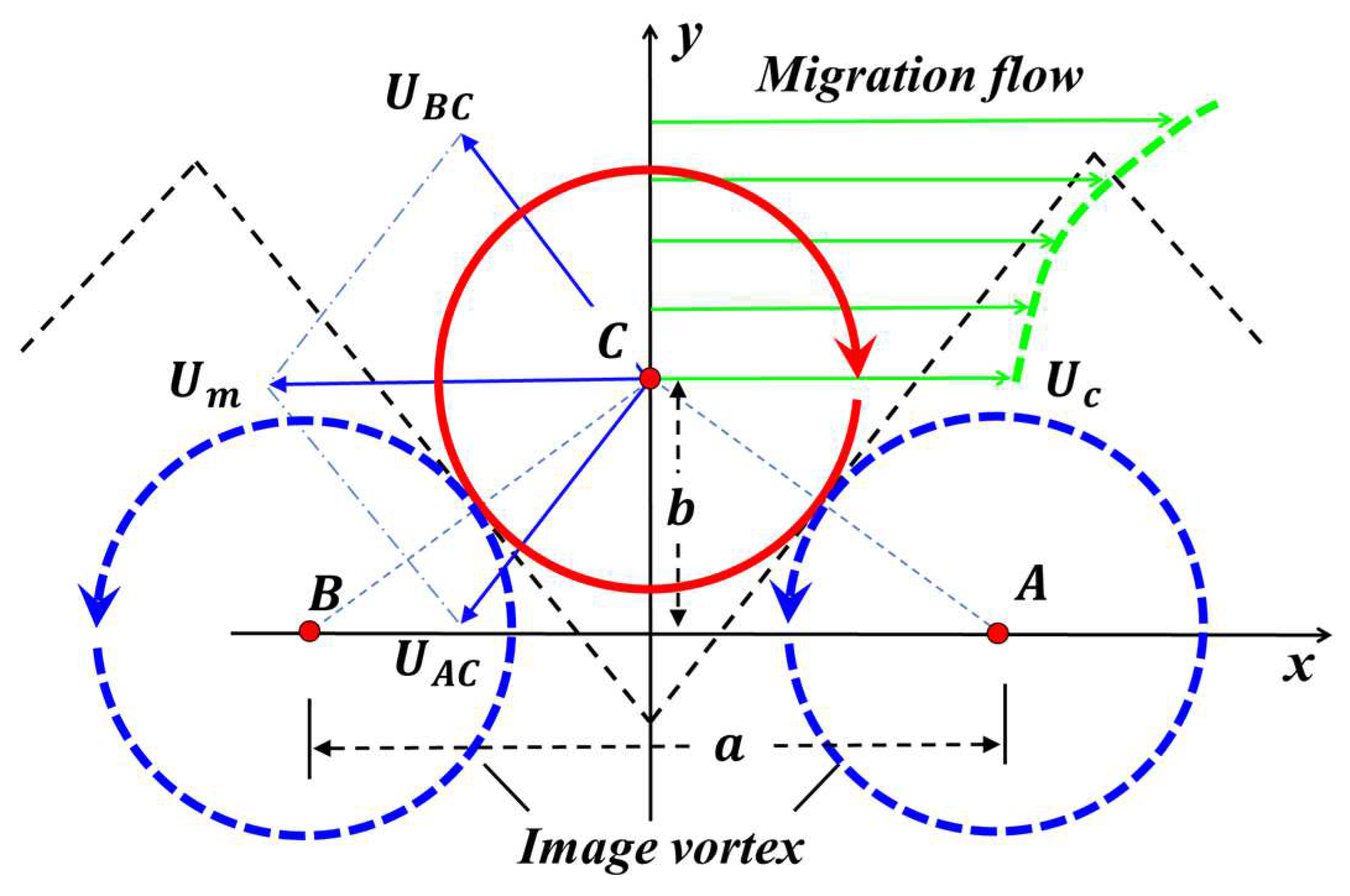
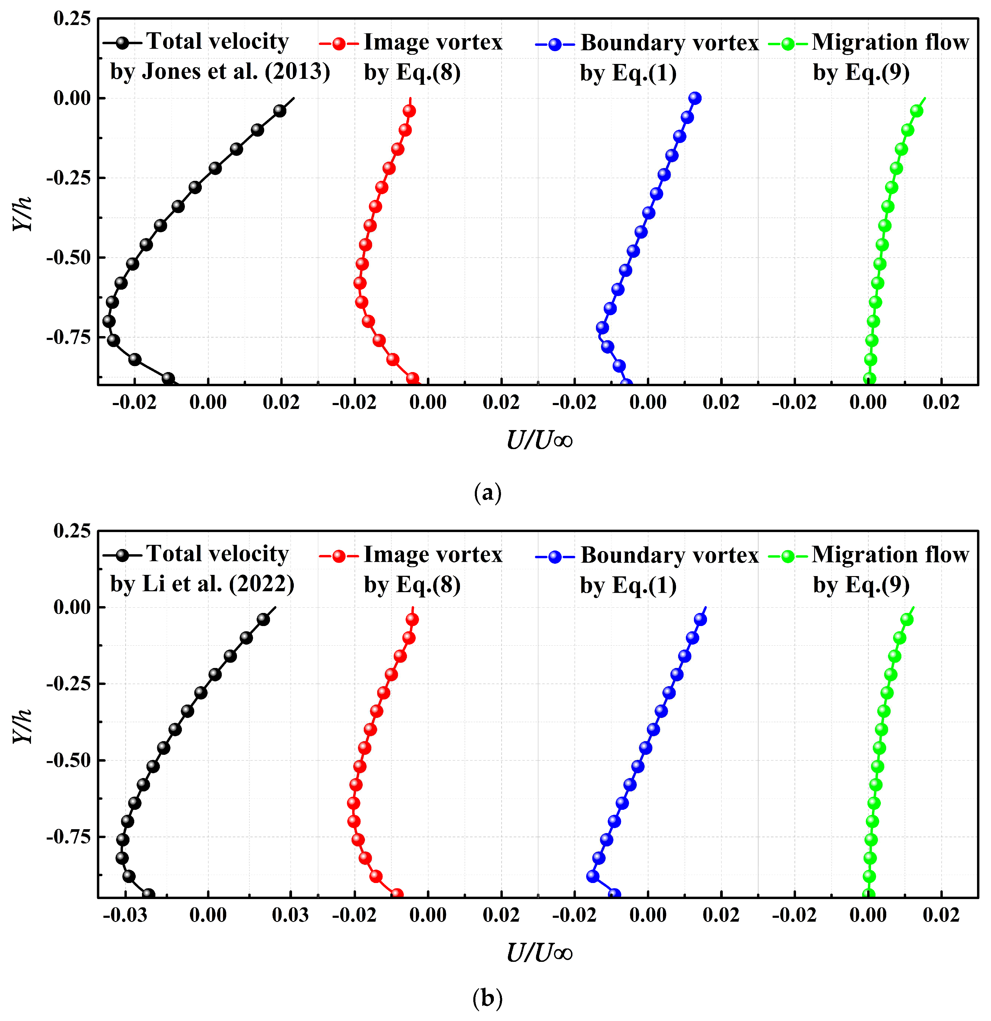
3.1. Induced Velocity Induced by Image Vortices
3.2. Migration Velocity Decomposed by Total Velocity
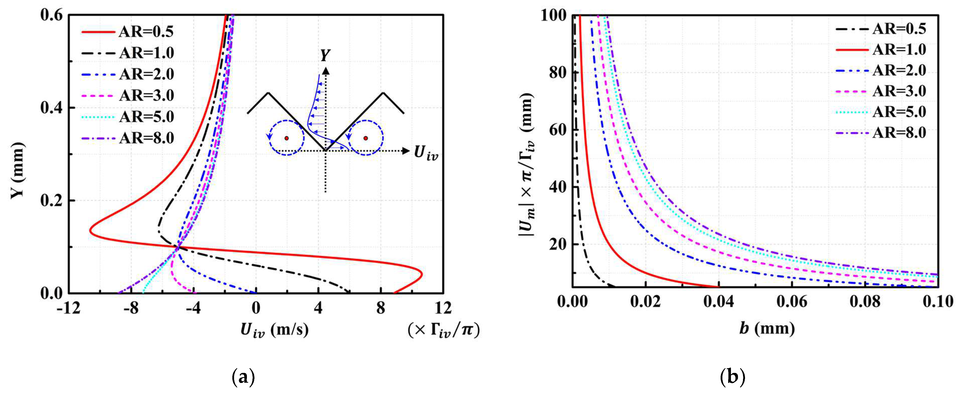
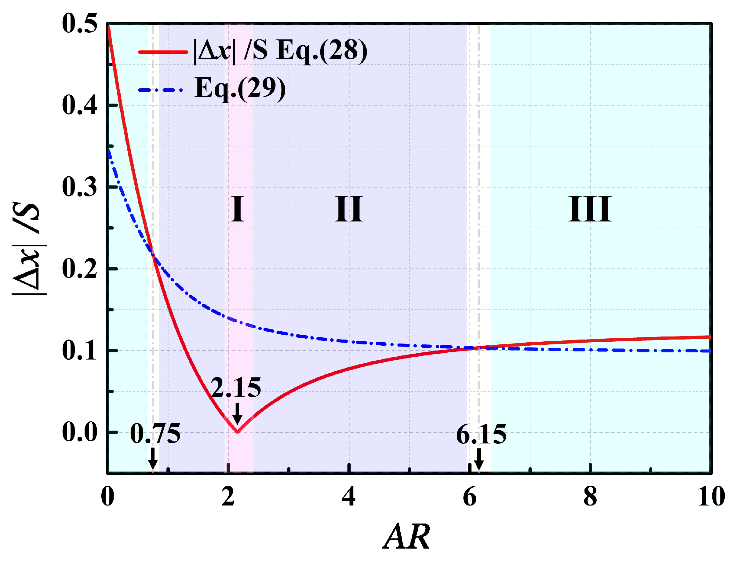
3.3. Solution of Aspect Ratio Based on Equalization between Induced Velocity and Migration Velocity
4. Numerical Verification
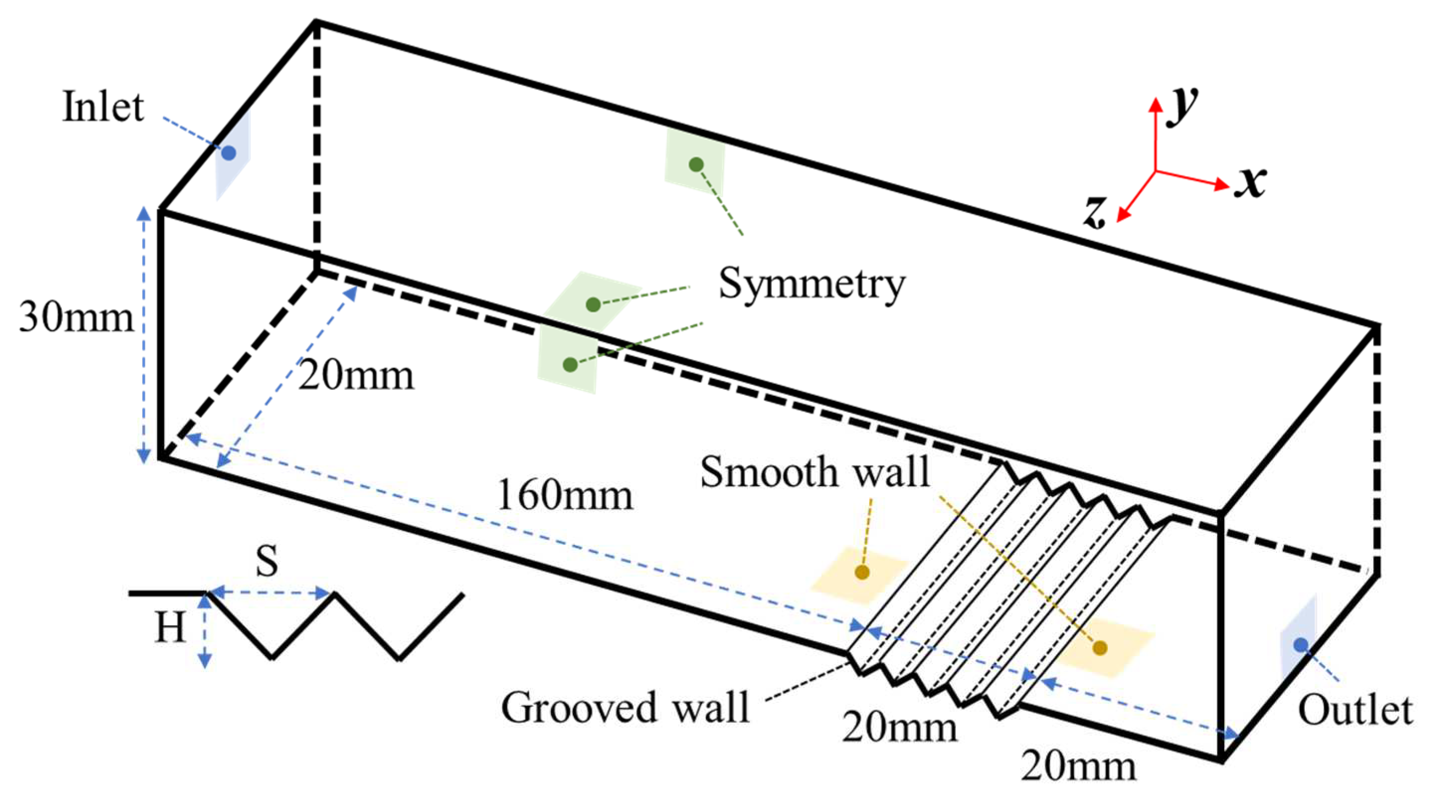
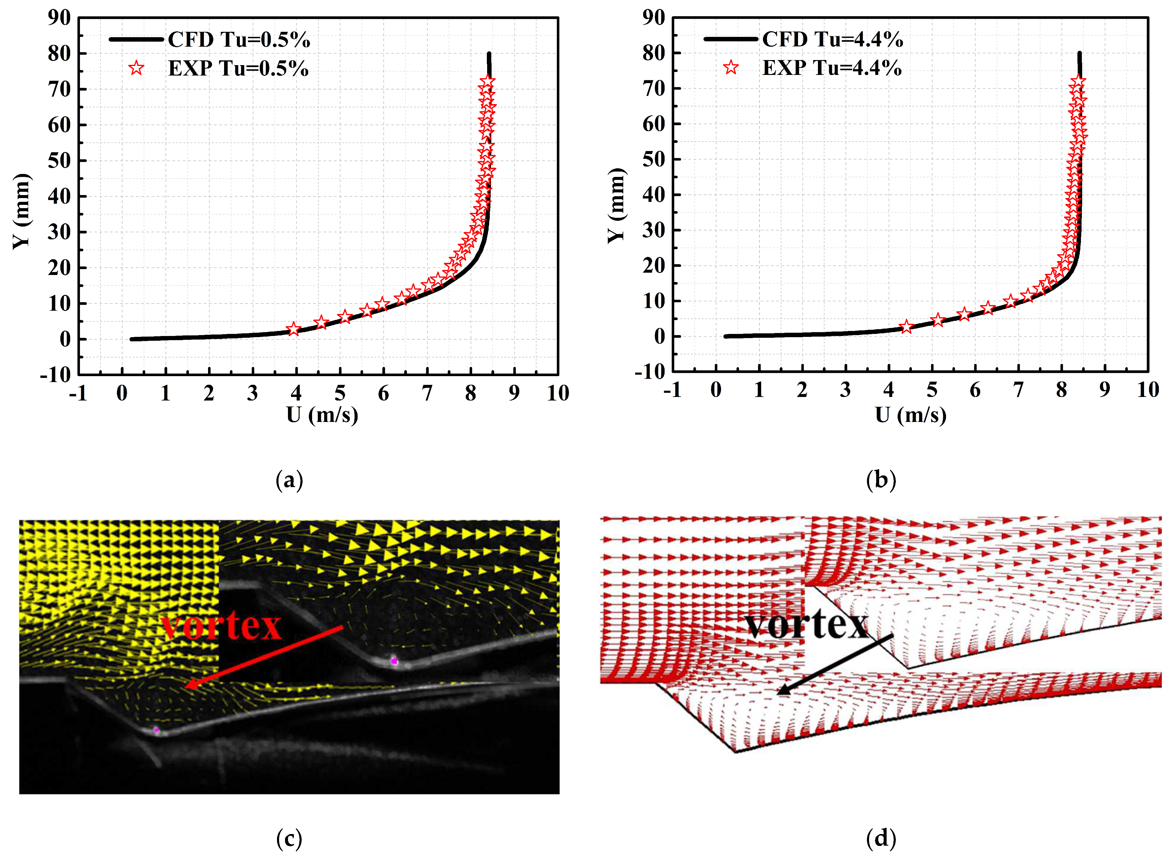
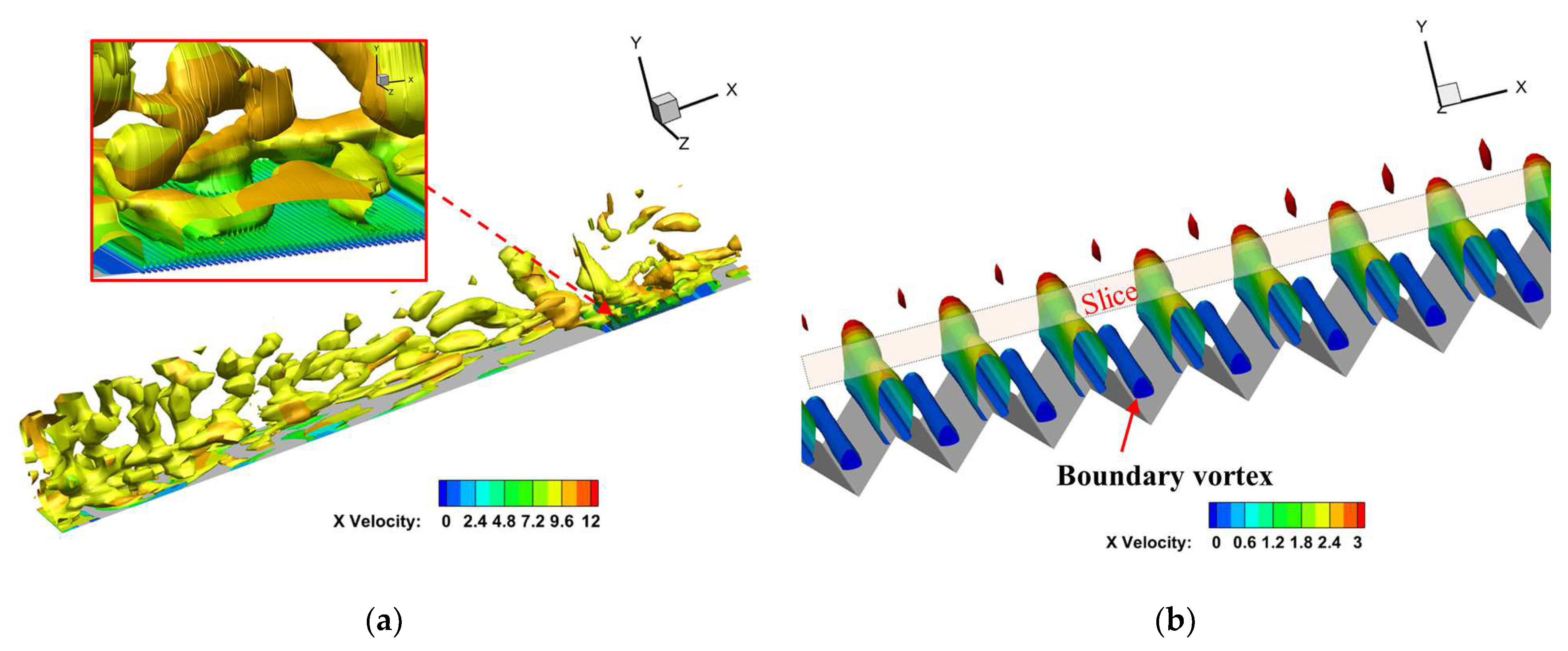
4.1. Numerical Methodology
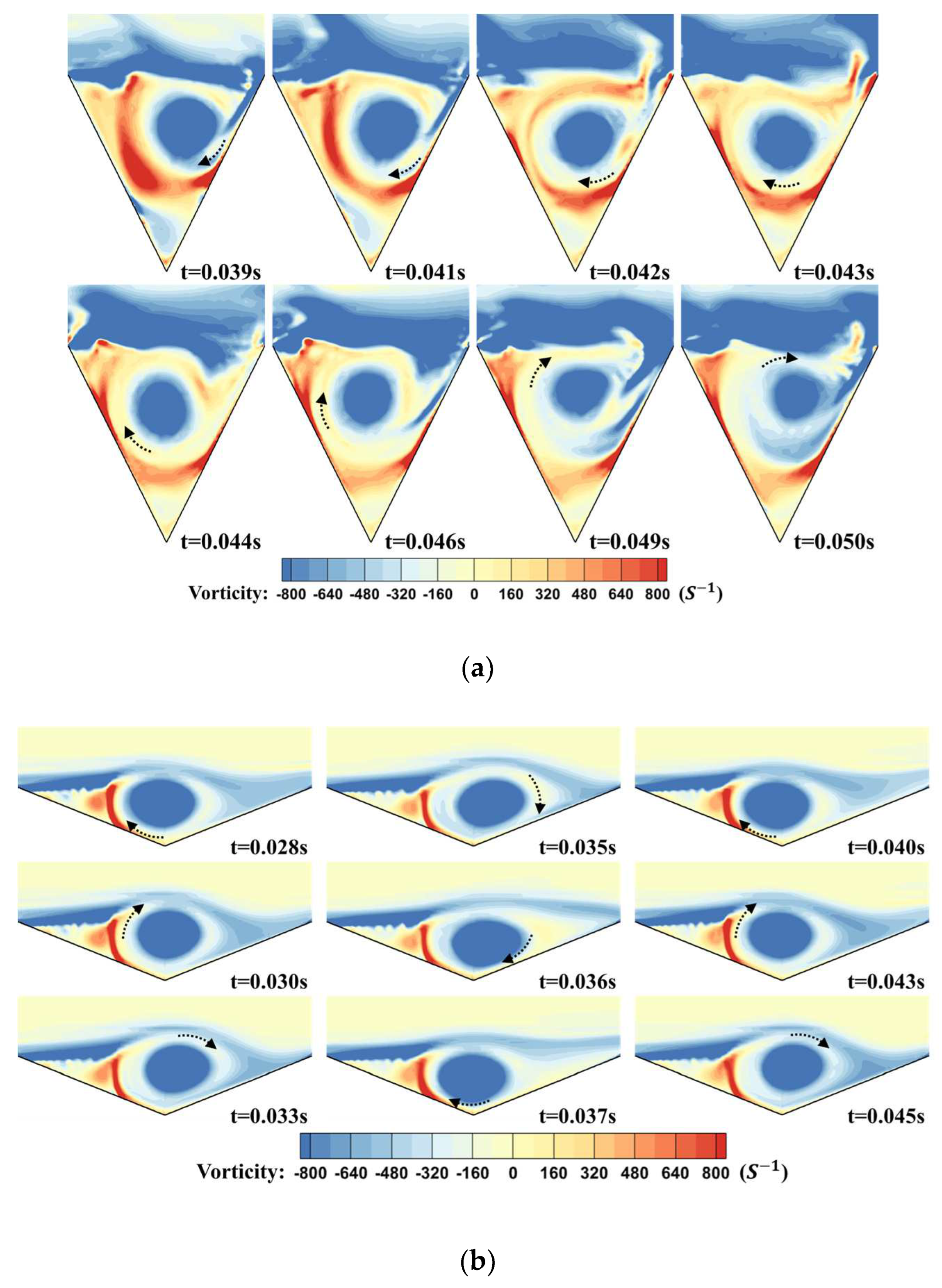
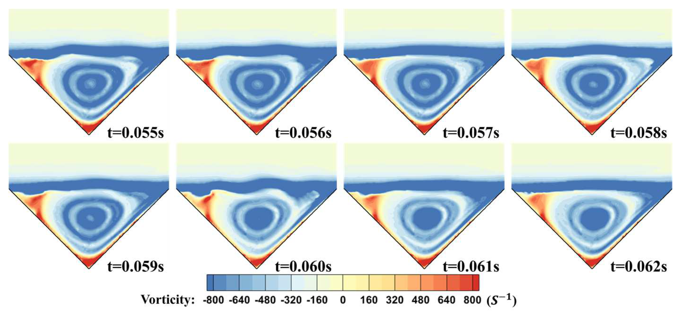
4.2. Stability of Boundary Vortices and Drag-Reduction Rate of Transverse Grooves with Different ARs
5. Conclusions
- (1)
- The velocity potential of the groove sidewalls to the boundary vortex is described by an image vortex model, thus establishing the relationship between the AR and the induced velocity. Secondly, the velocity profile of the migration flow is obtained by decomposing the total velocity inside the groove, by which the relationship between the AR and the migration velocity is established. Finally, the analytical solution of the optimal AR () is obtained based on the kinetic conditions (i.e., the induced velocity is equal to the migration velocity) of the boundary vortex stability and the value of the critical ARs ( and ) for which the boundary vortex can slosh inside the groove is obtained. Without considering the adverse pressure gradient and external disturbance, the motion forms of the boundary vortex inside the groove can be divided into three forms with the variation in the AR.
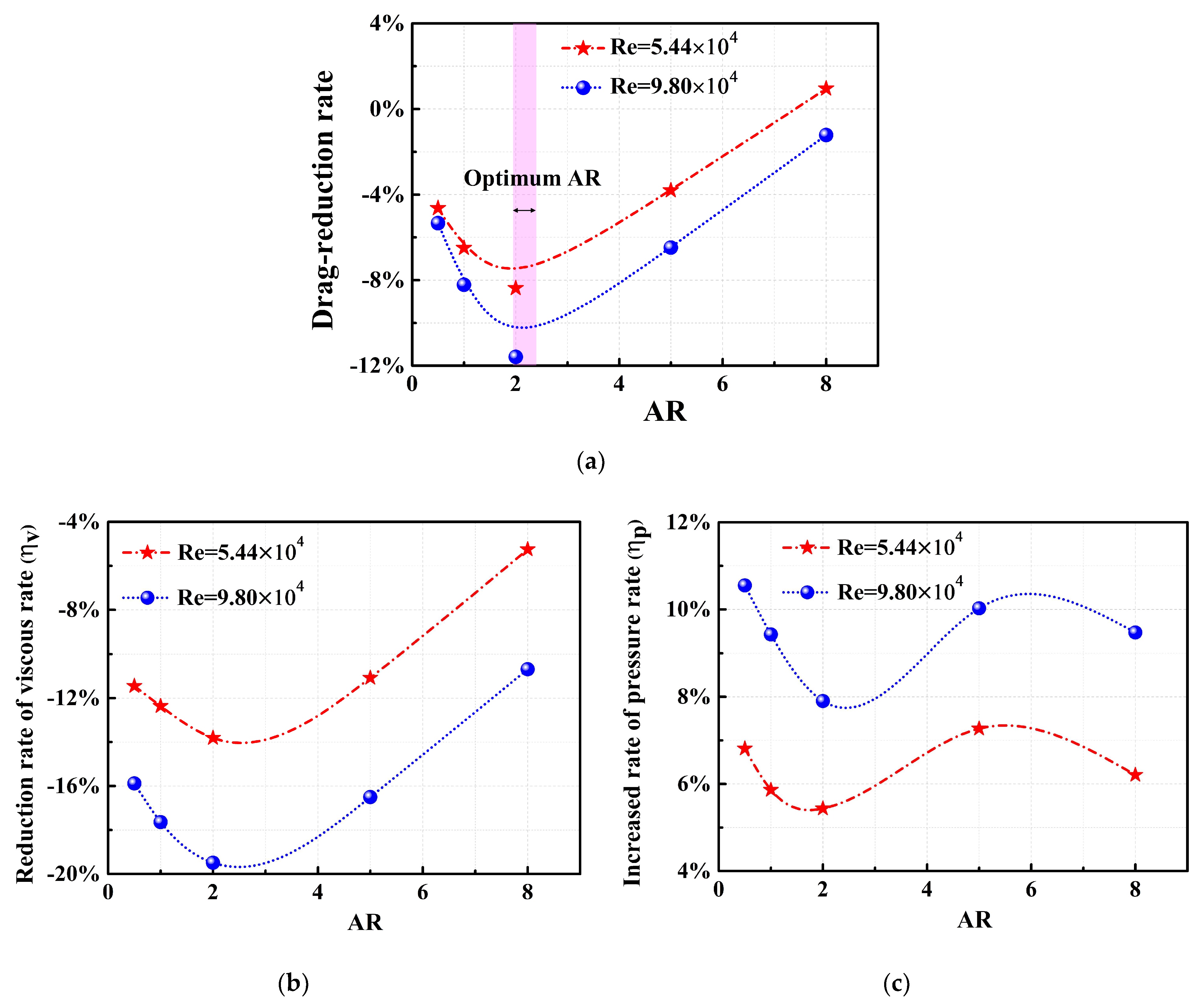
- (2)
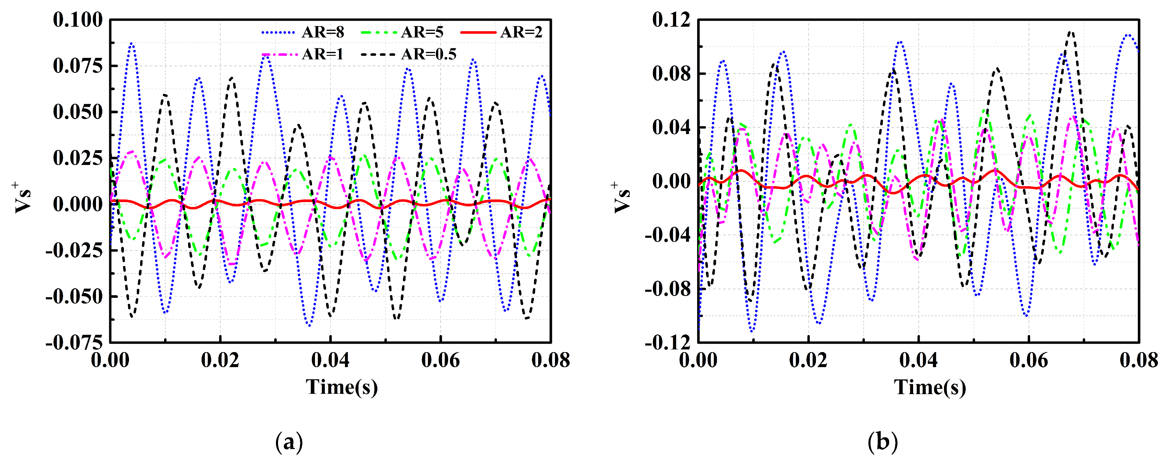
- The theoretical model for solving the optimal AR () and critical ARs ( and ) is validated by investigating the motion of the boundary vortices and the drag-reduction rate of the groove for ARs of 0.5, 1, 2, 5, and 8 with large eddy simulations. For AR = 2, the boundary vortex is stable inside the groove, corresponding to the maximum drag-reduction rate. When the AR is closer to 2, i.e., AR = 1 and AR = 5 (corresponds to the interval and ), the boundary vortices slosh periodically inside the groove and the magnitude of the vertical velocity fluctuations is similar in both cases. This periodic motion of the boundary vortex in the groove is classified as the “vortex sloshing” phenomenon. When the AR is far from 2, i.e., AR = 0.5 and AR = 8 (corresponds to the interval and ), the boundary vortices are shed from the shear layer at the leeward side and migrate downstream with the mainstream, which is classified as the “vortex shedding” phenomenon and corresponds to the minimum drag-reduction rate.
Author Contributions
Funding
Data Availability Statement
Conflicts of Interest
References
- Yu, J.C.; Wahls, R.A.; Esker, B.M.; Lahey, L.T.; Akiyama, D.G.; Drake, M.L.; Christensen, D.P. Total Technology Readiness Level: Accelerating Technology Readiness for Aircraft Design. In Proceedings of the AIAA Aviation 2021 Forum, Virtual Conference, 2–6 August 2021; p. 2454. [Google Scholar]
- Wainwright, D.K.; Fish, F.E.; Ingersoll, S.; Williams, T.M.; St Leger, J.; Smits, A.J.; Lauder, G.V. How smooth is a dolphin? The ridged skin of odontocetes. Biol. Lett. 2019, 15, 20190103. [Google Scholar] [CrossRef] [PubMed]
- Lang, A.W.; Jones, E.M.; Afroz, F. Separation control over a grooved surface inspired by dolphin skin. Bioinspiration Biomim. 2017, 12, 026005. [Google Scholar] [CrossRef] [PubMed]
- Li, Z.; He, L.; Zheng, Y. Quasi-Analytical Solution of Optimum and Maximum Depth of Transverse V-Groove for Drag Reduction at Different Reynolds Numbers. Symmetry 2022, 14, 342. [Google Scholar] [CrossRef]
- Wu, Z.; Li, S.; Liu, M.; Wang, S.; Yang, H.; Liang, X. Numerical research on the turbulent drag reduction mechanism of a transverse groove structure on an airfoil blade. Eng. Appl. Comput. Fluid Mech. 2019, 13, 1024–1035. [Google Scholar] [CrossRef] [Green Version]
- Wang, L.; Wang, C.; Wang, S.; Sun, G.; You, B.; Hu, Y. A novel ANN-Based boundary strategy for modeling micro/nanopatterns on airfoil with improved aerodynamic performances. Aerosp. Sci. Technol. 2022, 121, 107347. [Google Scholar] [CrossRef]
- Choi, K.S.; Fujisawa, N. Possibility of drag reduction usingd-type roughness. Appl. Sci. Res. 1993, 50, 315–324. [Google Scholar] [CrossRef]
- Lee, C.; Lee, G.W.; Choi, W.; Yoo, C.H.; Chun, B.; Lee, J.S.; Jung, H.W. Pattern flow dynamics over rectangular Sharklet patterned membrane surfaces. Appl. Surf. Sci. 2020, 514, 145961. [Google Scholar] [CrossRef]
- Tirandazi, P.; Hidrovo, C.H. Study of drag reduction using periodic spanwise grooves on incompressible viscous laminar flows. Phys. Rev. Fluids 2020, 5, 064102. [Google Scholar] [CrossRef]
- Chen, H.; Gao, Y.; Stone, H.A.; Li, J. “Fluid bearing” effect of enclosed liquids in grooves on drag reduction in microchannels. Phys. Rev. Fluids 2016, 1, 083904. [Google Scholar] [CrossRef]
- Davies, J.; Maynes, D.; Webb, B.W.; Woolford, B. Laminar flow in a microchannel with superhydrophobic walls exhibiting transverse ribs. Phys. Fluids 2006, 18, 087110. [Google Scholar] [CrossRef]
- Wang, B.; Wang, J.; Chen, D. A prediction of drag reduction by entrapped gases in hydrophobic transverse grooves. Sci. China Technol. Sci. 2013, 56, 2973–2978. [Google Scholar] [CrossRef]
- Wang, B.; Wang, J.; Zhou, G.; Chen, D. Drag reduction by microvortexes in transverse microgrooves. Adv. Mech. Eng. 2014, 6, 734012. [Google Scholar] [CrossRef]
- Wang, L.; Wang, C.; Wang, S.; Sun, G.; You, B. Design and analysis of micro-nano scale nested-grooved surface structure for drag reduction based on ‘Vortex-Driven Design’. Eur. J. Mech. B/Fluids 2021, 85, 335–350. [Google Scholar] [CrossRef]
- Wu, Z.; Yang, Y.; Liu, M.; Li, S. Analysis of the influence of transverse groove structure on the flow of a flat-plate surface based on Liutex parameters. Eng. Appl. Comput. Fluid Mech. 2021, 15, 1282–1297. [Google Scholar] [CrossRef]
- Mariotti, A.; Grozescu, A.N.; Buresti, G.; Salvetti, M.V. Separation control and efficiency improvement in a 2D diffuser by means of contoured cavities. Eur. J. Mech. B/Fluids 2013, 41, 138–149. [Google Scholar] [CrossRef]
- Mariotti, A.; Buresti, G.; Salvetti, M.V. Use of multiple local recirculations to increase the efficiency in diffusers. Eur. J. Mech. B/Fluids 2015, 50, 27–37. [Google Scholar] [CrossRef]
- Pasqualetto, E.; Lunghi, G.; Mariotti, A.; Salvetti, M.V. Spanwise-Discontinuous Grooves for Separation Delay and Drag Reduction of Bodies with Vortex Shedding. Fluids 2022, 7, 121. [Google Scholar] [CrossRef]
- Howard, F.; Goodman, W.; Walsh, M. Axisymmetric bluff-body drag reduction using circumferential grooves. In Proceedings of the Applied Aerodynamics Conference, Hampton, VA, USA, 13–15 July 1983; p. 1788. [Google Scholar]
- Lang, A.; Motta, P.; Habegger, M.L.; Hueter, R. Shark skin boundary layer control. In Natural Locomotion in Fluids and on Surfaces; Springer: New York, NY, USA, 2022; pp. 139–150. [Google Scholar]
- Cui, J.; Fu, Y. A numerical study on pressure drop in microchannel flow with different bionic micro-grooved surfaces. J. Bionic Eng. 2012, 9, 99–109. [Google Scholar] [CrossRef]
- Wu, L.; Jiao, Z.; Song, Y.; Liu, C.; Wang, H.; Yan, Y. Experimental investigations on drag-reduction characteristics of bionic surface with water-trapping microstructures of fish scales. Sci. Rep. 2018, 8, 12186. [Google Scholar] [CrossRef] [Green Version]
- Wu, L.; Jiao, Z.; Song, Y.; Ren, W.; Niu, S.; Han, Z. Water-trapping and drag-reduction effects of fish Ctenopharyngodon idellus scales and their simulations. Sci. China Technol. Sci. 2017, 60, 1111–1117. [Google Scholar] [CrossRef]
- Liu, W.; Ni, H.; Wang, P.; Zhou, Y. An investigation on the drag reduction performance of bioinspired pipeline surfaces with transverse microgrooves. Beilstein J. Nanotechnol. 2020, 11, 24–40. [Google Scholar] [CrossRef] [PubMed] [Green Version]
- Li, L.; Zhu, J.; Li, J.; Song, H.; Zeng, Z.; Wang, G.; Xue, Q. Effect of vortex frictional drag reduction on ordered microstructures. Surf. Topogr. Metrol. Prop. 2019, 7, 025008. [Google Scholar] [CrossRef]
- Bhatia, D.; Li, G.; Lin, Y.; Sun, J.; Barrington, P.; Li, H.; Wang, J. Transition delay and drag reduction using biomimetically inspired surface waves. J. Appl. Fluid Mech. 2020, 13, 1207–1222. [Google Scholar] [CrossRef]
- Liu, M.; Li, S.; Wu, Z.; Zhang, K.; Wang, S.; Liang, X. Entropy generation analysis for grooved structure plate flow. Eur. J. Mech. B/Fluids 2019, 77, 87–97. [Google Scholar] [CrossRef]
- Gautam, S. An Experimental Study of Drag Reduction Due to the Roller Bearing Effect over Grooved Surfaces Inspired by Butterfly Scales. Ph.D. Dissertation, The University of Alabama, Tuscaloosa, AL, USA, 2021. [Google Scholar]
- Tan, H.F.; Kang, J.T.; Wang, C.G. Study on grooved wall flow under rarefied condition using the lattice Boltzmann method. Int. J. Mech. Sci. 2015, 90, 1–5. [Google Scholar] [CrossRef]
- Milne-Thomson, L.M. Theoretical Hydrodynamics; Courier Corporation: Chelmsford, MA, USA, 1996. [Google Scholar]
- Greitzer, E.M.; Tan, C.S.; Graf, M.B. Internal Flow: Concepts and Applications; Cambridge University Press: Cambridge, UK, 2007. [Google Scholar]
- Doligalski, T.L.; Smith, C.R.; Walker, J.D.A. Vortex interactions with walls. Annu. Rev. Fluid Mech. 1994, 26, 573–616. [Google Scholar] [CrossRef]
- Ting, L.; Tung, C. Motion and decay of a vortex in a nonuniform stream. Phys. Fluids 1965, 8, 1039–1051. [Google Scholar] [CrossRef]
- Jones, E.M. An Experimental Study of Flow Separation Over a Flat Plate with 2D Transverse Grooves. Ph.D. Thesis, The University of Alabama, Tuscaloosa, AL, USA, 2013. [Google Scholar]
- Feng, B.; Chen, D.; Wang, J.; Yang, X. Bionic research on bird feather for drag reduction. Adv. Mech. Eng. 2015, 7, 849294. [Google Scholar] [CrossRef]
- Martin, S.; Bhushan, B. Fluid flow analysis of a shark-inspired microstructure. J. Fluid Mech. 2014, 756, 5–29. [Google Scholar] [CrossRef]
- Jiménez, J.; Moin, P. The minimal flow unit in near-wall turbulence. J. Fluid Mech. 1991, 225, 213–240. [Google Scholar] [CrossRef]
- Christophe, J.; Anthoine, J.; Moreau, S. Trailing edge noise of a controlled-diffusion airfoil at moderate and high angle of attack. In Proceedings of the 15th AIAA/CEAS Aeroacoustics Conference (30th AIAA Aeroacoustics Conference), Miami, FL, USA, 11–13 May 2009; p. 3196. [Google Scholar]
- Kraichnan, R.H. Diffusion by a random velocity field. Phys. Fluids 1970, 13, 22–31. [Google Scholar] [CrossRef]
- Smirnov, A.; Shi, S.; Celik, I. Random flow generation technique for large eddy simulations and particle-dynamics modeling. J. Fluids Eng. 2001, 123, 359–371. [Google Scholar] [CrossRef]
- Ahmadi-Baloutaki, M.; Carriveau, R.; Ting, D.K. Effect of free-stream turbulence on flow characteristics over a transversely-grooved surface. Exp. Therm. Fluid Sci. 2013, 51, 56–70. [Google Scholar] [CrossRef]
- Song, X.W.; Zhang, M.X.; Lin, P.Z. Skin friction reduction characteristics of nonsmooth surfaces inspired by the shapes of barchan dunes. Math. Probl. Eng. 2017, 2017, 6212605. [Google Scholar] [CrossRef]


| Dimensionless Parameters | Nodes | ||
|---|---|---|---|
| 2490 + 311 + 311 | 300 + 1000 + 60 | ||
| 466 | 80 | ||
| 311 | 80 | ||
| Groove | 0.3 | 1000 | |
| Other | <10 | 300 + 60 | |
| 0.02~10 | 80 | ||
| 3.9 | 80 | ||
| Drag (N) | Streamline | ||
|---|---|---|---|
| 0.3 | 3.9 | 0.00314 |  |
| 5.2 | 0.00313 | ||
| 1.2 | 3.9 | 0.00314 |  |
| 5.2 | 0.00315 |
| Variables | Value |
|---|---|
| (coarse) | 2,404,420 |
| (medium) | 4,123,710 |
| (fine) | 8,703,310 |
| 1.19 | |
| 1.28 | |
| p | 5.77 |
| 0.0860% | |
| 0.0159% | |
| 0.0795% | |
| 0.026% |
Publisher’s Note: MDPI stays neutral with regard to jurisdictional claims in published maps and institutional affiliations. |
© 2022 by the authors. Licensee MDPI, Basel, Switzerland. This article is an open access article distributed under the terms and conditions of the Creative Commons Attribution (CC BY) license (https://creativecommons.org/licenses/by/4.0/).
Share and Cite
Li, Z.; He, L.; Zuo, Y.; Meng, B. Analytic Solution of Optimal Aspect Ratio of Bionic Transverse V-Groove for Drag Reduction Based on Vorticity Kinetics. Aerospace 2022, 9, 749. https://doi.org/10.3390/aerospace9120749
Li Z, He L, Zuo Y, Meng B. Analytic Solution of Optimal Aspect Ratio of Bionic Transverse V-Groove for Drag Reduction Based on Vorticity Kinetics. Aerospace. 2022; 9(12):749. https://doi.org/10.3390/aerospace9120749
Chicago/Turabian StyleLi, Zhiping, Long He, Yueren Zuo, and Bo Meng. 2022. "Analytic Solution of Optimal Aspect Ratio of Bionic Transverse V-Groove for Drag Reduction Based on Vorticity Kinetics" Aerospace 9, no. 12: 749. https://doi.org/10.3390/aerospace9120749