Flight Procedure Analysis for a Combined Environmental Impact Reduction: An Optimal Trade-Off Strategy

Abstract

Many attempts have been made to reduce aviation’s environmental impact, as aviation traffic has grown exponentially in recent decades. While some approaches focus on technology and fuel alternatives, others strive to develop improved operational measures within air traffic management as a short-term action to mitigate aviation-induced climate change, as well as air pollution. In this work, different flight procedures are analyzed in terms of emissions and noise impact to define optimal trade-offs. The investigation is based on flight data recorders, emissions, and noise prediction models. An aircraft trajectory simulation code with flight procedure optimization is also implemented to define an environmentally optimal trajectory. The results show that while noise and the emissions proportional to the burned fuel may be reduced for some trajectories, other non-${\mathrm{CO}}_2$ emissions could drastically increase if too low idle-thrust levels are reached. Therefore, a minimum threshold for idle thrust is suggested as a key factor to define a truly optimal trajectory in terms of ${\mathrm{CO}}_2$ emissions, non-${\mathrm{CO}}_2$ emissions, and noise.

1. Introduction

The environmental impact of air transportation is of great concern due to the growing global demand for passenger mobility, affecting the climate, human health, and living conditions, especially around airports and surrounding communities. The European Environmental Agency and the European Parliament attribute air and noise pollution as being two of the major causes of cardiovascular and respiratory disease. Therefore, for the last decades, the problem of aircraft noise has been the main drive in the research area of environmental emissions [1,2,3]. However, whereas aircraft noise is limited to the airport’s surrounding area and disappears as the aircraft moves away, emission of combustion gasses, such as carbon dioxide (${\mathrm{CO}}_2$), nitrogen oxides (${\mathrm{NO}}_{\mathrm{x}}$), etc., is a permanent trace of air transportation. Aviation emissions, which account for more than 2% of global emissions and 13.4% of the emissions from transport, have already experienced a significant increase since 2005 by about 70%, and could reach over 300% by 2050 if no additional actions are taken [4,5]. Moreover, the total impact of aircraft emissions could be two up to four times larger than the impact of only ${\mathrm{CO}}_2$ [6,7], and aviation emissions have been shown to have a larger impact on air quality than on climate [8].

Different areas of focus within the aviation industry have seriously been taken into consideration in order to tackle these issues, supported as well by the Paris Agreement’s temperature goal, aiming to reduce global greenhouse gas emissions by at least 50% by 2050 compared to 1990 [9]. The four main environmental strategy areas are technical, fuel alternatives, operational, and regulations. This work belongs to the area of operational measures within air traffic management (ATM).

Extensive investigation has been carried out on the optimization of approach flight procedures and trajectories to reduce noise and, or gas emissions. Originally, the main drive was to minimize operational costs, heavily driven by fuel consumption. As ${\mathrm{CO}}_2$ emissions are directly linked to burned fuel, later on, this practice was claimed to be environmentally friendly, resulting in a win-win strategy for stakeholders and institutions [10,11,12]. Nevertheless, as previously mentioned, non-${\mathrm{CO}}_2$ emissions are known to have a relevant contribution to aviation-induced climate and air quality impacts, and must therefore be considered [13,14,15]. Moreover, by focusing only on ${\mathrm{CO}}_2$ emissions, the new apparently optimized trajectories could result in greater collateral damage in terms of noise, as well as non-${\mathrm{CO}}_2$ emissions not proportional to the total burned fuel, but dependent on the Mach number, fuel flow, and altitude or atmospheric conditions, such as carbon monoxide (CO), hydrocarbons (HC), and ${\mathrm{NO}}_{\mathrm{x}}$. Optimal flight procedures have already been defined for noise reduction [16], such as noise abatement departure procedure 1 (NADP 1) and NADP 2 [17], and steep-descent maneuvering for continuous descent approach (CDA) [18]. These procedures have resulted in some improvements in fuel or ${\mathrm{CO}}_2$ reduction. However, none of them consider the whole combined set of environmental variables in terms of all the main gas emissions from aircraft engines (${\mathrm{CO}}_2$ and non-${\mathrm{CO}}_2$) and noise, nor the impact of low idle-thrust levels below 7% engine power on HC and CO emissions. In fact, these emissions could dramatically increase due to their high sensitivity to the idling range [19]. For taxi and idling activities, it has been shown that with a 5% power setting, HC and CO emissions would increase by 132% and 58%, respectively [19].

This project aims to reduce noise and ${\mathrm{CO}}_2$ and non-${\mathrm{CO}}_2$ emissions through approach procedure analysis aiming to define optimal strategies, with a particular focus on CO, HC, and ${\mathrm{NO}}_{\mathrm{x}}$, which are especially associated with air quality and, therefore, public health. More specifically, the study considers ${\mathrm{CO}}_2$, CO, HC, ${\mathrm{NO}}_{\mathrm{x}}$, sulfur oxides (${\mathrm{SO}}_{\mathrm{x}}$), and water vapor (${\mathrm{H}}_2\mathrm{O}$) emissions, as well as noise. The Boeing Fuel Flow Method 2 [20] is used for the emissions modeling, which relies on the International Civil Aviation Organization (ICAO) emissions databank [21] and is complemented with the Aircraft Particle Emissions eXperiment (APEX) [22] study. Noise computation is carried out with the simulation of atmosphere and air traffic for a quieter environment (SAFT) code [3] using the European Civil Aviation Conference (ECAC) Doc 29 method. The flight procedures investigated correspond to real aircraft trajectories of a Boeing 737-800 based on flight data recorder (FDR) data. Two codes for trajectory simulation and flight procedure optimization have also been implemented for further analysis of the flight procedures.

The paper starts with a description of the models and data used for emissions and noise prediction, trajectory simulation, and flight procedure optimization. Afterward, different flight trajectories are analyzed in terms of their environmental impact, and an optimal trade-off strategy for flight procedures is identified and discussed.

2. Materials and Methods

This study is mainly based on FDR data provided by Scandinavian Airlines System (SAS), with which emissions and noise have been computed; the corresponding flight trajectories have been simulated for further analysis and optimization. Note that the International Standard Atmosphere (ISA) model has been used to compute the temperature and pressure at a given altitude for all the simulations.

2.1. Aircraft Model

The flight trajectories under consideration were simulated with a Boeing 737-800, the main characteristics of which are given in

Table 1. Characteristics of the Boeing 737-800.

Dimensions
Length	39.5 m
Wing span	34.3 m
Wing reference area (S)	124.6 m${}^2$
Max take-off weight (MTOW)	79,000 kg
Max fuel load	26,000 L
Passengers	max. 189
Engine performance (CFM56-7B27)
Max thrust	121.4 kN/engine
Fuel flow at cruise (typical)	2450 kg/h
Performance
Max cruise speed	Mach 0.82
Max cruise altitude	41,000 feet (FL41)

. The Boeing 737 is a turbofan jet aircraft developed in several configurations, whose first flight with the first version, the 737-100, took place in 1967. Since then, the aircraft has been upgraded continuously.

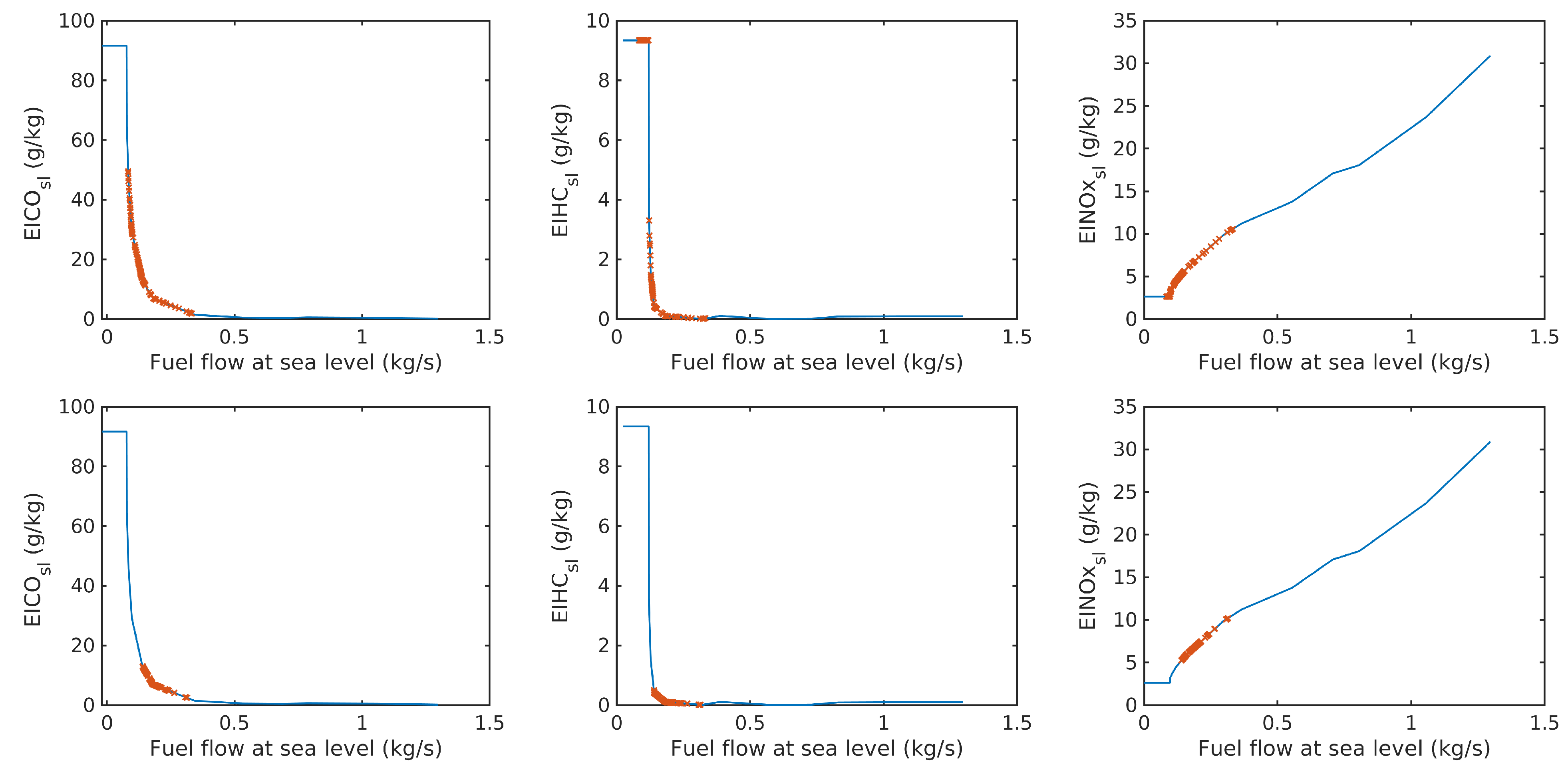
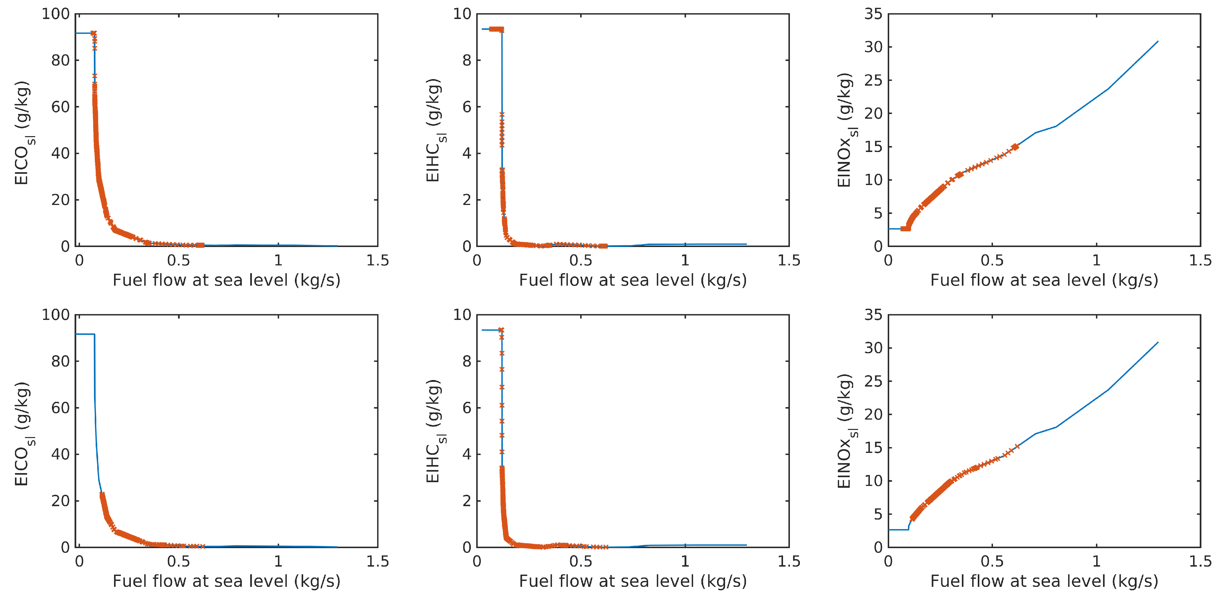
2.2. Emissions Model

The engine exhaust emissions considered in this study are ${\mathrm{CO}}_2$, $\mathrm{CO}$, $\mathrm{HC}$, ${\mathrm{NO}}_{\mathrm{x}}$, ${\mathrm{SO}}_{\mathrm{x}}$, and ${\mathrm{H}}_2\mathrm{O}$. The emissions modeling is based on the emissions indices (EIs), which correspond to the emissions in grams per kilogram of fuel consumed. Depending on the type of emission, a more or less complex model may be required. In the case of ${\mathrm{CO}}_2$, ${\mathrm{H}}_2\mathrm{O}$, and ${\mathrm{SO}}_{\mathrm{x}}$ emissions, they are modeled based only on jet fuel composition and are therefore proportional to the burned fuel through constant emissions indices [23].

$$\begin{array}{cc}\hfill EIC{O}_2& \hfill =3155\mathrm{g}/\left(\mathrm{kg}\mathrm{fuel}\right)\hfill \end{array}$$

(1)

$$\begin{array}{cc}\hfill EI{H}_{2}O& \hfill =1237\mathrm{g}/\left(\mathrm{kg}\mathrm{fuel}\right)\hfill \end{array}$$

(2)

$$\begin{array}{cc}\hfill EIS{O}_x& \hfill =0.8\mathrm{g}/\left(\mathrm{kg}\mathrm{fuel}\right)\hfill \end{array}$$

(3)

On the other hand, the computation of the remaining emissions indices requires a more complex model, and in this study, the Boeing Fuel Flow Method 2 [20] is used. The process of this method is illustrated in Figure 1.

The model relies on readily available data such as the engine fuel flow, obtained here through simulation, or FDR data at altitude level, $f_{\mathrm{alt}}$, read at each time step in the flight trajectory. The fuel-flow level at a given time is then corrected to a corresponding fuel flow at sea level, $f_{\mathrm{sl}}$; see Figure 1 step (1), Equation (7). The next step (2) requires a model of the sea level emissions indices as a function of fuel flow at sea level, namely $EIC{O}_{\mathrm{sl}}$, $EIH{C}_{\mathrm{sl}}$, and $EIN{O}_{x_{\mathrm{sl}}}$ (Section 2.2.1), giving the corresponding emission index value at sea level for the corrected fuel-flow level. Afterward, the emission index is corrected for altitude; see step (3), Equations (4)–(6).

$$\begin{array}{cc}\hfill EIC{O}_{\mathrm{alt}}& \hfill =EIC{O}_{\mathrm{sl}}\left(f_{\mathrm{sl}}\right)\frac{{\theta }^{3.3}}{{\delta }^{1.02}}\hfill \end{array}$$

(4)

$$\begin{array}{cc}\hfill EIH{C}_{\mathrm{alt}}& \hfill =EIH{C}_{\mathrm{sl}}\left(f_{\mathrm{sl}}\right)\frac{{\theta }^{3.3}}{{\delta }^{1.02}}\hfill \end{array}$$

(5)

$$\begin{array}{cc}\hfill EIN{O}_{x_{\mathrm{alt}}}& \hfill =EIN{O}_{x_{\mathrm{sl}}}\left(f_{\mathrm{sl}}\right)\sqrt{\frac{{\delta }^{1.02}}{{\theta }^{3.3}}}{e}^H\hfill \end{array}$$

(6)

with

$$f_{\mathrm{sl}}=f_{\mathrm{alt}}\frac{{\theta }^{3.8}}{\delta }{e}^{0.2M^2}$$

(7)

where M is the Mach number, $\theta =T/T_0$, and $\delta =P/P_0$. T is the temperature in Kelvin, P the pressure in Pa, and the corresponding constants at sea level are $T_0$ = 288.15 K and $P_0$ = 101,325 Pa. Moreover, H is a humidity correction factor [20], which has been computed according to [24].

Since emissions indices are computed at each time step and in grams per kilogram of fuel consumed, the actual total emissions in kilograms for a given flight trajectory still needs to be computed as in Equation (8) for each of the emissions.

$$HC=\frac{1}{1000}{\int }_0^{t_e}\left(EIH{C}_{\mathrm{alt}}{f}_{\mathrm{alt}}\right)\mathrm{d}t$$

(8)

This model considers for the emissions computation, the altitude, Mach number, fuel flow, and atmospheric conditions. The Boeing Fuel Flow Method 2 has already been successfully used in a previous investigation [25].

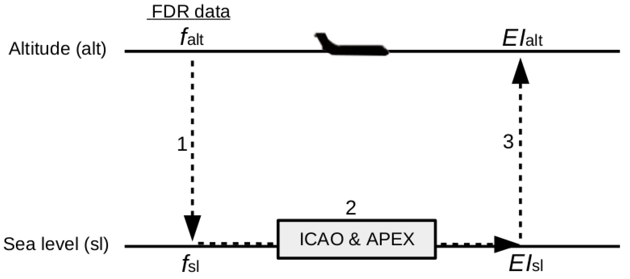
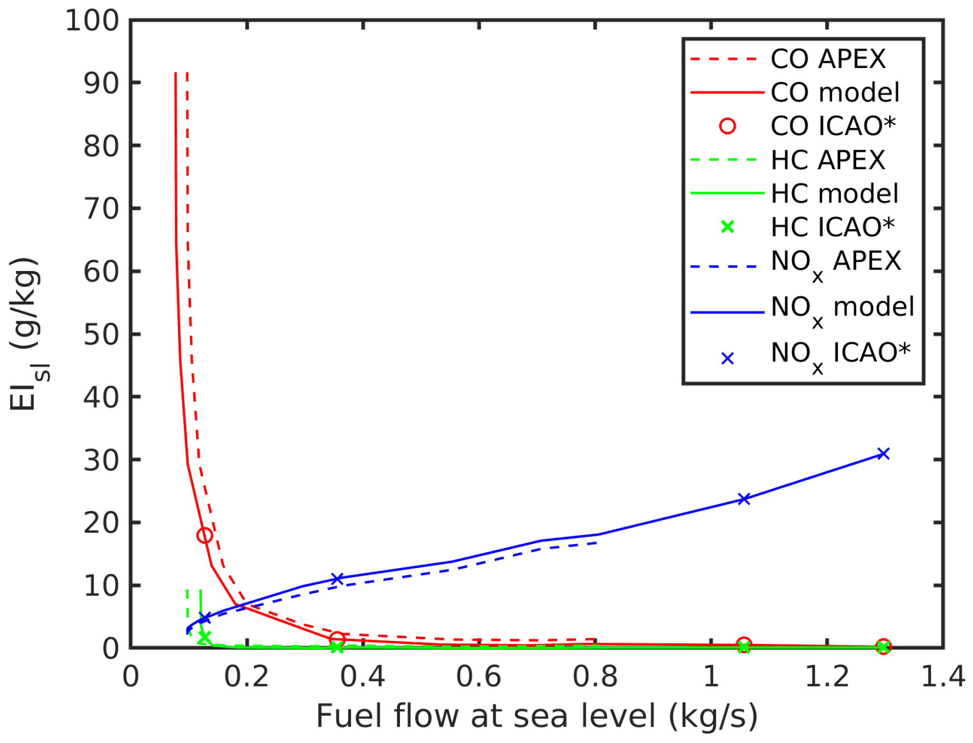
2.2.1. Method for Emission Index Modeling

The method for modeling the emission index at sea level (${\mathrm{EI}}_{\mathrm{sl}}$) with respect to fuel flow at sea level is based on the four certification data points from the ICAO emissions databank [21] for the engine type under consideration, here the CFM56-7B27, Table 1. These emissions data points are measured at sea level at different thrust levels correlated to different fuel-flow levels. Since the four data points do not cover the whole range of fuel-flow levels, particularly at idle thrust, the emissions data have been completed with the APEX [22] measurements performed for a similar engine, a General Electric CFM56-2-C1 engine. A minimum cap of 7% power setting is usually used to model emissions for idle thrust, such as in the Emissions and Dispersion Modeling System (EDMS) [26] and the Aviation Environmental Design Tool (AEDT) [27] to prevent erroneous predictions due to the lack of information; here, the APEX data is used to cover the commonly unknown and neglected critical area below 7%. Thereby, we aim to be more realistic, decreasing the resulting error and considering the worst case scenario [19]. This way, HC and CO will not be underpredicted and ${\mathrm{NO}}_{\mathrm{x}}$ will not be overpredicted.

The emission index models for CO, HC, and ${\mathrm{NO}}_{\mathrm{x}}$ are presented in Figure 2. They follow the same trends as the corresponding APEX data for each of the emissions while passing through the four certification data points from the ICAO emissions databank. Note that the corresponding fuel-flow values of the ICAO data points have been adjusted for installation effects by applying correction factors used in the Boeing Fuel Flow Method 2 [20]. From these curves and ICAO data points, strong discrepancies in terms of maximum ${\mathrm{EI}}_{\mathrm{sl}}$ levels for minimum idle thrust can be clearly observed, where ICAO data would result in a maximum cap level of 1.7 and 17.9 for HC and CO, respectively, as opposed to 9.34 and 91.6 when considering the APEX data. Since there is a lack of further data on emissions indices for lower fuel-flow levels, the maximum values provided by the APEX study have been used as maximum caps in the simulations.

2.3. Noise Model

Ground noise footprints have been estimated using the software SAFT [3]. This aircraft noise numerical code covers several methods for aircraft noise mapping, from a so-called integrated method, the standard ECAC Doc 29 implementation, to more advanced and potentially more accurate simulation methods accounting for atmospheric sound propagation conditions as well as directive and frequency-dependent noise sources. The ECAC Doc 29 implementation [28] has been used here, considering that the Boeing 737-800 has not yet been implemented in all of the simulation methods within SAFT. Since the FDR data input lacks absolute time and atmospheric data (wind, temperature, RH, etc.), the quantification of noise impact from the individual flights is based on ECAC Doc 29 with SAE AIR-1845 [29] atmospheric/noise-power-distance (NPD) data [30] instead of atmospheric profiles data of each individual case and more accurate absorption models [31,32,33]. This simplification is also motivated by the primary focus on comparative measures between approach profiles and procedures rather than absolute noise levels.

While a more complete data set together with a more advanced simulation method [3] would result in more accurate results, ECAC Doc 29 has the advantage of being a harmonized European computation method for aircraft noise that is widely used and linked to an international aircraft noise and performance (ANP) database. This includes aircraft and engine performance data and NPD tables for most civil aircraft types. Note that though flight configurations are not directly included in ECAC Doc 29, they are indirectly partly accounted for through thrust dependency. For the thrust estimation applied in the noise part of this study, R = Drag/Lift for the Boeing 737-800 has been approximated with data given in the ANP database [30].

2.4. Aircraft Trajectory

2.4.1. Trajectory Simulation

The flight trajectory is simulated for the vertical profile and uses a point mass model approximation. The resulting equations of motion correspond to the following system of ordinary differential equations.

$$\begin{array}{cc}\hfill m\dot{V}& \hfill =Tcos(\alpha +ϵ)-D-mgsin\gamma \hfill \end{array}$$

(9)

$$\begin{array}{cc}\hfill mV\dot{\gamma }& \hfill =Tsin(\alpha +ϵ)+L-mgcos\gamma \hfill \end{array}$$

(10)

$$\begin{array}{cc}\hfill \dot{h}& \hfill =Vsin\gamma \hfill \end{array}$$

(11)

$$\begin{array}{cc}\hfill {\dot{m}}_f& \hfill =-b\hfill \end{array}$$

(12)

$$\begin{array}{cc}\hfill \dot{x}& \hfill =Vcos\gamma \hfill \end{array}$$

(13)

with being V the velocity in m/s, h the altitude in m, m the aircraft mass in kg, $m_f$ the fuel mass in kg, D the drag in N, L the lift in N, $\gamma$ the flight path angle in rad, $\alpha$ the angle of attack in rad, b the fuel burn (or fuel flow) in kg/s, and x the distance in km.

Assuming $\dot{\gamma }$ to be small, Equation (10) is equal to zero, resulting in an algebraic equation (Equation (14)) to be solved to compute the equilibrium angle of attack for Equation (9) or (16).

$$\begin{array}{cc}\hfill 0& \hfill =Tsin(\alpha +ϵ)+L-mgcos\gamma \hfill \end{array}$$

(14)

Then, by choosing $\gamma$ as the control variable, the distance in Equation (13) can be solved directly as

$$\begin{array}{cc}\hfill x\left(t_e\right)& \hfill ={\int }_0^{t_e}V\left(t\right)cos\gamma \left(t\right)dt\hfill \end{array}$$

(15)

The final system of equations reads as Equations (16)–(19) and is integrated in time where y, the vector of state variables V, h, and m is solved per time step using the vector of control variables c, including $\gamma$, the throttle setting ${\delta }_T$ (here we use $N1$, the fan rotor speed of the engine) for thrust control, and the flaps and landing-gear configurations, ${\nu }_f$ and ${\mu }_g$, respectively.

$$\dot{V}=(Tcos(\alpha +ϵ)-D)/m-gsin\gamma$$

(16)

$$\dot{h}=Vsin\gamma$$

(17)

$$\dot{m}=-b$$

(18)

$$\dot{y}=f(y,c),y=\left(\begin{array}{c}V\\ h\\ m\end{array}\right),c=\left(\begin{array}{c}\gamma \\ {\delta }_T\\ {\nu }_f\\ {\mu }_g\end{array}\right)$$

(19)

Finally, the aerodynamics and engine performance models for the computation of T, L, D, and b are based on data retrieved from a confidential performance manual.

Validation

The validation presented here focuses only on the descent phase, which will be the core of this study. The control variables used for simulation, $N_1$ (or ${\delta }_T$), ${\nu }_f$, and ${\mu }_g$ come from FDR data for a given trajectory, and $\gamma$ has been computed using Equation (17).

Figure 3 shows the state variables obtained through simulation compared to real data from an FDR. As can be observed, the results obtained perfectly agree with the real trajectory data for the altitude and the speed, and closely follow the curve trend for the aircraft mass. This level of accuracy perfectly fits the purpose of this work. Note that this descent trajectory corresponds to FDR1.

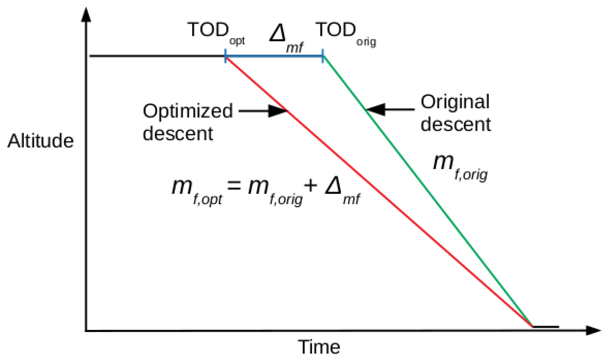
2.4.2. Flight Procedure Optimization Method

The method starts from an existing trajectory that is preferably already fuel- and noise-optimized, such as a CDA, and applies a second level of optimization to the descent phase to decrease emissions that are strongly dependent on the fuel flow. These emissions are presented in Figure 2 through their emissions indices with respect to fuel flow at sea level. In order to avoid the critical area at low idle thrust at which emissions indices exponentially increase, a minimum threshold for the fuel flow at sea level is set at 0.17 kg/s where all ${\mathrm{EIs}}_{\mathrm{sl}}$ remain below 10 g/kg. The cap of 10 g/kg has been arbitrarily chosen to limit exponential growth while minimizing the idle thrust. This means that any point along the descent phase experiencing a converted fuel flow at sea level below 0.17 kg/s is increased to that value.

A higher fuel-flow rate is thus obtained by increasing $N_1$; i.e., thrust is increased. Since either Mach number or airspeed is kept at a desired value at a given altitude during normal operations, the effect of the increased $N_1$ will lead to a reduced rate of descent. An earlier top of descent (TOD) will therefore be required, since the descent will be performed over a longer time and, therefore, also over a longer distance. A valid approximation will also be that the Mach number will be the same at any given altitude for the optimized and non-optimized trajectory. The new optimized TOD, ${\mathrm{TOD}}_{\mathrm{opt}}$, is proportionally advanced to counterbalance the additional amount of fuel resulting from the increased fuel flow; see Figure 4. The time margin between the original ${\mathrm{TOD}}_{\mathrm{orig}}$ and ${\mathrm{TOD}}_{\mathrm{opt}}$, ${\Delta }_{mf}$, corresponds to the additional energy required to optimize the original descent. The new optimized descent should then result in a total burned fuel of $m_{f,opt}=m_{f,orig}+{\Delta }_{mf}$ in order to not increase the total burned fuel and corresponding proportional emissions through the optimization. Moreover, the optimized descent profile is adapted to follow the original descent profile as closely as possible.

3. Results

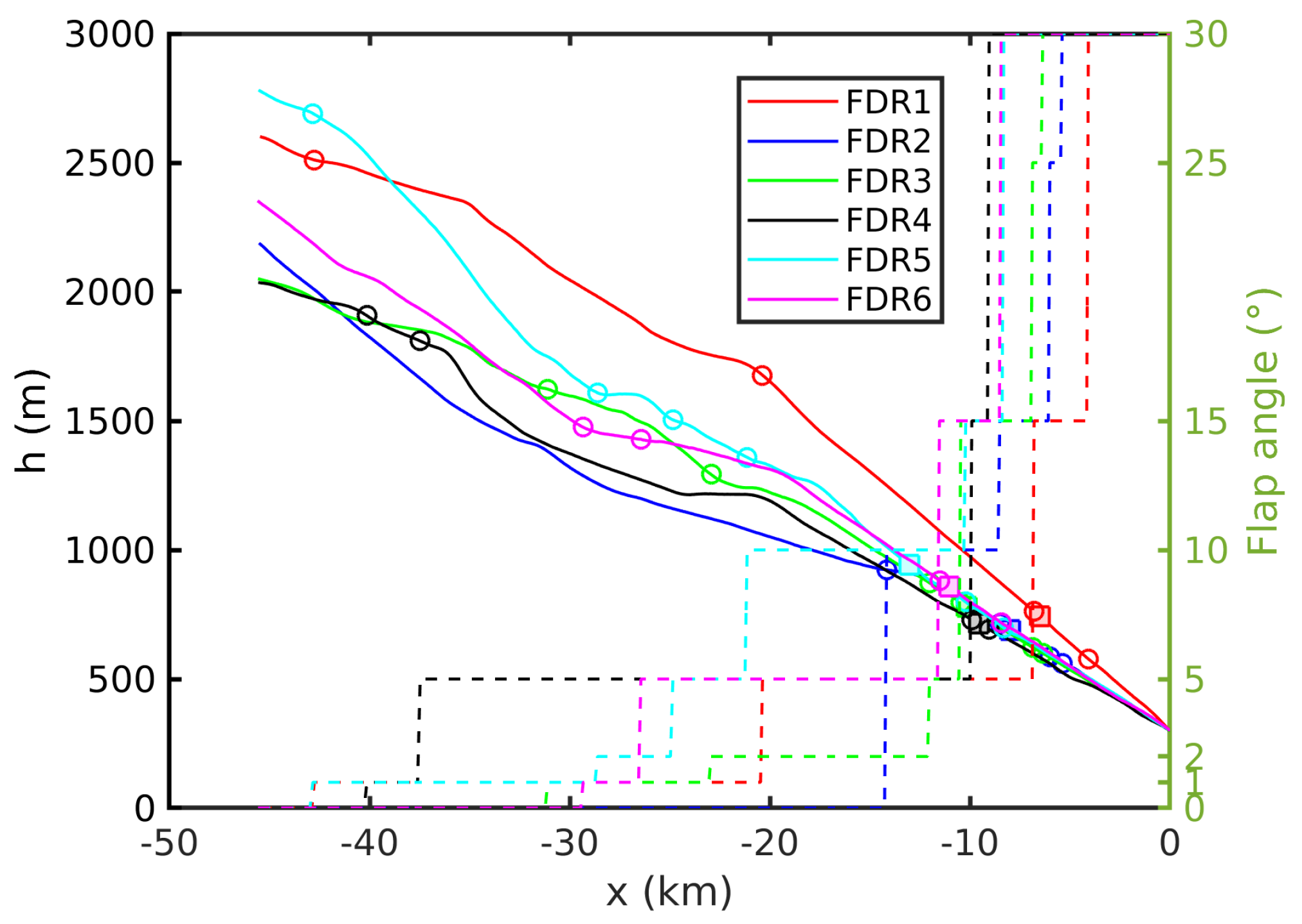
3.1. Flight Trajectories

The flight trajectories under investigation are presented in Figure 5 with their respective flight configurations in terms of flaps and landing gear. These approach trajectories have been extracted from FDR data files provided by SAS. Note that the whole analysis only considers the vertical profile of the approach trajectories and does not focus on the final approach as indicated in Figure 5. However, in terms of noise, the complete maps are displayed until touch down.

3.2. Emissions Analysis

Emissions are computed for each trajectory using the presented model in Section 2.2. Before focusing on the trajectory comparison in terms of the different gas emissions, a first look is taken at a single trajectory to analyze, compare, and understand the behavior of each of these gas emissions.

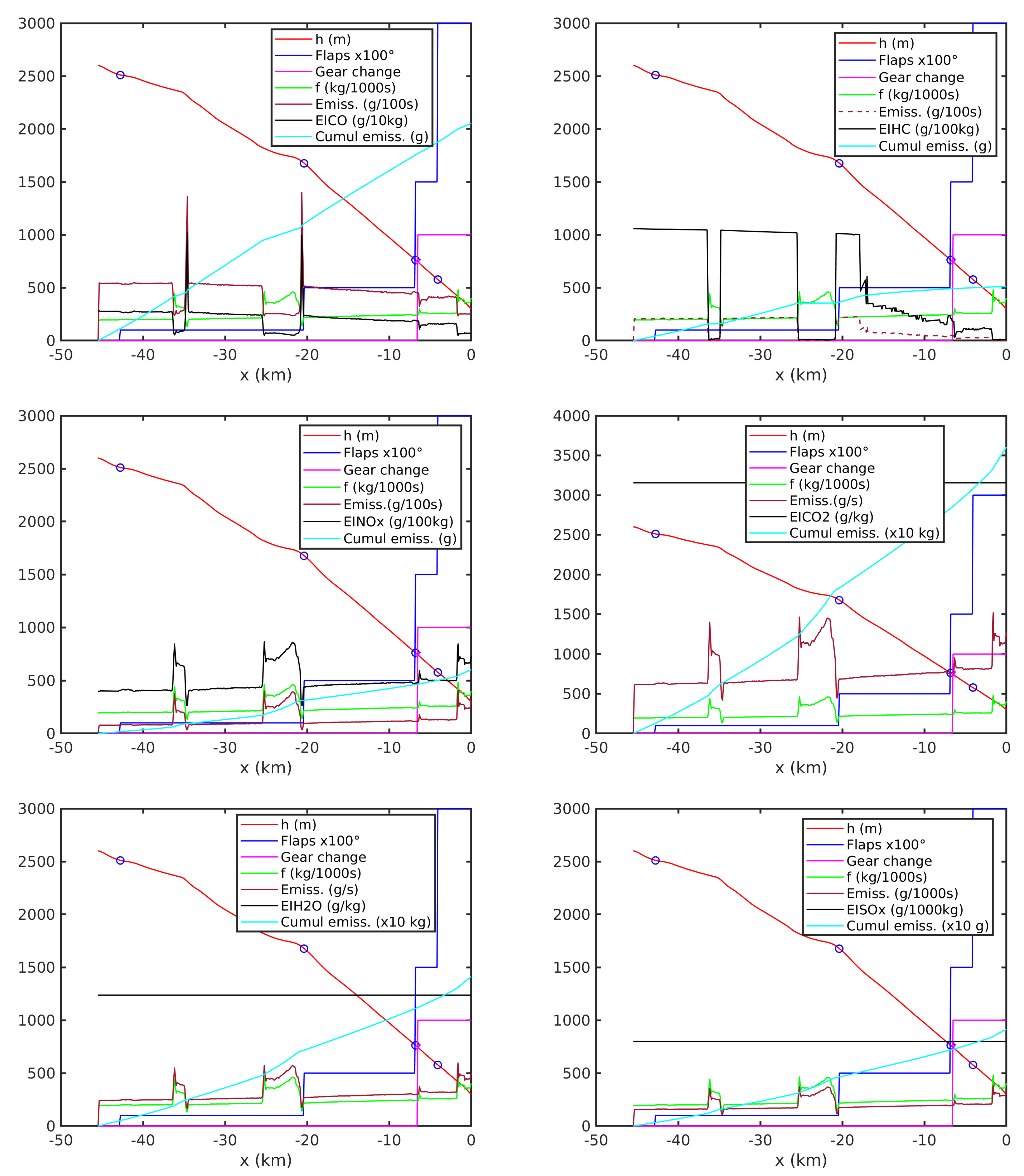
3.2.1. Single Trajectory

Figure 6 shows the evolution of $\mathrm{CO}$, $\mathrm{HC}$, ${\mathrm{NO}}_{\mathrm{x}}$, ${\mathrm{CO}}_2$, ${\mathrm{H}}_2\mathrm{O}$, and ${\mathrm{SO}}_{\mathrm{x}}$ along the approach phase of FDR1, with the different flap and landing-gear configurations indicated. In addition, the emissions are presented in three different ways, namely, the emissions in grams per second at each point of the trajectory, the cumulative emissions over the distance, and the emissions indices at altitude, which can interestingly be correlated to fuel-flow evolution at altitude.

As expected, the emissions ${\mathrm{CO}}_2$, ${\mathrm{H}}_2\mathrm{O}$, and ${\mathrm{SO}}_{\mathrm{x}}$ follow the same trend as the fuel flow, since they are proportional to the burned fuel through constant emissions indices; see Equations (1)–(3). ${\mathrm{NO}}_{\mathrm{x}}$ also experiences the same trend, since its corresponding emission index follows the fuel-flow evolution at sea level, Figure 2. On the other hand, $\mathrm{CO}$ and $\mathrm{HC}$ have an opposite trend as a consequence of their opposite emissions index evolutions at sea level with respect to fuel flow; see Figure 2.

The opposite behavior of the emissions already reflects the complexity of reducing all the gas emissions through a single optimization strategy. In addition, the atmospheric conditions that correspond in this study to the standard atmosphere and directly affect $\mathrm{CO}$, $\mathrm{HC}$, and ${\mathrm{NO}}_{\mathrm{x}}$ (Equations (4)–(6)) will be perturbed by the local weather or climate, adding a layer of uncertainty to the variation of these emissions. Therefore, it may be the case that ${\mathrm{NO}}_{\mathrm{x}}$ emissions do not evolve as ${\mathrm{CO}}_2$ for the same optimization strategy.

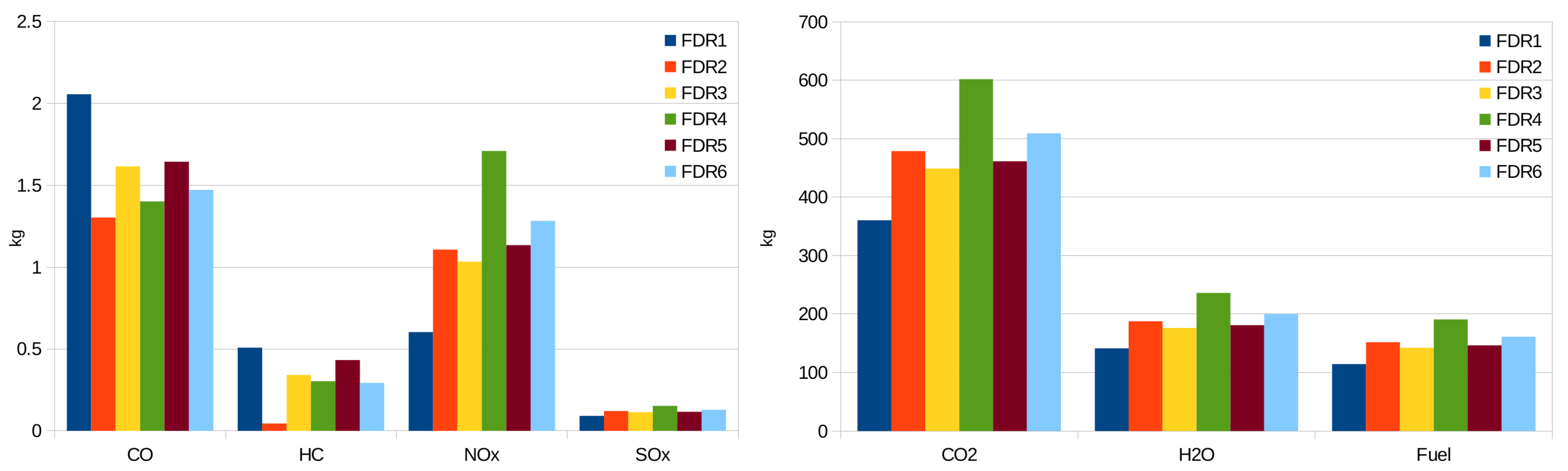
3.2.2. Trajectory Comparison

The emissions are now compared between the trajectories under investigation (Figure 5).

Table 2. Total level of emissions and burned fuel for each flight trajectory (FDR1-6).

FDR#	CO (kg)	HC (kg)	${\mathbf{NO}}_{\mathbf{x}}$ (kg)	${\mathbf{CO}}_2$ (kg)	${\mathbf{H}}_2\mathbf{O}$ (kg)	${\mathbf{SO}}_{\mathbf{x}}$ (kg)	Fuel (kg)
1	2.05	0.51	0.60	360.35	141.28	0.09	114.21
2	1.30	0.05	1.11	478.59	187.64	0.12	151.69
3	1.62	0.34	1.03	448.95	176.02	0.11	142.30
4	1.40	0.30	1.71	601.73	235.93	0.15	190.72
5	1.64	0.43	1.13	461.26	180.85	0.12	146.20
6	1.47	0.29	1.28	508.94	199.54	0.13	161.31

gives the total level of emissions for each gas emission type and per trajectory, FDR1 to FDR6. It reveals how the trajectories will favor different types of emissions, namely, emissions evolving with the fuel flow or inversely to it. For example, whereas HC and CO emissions are decreased in FDR2 by a factor of about 10 and 1.6, respectively, compared to FDR1, ${\mathrm{NO}}_{\mathrm{x}}$ is increased by a factor of almost two, and ${\mathrm{CO}}_2$, ${\mathrm{H}}_2\mathrm{O}$, and ${\mathrm{SO}}_{\mathrm{x}}$ by a factor of 1.3. A similar trend can be observed between FDR4 and FDR1, where a maximum factor ratio of 1.7 is found for ${\mathrm{CO}}_2$, ${\mathrm{H}}_2\mathrm{O}$, and ${\mathrm{SO}}_{\mathrm{x}}$ for FDR4 compared to FDR1, whereas CO and HC are almost proportionally decreased in FDR4 by 1.5 and 1.7, respectively. Figure 7 gives a better representation of the emissions comparison, and

Table 3. Ordering of the flight trajectories (FDR1-6) in terms of emissions and burned fuel from 1 (the lowest) to 6 (the highest).

FDR#	CO	HC	${\mathbf{NO}}_{\mathbf{x}}$	${\mathbf{CO}}_2$	${\mathbf{H}}_2\mathbf{O}$	${\mathbf{SO}}_{\mathbf{x}}$	Fuel
1	6	6	1	1	1	1	1
2	1	1	3	4	4	4	4
3	4	4	2	2	2	2	2
4	2	3	6	6	6	6	6
5	5	5	4	3	3	3	3
6	3	2	5	5	5	5	5

orders the trajectories with respect to their impact on the different gas emissions. Through this last table, it can be clearly identified that the trajectories most favorable for fuel-flow-“proportional” emissions reduction cause the strongest impact in terms of the inversely evolving emissions, such as FDR1 trajectory. The opposite observation applies to FDR2, followed by the FDR4 and FDR6 trajectories, which are more beneficial for CO and HC emissions. The goal would be to find a trade-off strategy to mitigate all the gas emissions in the best way possible.

A further comparison is provided in Figure 8 in terms of the emissions indices with respect to fuel flow at sea level for CO, HC, and ${\mathrm{NO}}_{\mathrm{x}}$. The idea is to reach a deeper understanding of the impact of flight procedures on emissions by visualizing the core of the problem. As can be seen, FDR1, which was ranked as the least favorable in terms of HC and CO, actually experiences very low fuel-flow levels, leading to emissions indices within the critical area of exponential growth. The uncertainty of the exponential growth, which could be indefinitely increased, is limited to the maximum value obtained in the APEX study (Section 2.2.1, Figure 2). Unfortunately, this uncertainty area will determine the actual level of emissions for CO and HC, which could strongly differ depending on where this upper limit is set. In this study, we chose to consider worst-case scenarios. On the contrary, the fact that FDR2 was most favorable for CO and HC emissions reduction (Table 3) is also reflected in Figure 8. The emissions indices are mostly concentrated at the lowest values and are, therefore, almost unaffected by the maximum limitation. Finally, FDR4’s values are between both cases, corresponding as well to the ordering in Table 3. Concerning $\mathrm{NOx}$, it can also be noticed how its emissions index values are spread from low to higher fuel-flow levels compared to FDR1 and FDR2.

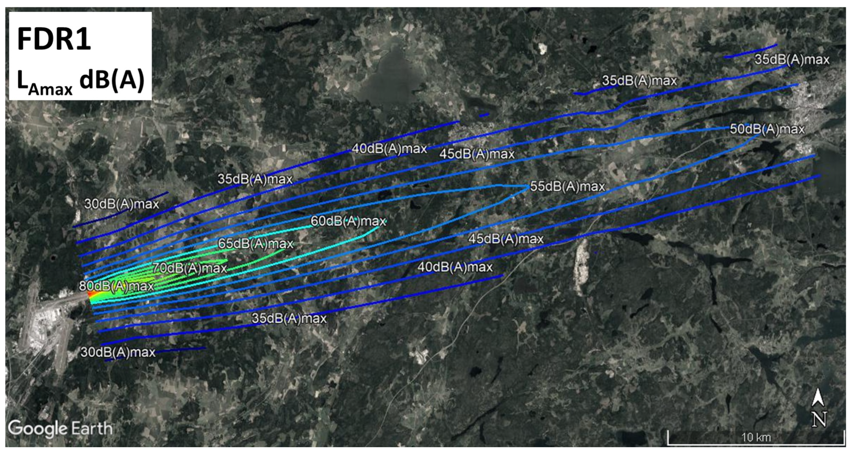
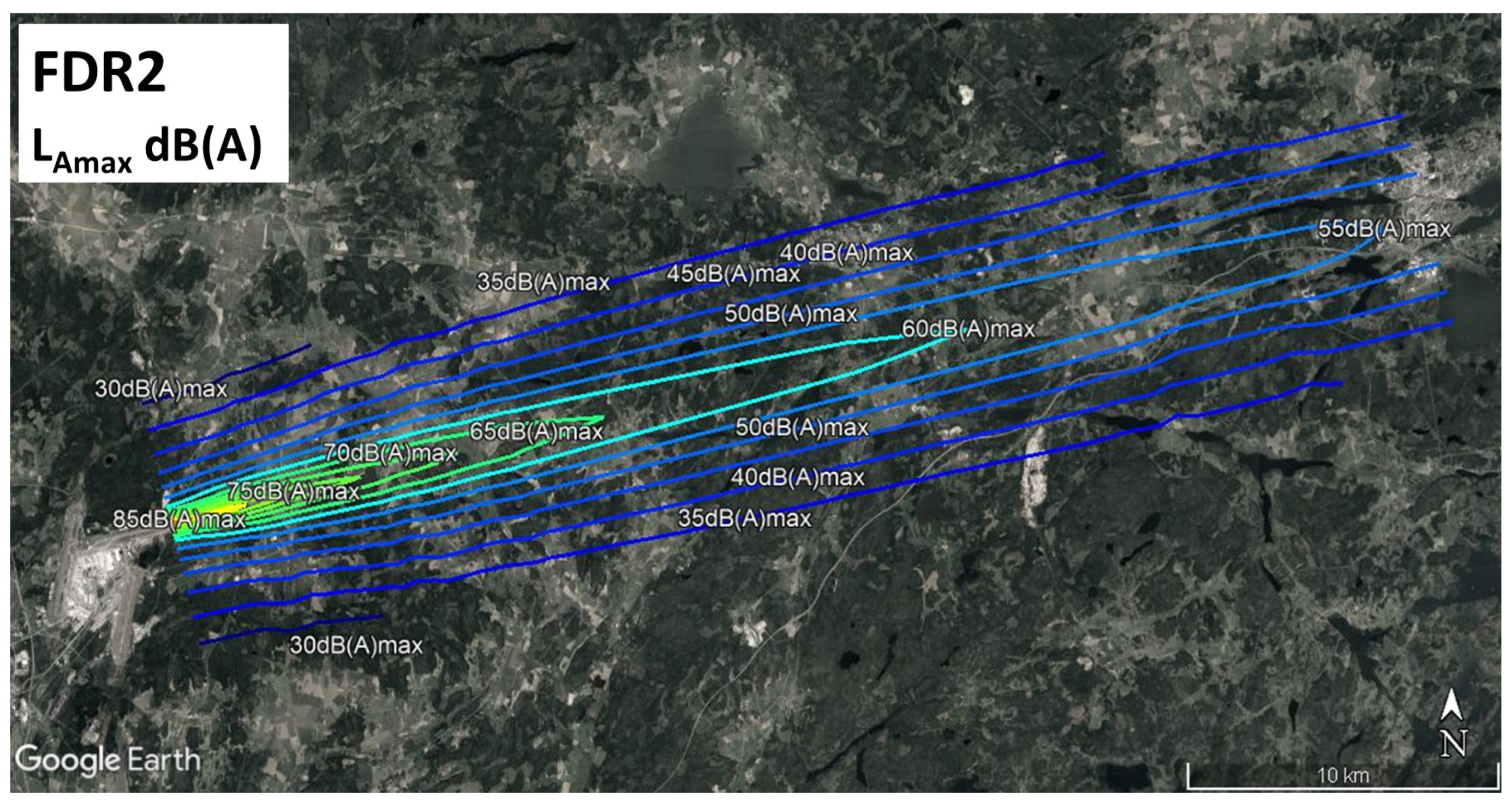
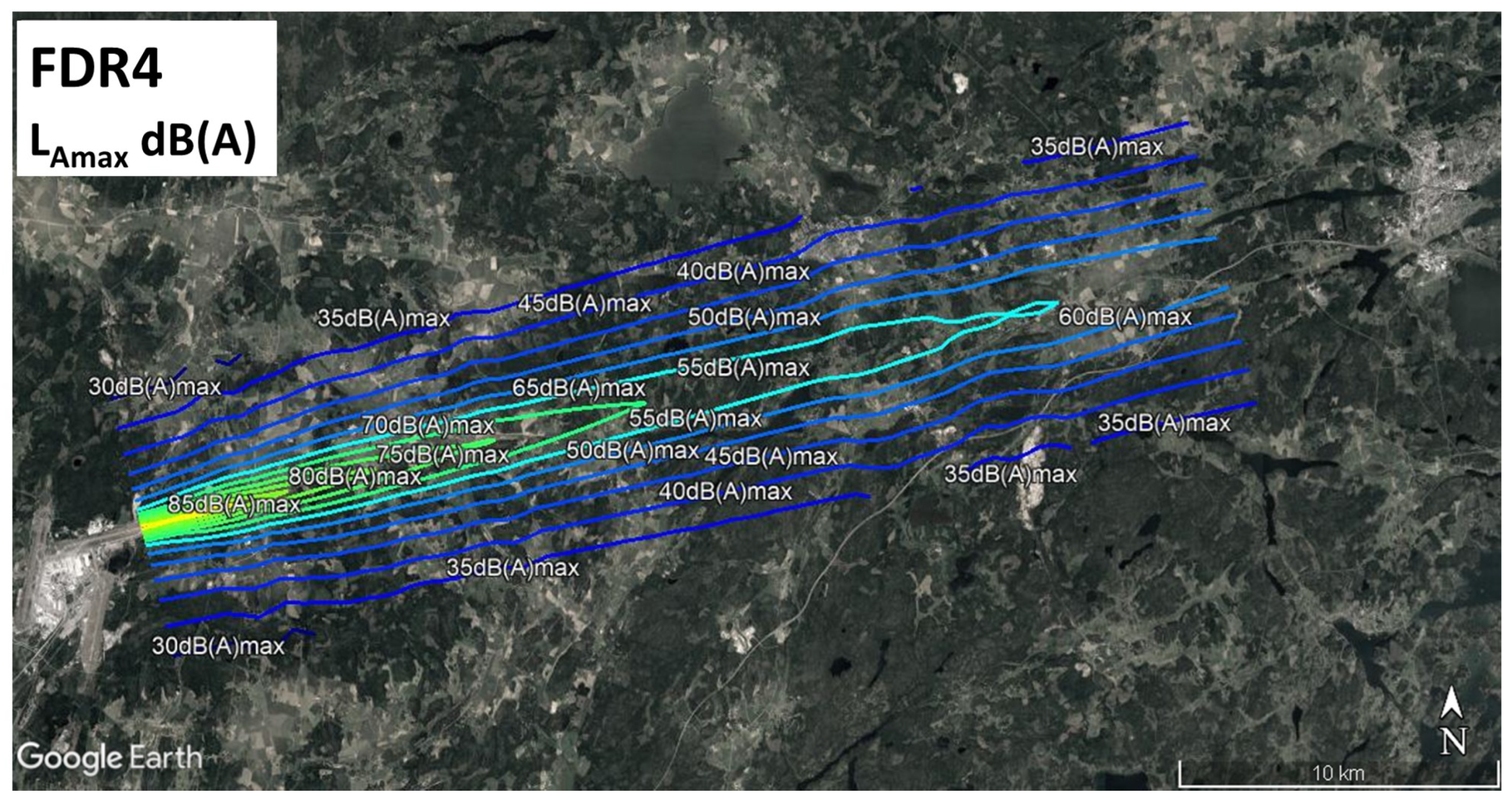
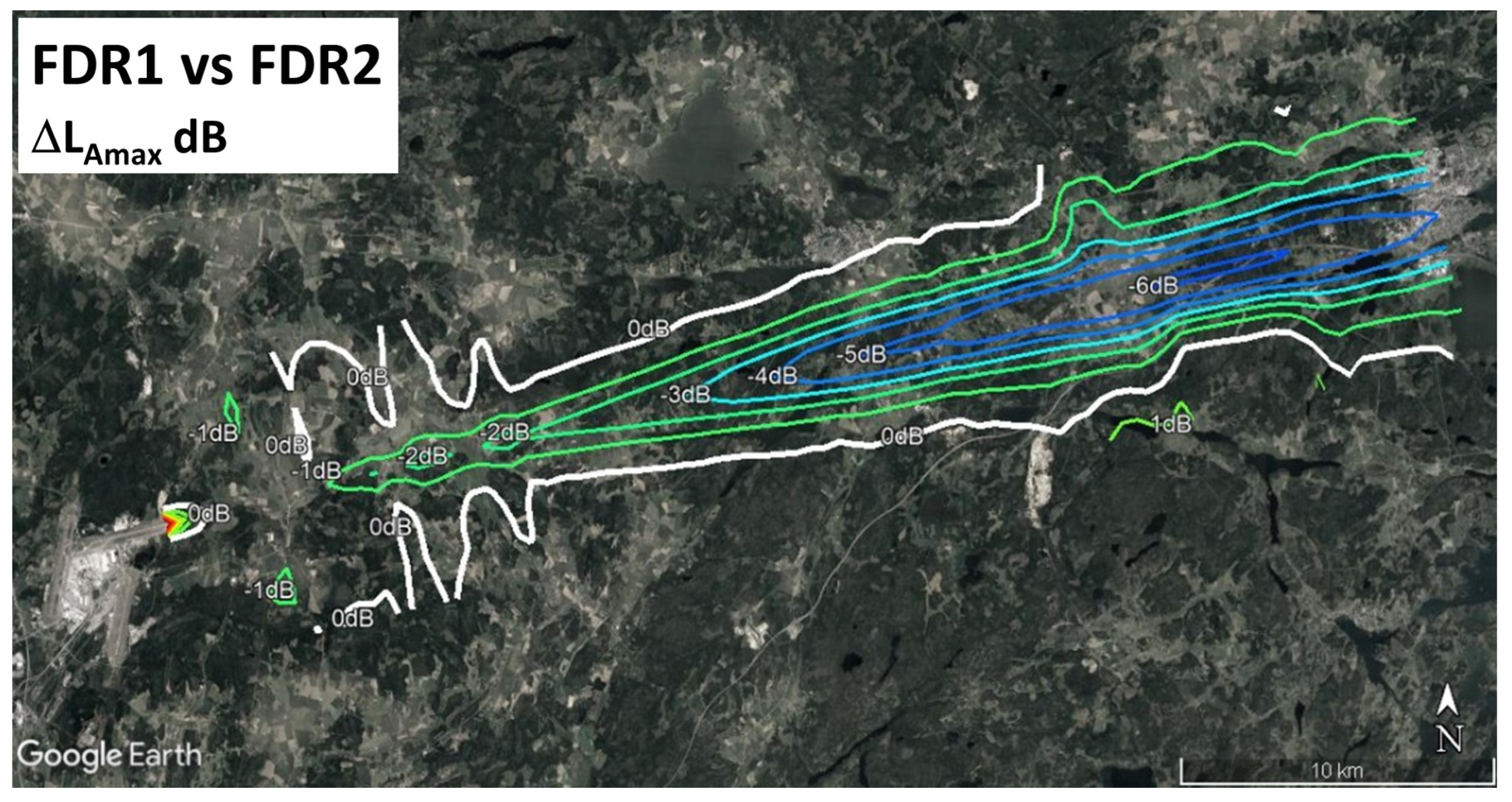
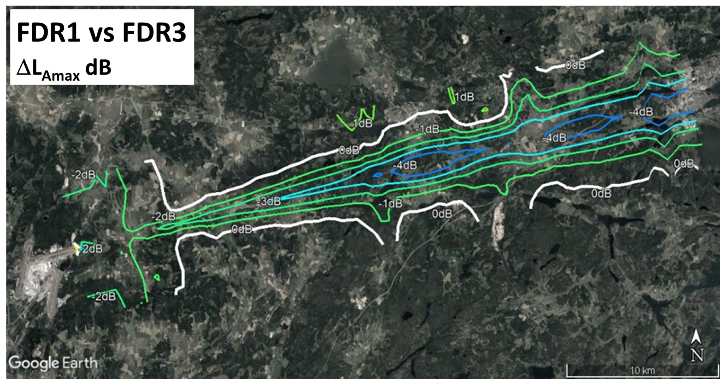
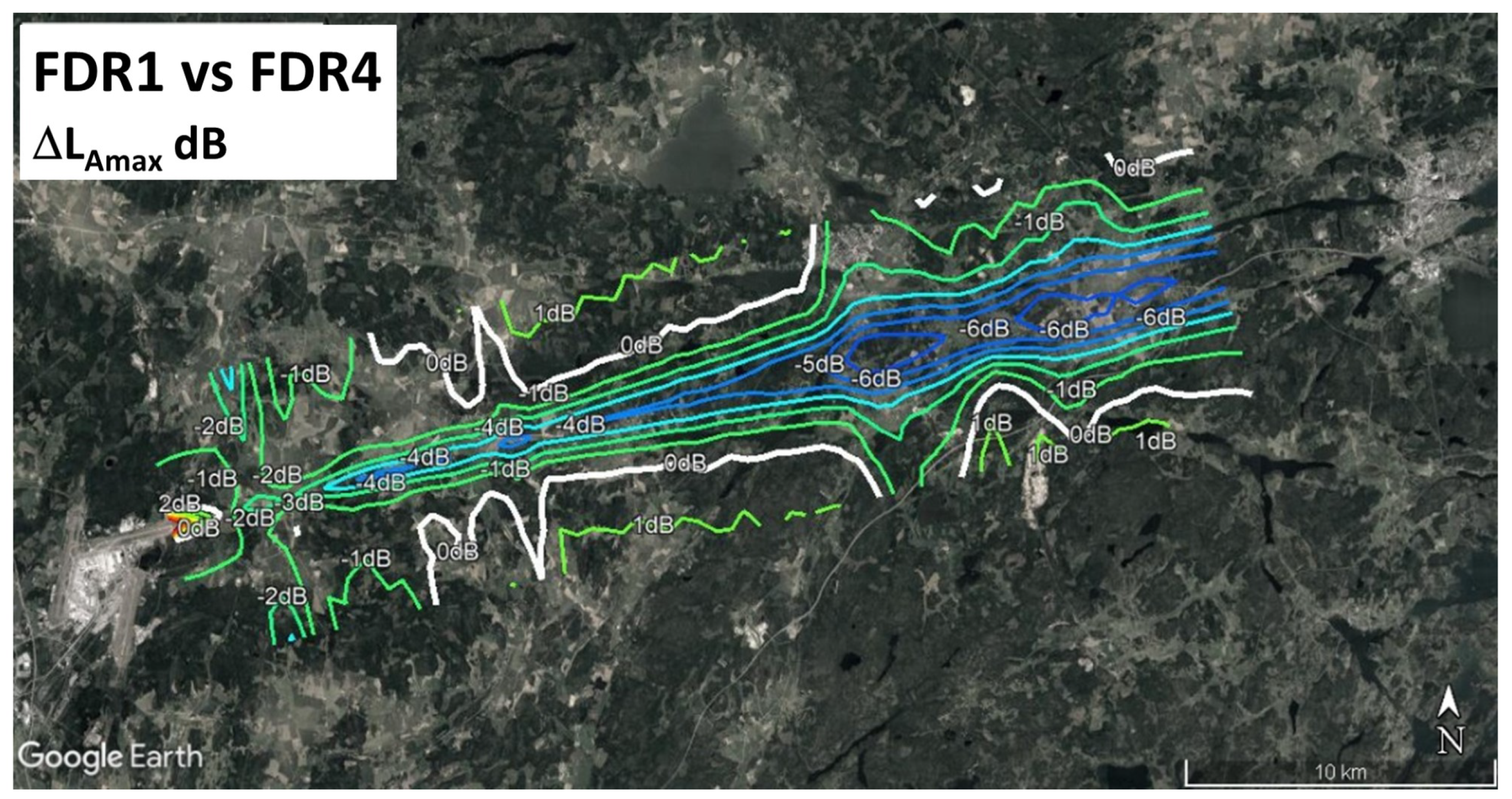
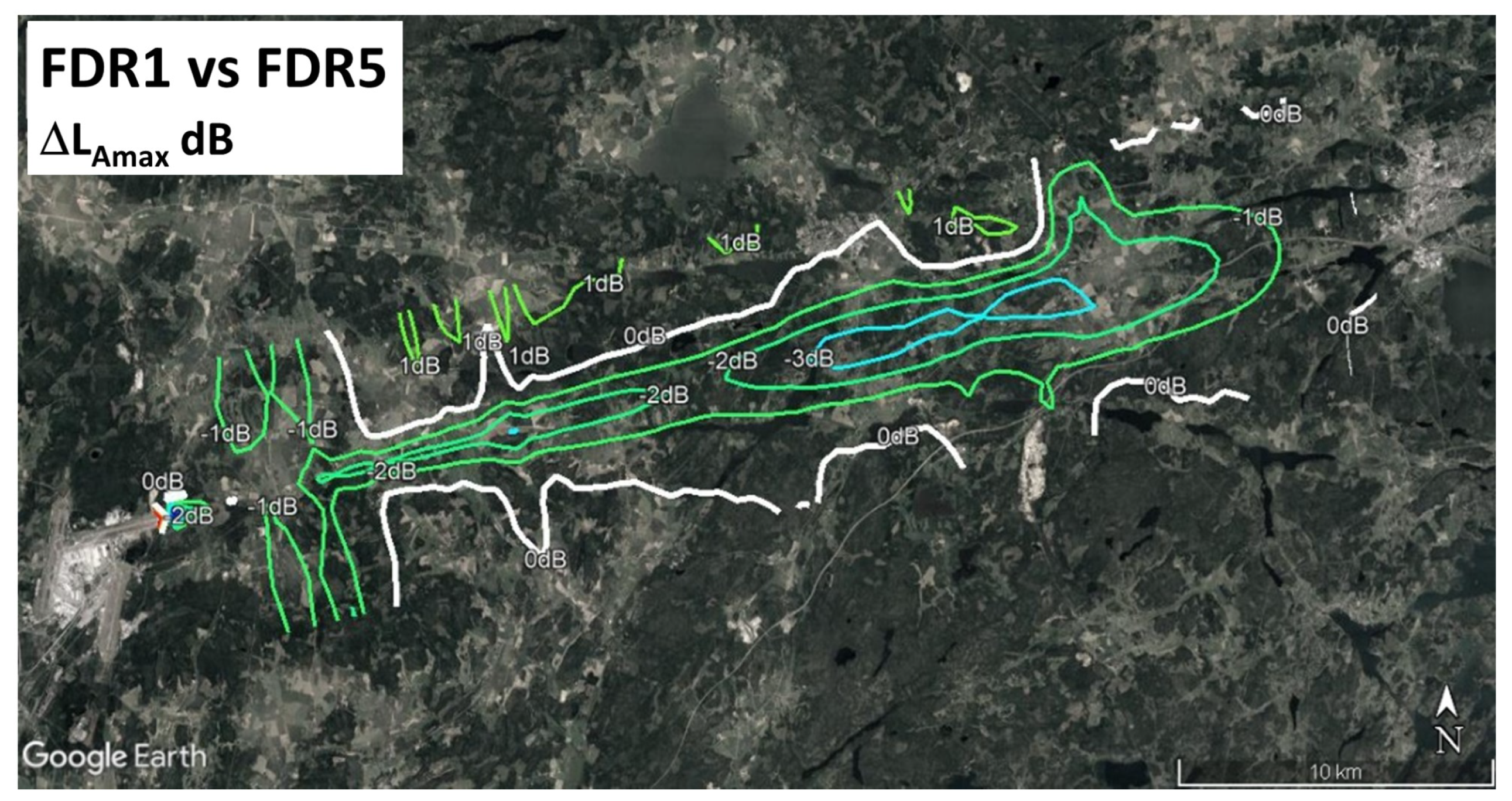
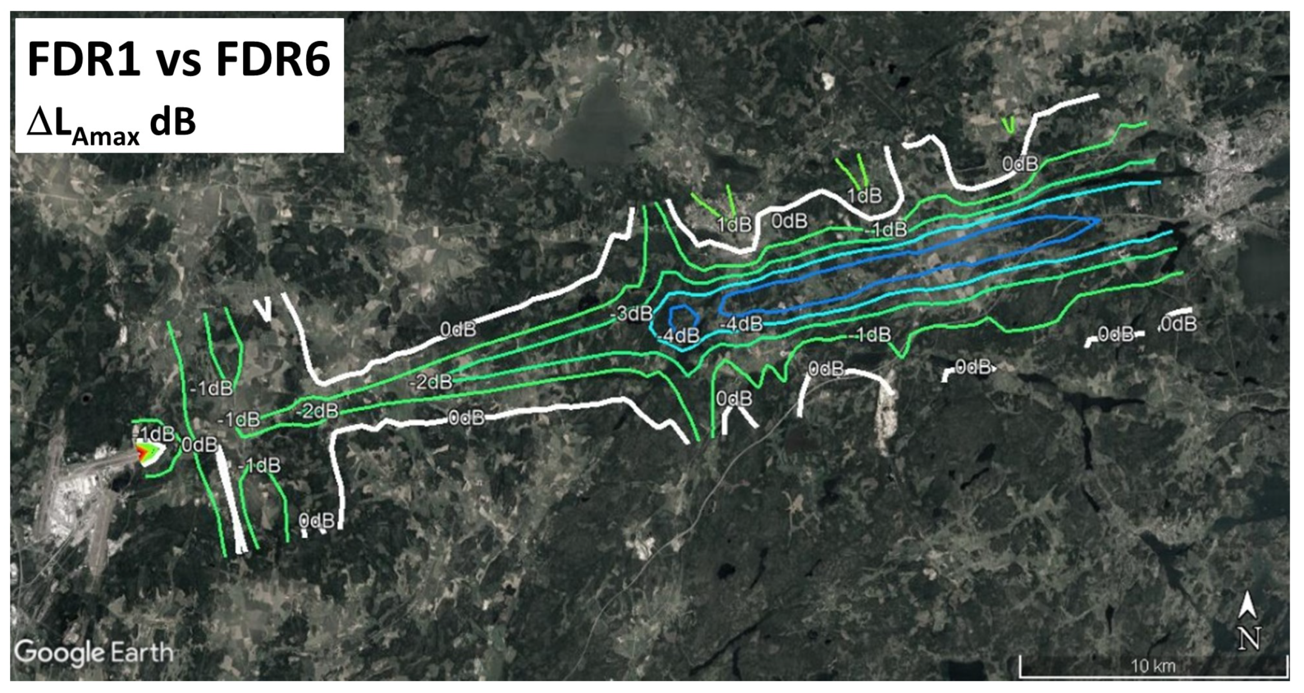
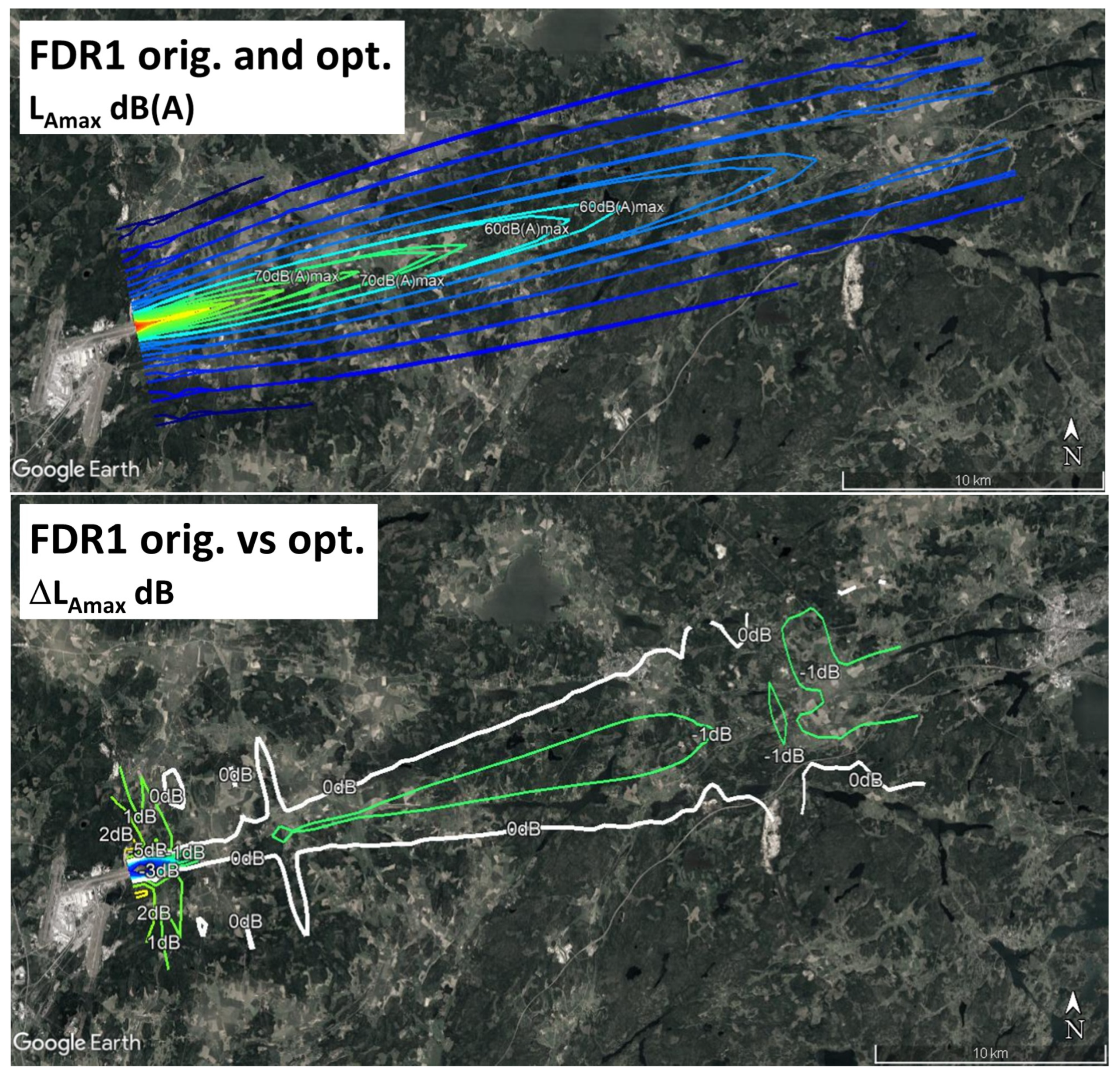
3.3. Noise Analysis and Interdependencies with Emissions

For noise prediction, the flights were assumed to be straight and were positioned in the approach phase at Arlanda Airport runway 26, in Stockholm (Sweden). Hence, the flight paths were placed in a realistic context over rather flat ground.

As could be earlier noticed, FDR1 stands out from the others due to its higher altitude (Figure 5) as well as lower thrust (Figure 8). Both indicate expected lower noise levels, confirmed by the computed noise maps below. Figure 9, Figure 10 and Figure 11 show the noise contour maps of the maximum A-weighted sound level ($L_{\mathrm{Amax}}$) for FDR1, 2, and 4, where FDR1 gives lower noise levels, e.g., with about 17 km extension of the 60 dBA contour out from the runway, compared to about 26 km for FDR2 and 30 km for FDR4. These observations can be directly related to the fuel-flow levels comparison from Figure 8, where FDR1 has the lowest fuel-flow levels, followed by FDR2 and FDR4. This last observation corresponds as well to the flight ordering presented in Table 3 in terms of the burned-fuel-dependent emissions, namely, ${\mathrm{CO}}_2$, ${\mathrm{H}}_2\mathrm{O}$, and ${\mathrm{SO}}_{\mathrm{x}}$, which are ordered 1, 4, and 6, respectively.

In order to more efficiently compare the results for the six flights, the noise impact differences between FDR1 and the other trajectories are displayed in Figure 12, Figure 13, Figure 14, Figure 15 and Figure 16. The contours display $\Delta L_{\mathrm{Amax},\mathrm{FDR}1,i}=L_{\mathrm{Amax},\mathrm{FDR}1}-L_{\mathrm{Amax},\mathrm{FDR}i}$, for $i\in \{2:6\}$, where the negative $\Delta L_{\mathrm{Amax},\mathrm{FDR}1,i}$ values indicate the lower noise impact of FDR1 with respect to each FDRi flight. With FDR4 characterized by a lower altitude (Figure 5) and higher thrust (Figure 8), we see the largest difference with respect to FDR1, as indicated in Table 3. Moreover, the difference in $L_{\mathrm{Amax}}$ levels is strongest around the ground track and more than 20 km out from the runway threshold. Since wind data is missing in these predictions, the comparison accuracy could be slightly affected.

Hence, the observations made for noise prediction are perfectly aligned with Table 3, and Figure 5, Figure 7, and Figure 8, where the flight trajectories giving the highest burned-fuel-proportional emissions, such as ${\mathrm{CO}}_2$, also result in the highest noise impact. FDR1 is, in fact, the most favorable in terms of noise and burned-fuel-proportional emissions, contrary to FDR4. Therefore, a decrease in thrust will lead to lower noise and burned fuel, thereby reducing emissions dependent on the burned fuel. The challenge now is to define a trade-off strategy considering the fuel-flow-dependent emissions, especially HC and CO.

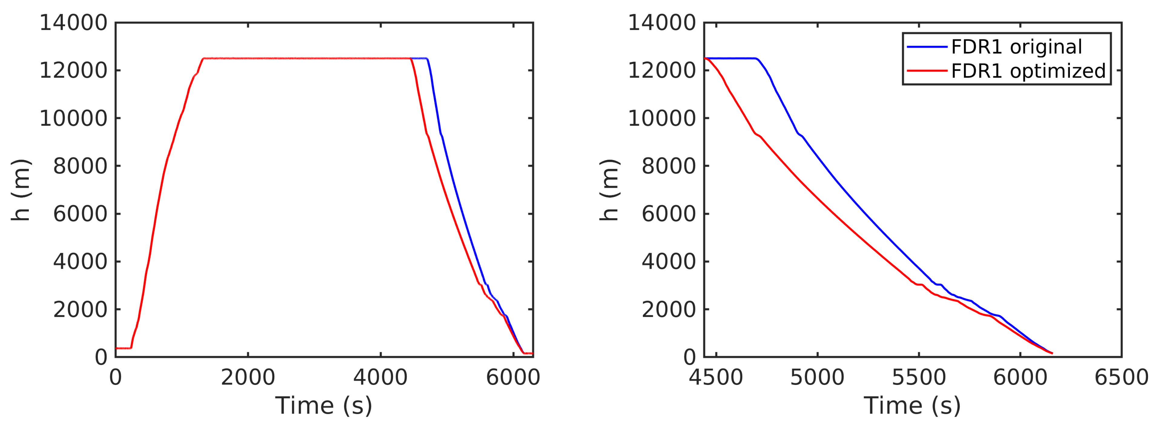
3.4. Flight Procedure Optimization

After an individual analysis of each gas emission and noise for all the presented trajectories, the final goal is to define an optimal trade-off solution in terms of flight procedures for a combined environmental impact reduction.

FDR1 has been shown to have the least noise impact due to its high altitude during the CDA approach and the lowest level of burned-fuel-proportional emissions. This flight is therefore selected as the noise- and fuel-optimized trajectory of reference to be further optimized in terms of gas emissions (Section 2.4.2). A special focus is therefore placed on minimizing HC and CO, since CDAs based on idle thrust are normally already fuel-optimal procedures and thereby minimize burned-fuel-proportional emissions, namely, ${\mathrm{CO}}_2$, ${\mathrm{H}}_2\mathrm{O}$, and ${\mathrm{SO}}_{\mathrm{x}}$ (Equations (1)–(3)).

The core of this optimization process consists in setting a minimum cap in terms of fuel flow or thrust in the flight procedure to avoid the critical area of exponential growth of CO and HC emissions; see Figure 2.

3.4.1. CO and HC Minimization

The trajectory simulation code is used to investigate the impact of the throttle setting through the $N_1$ control variable on the fuel-flow-dependent gas emissions, namely, HC, CO, and ${\mathrm{NO}}_{\mathrm{x}}$ (Equations (4)–(6)) for the FDR1 descent phase of Figure 3. By increasing $N_1$ by, for example, 12% along the trajectory where the fuel-flow rates at sea level are below 0.17 kg/s, it is possible to strongly decrease the CO and HC emissions by factors of almost 2 and 16, respectively; see

Table 4. Comparison of total level of emissions and burned fuel for the simulated FDR1 descent trajectory: original and optimized.

FDR1	CO (kg)	HC (kg)	${\mathbf{NO}}_{\mathbf{x}}$ (kg)	${\mathbf{CO}}_2$ (kg)	${\mathbf{H}}_2\mathbf{O}$ (kg)	${\mathbf{SO}}_{\mathbf{x}}$ (kg)	Fuel (kg)
Original	7.24	1.57	1.42	928.61	364.09	0.24	294.33
CO/HC-optimized	4.20	0.10	2.72	1324.03	519.12	0.34	419.66
Reduction factor	1.72	15.7	-	-	-	-	-
Increase factor	-	-	1.92	1.43	1.43	1.42	1.43

. In fact, this increase results in much lower emissions index values; see Figure 17 (bottom).

On the other hand, the same optimization would result in an increase of the ${\mathrm{NO}}_{\mathrm{x}}$ emissions by almost a factor of two since, contrary to HC and CO, the ${\mathrm{NO}}_{\mathrm{x}}$ emission index does increase with an increased fuel flow (Figure 2). Further variations could continue decreasing or increasing the mentioned emissions. Moreover, the additional amount of fuel required for this purpose will result in an increase in the total burned fuel and, consequently, in burned-fuel-proportional emissions. In this case, the amount of burned fuel and proportional emissions were increased by a factor of about 1.4 (Table 4).

3.4.2. Environmentally Optimal Trajectory

The same strategy consisting of applying a minimum threshold at sea level of 0.17 kg/s is still used here. However, we now look at the whole trajectory and aim to define an appropriate earlier ${\mathrm{TOD}}_{\mathrm{opt}}$, which would compensate for the additional fuel flow required for optimization of the descent phase (Section 2.4.2, Figure 4). Figure 18 shows both trajectories—the original FDR1 and the optimized one—to minimize not only the burned fuel and the resulting dependent emissions ${\mathrm{CO}}_2$, ${\mathrm{H}}_2\mathrm{O}$, ${\mathrm{SO}}_{\mathrm{x}}$, and ${\mathrm{NO}}_{\mathrm{x}}$, but also the inversely fuel-flow-dependent emissions HC and CO. Note that for this optimization study, emissions are computed for the FDR1 trajectories, original and optimized, from Figure 18 (right).

The resulting emissions are presented in

Table 5. Comparison of total level of emissions and fuel burned for FDR1 trajectory: original and optimized.

FDR1	CO (kg)	HC (kg)	${\mathbf{NO}}_{\mathbf{x}}$ (kg)	${\mathbf{CO}}_2$ (kg)	${\mathbf{H}}_2\mathbf{O}$ (kg)	${\mathbf{SO}}_{\mathbf{x}}$ (kg)	Fuel (kg)
Original	9.41	2.19	2.80	1306.56	512.27	0.33	414.12
Optimized	6.61	0.52	2.40	1307.33	512.57	0.33	414.37
Reduction factor	1.42	4.21	1.17	∼1	∼1	1	∼1

, which shows that while maintaining the same amount of burned fuel and related emissions, it is possible to decrease CO and HC by factors of 1.4 and 4.2, respectively. In fact, Figure 19 (bottom) shows lower levels of corresponding emissions indices at sea level.

Moreover, the noise impact of the new FDR1 optimized trajectory should also be assessed to ensure optimal noise levels are still preserved in the global environmental impact assessment. As stated earlier, the FDR1 trajectory was also selected in this optimization process for its minimum noise impact compared to the other trajectories. As expected, the noise pattern in terms of $L_{\mathrm{Amax}}$ (Figure 20 (bottom)) shows a slight increase in noise level for FDR1 of 1 dB close to the ground track, i.e., a small rise in noise that, according to the (simplified) ECAC Doc 29 model, can be attributed partly to the increased thrust and partly to the lower altitude given by the optimized trajectory. In Figure 20 (top), where the two FDR1 noise contour patterns are superimposed, we may notice a distance of about 2 km between the two 60 dB(A) contours, with a smaller shift in the distance for the other constant contour levels along the ground track. Moreover, one should note that the configuration changes along the approach, which each leading to higher drag and therefore thrust required, are supposed to take place at the same latitude and longitude coordinates along the track in both studied cases.

4. Conclusions

Different flight approach trajectories were analyzed and compared in terms of noise and gas emissions impact. ${\mathrm{CO}}_2$ and non-${\mathrm{CO}}_2$ emissions were individually investigated based on their emission index with respect to fuel flow at sea level, revealing their interdependencies. It was shown that the most favorable trajectories for the reduction of noise and emissions evolving with fuel flow (${\mathrm{NO}}_{\mathrm{x}}$) or proportional to the burned fuel, such as ${\mathrm{CO}}_2$, resulted in worst-case scenarios for emissions that evolve inversely with respect to fuel flow, namely CO and HC. The emissions indices of these latter experience, in fact, exponential growth at very low idle thrust. It was observed that all the approach trajectories analyzed were in this area of exponential growth. A trade-off optimization solution was derived by setting a minimum cap for idle-thrust level at sea level on the most favorable trajectory for noise and ${\mathrm{CO}}_2$ emissions reduction—FDR1. This cap would prevent the critical area of exponential growth of both CO and HC emissions from being reached. With this approach and the resulting new optimized trajectory, CO and HC emissions could be reduced by a factor of at least 1.4 and 4.2, respectively, for a similar level of minimum noise and burned fuel, and thereby burned-fuel-proportional emissions (${\mathrm{CO}}_2$, ${\mathrm{SO}}_{\mathrm{x}}$, ${\mathrm{H}}_2\mathrm{O}$). If burned fuel or noise minimization during the approach are not considered, HC emissions could be reduced by a factor of at least 16. Removing the maximum cap on the exponential increase of the HC emission index with respect to fuel flow would lead to a higher HC emission level for the non-optimized trajectory, resulting in an even greater reduction factor than 16.

Hence, optimizing flight procedures for combined environmental impact reduction was shown to be challenging. The complex interdependencies between the different environmental variables may not follow the same trend, but rather, an opposite one, such as HC and CO emissions compared to ${\mathrm{NO}}_{\mathrm{x}}$, as well as ${\mathrm{CO}}_2$, ${\mathrm{SO}}_{\mathrm{x}}$, and ${\mathrm{H}}_2\mathrm{O}$. This phenomenon shows that by focusing only on ${\mathrm{CO}}_2$ emissions or fuel reduction, or even ${\mathrm{NO}}_{\mathrm{x}}$, new flight procedures could unexpectedly lead to a significant increase of other non-${\mathrm{CO}}_2$ emissions. An example may be the case of CDAs, which commonly use low idle thrust to decrease fuel burn without considering the exponential growth of HC and CO emissions. Additionally, there is a relevant modeling uncertainty associated with EIHC and EICO below the 7% engine power setting. Moreover, further data below this setting are not provided in the ICAO Aircraft Engine Emissions Databank. Therefore, the concern that may be raised is for how long these emissions exponentially grow for low idle-thrust levels below 7%, which must be known for accurate prediction. Additional measurements for engine thrust levels below 7% should be considered.

Independent of the emissions prediction accuracy, the simple fact that an exponential increase occurs reinforces the need for a minimum threshold for idle thrust during the approach phase to prevent the pilot from reaching the critical exponential growth area. The proposed method could be applied in the optimization process of the operational flight plans in the pre-tactical phase, in combination with fuel and, or noise optimization. Moreover, during the tactical phase, the pilot could also be advised to respect a minimum $N_1$ during descent. Since there is not enough data available for each engine, a minimum threshold could be set by default at 7% engine power, for which ICAO provides emissions data. Based on the environmental complexity highlighted, especially in terms of gas emissions, different indicators could be defined depending on whether the environmental focus is more climate-, air quality-, or noise-oriented.

As future work, the inclusion of meteorology in the optimization process would be highly relevant, due to the strong dependency of some of the non-${\mathrm{CO}}_2$ emissions on atmospheric properties. The same applies to noise prediction, which should also include meteorological data (e.g., wind). In addition, an improved model, such as a full noise simulation approach with SAFT or a similar tool, could be used, allowing for more accurate noise source models and inputs. Moreover, decreasing noise could also result in higher ${\mathrm{CO}}_2$ emissions due, for example, to circumnavigating residential areas. In this case, the lateral profile should also be considered for a complete analysis. Finally, the use of optimized fuel flow during the approach phase should also be studied for more aircraft types when flaps and landing gear are extended. Different aircraft types have different limitations on minimum idle $N_1$ when flaps and, or landing gear are extended.

References

1. Zellmann, C.; Schaffer, B.; Wunderli, J.M.; Isermann, U.; Paschereit, C. Aircraft Noise Emission Model Accounting for Aircraft Flight Parameters. J. Aircr. 2017, 55, C034275. [Google Scholar] [CrossRef]
2. Meister, J.; Schalcher, S.; Wunderli, J.-M.; Jager, D.; Zellmann, C.; Schaffer, B. Comparison of the Aircraft Noise Calculation Programs sonAIR, FLULA2 and AEDT with Noise Measurements of Single Flights. Aerospace 2021, 8, 388. [Google Scholar] [CrossRef]
3. Tengzelius, U.; Johansson, A.; Åbom, M.; Bolin, K. Next Generation Aircraft Noise-Mapping. In Proceedings of the INTER-NOISE and NOISE-CON Congress and Conference Proceedings, InterNoise21, Washington, DC, USA, 1–5 August 2021; pp. 1945–2948. [Google Scholar]
4. European Commission. Reducing Emissions from Aviation. 2020. Available online: https://ec.europa.eu/clima/policies/transport/aviation_en (accessed on 1 July 2020).
5. EASA. Emissions. 2020. Available online: https://www.easa.europa.eu/eaer/topics/overview-aviation-sector/emissions (accessed on 1 July 2020).
6. Jardine, C.N. Calculating the Environmental Impact of Aviation Emissions; Oxford University Centre for the Environment: Oxford, UK, 2005. [Google Scholar]
7. Lee, D.S.; Fahey, D.W.; Skowron, A.; Allen, M.R.; Burkhardt, U.; Chen, Q.; Doherty, S.J.; Freeman, S.; Forster, P.M.; Fuglestvedt, J.; et al. A Gettelman The Contribution of Global Aviation to Anthropogenic Climate Forcing for 2000 to 2018. Atmos. Environ. 2021, 244, 117834. [Google Scholar] [CrossRef] [PubMed]
8. Grobler, C.; Wolfe, P.J.; Dasadhikari, K.; Dedoussi, I.C.; Allroggen, F.; Speth, R.L.; Barrett, S.R. Marginal Climate and Air Quality Costs of Aviation Emissions. Environ. Res. Lett. 2019, 14, 114031. [Google Scholar] [CrossRef]
9. European Council. Paris Agreement on Climate Change. 2020. Available online: https://www.consilium.europa.eu/en/policies/climate-change/paris-agreement/ (accessed on 1 July 2020).
10. ICAO (International Civil Aviation Organization). Operational Opportunities to Reduce Fuel Burn and Emissions; Document 10013; International Civil Aviation Organization: Montreal, QC, Canada, 2014. [Google Scholar]
11. Hwang, J.-H.; Lee, T.-G.; Hwang, S.-S. A Study of Optimized Operation for CO2 Emission and Aircraft Fuel Reduced Operation Procedures. J. Korean Soc. Aviat. Aeronaut. 2013, 21, 62–70. [Google Scholar] [CrossRef] [Green Version]
12. Hamy, A.; Mendoza, A.M.; Botez, R. Flight Trajectory Optimization to Reduce Fuel Burn and Polluting Emissions Using a Performance Database and ANT Colony Optimization Algorithm, AEGATS ’16 Advanced Aircraft Efficiency in a Global Air Transport System; Espace Publications: Westmount, QC, Canada, 2016. [Google Scholar]
13. Serafino, G. Multi-objective Aircraft Trajectory Optimization for Weather Avoidance and Emissions Reduction. In Modelling and Simulation for Autonomous Systems, MESAS 2015; Lecture Notes in Computer Science; Springer: Berlin/Heidelberg, Germany, 2015; p. 9055. [Google Scholar]
14. Lindner, M.; Rosenow, J.; Fricke, H. Aircraft Trajectory Optimization with Dynamic Input Variables. CEAS Aeronaut. J. 2020, 11, 321–331. [Google Scholar] [CrossRef]
15. Matthes, S.; Lührs, B.; Dahlmann, K.; Grewe, V.; Linke, F.; Yin, F.; Shine, K.P. Climate-Optimized Trajectories and Robust Mitigation Potential: Flying ATM4E. Aerospace 2020, 7, 156. [Google Scholar] [CrossRef]
16. Koenig, R.; Macke, O. Evaluation of Simulator and Flight Tested Noise Abatement Approach Procedures. In Proceedings of the 26th International Congress of the Aeronautical Sciences, Anchorage, AK, USA, 14–19 September 2008. [Google Scholar]
17. Strumpfel, C.; Hubner, J. Aircraft Noise Modeling of Departure Flight Events Based on Radar Tracks and Actual Aircraft Performance Parameters; DAGA Jahrestagung für Akustik: Hamburg, Germany, 2020; Volume 6, p. 19. [Google Scholar]
18. Filippone, A. Steep-Descent Maneuver of Transport Aircraft. J. Aircr. 2007, 44, 1727–1739. [Google Scholar] [CrossRef]
19. Kim, B.; Rachami, J. Aircraft Emissions Modeling under Low Power Conditions. In Proceedings of the A & WMA’s 101st Annual Conference and Exhibition, Portland, OR, USA, 24–27 June 2008. [Google Scholar]
20. DuBois, D.; Paynter, G.C. Fuel Flow Method 2 for Estimating Aircraft Emissions; Technical Paper Series 2006-01-1987; SAE Publications: Washington, DC, USA, 2006. [Google Scholar]
21. ICAO Aircraft Engine Emissions Databank. 2022. Available online: https://www.easa.europa.eu/domains/environment/icao-aircraft-engine-emissions-databank (accessed on 15 June 2022).
22. Wey, C.C.; Anderson, B.E.; Wey, C.; Miake-Lye, R.C.; Whitefield, P.; Howard, R. Aircraft Particle Emissions eXperiment (APEX); NASA/TM 2006-214382; ARC (Aerospace Research Center): Columbus, OH, USA, 2006. [Google Scholar]
23. Hadaller, O.J.; Momenthy, A.M. The Characteristics of Future Fuels; Boeing Publication D6–54940; SAGE Publications: New York, NY, USA, 1989. [Google Scholar]
24. Schaefer, M.; Bartosch, S. Overview on Fuel Flow Correlation Methods for the Calculation of NOx, CO and HC Emissions and Their Implementation into Aircraft Performance Software; Technical Report; DLR: Köln, Germany, 2013. [Google Scholar]
25. Otero, E.; Ringertz, U. Case Study on the Environmental Impact and Efficiency of Travel. CEAS Aeronaut. J. 2021, 13, 163–180. [Google Scholar] [CrossRef]
26. Federal Aviation Administration (FAA). Emissions and Dispersion Modeling System (EDMS) User’s Manual; Version 5; Federal Aviation Administration: Washington, DC, USA, 2007.
27. Aviation Environmental Design Tool (AEDT). 2022. Available online: https://aedt.faa.gov/ (accessed on 15 June 2022).
28. ECAC. ECAC.CEAC Doc 29, 4th ed.; Report on Standard Method of Computing Noise Contours around Civil Airports, Technical Guide; ECAC: Neuilly-sur-Seine, France, 2016; Volume 2. [Google Scholar]
29. SAE-AIR-1845; Procedure for the Calculation of Airplane Noise in the Vicinity of Airports. SAE Publications: Newbury Park, CA, USA, 1986.
30. EUROCONTROL. The Aircraft Noise and Performance (ANP) Database. 2022. Available online: https://www.aircraftnoisemodel.org/ (accessed on 4 July 2022).
31. ISO 9613-1; Acoustics—Attenuation of Sound during Propagation Outdoors—Part 1: Calculation of the Absorption of Sound by the Atmosphere. International Organization for Standardization: Geneva, Switzerland, 1993.
32. ANSI/ASA S1.26-2014; Methods for Calculation of the Absorption of Sound by the Atmosphere. American National Standards Institute: Washington, DC, USA, 2014.
33. SAE-ARP-5534; Aerospace Recommended Practice, Application of Pure-Tone Atmospheric Absorption Losses to One-Third Octave-Band Level. SAE Publications: Newbury Park, CA, USA, 2013.
Figure 1. Boeing Fuel Flow Method 2 process applied for emissions computation.
Aerospace 09 00683 g001
Figure 2. Modeling of emissions indices at sea level for the CFM56-7B27 engine based on the ICAO emissions data points adjusted for installation effects (*), and the APEX data for a similar engine (CFM56-2-C1).
Aerospace 09 00683 g002
Figure 3. Validation of the aircraft trajectory simulation code for the descent phase. Comparison between simulated and FDR data.
Aerospace 09 00683 g003
Figure 4. Optimization of descent trajectory with increased fuel flow.
Aerospace 09 00683 g004
Figure 5. Flight trajectories for the approach phase with respect to distance to final approach with flap configuration changes (circles) and corresponding angles (dashed lines), and landing-gear-down configuration (squares).
Aerospace 09 00683 g005
Figure 6. Emissions evolution along a flight trajectory (FDR1) for CO , HC , NO x , CO 2 , H 2 O , and SO x from top to bottom and left to right with respect to distance to final approach.
Aerospace 09 00683 g006
Figure 7. Emissions comparison for all the trajectories (FDR1-6).
Aerospace 09 00683 g007
Figure 8. Emissions indices at sea level with respect to fuel flow at sea level for FDR1 (top), FDR2 (middle) and FDR4 (bottom).
Aerospace 09 00683 g008
Figure 9. Noise prediction for FDR1 computed with SAFT ECAC Doc 29 implementation.
Aerospace 09 00683 g009
Figure 10. Noise prediction for FDR2 computed with SAFT ECAC Doc 29 implementation.
Aerospace 09 00683 g010
Figure 11. Noise prediction for FDR4 computed with SAFT ECAC Doc 29 implementation.
Aerospace 09 00683 g011
Figure 12. Noise prediction difference of FDR1 with respect to FDR2 using SAFT ECAC Doc 29 implementation.
Aerospace 09 00683 g012
Figure 13. Noise prediction difference of FDR1 with respect to FDR3 using SAFT ECAC Doc 29 implementation.
Aerospace 09 00683 g013
Figure 14. Noise prediction difference of FDR1 with respect to FDR4 using SAFT ECAC Doc 29 implementation.
Aerospace 09 00683 g014
Figure 15. Noise prediction difference of FDR1 with respect to FDR5 using SAFT ECAC Doc 29 implementation.
Aerospace 09 00683 g015
Figure 16. Noise prediction difference of FDR1 with respect to FDR6 using SAFT ECAC Doc 29 implementation.
Aerospace 09 00683 g016
Figure 17. Emissions indices at sea level with respect to fuel flow at sea level for the simulated FDR1 descent trajectory: original (top) and optimized (bottom).
Aerospace 09 00683 g017
Figure 18. FDR1 trajectory: original and optimized for the descent phase. Optimization including CO and HC emissions.
Aerospace 09 00683 g018
Figure 19. Emissions indices at sea level with respect to fuel flow at sea level for FDR1 trajectory: original (top) and optimized (bottom).
Aerospace 09 00683 g019
Figure 20. FDR1 original and optimized L Amax noise contours. Superimposed absolute levels (top) and level differences (bottom).
Aerospace 09 00683 g020