Backstepping- and Sliding Mode-Based Automatic Carrier Landing System with Deck Motion Estimation and Compensation

Abstract

This paper addresses the automatic carrier landing problem in the presence of deck motion, carrier airwake disturbance, wind shears, wind gusts, and atmospheric turbulences. By transforming the 6-DOF aircraft model into an affine dynamic with angle of attack controlled by thrust, the equations associated to the resultant disturbances are deduced; then, a deck motion prediction block (based on a recursive-least squares algorithm) and a tracking differentiator-based deck motion compensation block are designed. After obtaining the aircraft reference trajectory, the backstepping control method is employed to design a novel automatic carrier landing system with three functional parts: a guidance control system, an attitude control system, and an approach power compensation system. The design of the attitude subsystem involves the flight path control, the control of the attitude angles, and the control of the angular rates. To obtain convergence performance for the closed-loop system, the backstepping technique is combined with sliding mode-based command differentiators for the computation of the virtual commands and extended state observers for the estimation of the disturbances. The global stability of the closed-loop architecture is analyzed by using the Lyapunov theory. Finally, simulation results verify the effectiveness of the proposed carrier landing system, the aircraft reference trajectory being accurately tracked.

1. Introduction

Carrier landing requires skills from the pilot because this landing process is characterized by the simultaneous movement of aircraft and carrier ship. The pilot should bring the airplane to a certain point on the ship; if it lands before the desired point, a crash into the stern is possible; on the contrary, if the landing on the carrier is too long, the pilot must take off and try again. The landing phase on carrier ships is also difficult because of the small size of the ideal landing area (e.g., width: 16.76 m and length: 12.19 m for CVN-65 Enterprise carrier). Deviation from this desired landing area (the so-called “landing box”) can lead to a collision with other aircraft parked on the carrier ship. Another difficulty of the landing process on aircraft carriers is related to the deviation angle of the runway in relation to the longitudinal axis of the ship, which is 9° [1]. Due to the restrictions caused by the optimal landing area and the short length of the runway, the aircraft should track a predefined landing path with a very small margin of error, while maintaining a constant attack angle and velocity. The efficiency of the aerodynamic surfaces is low because of the low speed and the high attack angle. The motion of the carrier deck makes the process even more difficult as the desired landing path and the point of contact move with the runway. The landing process is also difficult because the aircraft descends on a slope that is not aligned with the longitudinal axis of the runway.

The need of automatic carrier landing control systems (ACLSs) is due not only to the positioning errors that should be very small but also to the weather conditions. Therefore, the flight officers who monitor the landing process are very strict when it comes to landing on aircraft carriers. If the carrier is not equipped with a navigation system that transmits its position to the airplane in real time, the airplane must be equipped with a system that accurately estimates the position of the carrier. When the airplane approaches the ship, the time to impact with carrier deck is computed by using the distance between the two vehicles, as well as the airplane-ship relative speed. For this purpose, various motion prediction techniques are used; these algorithms calculate the future position of the aircraft center of gravity, as well as the future position of the ideal point of contact with the runway. A standard descent trajectory is also calculated; the lateral and the vertical deviations from the optimal trajectory are computed and then used as inputs of the controller [2]. The position and the speed of the two vehicles can be also obtained by means of differential global positioning systems; thus, the number of systems required for an automatic landing can be reduced, and the level of autonomy can be increased regardless of weather conditions. Several automatic control subsystems are used to control the trajectory of the aircraft; the first controls the deviation of the aircraft in vertical plane in relation to the downward trajectory to be followed by using the elevator; the second subsystem controls the aircraft lateral-directional deviation in relation to the desired trajectory by using the ailerons and the rudder; the third system controls the speed and the attack angle by changing the engine operating mode.

The deck motion and the external disturbances (especially the carrier airwake) are two main factors causing carrier landing failures [3]. Over the past decades, various ACLSs have been designed. Ref [4] established a control loop in longitudinal plane for trajectory tracking during landing by means of the nonlinear dynamic inversion method; the method eliminates the roll rate and the angle coupling, maintains constant aircraft velocity and attack angle and rejects the airwake. In [5], a fitness sharing-based ant clustering approach was developed to optimize the landing of an aircraft in a longitudinal plane; the method concerns the lattice rule-based space sampling strategy. The clustering strategy was modified by a fading memory fitness sharing function, an adaptive learning strategy being also employed to optimize the search scope of the ant colony. An optimal control (based on the H_∞ technique) was used in ref [6] to counteract the negative effects of the vertical bursts. In [7], one designed an ACLS based on the multivariable model reference adaptive control and state feedback for output tracking in the case of a dynamics with nonlinearities, channel couplings, and parametric uncertainty; the novel ACLS has two main subsystems, i.e., a guidance subsystem and a flight control subsystem. Ref [8] treated the ACLSs as special cyber-physical systems and introduced both a control strategy for airwake suppression and a novel adaptive backstepping sliding mode control-based ACLS; it was proved that the ACLS has the capability to restrain the flight performance deviation. The nonlinear dynamic inversion method led to very good results in terms of robustness [9], the disadvantage of this method being the need of a very good knowledge of the system dynamics, as well as the accurate estimation of the state vector. Adjusting the parameters in the ACLS design process is a repetitive and difficult process, various methods of parameter optimizing being available: brain-storming optimization [10], pigeon-inspired type algorithms [11], Levy pigeon-inspired type optimization [12], preview control [13], or sliding mode control [14]. Other control techniques used in the design of the automatic carrier landing systems were used to guide and control the airplane on a reference glide path toward a specified touchdown point: model predictive control [15,16,17], dynamic inversion control [18], active disturbances rejection control [19], backstepping control [20,21,22], and finite-time and fixed-time controls [23].

Beside the design of controllers to build up ACLSs, the literature also proposes some deck motion prediction algorithms to compensate the effect of waves, the most important algorithms being the back propagation neural network [24], the particle filter [13], and the auto-regressive model [25]. The deck motion was accurately estimated and predicted online in [26], the deck motion information being then employed to generate correction control laws depending on the flight path and heading angles. Ref [27] introduced improved linearized dynamics for airplane compensating the cross-disturbance negative effects of the wind gusts, while ref [3] proposed active disturbance rejection-based control laws that provide excellent robustness especially due to the use of an extended state observer, which estimates and compensates the external disturbances and the parameter uncertainties. However, a first drawback is that only the longitudinal dynamics were considered. The second shortcoming is the transformation of the six-degrees-of-freedom aircraft dynamics into a linear one, this being remarked by many other papers; the control design procedure has been simplified, but the linearized dynamics cannot accurately represent the motion of the airplane, the anti-disturbance ability being also limited [21]. A time-varying vector field guidance law is designed in [20] to follow a path depending on a moving target, while the control performance is improved with a prescribed performance method; a combination between an attitude controller for the active disturbance rejection and a backstepping controller is employed to make sure the tracking errors do not exceed some pre-defined arbitrary small residual sets. In the literature, the automatic carrier landing control systems designed so far combine different advanced control methods with various observers to estimate the external disturbances and to improve the control performance, such as the classical disturbance observers [28], the extended state observers [3,20,29], the sliding mode observers [30], neural network-based observers, etc.

This paper brings novelty compared to ref [22]: (1) a complete aircraft dynamics with disturbance terms in all equations of the dynamic model; (2) ref [22] includes neither deck motion prediction blocks nor deck motion compensation blocks as it happens in the current paper; (3) besides the airwake disturbances, our paper takes into account additional disturbances (wind shears, wind gusts, atmospheric turbulences); (4) the design of the ACLS from [22] involves the fixed-time control (as control technique), fixed-time nonlinear filters (as command filters), and fixed-time observers (to estimate the disturbances), while the design of the new ACLS from this work employs the backstepping control, some sliding mode-based command differentiators (SMCDs) and some extended state observers (ESOs).

This paper aims to: (i) develop a new form of the aircraft dynamics during carrier landing; (ii) estimation and compensation of the deck motion; (iii) design of a novel ACLS based on the backstepping control technique, sliding mode-based command differentiators, and extended state observers. As the main contributions and features of this work, the afore-mentioned targets are achieved in this paper by:

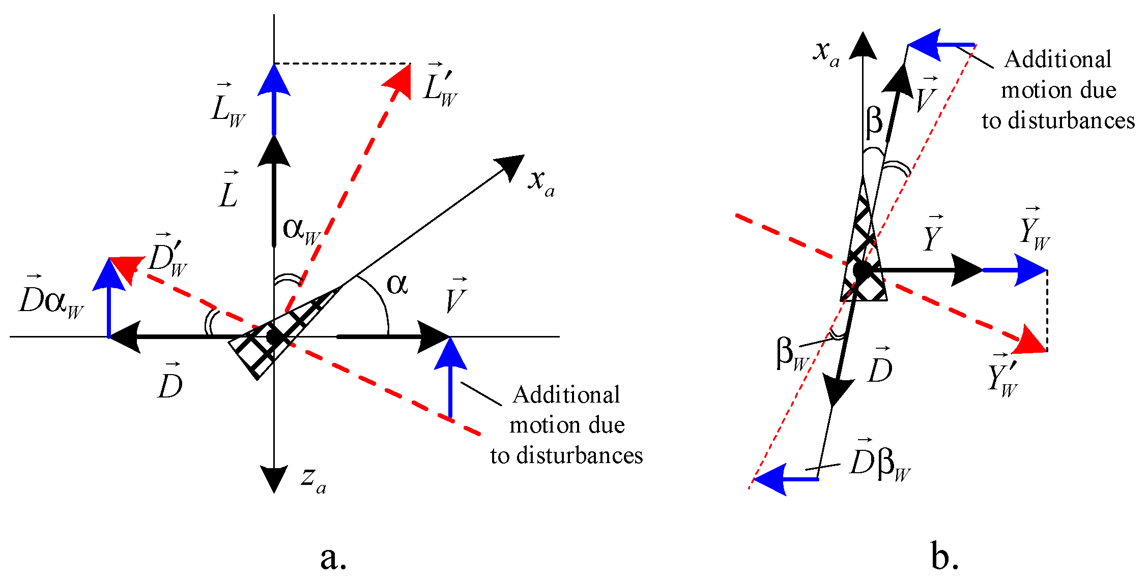
• Considering both the airwake and the wind type disturbances. Unlike most studies dealing with automatic carrier landing affected only by the carrier airwake, in this paper, the aircraft dynamics additionally take into account the three most important wind type disturbances, i.e., the wind shears, the wind gusts, and the atmospheric turbulences. Since the aircraft attack and sideslip angles are influenced both by the airwake and the wind type disturbances, the new dynamics reflect better the motion of the airplane.
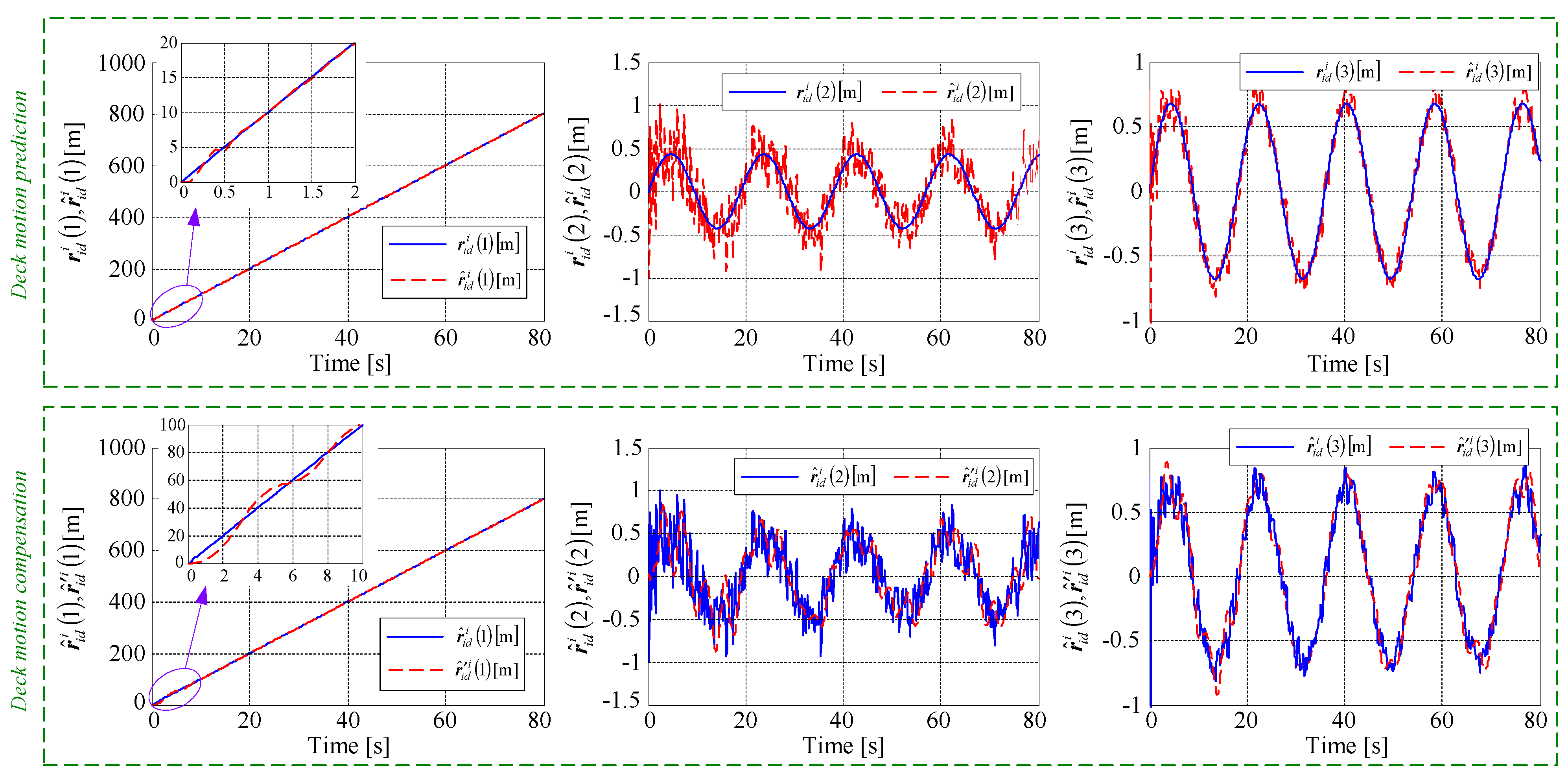
• Treating separately the prediction and the compensation problems via two independent blocks: (1) a block for the prediction of the deck motion and (2) a block for the compensation of the deck motion. The compensation of the deck motion is achieved by using the signal provided by the deck motion prediction block. This way, the aircraft can correct the position of the ideal touchdown point by using fewer signals from the ship, while the landing accuracy is improved by considering both the airplane-ship relative landing geometry and the configuration of the landing spot on the carrier. Compared to the existing literature, the prediction of the deck motion is achieved here with a recursive-least squares algorithm-based filter, while a tracking differentiator-based deck motion compensation block (TD-DMC) is used to solve the deck motion compensation problem. The TD-DMC blocks have been used so far only for obtaining the imposed values of the aircraft altitude [3]; compared to the classical DMCs, TD-DMC has a simplified structure and an easier parameter tuning.
• Obtaining anovel6-DOFdynamicswithangleofattackcontrolledbythrust. Considering the three wind type disturbances, we mathematically deduced the expressions of the new resultant disturbance type terms, and we included them in the 6-DOF dynamics of the airplane. Additionally, we considered a complete deck motion involving both maneuvering and seakeeping equations; a deterministic form is associated to the maneuvering part, while the seakeeping random motion refers to the motion affected by the wave excitation.
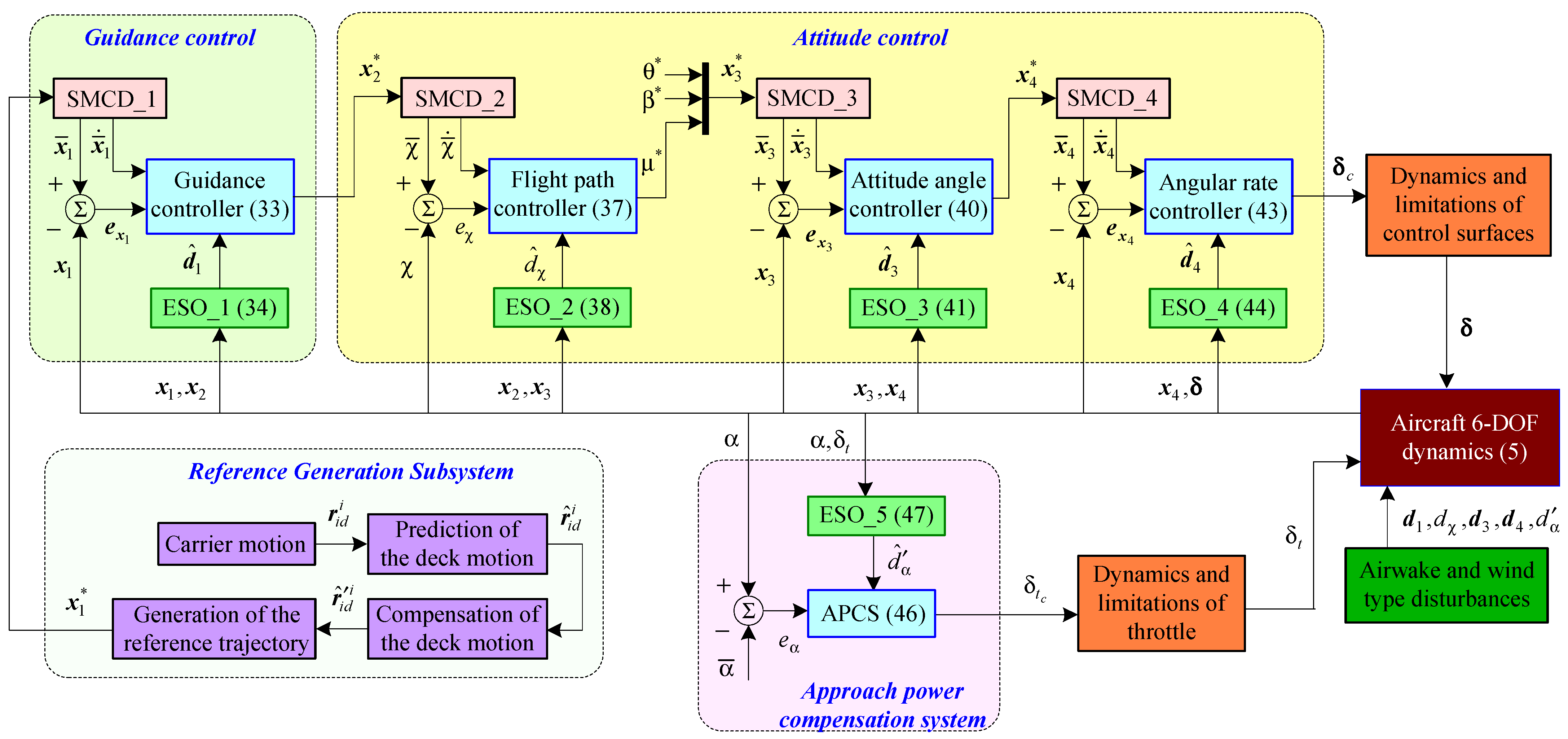
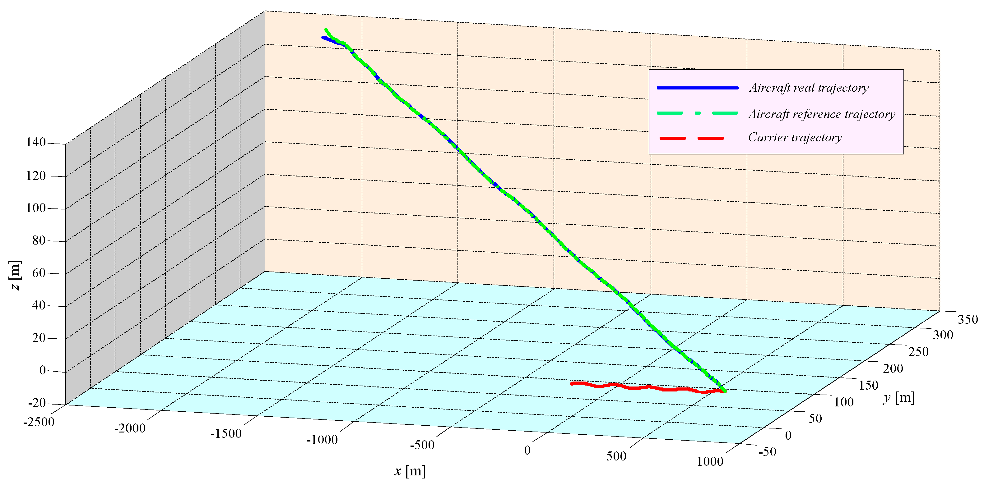
• Designing a control architecture mainly based on innovative combinations between sliding mode-based command differentiators, extended state observers, and backstepping-based controllers. Considering the influence of deck motion, airwake, and wind type disturbances, our novel ACLS has a classical configuration consisting of five control loops, i.e., guidance control, flight path angle control, control of the attitude angles, control of the angular rates, and approach power compensation subsystem. In four of the five loops, the sliding mode-based command differentiators are used to compute the virtual commands and their derivatives; then, five controllers are designed to track the generated commands. The novel ACLS is characterized by trajectory tracking capability, as well as excellent adaptability to the unexpected and even sudden changes in the state of the sea.
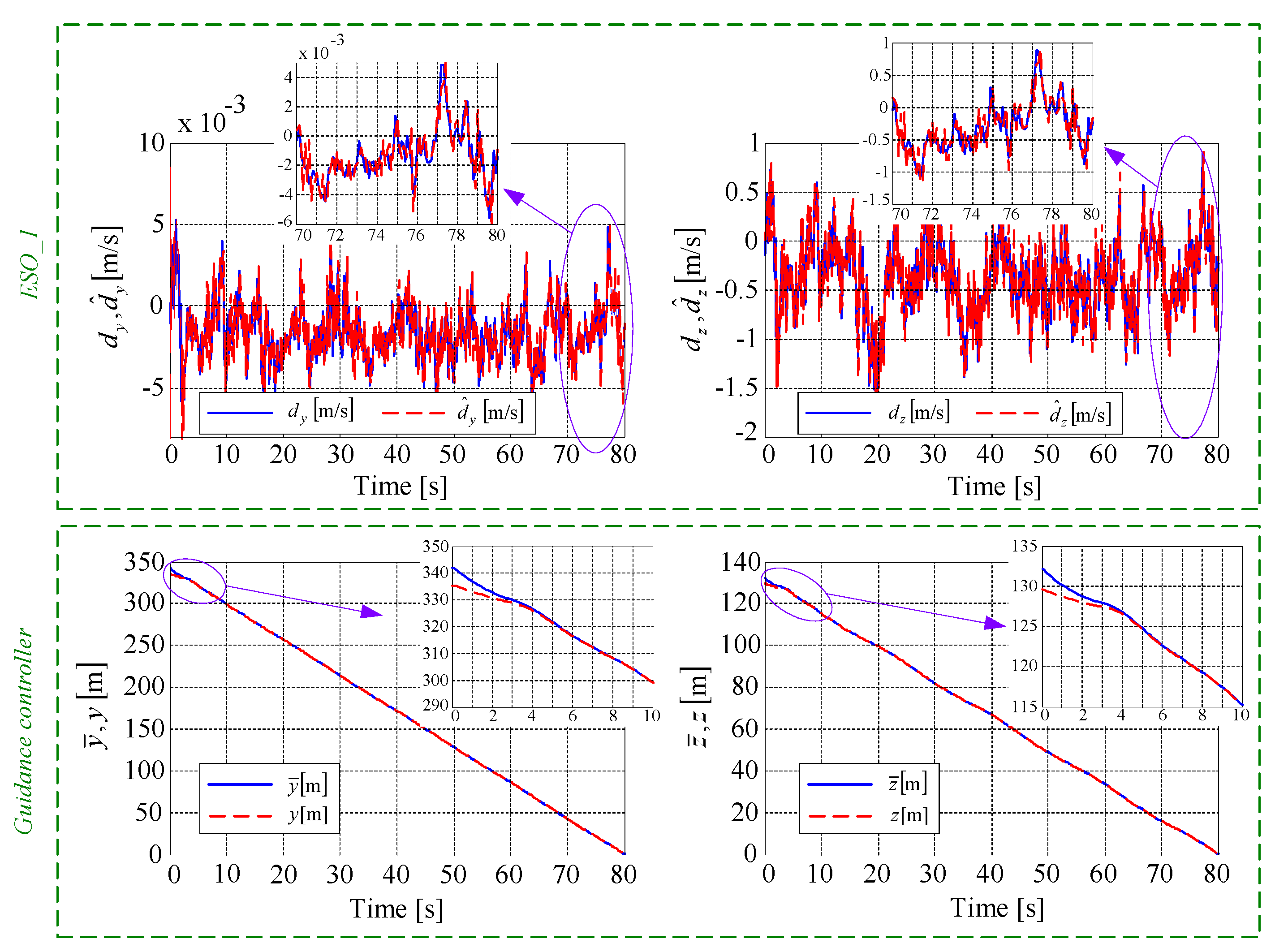
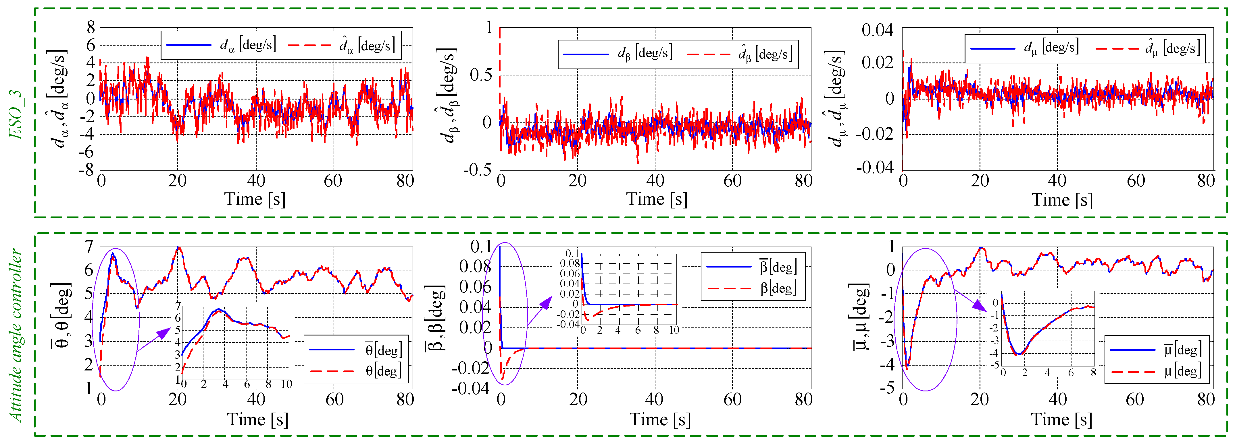
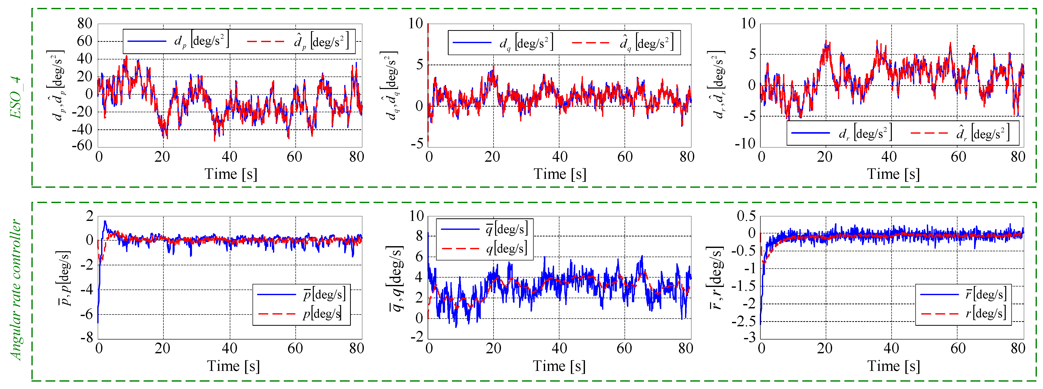
• Enhancing the robustness of the controllers via extended state observers. The disturbances depending on the airwake, the wind shears, the atmospheric turbulences, and the wind gusts are successfully estimated by using ESOs and then suppressed by means of the backstepping-based controllers.

The rest of the present work is organized as follows: the aircraft dynamics, the models of the airwake, the model of the wind type disturbances, as well as the mathematical expressions of the external disturbances are established in the next section. In Section 3, we deduce the deck motion dynamics, and we design the two blocks for the deck motion prediction and compensation. Section 4 deals with the deduction of the aircraft reference trajectory, the design of the SMCDs and ESOs, the design of the controllers, and the stability analysis. The fifth section includes both the software validation of the novel ACLS and the analysis of the obtained results. Finally, the sixth section of this work concludes the study and formulates some research directions for future research.

2. Aircraft Dynamics during Landing

The classical carrier landing involves three phases: final approach, glideslope, and touchdown. In the first two phases, the aircraft descends to a certain point (called “marchall” point) and then continues charging on a linear path to the point of contact with the runway. During the touchdown phase, the aircraft places the landing gear on the ship deck and brakes; this last stage is also carried out by means of a hook and four cables transversely positioned on the deck [31]. The glideslope is characterized by a constant speed and a slope angle $\left({\mathsf{\gamma }}_s\right)$ of −2.5 ÷ −3.5 deg, the trajectory being linear; the vertical speed at touchdown should be approximately 3–4 m/s. Several automatic control subsystems are used to control the aircraft trajectory. Some of these subsystems control the aircraft deviation in vertical plane relative to the desired downward trajectory by means of the elevator, while other subsystems control the deviation in lateral-directional plane relative to the desired trajectory via the deflections of rudder and ailerons; finally, the third category of subsystems control the speed and the attack angle by changing the engine operating mode.

2.1. Aircraft Model

The aircraft considered in this paper is the SIAI Marchetti S211 aircraft—a military training airplane produced by the Italian corporation SIAI-Marchetti since 1981; its geometry and aerodynamic data are reported in [32]. The airplane is equipped with a JTI5D-48 engine providing traction of 11.12 kN (25,000 lbs), maximum speed of 414 knots, and has a specific consumption of 0.57 lb/h. The control inputs of the airplane include the deflections of the elevator, rudder, ailerons, as well as the throttle command. The 6-DOF model of the airplane has been obtained by using the following reference frames: (1) $O_i{x}_i{y}_i{z}_i$—the inertial reference frame (North, East, and vertically down axes); (2) $O_a{x}_a{y}_a{z}_a$—the aircraft body-fixed reference frame ($O_a$—aircraft center of gravity, $O_a{x}_a$—longitudinal axis, $O_a{y}_a$—right plane-oriented axis, $O_a{z}_a$—vertical down axis); (3) $O_p{x}_p{y}_p{z}_p$—the ship body-fixed reference frame ($O_p$—ship center of gravity, $O_p{x}_p$—longitudinal axis of the carrier, $O_p{y}_p$—transversal axis of the carrier aircraft, $O_p{z}_p$—vertical axis oriented downward); (4) $O_d{x}_d{y}_d{z}_d$—the deck body-fixed reference frame ($O_d$—the desired touchdown point on the runway, $O_d{x}_d$—axis oriented parallel to the runway centerline, $O_d{z}_d$—vertical axis parallel to $O_p{z}_p$—axis, $O_d{y}_d$—axis perpendicular to the plane $O_d{x}_d{z}_d$). The four corresponding reference frames are depicted in Figure 1.

Assumption 1.

The aircraft is considered a rigid body, being symmetrical relative to the vertical plane $O_a{x}_a{z}_a\hspace{0.17em}$; its dynamics are described by bounded variables.

Assumption 2.

The motion information of the ship (i.e., position, linear velocities, angular rates, etc.) is measured and sent to the aircraft with very good accuracy. Moreover, the velocity of the aircraft is supposed to be higher than the speed of the ship, the aircraft being able to catch up to the target motion.

With proper transformations, the aircraft dynamics are described by the equations from [32], enriched in this paper with disturbance type terms whose expressions will be deduced in Section 2.3:

$$\left\{\begin{array}{l}\dot{V}=-g\sin \mathsf{\gamma }+\frac{T_{\max }{\mathsf{\delta }}_t\cos \mathsf{\alpha }\cos \mathsf{\beta }-D}{m}+d_V\hspace{0.17em},\\ \dot{\mathsf{\chi }}=\frac{1}{mV\cos \mathsf{\gamma }}\hspace{0.17em}\left[-Y\cos \mathsf{\mu }+L\sin \mathsf{\mu }+T_{\max }{\mathsf{\delta }}_t\hspace{0.17em}\left(\sin \mathsf{\alpha }\sin \mathsf{\mu }-\cos \mathsf{\alpha }\sin \mathsf{\beta }\cos \mathsf{\mu }\right)\right]+d_{\mathsf{\chi }},\\ \dot{\mathsf{\gamma }}=\frac{1}{mV}\hspace{0.17em}\left[-mg\cos \mathsf{\gamma }+Y\sin \mathsf{\mu }+L\cos \mathsf{\mu }+T_{\max }{\mathsf{\delta }}_t\hspace{0.17em}\left(\cos \mathsf{\alpha }\sin \mathsf{\beta }\sin \mathsf{\mu }+\sin \mathsf{\alpha }\cos \mathsf{\mu }\right)\right]+d_{\mathsf{\gamma }},\end{array}\right.$$

(1)

$$\left\{\begin{array}{l}\dot{\mathsf{\mu }}=\left(\sin \mathsf{\gamma }+\cos \mathsf{\gamma }\sin \mathsf{\mu }\tan \mathsf{\beta }\right)\hspace{0.17em}\hspace{0.17em}\dot{\mathsf{\chi }}+\cos \mathsf{\mu }\tan \mathsf{\beta }\hspace{0.17em}\hspace{0.17em}\dot{\mathsf{\gamma }}+\frac{\left(p\cos \mathsf{\alpha }+r\sin \mathsf{\alpha }\right)}{\cos \mathsf{\beta }}+d_{\mathsf{\mu }}\hspace{0.17em},\\ \dot{\mathsf{\alpha }}=-\frac{\cos \mathsf{\gamma }\sin \mathsf{\mu }}{\cos \mathsf{\beta }}\hspace{0.17em}\hspace{0.17em}\dot{\mathsf{\chi }}-\frac{\cos \mathsf{\mu }}{\cos \mathsf{\beta }}\hspace{0.17em}\hspace{0.17em}\dot{\mathsf{\gamma }}-p\cos \mathsf{\alpha }\tan \mathsf{\beta }+q-r\sin \mathsf{\alpha }\tan \mathsf{\beta }+d_{\mathsf{\alpha }}\hspace{0.17em},\\ \dot{\mathsf{\beta }}=\dot{\mathsf{\chi }}\hspace{0.17em}\cos \mathsf{\gamma }\cos \mathsf{\mu }-\dot{\mathsf{\gamma }}\hspace{0.17em}\sin \mathsf{\mu }+p\sin \mathsf{\alpha }-r\cos \mathsf{\alpha }+d_{\mathsf{\beta }}\hspace{0.17em},\end{array}\right.$$

(2)

$$\left\{\begin{array}{l}\dot{p}=I_{1}qr+I_{2}pq+I_3{M}_l+I_4{M}_n+d_p\hspace{0.17em},\\ \dot{q}=I_{5}pr+I_6\left(r^2-p^2\right)+I_7{M}_m+d_q\hspace{0.17em},\\ \dot{r}=-I_{2}qr+I_{8}pq+I_4{M}_l+I_9{M}_n+d_r\hspace{0.17em},\end{array}\right.$$

(3)

$$\dot{x}=V\cos \mathsf{\gamma }\cos \mathsf{\chi }+d_x,\hspace{0.17em}\hspace{0.17em}\dot{y}=V\cos \mathsf{\gamma }\sin \mathsf{\chi }+d_y,\hspace{0.17em}\hspace{0.17em}\dot{z}=-V\sin \mathsf{\gamma }+d_z\hspace{0.17em},$$

(4)

where $x,\hspace{0.17em}y,\hspace{0.17em}z$ are the aircraft position coordinates in inertial reference frame; V is the airplane speed; $\mathsf{\gamma }$ is the slope angle of the airplane trajectory; $\mathsf{\chi }$ is the heading angle; $T_{\max }$ is the maximum values of the thrust force; $\mathsf{\alpha },\hspace{0.17em}\mathsf{\beta },\hspace{0.17em}\mathsf{\mu }$ denote the attack angle, the sideslip angle, and the bank angle; ${\mathsf{\delta }}_t\in \left[0,\hspace{0.17em}1\right]$ is the throttle command; $D,\hspace{0.17em}L,\hspace{0.17em}Y$ are the drag, the lift, and the lateral forces (their expressions are given in Section 2.3); $p,\hspace{0.17em}q,\hspace{0.17em}r$ are the roll, pitch, and yaw angular rates; $I_k,\hspace{0.17em}k=\overline{1,\hspace{0.17em}9}\hspace{0.17em},$ are functions (given in Appendix A and Appendix B) of the axial inertia moments $\left(I_x,\hspace{0.17em}{I}_y,\hspace{0.17em}{I}_z\right)$ and the planar inertia moment $\left(I_{xz}\right)$, while $M_l,\hspace{0.17em}{M}_m,\hspace{0.17em}{M}_n$ are the roll, pitch, and yaw aerodynamic moments (also presented in Appendix A and Appendix B).

Before the design of the ACLS, the mathematical description of the aircraft is rewritten into an affine form; for this, we proceed to some notations: ${\mathit{x}}_1={\left[\begin{array}{cc}y& z\end{array}\right]}^{\hspace{0.17em}\mathrm{T}},\hspace{0.17em}{\mathit{x}}_2={\left[\begin{array}{cc}\mathsf{\chi }& \mathsf{\gamma }\end{array}\right]}^{\hspace{0.17em}\mathrm{T}},\hspace{0.17em}{\mathit{x}}_3={\left[\begin{array}{ccc}\mathsf{\theta }& \mathsf{\beta }& \mathsf{\mu }\end{array}\right]}^{\hspace{0.17em}\mathrm{T}},\hspace{0.17em}$${\mathit{x}}_4={\left[\begin{array}{ccc}p& q& r\end{array}\right]}^{\hspace{0.17em}\mathrm{T}},\hspace{0.17em}\mathsf{\delta }={\left[\begin{array}{ccc}{\mathsf{\delta }}_a& {\mathsf{\delta }}_e& {\mathsf{\delta }}_r\end{array}\right]}^{\hspace{0.17em}\mathrm{T}},\hspace{0.17em}{\mathit{d}}_1={\left[\begin{array}{cc}{d}_y& d_z\end{array}\right]}^{\hspace{0.17em}\mathrm{T}},\hspace{0.17em}{\mathit{d}}_3={\left[\begin{array}{ccc}{d}_{\mathsf{\alpha }}& d_{\mathsf{\beta }}& d_{\mathsf{\mu }}\end{array}\right]}^{\hspace{0.17em}\mathrm{T}},$${\mathit{d}}_4={\left[\begin{array}{ccc}{d}_p& d_q& d_r\end{array}\right]}^{\hspace{0.17em}\mathrm{T}}.$ According to the issues presented above, we rewrite (1)–(4) into an affine form as follows:

$$\left\{\begin{array}{l}{\dot{\mathit{x}}}_1={\mathit{f}}_1\left({\mathit{x}}_2\hspace{0.17em},\hspace{0.17em}V\right)+{\mathit{b}}_1\left(V\right)\hspace{0.17em}{\mathit{x}}_2+{\mathit{d}}_1\hspace{0.17em},\\ {\dot{\mathit{x}}}_2\left(1\right)=f_2\left({\mathit{x}}_2\hspace{0.17em},\hspace{0.17em}{\mathit{x}}_3\hspace{0.17em},\hspace{0.17em}V\right)+b_2\left({\mathit{x}}_2\hspace{0.17em},\hspace{0.17em}V\right)\hspace{0.17em}{\mathit{x}}_3\left(3\right)+d_{\mathsf{\chi }}\hspace{0.17em},\\ {\dot{\mathit{x}}}_3={\mathit{f}}_3\left({\dot{\mathit{x}}}_2\hspace{0.17em},\hspace{0.17em}{\mathit{x}}_2\hspace{0.17em},\hspace{0.17em}{\mathit{x}}_3\right)+{\mathit{b}}_3\left({\mathit{x}}_2\hspace{0.17em},\hspace{0.17em}{\mathit{x}}_3\right)\hspace{0.17em}{\mathit{x}}_4+{\mathit{d}}_3\hspace{0.17em},\\ {\dot{\mathit{x}}}_4={\mathit{f}}_4\left({\mathit{x}}_3\hspace{0.17em},\hspace{0.17em}{\mathit{x}}_4\hspace{0.17em},\hspace{0.17em}V\right)+{\mathit{b}}_4\left(V\right)\hspace{0.17em}\mathsf{\delta }+{\mathit{d}}_4\hspace{0.17em},\\ \dot{\mathsf{\alpha }}=f_{\mathsf{\alpha }}\left({\mathit{x}}_2\hspace{0.17em},\hspace{0.17em}{\mathit{x}}_4\hspace{0.17em},\hspace{0.17em}V\right)+b_{\mathsf{\alpha }}\left(V\right)\hspace{0.17em}{\mathsf{\delta }}_t+{d^{\prime }}_{\mathsf{\alpha }}\hspace{0.17em},\end{array}\right.$$

(5)

with ${\mathit{x}}_2\left(1\right)=\mathsf{\chi },\hspace{0.17em}\hspace{0.17em}{\mathit{x}}_3\left(3\right)=\mathsf{\mu }\hspace{0.17em}$; the explicit expressions of ${\mathit{f}}_i,\hspace{0.17em}{\mathit{b}}_i\hspace{0.17em}\left(i=1,\hspace{0.17em}2,\hspace{0.17em}3,\hspace{0.17em}4,\hspace{0.17em}\mathsf{\alpha }\right)\hspace{0.17em}$, and disturbance ${d^{\prime }}_{\mathsf{\alpha }}$ are provided in Appendix A and Appendix B, while the expressions of the disturbance type terms are deduced in this section.

Assumption 3.

The disturbances included in dynamics from Equation(5), namely ${\mathit{d}}_1\hspace{0.17em},\hspace{0.17em}{d}_{\mathsf{\chi }}\hspace{0.17em},\hspace{0.17em}{\mathit{d}}_3\hspace{0.17em},\hspace{0.17em}{\mathit{d}}_4\hspace{0.17em},\hspace{0.17em}{d^{\prime }}_{\mathsf{\alpha }}\hspace{0.17em}$, are bounded by unknown constants, i.e., $‖{\mathit{d}}_i‖\le {\overline{d}}_i\hspace{0.17em}$, with $i=1,\hspace{0.17em}\mathsf{\chi },\hspace{0.17em}3,\hspace{0.17em}4,\hspace{0.17em}\mathsf{\alpha }\hspace{0.17em}$.

Remark 1.

The 6-DOF affine dynamics from Equation (5) contain novelty; compared to the nonlinear dynamics deduced in [20,21,22,33], where some disturbances have been not considered, all the equations from the model shown in Equation (5) contain external disturbances, thus making the aircraft dynamics closer to the real case.

Remark 2.

The affine dynamics from some studies (e.g., [34]) were obtained by independently controlling the aircraft speed via the thrust force, but these results cannot be directly used in the design of the automatic carrier landing controller. Therefore, we obtained novel nonlinear dynamics, which consider the attack angle not the speed controlled by thrust.

Remark 3.

The control of the aircraft during landing is obtained by going through the three control surfaces (ailerons, elevator, and rudder) and also by adjusting the thrust. The dynamics of actuators relating the control inputs ${\mathsf{\delta }}_a\hspace{0.17em},\hspace{0.17em}{\mathsf{\delta }}_e\hspace{0.17em},\hspace{0.17em}{\mathsf{\delta }}_r\hspace{0.17em},\hspace{0.17em}{\mathsf{\delta }}_t$and the outputs of the controllers $\left({\mathsf{\delta }}_{a_c}\hspace{0.17em},\hspace{0.17em}{\mathsf{\delta }}_{e_c}\hspace{0.17em},\hspace{0.17em}{\mathsf{\delta }}_{r_c}\hspace{0.17em},\hspace{0.17em}{\mathsf{\delta }}_{t_c}\right)$ are: ${\dot{\mathsf{\delta }}}_j=-\frac{1}{{\mathsf{\tau }}_j}\hspace{0.17em}{\mathsf{\delta }}_j+\frac{1}{{\mathsf{\tau }}_j}\hspace{0.17em}{\mathsf{\delta }}_{j_c}$, with j = a, e, r, t; ${\mathsf{\tau }}_j$ representing the time constants of the actuators and of the engine, respectively [32]. For SIAI Marchetti S211 airplane, the constants are: ${\mathsf{\tau }}_e={\mathsf{\tau }}_a={\mathsf{\tau }}_r=0.0495,\hspace{0.17em}{\mathsf{\tau }}_t=1$. The rate limits for the elevator, ailerons, and rudder are: [−60 deg/s; 60 deg/s], [−80 deg/s; 80 deg/s], and [−120 deg/s; 120 deg/s], respectively. The position limits are [−25 deg; 25 deg], [−21.5 deg; 21.5 deg], and [−30 deg; 30 deg], respectively.

2.2. Models of Airwake and Wind Type Disturbances

The accuracy of landing is mainly affected by the external disturbances (airwake and wind type disturbances). The airwake is strong behind the aircraft carrier and, therefore, the airplane may be blown away from the reference trajectory in the last part of the carrier landing process. On the contrary, the wind is a disturbance, which alters the aircraft attitude and velocity during all the three phases of landing. Unlike most studies dealing with the automatic carrier landing, where only the airwake was considered, the present paper considers both the airwake and the wind type disturbances (wind shears, atmospheric turbulences, wind gusts) in the dynamics of the airplane.

According to [3], the airwake type turbulence consists of four parts: free-air turbulence, constant and random carrier-wake turbulences created by the waves that are produced by the aircraft carrier, and turbulence induced by the periodic motion of the carrier. Subsequently, the models of airwake type turbulences are described below.

Free-air turbulences do not depend on the aircraft position, being calculated by passing a white noise through a filter; the transfer functions associated to the three components of the free-air turbulence are [35]:

$$H_{u_1}\left(\mathrm{s}\right)=\frac{u_1\left(\mathrm{s}\right)}{\mathsf{\eta }\left(\mathrm{s}\right)}=\sqrt{\frac{200}{V}}\frac{1}{1+\frac{100\mathrm{s}}{V}},\hspace{0.17em}{H}_{v_1}\left(\mathrm{s}\right)=\frac{v_1\left(\mathrm{s}\right)}{\mathsf{\eta }\left(\mathrm{s}\right)}=\sqrt{\frac{5900}{V}}\frac{1+\frac{400\mathrm{s}}{V}}{1+\frac{700\mathrm{s}}{3V}+\frac{4\cdot {10}^4}{3V^2}},\hspace{0.17em}{H}_{w_1}\left(\mathrm{s}\right)=\frac{w_1\left(\mathrm{s}\right)}{\mathsf{\eta }\left(\mathrm{s}\right)}=\sqrt{\frac{71.6}{V}}\frac{1}{1+\frac{100\mathrm{s}}{V}}\hspace{0.17em},$$

(6)

where $u_1,\hspace{0.17em}{v}_1,\hspace{0.17em}{w}_1$ are the components (speeds) of free-air turbulence along the longitudinal, lateral, and vertical axes; $V$ is the aircraft speed, while $\mathsf{\eta }$ is a band-limited white noise.

The constant carrier-wake turbulences are mainly produced by the waves created by the ship and the air flowing on the back of the aircraft carrier. The lateral component of this turbulence is negligible $\left(v_2=0\right)\hspace{0.17em}$, while the horizontal $\left(u_2\right)$ and the vertical $\left(w_2\right)$ components depend on the distance between the ship center of mass and the aircraft center of mass. Using the graphic from [35], we made some approximations for the velocities $u_2$ and $w_2$ in relation to the distance between the airplane and the desired touchdown point ($d_c$ [ft]):

$$u_2\cong \left\{\begin{array}{l}0\hspace{0.17em}\hspace{0.17em},\hspace{0.17em}\hspace{0.17em}\hspace{0.17em}{d}_c\in \left[-3000\hspace{0.17em},\hspace{0.17em}-1800\right)\\ 0.025\hspace{0.17em}{V}_{w/d}\hspace{0.17em}\hspace{0.17em},\hspace{0.17em}\hspace{0.17em}\hspace{0.17em}{d}_c\in \left[-1800\hspace{0.17em},\hspace{0.17em}-1400\right)\\ 0.04\hspace{0.17em}{V}_{w/d}\hspace{0.17em}\hspace{0.17em},\hspace{0.17em}\hspace{0.17em}\hspace{0.17em}{d}_c\in \left[-1400\hspace{0.17em},\hspace{0.17em}-1000\right)\\ 0.1\hspace{0.17em}{V}_{w/d}\hspace{0.17em}\hspace{0.17em},\hspace{0.17em}\hspace{0.17em}\hspace{0.17em}{d}_c\in \left[-1000\hspace{0.17em},\hspace{0.17em}-400\right)\\ 0.05\hspace{0.17em}{V}_{w/d}\hspace{0.17em}\hspace{0.17em},\hspace{0.17em}\hspace{0.17em}\hspace{0.17em}{d}_c\in \left[-400\hspace{0.17em},\hspace{0.17em}0\right]\end{array}\right.\hspace{0.17em},\hspace{0.17em}\hspace{0.17em}\hspace{0.17em}{w}_2\cong \left\{\begin{array}{l}0\hspace{0.17em}\hspace{0.17em},\hspace{0.17em}\hspace{0.17em}\hspace{0.17em}{d}_c\in \left[-3000\hspace{0.17em},\hspace{0.17em}-2600\right)\\ -0.06\hspace{0.17em}{V}_{w/d}\hspace{0.17em}\hspace{0.17em},\hspace{0.17em}\hspace{0.17em}\hspace{0.17em}{d}_c\in \left[-2600\hspace{0.17em},\hspace{0.17em}-2200\right)\\ -0.05\hspace{0.17em}{V}_{w/d}\hspace{0.17em}\hspace{0.17em},\hspace{0.17em}\hspace{0.17em}\hspace{0.17em}{d}_c\in \left[-2200\hspace{0.17em},\hspace{0.17em}-1500\right)\\ -0.015\hspace{0.17em}{V}_{w/d}\hspace{0.17em}\hspace{0.17em},\hspace{0.17em}\hspace{0.17em}\hspace{0.17em}{d}_c\in \left[-1500\hspace{0.17em},\hspace{0.17em}-750\right)\\ 0.01\hspace{0.17em}{V}_{w/d}\hspace{0.17em}\hspace{0.17em},\hspace{0.17em}\hspace{0.17em}\hspace{0.17em}{d}_c\in \left[-750\hspace{0.17em},\hspace{0.17em}0\right]\end{array}\right.\hspace{0.17em}\hspace{0.17em},$$

(7)

where $\hspace{0.17em}{V}_{w/d}\hspace{0.17em}\left[\mathrm{ft}/\mathrm{s}\right]$ is the wind speed over the deck.

The random carrier-wake turbulences can be generated by filtering white noises and depend on the deck wind $\hspace{0.17em}{V}_{w/d}\hspace{0.17em}\left[\mathrm{ft}/\mathrm{s}\right]$ and the distance between the aircraft and the touchdown point. The transfer functions associated to the horizontal and the vertical components ($u_3$ and $w_3$) are [2]:

$$H_{u_3}\left(\mathrm{s}\right)=\frac{u_3\left(\mathrm{s}\right)}{\widehat{\mathsf{\eta }}\left(\mathrm{s}\right)}=\frac{\mathsf{\sigma }\left(d_c\right)\sqrt{2\mathsf{\tau }\left(d_c\right)}}{\mathsf{\tau }\left(d_c\right)\mathrm{s}+1},\hspace{0.17em}\hspace{0.17em}{H}_{v_3}\left(\mathrm{s}\right)=\frac{v_3\left(\mathrm{s}\right)}{\widehat{\mathsf{\eta }}\left(\mathrm{s}\right)}=\frac{0.035V_{w/d}\sqrt{6.66}}{3.33\mathrm{s}+1},\hspace{0.17em}\hspace{0.17em}{H}_{w_3}\left(\mathrm{s}\right)=\frac{w_3\left(\mathrm{s}\right)}{\widehat{\mathsf{\eta }}\left(\mathrm{s}\right)}=\frac{0.035V_{w/d}\sqrt{6.66}}{3.33\mathrm{s}+1}\hspace{0.17em},$$

(8)

where $\mathsf{\sigma }\left(d_c\right)$ and the time constant $\mathsf{\tau }\left(d_c\right)$ are computed in [35] as percentage of the speed $\hspace{0.17em}{V}_{w/d}$ depending on the distance between aircraft and its ideal touchdown point:

$$\mathsf{\sigma }\left(d_c\right)\cong \left\{\begin{array}{l}0.01\hspace{0.17em}{V}_{w/d}\hspace{0.17em}\hspace{0.17em},\hspace{0.17em}\hspace{0.17em}\hspace{0.17em}{d}_c\in \left[-3000\hspace{0.17em},\hspace{0.17em}-2000\right)\\ 0.02\hspace{0.17em}{V}_{w/d}\hspace{0.17em}\hspace{0.17em},\hspace{0.17em}\hspace{0.17em}\hspace{0.17em}{d}_c\in \left[-2000\hspace{0.17em},\hspace{0.17em}-1500\right)\\ 0.04\hspace{0.17em}{V}_{w/d}\hspace{0.17em}\hspace{0.17em},\hspace{0.17em}\hspace{0.17em}\hspace{0.17em}{d}_c\in \left[-1500\hspace{0.17em},\hspace{0.17em}-1000\right)\\ 0.03\hspace{0.17em}{V}_{w/d}\hspace{0.17em}\hspace{0.17em},\hspace{0.17em}\hspace{0.17em}\hspace{0.17em}{d}_c\in \left[-1000\hspace{0.17em},\hspace{0.17em}-500\right)\\ 0.05\hspace{0.17em}{V}_{w/d}\hspace{0.17em}\hspace{0.17em},\hspace{0.17em}\hspace{0.17em}\hspace{0.17em}{d}_c\in \left[-500\hspace{0.17em},\hspace{0.17em}0\right]\end{array}\right.\hspace{0.17em},\hspace{0.17em}\hspace{0.17em}\hspace{0.17em}\mathsf{\tau }\left(d_c\right)\cong \left\{\begin{array}{l}1\hspace{0.17em}\sec \hspace{0.17em}\hspace{0.17em},\hspace{0.17em}\hspace{0.17em}\hspace{0.17em}{d}_c\in \left[-3000\hspace{0.17em},\hspace{0.17em}-2000\right)\\ 1\hspace{0.17em}\sec \hspace{0.17em}\hspace{0.17em},\hspace{0.17em}\hspace{0.17em}\hspace{0.17em}{d}_c\in \left[-2000\hspace{0.17em},\hspace{0.17em}-1500\right)\\ 1.1\hspace{0.17em}\sec \hspace{0.17em}\hspace{0.17em},\hspace{0.17em}\hspace{0.17em}\hspace{0.17em}{d}_c\in \left[-1500\hspace{0.17em},\hspace{0.17em}-1000\right)\\ 0.4\hspace{0.17em}\sec \hspace{0.17em}\hspace{0.17em},\hspace{0.17em}\hspace{0.17em}\hspace{0.17em}{d}_c\in \left[-1000\hspace{0.17em},\hspace{0.17em}-500\right)\\ 0.4\hspace{0.17em}\sec \hspace{0.17em}\hspace{0.17em},\hspace{0.17em}\hspace{0.17em}\hspace{0.17em}{d}_c\in \left[-500\hspace{0.17em},\hspace{0.17em}0\right]\end{array}\right.\hspace{0.17em}\hspace{0.17em}.$$

(9)

In Equation (8), the white noise $\widehat{\mathsf{\eta }}$ is chosen as follows [36]: $\widehat{\mathsf{\eta }}=\mathsf{\eta }\frac{j\mathsf{\omega }}{j\mathsf{\omega }+1}\hspace{0.17em}\sin \hspace{0.17em}\left(10\mathsf{\pi }t\right).$

The turbulence induced by the periodic motion of the aircraft carrier occurs because of the heave motion of the carrier; the lateral component has negligible values, while the horizontal and the vertical components depend on the wind speed on the deck, ship heave frequency $\left({\mathsf{\omega }}_p\right)\hspace{0.17em}$, pitch angle induced by the ship heave motion $\left({\mathsf{\theta }}_p\right)\hspace{0.17em}$, aircraft speed (V), and distance between the airplane and the desired touchdown point (d_c). The expressions for the horizontal and vertical components are [36]:

$$u_4={\mathsf{\theta }}_p{V}_{w/d}\hspace{0.17em}\left(2.22+0.009d_c\right)\hspace{0.17em}C,\hspace{0.17em}\hspace{0.17em}{w}_4={\mathsf{\theta }}_p{V}_{w/d}\hspace{0.17em}\left(4.98+0.0018d_c\right)\hspace{0.17em}C\hspace{0.17em},$$

(10)

where $C=\cos \hspace{0.17em}\left\{{\mathsf{\omega }}_p\left[t\hspace{0.17em}\left(1-\frac{V-V_{w/d}}{0.85V_{w/d}}\right)+\frac{d_c}{0.85V_{w/d}}\right]+P\right\}\hspace{0.17em},$ with $P$—random phase. One should mention that $u_4=0$ if $d_c>2236\hspace{0.17em}\mathrm{ft}$ and $w_4=0$ if $d_c>2536\hspace{0.17em}\mathrm{ft}.$ In Equation (10), the time t can be computed by considering constant values for the velocities of the airplane (V = 37 m/s $\cong$ 121.36 ft/s) and of the ship (V_p = 10 m/s $\cong$ 32.8 ft/s); one obtains: $t\cong \frac{d_c}{V-V_p}\cong \frac{d_c\hspace{0.17em}\left[\mathrm{ft}\right]}{88.56\hspace{0.17em}\left[\mathrm{ft}/\mathrm{s}\right]}\hspace{0.17em}.$ We borrowed from [35] the following values: ${\mathsf{\theta }}_p=0.018\hspace{0.17em}\mathrm{rad},\hspace{0.17em}{\mathsf{\omega }}_p=0.62\hspace{0.17em}\mathrm{rad}/\mathrm{s},\hspace{0.17em}{V}_{w/d}=9.84\hspace{0.17em}\mathrm{ft}/\mathrm{s},\hspace{0.17em}P=\mathsf{\pi }/4.$

Although the airwake has a greater influence on landing than a wind type disturbance, the latter should be also considered in the aircraft dynamics. Thus, the equations of the atmospheric turbulences, wind shears, and gusts are included into the airplane dynamics. One defines three vectors: ${\mathit{W}}_5={\left[\begin{array}{ccc}{u}_5& v_5& w_5\end{array}\right]}^{\hspace{0.17em}\mathrm{T}}$—the velocity vector associated to the wind shears, ${\mathit{W}}_6={\left[\begin{array}{ccc}{u}_6& v_6& w_6\end{array}\right]}^{\hspace{0.17em}\mathrm{T}}$—the velocity vector associated to the Dryden atmospheric turbulences, and ${\mathit{W}}_7={\left[\begin{array}{ccc}{u}_7& v_7& w_7\end{array}\right]}^{\hspace{0.17em}\mathrm{T}}$—the wind gust velocity vector.

The wind shears occur from a variety of geographical or atmospheric factors. The mean wind shear has the magnitude [37]: ${\mathit{W}}_5=W_{20}\frac{\ln \hspace{0.17em}\left(H/z_0\right)}{\ln \hspace{0.17em}\left(6.096/z_0\right)},\hspace{0.17em}\hspace{0.17em}1\hspace{0.17em}\mathrm{m}<H<\hspace{0.17em}300\hspace{0.17em}\mathrm{m}\hspace{0.17em},$ with $W_{20}$—the wind speed at 20 ft, H—the flight altitude, while $z_0$ depends on the flight stage.

The atmospheric turbulences are stochastic processes defined by means of the velocity spectra. In the Dryden spectral model, the longitudinal, the lateral, and the vertical spectra functions are presented in MIL-HDBK-1797/1797B [38]:

$$H_u\left(\mathrm{s}\right)={\mathsf{\sigma }}_u\sqrt{\frac{2L_u}{\mathsf{\pi }V}}\hspace{0.17em}\frac{1}{1+\frac{L_u}{V}\mathrm{s}},\hspace{0.17em}{H}_v\left(\mathrm{s}\right)={\mathsf{\sigma }}_v\sqrt{\frac{2L_v}{\mathsf{\pi }V}}\hspace{0.17em}\frac{1+\frac{\sqrt{3}{L}_v}{V}\mathrm{s}}{{\left(1+\frac{L_v}{V}\mathrm{s}\right)}^2},\hspace{0.17em}{H}_w\left(\mathrm{s}\right)={\mathsf{\sigma }}_w\sqrt{\frac{2L_w}{\mathsf{\pi }V}}\hspace{0.17em}\frac{1+\frac{\sqrt{3}{L}_w}{V}\mathrm{s}}{{\left(1+\frac{L_w}{V}\mathrm{s}\right)}^2}\hspace{0.17em},$$

(11)

where $L_u,\hspace{0.17em}{L}_v,\hspace{0.17em}{L}_w$ represent the turbulence scale lengths, while ${\mathsf{\sigma }}_u,\hspace{0.17em}{\mathsf{\sigma }}_v,\hspace{0.17em}{\mathsf{\sigma }}_w$ are the intensities of the turbulence. At low altitude, $W_{20}$ is 15 knots for light turbulences, 30 knots for moderate turbulences, and 45 knots for severe turbulences; the scale lengths and the intensities are [39]: $L_u=\frac{H}{{\left(0.177+0.000832H\right)}^{1.2}},\hspace{0.17em}{L}_w=H,\hspace{0.17em}{\mathsf{\sigma }}_u=\frac{{\mathsf{\sigma }}_w}{{\left(0.177+0.000832H\right)}^{0.4}},\hspace{0.17em}{\mathsf{\sigma }}_w=0.1\cdot W_{20}.$

The wind gusts use the implementation of a standard “1-cos” function, being associated to the Military Specification MIL-F-8785C; their expression is [40]:

$${\mathit{W}}_7=\left\{\begin{array}{l}0\hspace{0.17em},\hspace{0.17em}\hspace{0.17em}\hspace{0.17em}\tilde{x}<0\hspace{0.17em},\\ \frac{W_m}{2}\hspace{0.17em}\left(1-\cos \hspace{0.17em}\frac{\mathsf{\pi }X}{d_m}\right)\hspace{0.17em},\hspace{0.17em}\hspace{0.17em}\hspace{0.17em}0\le \tilde{x}\le d_m\hspace{0.17em},\\ W_m\hspace{0.17em},\hspace{0.17em}\hspace{0.17em}\hspace{0.17em}\tilde{x}>d_m\hspace{0.17em},\end{array}\right.$$

(12)

where $\tilde{x}$ is the travelled distance, while $W_m$ and $d_m$ are the gust magnitude and length.

Considering both the airwake and the wind disturbances, we define the components of the resultant disturbance: $u_W={\displaystyle \sum _{j=1}^7{u}_j},\hspace{0.17em}\hspace{0.17em}{v}_W={\displaystyle \sum _{j=1}^7{v}_j},\hspace{0.17em}\hspace{0.17em}{w}_W={\displaystyle \sum _{j=1}^7{w}_j}\hspace{0.17em};$ index j is 1, 2, 3, 4 for airwake and 5, 6, 7 for the other three wind type disturbances.

2.3. Mathematical Expressions of the External Disturbances

The wind and the disturbances caused by waves lead to the modification of the aircraft attack and sideslip angles. Thus, supplementary dimensionless angles appear (measured in [rad]): ${\mathsf{\alpha }}_W=\frac{w_W}{V}$ and ${\mathsf{\beta }}_W=-\frac{v_W}{V}\hspace{0.17em}$; the influence of these supplementary angles on the aerodynamic forces acting in longitudinal and lateral-directional planes is graphically presented in Figure 2. The black color has been used to present the forces in the absence of the disturbances, while the blue color and the red color were employed to figure out the forces if the disturbances are taken into account.

The expressions of the drag (D), lift (L), and lateral force (Y) are [36]:

$$D=p_{d}S{C}_D=\frac{\mathsf{\rho }{V}^2}{2}S{C}_D,\hspace{0.17em}\hspace{0.17em}L=p_{d}S{C}_L=\frac{\mathsf{\rho }{V}^2}{2}S{C}_L,\hspace{0.17em}\hspace{0.17em}Y=p_{d}S{C}_Y=\frac{\mathsf{\rho }{V}^2}{2}S{C}_Y\hspace{0.17em},$$

(13)

where $p_d=\mathsf{\rho }{V}^2/2$ is the aircraft dynamic pressure, $S$ is the wing area, while the drag force coefficient (C_D), the lift force coefficient (C_L), and the lateral force coefficient (C_Y) are [41]:

$$\begin{array}{l}{C}_D=C_{D_0}+C_{D_{\mathsf{\alpha }}}\mathsf{\alpha }+\frac{\overline{c}}{2V}\hspace{0.17em}{C}_{D_q}q+C_{D_{{\mathsf{\delta }}_e}}{\mathsf{\delta }}_e,\hspace{0.17em}\hspace{0.17em}\\ C_L=C_{L_0}+C_{L_{\mathsf{\alpha }}}\mathsf{\alpha }+\frac{\overline{c}}{2V}{C}_{L_q}q+C_{L_{{\mathsf{\delta }}_e}}{\mathsf{\delta }}_e,\hspace{0.17em}\hspace{0.17em}\\ C_Y=C_{Y_0}+C_{Y_{\mathsf{\beta }}}\mathsf{\beta }+\frac{b}{2V}\left(C_{Y_p}p+C_{Y_r}r\right)+C_{Y_{{\mathsf{\delta }}_r}}{\mathsf{\delta }}_r+C_{Y_{{\mathsf{\delta }}_a}}{\mathsf{\delta }}_a\hspace{0.17em},\end{array}$$

(14)

with $b$—wing span, $\overline{c}$—aerodynamic mean chord, ${\mathsf{\delta }}_e$—elevator deflection, ${\mathsf{\delta }}_r$—rudder deflection, ${\mathsf{\delta }}_a$—deflection of ailerons, $C_{D_0},\hspace{0.17em}{C}_{D_{\mathsf{\alpha }}},\hspace{0.17em}{C}_{D_q},\hspace{0.17em}{C}_{L_0},\hspace{0.17em}{C}_{L_{\mathsf{\alpha }}},\hspace{0.17em}{C}_{L_q}$—longitudinal stability derivatives, $C_{Y_0},\hspace{0.17em}{C}_{Y_{\mathsf{\beta }}},\hspace{0.17em}{C}_{Y_p},\hspace{0.17em}{C}_{Y_r}$—lateral-directional stability derivatives, $C_{D_{{\mathsf{\delta }}_e}},\hspace{0.17em}{C}_{L_{{\mathsf{\delta }}_e}}$—longitudinal control derivatives, while $C_{Y_{{\mathsf{\delta }}_r}},\hspace{0.17em}{C}_{Y_{{\mathsf{\delta }}_a}}$—lateral-directional control derivatives.

According to Figure 2a, the new attack angle is $\mathsf{\alpha }+{\mathsf{\alpha }}_W$; therefore, the lift force coefficient becomes:

$${C^{\prime }}_L=C_{L_0}+C_{L_{\mathsf{\alpha }}}\left(\mathsf{\alpha }+{\mathsf{\alpha }}_W\right)+\frac{\overline{c}}{2V}{C}_{L_q}q+C_{L_{{\mathsf{\delta }}_e}}{\mathsf{\delta }}_e=C_L+C_{L_{\mathsf{\alpha }}}{\mathsf{\alpha }}_W,$$

(15)

while the lift force obtains the form: $L^{\prime }=\frac{\mathsf{\rho }{V}^2}{2}S\left(C_L+C_{L_{\mathsf{\alpha }}}{\mathsf{\alpha }}_W\right)=L+L_W\hspace{0.17em},$ where $L_W=\frac{\mathsf{\rho }{V}^2}{2}S{C}_{L_{\mathsf{\alpha }}}{\mathsf{\alpha }}_W$. Using these expressions and Figure 2a, the new expression of the lift force is deduced:

$${L^{\prime }}_W=\left(L+L_W+D{\mathsf{\alpha }}_W\right)\hspace{0.17em}\cos {\mathsf{\alpha }}_W\cong L+L_W+D{\mathsf{\alpha }}_W\hspace{0.17em}.$$

(16)

Similarly, improved expressions are obtained for the drag and the lateral forces:

$${D^{\prime }}_W=\frac{D+D_W}{\cos {\mathsf{\alpha }}_W}\cong D+D_W,\hspace{0.17em}\hspace{0.17em}{Y^{\prime }}_W=\left(Y+Y_W-D{\mathsf{\beta }}_W\right)\hspace{0.17em}\cos {\mathsf{\beta }}_W\cong Y+Y_W-D{\mathsf{\beta }}_W\hspace{0.17em},$$

(17)

where $D_W=\frac{\mathsf{\rho }{V}^2}{2}S{C}_{D_{\mathsf{\alpha }}}{\mathsf{\alpha }}_W$ and $Y_W=\frac{\mathsf{\rho }{V}^2}{2}S{C}_{Y_{\mathsf{\beta }}}{\mathsf{\beta }}_W\hspace{0.17em}$.

Compared to other papers, Equations (1)–(4) consider the airwake, the wind shears, the atmospheric turbulences, or the wind gusts in the expressions of the disturbances. Because these external disturbances modify the attack and sideslip angles, the aerodynamic forces have new expressions; thus, new expressions for these disturbances should be deduced.

The external disturbance $d_V$ from first line of Equation (1) is deduced by replacing D with ${D^{\prime }}_W=D+D_W$, while the expressions of disturbances $d_{\mathsf{\chi }}$ and $d_{\mathsf{\gamma }}$ are obtained by replacing L and Y with ${L^{\prime }}_W=L+L_W+D{\mathsf{\alpha }}_W$ and ${Y^{\prime }}_W=Y+Y_W-D{\mathsf{\beta }}_W$ in the last two lines of Equation (1); it results in:

$$d_V=-\frac{D_W}{m},\hspace{0.17em}\hspace{0.17em}{d}_{\mathsf{\chi }}=\frac{-\left(Y_W-D{\mathsf{\beta }}_W\right)\cos \mathsf{\mu }+\left(L_W+D{\mathsf{\alpha }}_W\right)\sin \mathsf{\mu }}{mV\cos \mathsf{\gamma }},\hspace{0.17em}{d}_{\mathsf{\gamma }}=\frac{\left(Y_W-D{\mathsf{\beta }}_W\right)\sin \mathsf{\mu }+\left(L_W+D{\mathsf{\alpha }}_W\right)\cos \mathsf{\mu }}{mV}\hspace{0.17em}.\hspace{0.17em}$$

(18)

The expressions of the disturbances from Equation (2) are deduced by using the replacements $\dot{\mathsf{\chi }}\to \dot{\mathsf{\chi }}+d_{\mathsf{\chi }}$ and $\dot{\mathsf{\gamma }}\to \dot{\mathsf{\gamma }}+d_{\mathsf{\gamma }}\hspace{0.17em}$; we obtain:

$$\begin{array}{l}{d}_{\mathsf{\mu }}=\frac{-\left(Y_W-D{\mathsf{\beta }}_W\right)\hspace{0.17em}\sin \mathsf{\gamma }\hspace{0.17em}\cos \mathsf{\mu }+\left(L_W+D{\mathsf{\alpha }}_W\right)\hspace{0.17em}\left(\sin \mathsf{\gamma }\sin \mathsf{\mu }+\cos \mathsf{\gamma }\tan \mathsf{\beta }\right)}{mV\cos \mathsf{\gamma }},\hspace{0.17em}\hspace{0.17em}\\ d_{\mathsf{\alpha }}=-\frac{L_w+D{\mathsf{\alpha }}_w}{mV\cos \mathsf{\beta }},\hspace{0.17em}\hspace{0.17em}{d}_{\mathsf{\beta }}=-\frac{Y_w-D{\mathsf{\beta }}_w}{mV}\hspace{0.17em}.\end{array}$$

(19)

According to the first line of Equation (3), we write $\dot{p}=\dot{p}\hspace{0.17em}\left(M_l,\hspace{0.17em}{M}_n\right)\hspace{0.17em}$, with the roll and the yaw aerodynamic moments ($M_l$ and $M_n$) depending on the roll and the yaw aerodynamic moment coefficients $C_l$ and $C_n$ with expressions given in Appendix A and Appendix B. By replacing $\mathsf{\beta }$ with $\mathsf{\beta }+{\mathsf{\beta }}_W$, we obtain: $C_l\to C_l+C_{l_{\mathsf{\beta }}}{\mathsf{\beta }}_W,\hspace{0.17em}\hspace{0.17em}{C}_n\to C_n+C_{n_{\mathsf{\beta }}}{\mathsf{\beta }}_W$. Thus, one obtains: $M_l\to M_l+\frac{\mathsf{\rho }{V}^2}{2}Sb{C}_{l_{\mathsf{\beta }}}{\mathsf{\beta }}_W$ and $M_n\to M_n+\frac{\mathsf{\rho }{V}^2}{2}Sb{C}_{n_{\mathsf{\beta }}}{\mathsf{\beta }}_W$. For the second line of Equation (3), we write $\dot{q}=\dot{q}\hspace{0.17em}\left(M_m\right)\hspace{0.17em}$, with the pitch aerodynamic moment $\left(M_m\right)$ depending on the pitch aerodynamic moment coefficient $C_m$; replacing $\mathsf{\alpha }$ with $\mathsf{\alpha }+{\mathsf{\alpha }}_W$ in the equation of $C_m$, we obtain: $C_m\to C_m+C_{m_{\mathsf{\alpha }}}{\mathsf{\alpha }}_W$ and $M_m\to$$M_m+\frac{\mathsf{\rho }{V}^2}{2}Sb{C}_{m_{\mathsf{\alpha }}}{\mathsf{\alpha }}_W$. The same methodology is applied for the third line of Equation (3); we obtain:

$$d_p=\frac{\mathsf{\rho }{V}^2}{2}Sb\left(I_3{C}_{l_{\mathsf{\beta }}}+I_4{C}_{n_{\mathsf{\beta }}}\right)\hspace{0.17em}{\mathsf{\beta }}_W,\hspace{0.17em}\hspace{0.17em}{d}_q=\frac{\mathsf{\rho }{V}^2}{2}S\overline{c}{C}_{m_{\mathsf{\alpha }}}{\mathsf{\alpha }}_W,\hspace{0.17em}\hspace{0.17em}{d}_r=\frac{\mathsf{\rho }{V}^2}{2}Sb\left(I_4{C}_{l_{\mathsf{\beta }}}+I_9{C}_{n_{\mathsf{\beta }}}\right)\hspace{0.17em}{\mathsf{\beta }}_W\hspace{0.17em}.$$

(20)

To deduce the expressions of the disturbances $d_x,\hspace{0.17em}{d}_y$, and $d_z$, we consider that the attack and the sideslip angles are small enough, $\mathsf{\theta }=\mathsf{\gamma }+\mathsf{\alpha }$, and we use the equation $\mathsf{\gamma }\cong \mathsf{\theta }-\mathsf{\alpha }\to \mathsf{\theta }-\left(\mathsf{\alpha }+{\mathsf{\alpha }}_W\right)\Rightarrow \mathsf{\gamma }\to \mathsf{\gamma }-{\mathsf{\alpha }}_W$; thus, by replacing $\mathsf{\gamma }$ with $\mathsf{\gamma }-{\mathsf{\alpha }}_W$ into the three equations in Equation (4), we obtain:

$$d_x=V{\mathsf{\alpha }}_W\cos \mathsf{\chi }\sin \mathsf{\gamma },\hspace{0.17em}\hspace{0.17em}{d}_y=V{\mathsf{\alpha }}_W\sin \mathsf{\chi }\sin \mathsf{\gamma },\hspace{0.17em}\hspace{0.17em}{d}_z=V{\mathsf{\alpha }}_W\cos \mathsf{\gamma }\hspace{0.17em}.$$

(21)

In this paper, all the unknown disturbances are to be estimated by some extended state observers that will be discussed in the fourth section of this work.

3. Model of the Deck Motion

3.1. Deck Motion Dynamics

The aircraft carrier considered in this work is a CVN-65 Enterprise carrier [32]. It has a length of 331 m and a width of 75.6 m; the angle between the longitudinal axes of the ship (O_px_p) and the runway (O_dx_d) is ${\mathsf{\psi }}_{dp}=9\hspace{0.17em}\mathrm{deg}.$ The distances between the carrier center of gravity (O_p) and the desired touchdown point (O_d) are: 68 m along the longitudinal axis, 3 m along the transversal axis, and 20 m along the vertical axis; thus, the relative position vector is ${\mathit{r}}_{pd}^p={\left[\begin{array}{ccc}-68& -3& -20\end{array}\right]}^{\hspace{0.17em}\mathrm{T}}$. The runway distance is 265 ft, while the airplane center of gravity should be located on the runway centerline. Since the lines delimiting the runway are approximately ±50 ft from the runway axis, it is desired that the optimal landing area be at ±22.65 ft from the runway centerline. The runway is equipped with four cables to slow down the aircraft; the cables are located at 40 ft from each other, the numbering of these cables (cables 4, 3, 2, 1) being performed in this order starting with the end of the runway. Ideally, the aircraft should hang cable 3 during landing, and in this case, the desired touchdown point is given by the intersection of cable 3 with the runway centerline.

The motion of the ship includes both a deterministic and a random part; thus, it can be decoupled into maneuvering and seakeeping (directly influenced by the wave excitation) [31]. As already stated above, we assume that the ship moves along its longitudinal axis with constant speed $V_p$, the other two components of the velocity being null. The surge, the sway, and the heave motions of the aircraft carrier are characterized by sinusoidal signals and the translation dynamics [32]:

$${\mathit{r}}_{sea}^p={\left[\begin{array}{ccc}{x}_b^p& y_l^p& z_{rc}^p\end{array}\right]}^{\hspace{0.17em}\mathrm{T}}={\left[\begin{array}{ccc}{A}_b\sin \hspace{0.17em}\left({\mathsf{\omega }}_{b}t+{\Delta }_b\right)\hspace{0.17em}& A_l\sin \hspace{0.17em}\left({\mathsf{\omega }}_{l}t+{\Delta }_l\right)\hspace{0.17em}& A_{rc}\sin \hspace{0.17em}\left({\mathsf{\omega }}_{rc}t+{\Delta }_{rc}\right)\end{array}\right]}^{\hspace{0.17em}\mathrm{T}},$$

(22)

where $x_b^p,\hspace{0.17em}{y}_l^p,\hspace{0.17em}{z}_{rc}^p$ are the displacements of the carrier mass center along $O_p{x}_p,\hspace{0.17em}{O}_p{y}_p,\hspace{0.17em}{O}_p{z}_p$ axes as a result of the motions induced by the wave excitation; ${\mathit{r}}_{sea}^p$ is the position vector of the ship, $A_b,\hspace{0.17em}{A}_l,\hspace{0.17em}{A}_{rc}$ are the amplitudes of the sinusoidal signals characterizing the surge, the sway, and the heave motions, while ${\mathsf{\omega }}_b,\hspace{0.17em}{\mathsf{\omega }}_l,\hspace{0.17em}{\mathsf{\omega }}_{rc}$ and ${\Delta }_b,\hspace{0.17em}{\Delta }_l,\hspace{0.17em}{\Delta }_{rc}$ are the oscillation frequencies and the initial phases of the three motions, respectively. We assume that the carrier moves toward North $\left({\mathsf{\chi }}_d={\mathsf{\psi }}_d+{\mathsf{\beta }}_d\cong {\mathsf{\psi }}_d=0\right)\hspace{0.17em}$, the deck pitch and roll being null $\left({\mathsf{\varphi }}_d={\mathsf{\theta }}_d=0\right)\hspace{0.17em}$. In the absence of the airwake, the deck roll, pith, and yaw are null; instead, if the disturbances are taken into account, the rotational dynamics of the deck are written as: ${\mathsf{\Phi }}_d={\left[\begin{array}{ccc}{\mathsf{\varphi }}_d& {\mathsf{\theta }}_d& {\mathsf{\psi }}_d\end{array}\right]}^{\hspace{0.17em}\mathrm{T}}={\left[\begin{array}{ccc}{\mathsf{\varphi }}_{d_{wave}}& {\mathsf{\theta }}_{d_{wave}}& {\mathsf{\psi }}_{d_{wave}}\end{array}\right]}^{\hspace{0.17em}\mathrm{T}},$ where ${\mathsf{\varphi }}_{d_{wave}},\hspace{0.17em}{\mathsf{\theta }}_{d_{wave}},\hspace{0.17em}{\mathsf{\psi }}_{d_{wave}}$ have the forms ${\mathsf{\varphi }}_{d_{wave}}=$$A_{\mathsf{\varphi }}\sin \hspace{0.17em}\left({\mathsf{\omega }}_{\mathsf{\varphi }}t\right),\hspace{0.17em}\hspace{0.17em}{\mathsf{\theta }}_{d_{wave}}=A_{\mathsf{\theta }}\sin \hspace{0.17em}\left({\mathsf{\omega }}_{\mathsf{\theta }}t\right),\hspace{0.17em}\hspace{0.17em}{\mathsf{\psi }}_{d_{wave}}=A_{\mathsf{\psi }}\sin \hspace{0.17em}\left({\mathsf{\omega }}_{\mathsf{\psi }}t\right)\hspace{0.17em},$ with $A_{\mathsf{\varphi }},\hspace{0.17em}{A}_{\mathsf{\theta }},\hspace{0.17em}{A}_{\mathsf{\psi }}$—the amplitudes of the sinusoidal signals characterizing the ship roll, pitch, and yaw, while ${\mathsf{\omega }}_{\mathsf{\varphi }},\hspace{0.17em}{\mathsf{\omega }}_{\mathsf{\theta }},\hspace{0.17em}{\mathsf{\omega }}_{\mathsf{\psi }}$—the roll, the pitch, and the yaw oscillation frequencies. The rotational dynamics of the aircraft carrier are obtained with respect to the vector ${\mathsf{\Phi }}_d$ as follows: ${\mathsf{\Phi }}_p={\mathsf{\Phi }}_d+{\left[\begin{array}{ccc}0& 0& 9\hspace{0.17em}\mathrm{deg}\end{array}\right]}^{\hspace{0.17em}\mathrm{T}}$.

According to Figure 1, the deck position vector relative to the inertial frame $\left({\mathit{r}}_{id}^i\right)$ is:

$${\mathit{r}}_{id}^i={\mathit{r}}_{ip}^i+{\mathit{r}}_{pd}^i={\mathit{R}}_{pi}^{\mathrm{T}}\left({\mathsf{\Phi }}_p\right)\hspace{0.17em}{\mathit{r}}_{ip}^p+{\mathit{R}}_{pi}^{\mathrm{T}}\left({\mathsf{\Phi }}_p\right)\hspace{0.17em}{\mathit{r}}_{pd}^p={\mathit{R}}_{pi}^{\mathrm{T}}\left({\mathsf{\Phi }}_p\right)\hspace{0.17em}\left({\mathit{r}}_{sea}^p+{\left[\begin{array}{ccc}{V}_{p}t& 0& 0\end{array}\right]}^{\hspace{0.17em}\mathrm{T}}+{\mathit{r}}_{pd}^p\right)\hspace{0.17em},$$

(23)

where ${\mathit{R}}_{pi}$ is the rotation matrix from the inertial reference frame to the carrier body-fixed reference frame; its form is [42,43]:

$${\mathit{R}}_{pi}\left({\mathsf{\Phi }}_p\right)=\left[\begin{array}{ccc}\cos {\mathsf{\theta }}_p\cos {\mathsf{\psi }}_p& \cos {\mathsf{\theta }}_p\sin {\mathsf{\psi }}_p& -\sin {\mathsf{\theta }}_p\\ \sin {\mathsf{\varphi }}_p\sin {\mathsf{\theta }}_p\cos {\mathsf{\psi }}_p-\cos {\mathsf{\varphi }}_p\sin {\mathsf{\psi }}_p& \hspace{0.17em}\hspace{0.17em}\hspace{0.17em}\sin {\mathsf{\varphi }}_p\sin {\mathsf{\theta }}_p\sin {\mathsf{\psi }}_p+\cos {\mathsf{\varphi }}_p\cos {\mathsf{\psi }}_p& \hspace{0.17em}\hspace{0.17em}\hspace{0.17em}\sin {\mathsf{\varphi }}_p\cos {\mathsf{\theta }}_p\\ \cos {\mathsf{\varphi }}_p\sin {\mathsf{\theta }}_p\cos {\mathsf{\psi }}_p+\sin {\mathsf{\varphi }}_p\sin {\mathsf{\psi }}_p& \hspace{0.17em}\hspace{0.17em}\hspace{0.17em}\cos {\mathsf{\varphi }}_p\sin {\mathsf{\theta }}_p\sin {\mathsf{\psi }}_p-\sin {\mathsf{\varphi }}_p\cos {\mathsf{\psi }}_p& \hspace{0.17em}\hspace{0.17em}\hspace{0.17em}\cos {\mathsf{\varphi }}_p\cos {\mathsf{\theta }}_p\end{array}\right]\hspace{0.17em}.$$

(24)

Concluding, the real trajectory of the ship deck is written as (23), where ${\mathit{r}}_{sea}^p$ has the form (22), while the rotational matrix ${\mathit{R}}_{pi}$ is expressed with (24). A simplified equation for the real trajectory of the deck can be deduced if we write ${\mathit{r}}_{id}^i={\mathit{R}}_{di}^{\mathrm{T}}\left({\mathsf{\Phi }}_d\right)\hspace{0.17em}{\mathit{r}}_{id}^d\hspace{0.17em}$, where ${\mathit{r}}_{id}^d\cong {\mathit{r}}_{sea}^p+{\left[\begin{array}{ccc}{V}_{p}t& 0& 0\end{array}\right]}^{\hspace{0.17em}\mathrm{T}}$, while the rotation matrix from the inertial reference frame to the deck body-fixed reference frame ${\mathit{R}}_{di}\left({\mathsf{\Phi }}_d\right)$ is obtained with an equation similar in type to Equation (24), in which we make the change: ${\mathsf{\Phi }}_p\to {\mathsf{\Phi }}_d$. For small values of the surge, sway, and heave amplitudes (i.e., waves up to 1 meter high), we can use the approximation ${\mathit{R}}_{di}\left({\mathsf{\Phi }}_d\right)\cong I_3$.

3.2. Prediction of the Deck Motion

The sea waves–wind type disturbances cocktail leads to an irregular motion of the deck; this causes the drift of the desired touchdown point and transforms the landing process into a difficult one [33]. Moreover, the surge, the sway, and the heave motions are considered stochastic processes; these can be measured at various times, but the measurements are generally inaccurate and contaminated by noise. This is a serious problem that requires the prediction of the deck motion, i.e., the estimation of the deck position vector with high precision at any given time. By introducing an algorithm predicting the carrier deck motion into the automatic carrier landing system, we enhance the accuracy of the guidance architecture especially during the touchdown stage.

Difficult prediction algorithms are presented in the literature [31,32,33]. Usually, these algorithms involve a simple DMC, which predict and compensate the motion of the deck. In this paper, we separately treat the prediction and the compensation problems by designing two independent blocks—a deck motion prediction block and a deck motion compensation block. The output of the block for deck motion prediction represents the input of the block for the deck motion compensation. This way, the aircraft can correct the position of the ideal touchdown point using fewer signals from the ship, while the landing accuracy is improved by considering both the airplane-ship relative landing geometry and the configuration of the landing spot on the carrier.

The prediction of the deck motion is obtained in this paper by means of a recursive-least squares (RLS) algorithm-based filter. RLS algorithm is generally used for system identification and adaptive control. In contrast to the least mean squares (LMS) algorithm, the RLS filter has better convergence speed. The equations associated to a RLS filter are [44]:

$$\begin{array}{l}\mathit{k}\left(n\right)=\frac{{\mathsf{\lambda }}^{-1}P\left(n-1\right)\hspace{0.17em}\mathit{u}\left(n\right)}{1+{\mathsf{\lambda }}^{-1}{\mathit{u}}^{\mathrm{H}}\left(n\right)\hspace{0.17em}P\left(n-1\right)\hspace{0.17em}\mathit{u}\left(n\right)},\hspace{0.17em}\hspace{0.17em}y\left(n\right)=\mathit{w}\left(n-1\right)\hspace{0.17em}\mathit{u}\left(n\right),\hspace{0.17em}\hspace{0.17em}e\left(n\right)=d\left(n\right)-y\left(n\right),\hspace{0.17em}\\ \mathit{w}\left(n\right)=\mathit{w}\left(n-1\right)+{\mathit{k}}^{\mathrm{H}}\left(n\right)\hspace{0.17em}e\left(n\right),\hspace{0.17em}\hspace{0.17em}P\left(n\right)={\mathsf{\lambda }}^{-1}P\left(n-1\right)-{\mathsf{\lambda }}^{-1}\mathit{k}\left(n\right)\hspace{0.17em}{\mathit{u}}^{\mathrm{H}}\left(n\right)\hspace{0.17em}P\left(n-1\right)\hspace{0.17em},\end{array}$$

(25)

where n—current time, $\mathit{u}\left(n\right)$—vector containing the input samples at step n, $P\left(n\right)$—inverse covariance matrix at step n, $\mathit{k}\left(n\right)$—gain vector at step n, $\mathit{w}\left(n\right)$—vector of estimates at step n, $y\left(n\right)$—filtered output at step n, $e\left(n\right)$—estimation error at step n, $d\left(n\right)$—desired response at step n, λ—forgetting factor (coefficient), while ${\mathit{u}}^{\mathrm{H}}\left(n\right)$ and ${\mathit{k}}^{\mathrm{H}}\left(n\right)$ are the hermitian functions at step n for vectors $\mathit{u}\left(n\right)$ and $\mathit{k}\left(n\right)\hspace{0.17em}$, respectively; $1-\frac{1}{2\stackrel{⌢}{L}}<\mathsf{\lambda }<1$, with $\stackrel{⌢}{L}$—filter length. For our case, the input of the RLS filter is $d\left(n\right)={\mathit{r}}_{id}^i$ (deck position vector), while the filtered output of this block is $y\left(n\right)={\widehat{\mathit{r}}}_{id}^i$ (predicted deck position vector).

3.3. Compensation of the Deck Motion

In order to cancel the inherent phase lag in the frequency range of the carrier motion and prevent the appearance of large landing errors or even landing failures, deck motion compensation (DMC) blocks can be introduced in the architectures of various ACLSs. The cancellation of the phase lag can be achieved via a classical DMC (phase-lead network) by placing the frequency response of the desired position close to the unity gain and zero phase between the frequency ranges of the carrier motion. Compared to the frequency domain designed DMC (used sometimes in conventional ACLSs and more), the tracking differentiator-based deck motion compensation (TD-DMC) has much simpler structure, an easier parameter tuning being ideal for arranging transient processes [3]. In the literature dealing with the automatic carrier landing control, the TD-DMC blocks have been used till now only for obtaining the imposed values of the aircraft altitude. Therefore, its use in this paper in tandem with a deck motion prediction block represents an innovative element. Thereby, we include in our novel landing control architecture a TD-DMC whose input is the output of the deck motion prediction block, i.e., the predicted deck position vector ${\widehat{\mathit{r}}}_{id}^i$. The output of the TD-DMC (denoted ${{\widehat{\mathit{r}}}^{\prime }}_{id}^i$) is a signal necessary to establish the reference trajectory of the aircraft.

As any tracking differentiator, the TD-DMC block decreases the deviation between a command signal and a feedback signal, improving the tracking performance, as well as generating tracking and differential signals of the reference signal. Denoting the reference signal $\left({\widehat{\mathit{r}}}_{id}^i\right)$ with $\overline{v}$ and the output signal of TD-DMC $\left({{\widehat{\mathit{r}}}^{\prime }}_{id}^i\right)$ with $\overline{y}$, the equations of the TD-DMC are [44]:

$${\dot{\overline{v}}}_1={\overline{v}}_2,\hspace{0.17em}\hspace{0.17em}\hspace{0.17em}{\dot{\overline{v}}}_2=-r_1\hspace{0.17em}\left(\frac{a}{d}-\mathrm{sgn}\hspace{0.17em}\left(a\right)\right)\hspace{0.17em}{s}_a-r_1\hspace{0.17em}\mathrm{sgn}\hspace{0.17em}\left(a\right),\hspace{0.17em}\hspace{0.17em}\hspace{0.17em}{\dot{\overline{v}}}_2=-r_1\hspace{0.17em}\left(\frac{a}{d}-\mathrm{sgn}\hspace{0.17em}\left(a\right)\right)\hspace{0.17em}{s}_a-r_1\hspace{0.17em}\mathrm{sgn}\hspace{0.17em}\left(a\right)\hspace{0.17em},$$

(26)

where ${\overline{v}}_1$ denotes the tracking signal of $\overline{v}$; ${\overline{v}}_2$ is the differential signal of $\overline{v}$; ${\Gamma }_1,\hspace{0.17em}{\Gamma }_2,\hspace{0.17em}{r}_1$, and h₁ are scalars; $d=h_1{r}_1^2,a_0=h_1\hspace{0.17em}{\overline{v}}_2,\hspace{0.17em}{y}_0={\overline{v}}_1-\overline{v}+a_0={\overline{v}}_1-\overline{v}+h_1{\overline{v}}_2,\hspace{0.17em}\hspace{0.17em}{a}_1=\sqrt{d\hspace{0.17em}\left(d+8\hspace{0.17em}\left|y_0\right|\right)},\hspace{0.17em}\hspace{0.17em}{a}_2=a_0+\mathrm{sgn}\hspace{0.17em}\left(y_0\right)$$\cdot \frac{a_1-d}{2},\hspace{0.17em}$$s_{y_0}=\left[\mathrm{sgn}\hspace{0.17em}\left(y_0+d\right)-\mathrm{sgn}\hspace{0.17em}\left(y_0-d\right)\right]/2,\hspace{0.17em}\hspace{0.17em}a=\left(a_0+y_0-a_2\right)\hspace{0.17em}{s}_{y_0}+a_2\hspace{0.17em},$ and $s_a=\left[\mathrm{sgn}\hspace{0.17em}\left(a+d\right)-\mathrm{sgn}\hspace{0.17em}\left(a-d\right)\right]/2\hspace{0.17em}.$ ${\dot{\overline{v}}}_2$ is an optimal control law that guarantees an excellent convergence (without overshoot) from ${\overline{v}}_1$ to $\overline{v}$, the speed of this convergence being also adjusted by changing the parameters ${\Gamma }_1,\hspace{0.17em}{\Gamma }_2,\hspace{0.17em}{r}_1$, and $h_1$.

4. Automatic Carrier Landing System Design

4.1. Reference Trajectory of the Aircraft

Before the design of the controllers, one has to generate the reference glide slope, i.e., the reference trajectory of the airplane; obtaining the desired trajectory means to compute desired expressions for the components of the aircraft position vector ${\mathit{r}}_{ia}^i$ having in mind that the deck motion causes a drift of the ideal contact point. Let us denote the coordinates of the aircraft desired position with $x^{*},\hspace{0.17em}{y}^{*}$, and $z^{*}$, respectively. The aircraft real position relative to the inertial reference frame is denoted with ${\mathit{r}}_{ia}^i={\left[\begin{array}{ccc}x& y& z\end{array}\right]}^{\hspace{0.17em}\mathrm{T}}$, the real position of the desired touchdown point is denoted with ${\mathit{r}}_{id}^i={\left[\begin{array}{ccc}{x}_d& y_d& z_d\end{array}\right]}^{\hspace{0.17em}\mathrm{T}}$, while the desired position vector of the airplane is ${\mathit{r}}_{ia}^i{}^{*}={\left[\begin{array}{ccc}{x}^{*}& y^{*}& z^{*}\end{array}\right]}^{\hspace{0.17em}\mathrm{T}}$. Figure 3a [22] presents the aircraft-ship relative motions in longitudinal and lateral-directional planes; ${\mathsf{\gamma }}_s=-2.5\hspace{0.17em}\mathrm{deg}$ is the imposed slope angle, while ${\mathsf{\theta }}_s$ denotes the angle between the longitudinal axes of the carrier and runway, its desired value being ${\mathsf{\psi }}_{dp}=9\hspace{0.17em}\mathrm{deg}.$ In the longitudinal plane (Figure 3b), for the $A{O}_a{O}_d$ triangle, one writes: $\tan \hspace{0.17em}{\mathsf{\gamma }}_s=\frac{z-z_d}{x_d-x}\iff z=\left(x_d-x\right)\hspace{0.17em}\tan \hspace{0.17em}{\mathsf{\gamma }}_s+z_d\hspace{0.17em}.$ We can also remark that $z$ is the airplane altitude relative to the deck; therefore, considering that $h_d=30\hspace{0.17em}\mathrm{m}$ is the high of the deck relative to the sea level, the previous equation is written as follows: $z^{*}=\left(x_d-x\right)\hspace{0.17em}\tan \hspace{0.17em}{\mathsf{\gamma }}_s+z_d+h_d\hspace{0.17em}.$ In lateral-directional plane (Figure 3c), for the $C{O}_a{O}_d$ triangle, one writes: $\tan \hspace{0.17em}{\mathsf{\theta }}_s=\frac{y-y_d}{x_d-x}$ $\iff y=y^{*}=\left(x_d-x\right)\hspace{0.17em}\tan \hspace{0.17em}{\mathsf{\theta }}_s+y_d\hspace{0.17em};$ one has considered that the angle between the longitudinal axis of the ship and the longitudinal axis of the aircraft should be equal to the angle between the longitudinal axis of the aircraft carrier and the runway centerline, i.e., ${\mathsf{\theta }}_s={\mathsf{\psi }}_{dp}=9\hspace{0.17em}\mathrm{deg}\hspace{0.17em}.$

Concluding, the above presented method provides the expressions associated to the aircraft reference trajectory:

$$x^{*}=x_d,\hspace{0.17em}\hspace{0.17em}{y}^{*}=\left(x_d-x\right)\hspace{0.17em}\tan \hspace{0.17em}{\mathsf{\theta }}_s+y_d,\hspace{0.17em}\hspace{0.17em}{z}^{*}=\left(x_d-x\right)\hspace{0.17em}\tan \hspace{0.17em}{\mathsf{\gamma }}_s+z_d+h_d\hspace{0.17em}.$$

(27)

4.2. Design of the Sliding Mode-Based Command Differentiator

The backstepping control method to be used for the design of the controllers requires the complete knowledge of the virtual commands and of their derivatives. Moreover, the automatic carrier landing problem is a moving path following problems involving high-order systems and differential calculation for obtaining the time derivatives of the virtual commands. In these situations, the computing burden is considerable, leading to the so called “explosion of terms”; a solution to this problem is to use command filters in the control architecture to compute the virtual commands and their derivatives, thus not affecting the control performance.

The command filter used here is a sliding mode-based command differentiator (SMCD), namely a command filter (reference model), which is based on the sliding mode approach. The equations associated to the SMCD have been borrowed from [33]. To introduce these equations, we first define the following vectors: $\mathit{e}={\left[\begin{array}{cccc}{e}_1& e_2& \dots & e_n\end{array}\right]}^{\hspace{0.17em}\mathrm{T}}\in R^n,\hspace{0.17em}\mathit{a}={\left[\begin{array}{cccc}{a}_1& a_2& \dots & a_n\end{array}\right]}^{\hspace{0.17em}\mathrm{T}}\in R^n,$ $\mathit{b}={\left[\begin{array}{cccc}{b}_1& b_2& \dots & b_n\end{array}\right]}^{\hspace{0.17em}\mathrm{T}}\in R^n\hspace{0.17em}.$ The components of these vectors are denoted with ${\left[\mathit{e}\right]}_i,\hspace{0.17em}{\left[\mathit{a}\right]}_i,\hspace{0.17em}{\left[\mathit{b}\right]}_i,\hspace{0.17em}\hspace{0.17em}i=\overline{1,\hspace{0.17em}n}\hspace{0.17em};$ all the entries of vectors $\mathit{a}$ and $\mathit{b}$ satisfy the conditions: ${\left[\mathit{a}\right]}_{\hspace{0.17em}i}>1\hspace{0.17em},$$0<{\left[\mathit{b}\right]}_{\hspace{0.17em}i}<1,\hspace{0.17em}\hspace{0.17em}i=\overline{1,\hspace{0.17em}n}\hspace{0.17em}.$ We consider ${\mathit{y}}_c$—the calculated value of a vector $\mathit{y},\hspace{0.17em}\hspace{0.17em}\overline{\mathit{y}}$—the imposed value of the vector $\mathit{y}\hspace{0.17em}$, and $\dot{\overline{\mathit{y}}}$—its derivative. For obtaining a computational expression for $\overline{y}$ and $\dot{\overline{\mathit{y}}}\hspace{0.17em}$, with respect to ${\mathit{y}}_c$, one defines the function:

$$f^{\mathsf{\sigma }\hspace{0.17em}\left(\mathit{a}\hspace{0.17em},\hspace{0.17em}\mathit{b}\hspace{0.17em},\hspace{0.17em}\mathit{e}\right)}(\mathit{e})=\mathrm{diag}\hspace{0.17em}\left\{\hspace{0.17em}{\left|{\left[\mathit{e}\right]}_i\right|}^{\mathsf{\sigma }\hspace{0.17em}\left({\left[\mathit{a}\right]}_i\hspace{0.17em},\hspace{0.17em}{\left[\mathit{b}\right]}_i\hspace{0.17em},\hspace{0.17em}{\left[\mathit{e}\right]}_i\right)}\hspace{0.17em}\right\}\hspace{0.17em}\hspace{0.17em}\cdot \hspace{0.17em}\hspace{0.17em}{\left[\begin{array}{cccc}\mathrm{sgn}\hspace{0.17em}\left({\left[\mathit{e}\right]}_{\hspace{0.17em}1}\right)& \mathrm{sgn}\hspace{0.17em}\left({\left[\mathit{e}\right]}_{\hspace{0.17em}2}\right)& \dots & \mathrm{sgn}\hspace{0.17em}\left({\left[\mathit{e}\right]}_{\hspace{0.17em}n}\right)\end{array}\right]}^{\hspace{0.17em}\mathrm{T}},$$

(28)

with $\mathsf{\sigma }\hspace{0.17em}\left({\left[\mathit{a}\right]}_{\hspace{0.17em}i},\hspace{0.17em}{\left[\mathit{b}\right]}_{\hspace{0.17em}i},\hspace{0.17em}{\left[\mathit{e}\right]}_{\hspace{0.17em}i}\right)=\frac{1}{2}\hspace{0.17em}\left({\left[\mathit{a}\right]}_{\hspace{0.17em}i}+{\left[\mathit{b}\right]}_{\hspace{0.17em}i}\right)+\frac{1}{2}\hspace{0.17em}\left({\left[\mathit{a}\right]}_{\hspace{0.17em}i}-{\left[\mathit{b}\right]}_{\hspace{0.17em}i}\right)\hspace{0.17em}\mathrm{sgn}\hspace{0.17em}\left(\left|{\left[\mathit{e}\right]}_{\hspace{0.17em}i}\right|-1\right),\hspace{0.17em}\hspace{0.17em}i=\overline{1,\hspace{0.17em}n}\hspace{0.17em}.$ Customizing the theory from [33] to our case, we obtain:

$$\dot{\overline{\mathit{y}}}=-{\mathit{k}}_{01}{f}^{\mathsf{\sigma }\hspace{0.17em}\left(\mathit{a}\hspace{0.17em},\hspace{0.17em}\mathit{b}\hspace{0.17em},\hspace{0.17em}\overline{\mathit{y}}-{\mathit{y}}_c\right)}\left(\overline{\mathit{y}}-{\mathit{y}}_c\right)-{\mathit{k}}_{02}{f}^{\mathsf{\sigma }\hspace{0.17em}\left(\mathit{b}\hspace{0.17em},\hspace{0.17em}\mathit{a}\hspace{0.17em},\hspace{0.17em}\overline{\mathit{y}}-{\mathit{y}}_c\right)}\left(\overline{\mathit{y}}-{\mathit{y}}_c\right)\hspace{0.17em},$$

(29)

where ${\mathit{k}}_{01}=\mathrm{diag}\hspace{0.17em}\left\{\begin{array}{cccc}{k}_{11}& k_{12}& \dots & k_{1n}\end{array}\right\}$ and ${\mathit{k}}_{02}=\mathrm{diag}\hspace{0.17em}\left\{\begin{array}{cccc}{k}_{21}& k_{22}& \dots & k_{2n}\end{array}\right\}$ are positive definite matrices. The fast fixed-time stable convergence $\overline{\mathit{y}}\to {\mathit{y}}_c$ in a settling time depending on the components of the vectors $\mathit{a}$ and $\mathit{b}\hspace{0.17em},$ as well as the accurate estimation of the derivatives of the reference commands are proved in ref [33].

4.3. Design of the Controllers

This subsection includes the design of four controllers and the design of the approach power compensation subsystem (APCS). To begin with, the design control methodology involves three functional parts, namely a guidance subsystem, an attitude subsystem, and an approach power compensation system. In turn, the design of the attitude subsystem is decomposed into three different steps, namely the flight path control, the control of the attitude angles, and the control of the angular rates. Each subsystem is controlled by an intermediate virtual control and/or relevant actuators. Sequentially, the backstepping control is combined with sliding mode-based command differentiators (for the computation of the virtual commands) and extended state observers (for the estimation of the external disturbances). The architecture of the novel automatic carrier landing system is presented in Figure 4 with some state feedbacks omitted for simplicity.

Since the ACLS in Figure 4 has no measurement devices for the disturbances (airwake and wind type disturbances), some observers for the estimation of the disturbances are required. For this, we choose the extended state observers (ESOs) [3,20] because of their multiple advantages [45]: (i) ESOs are efficient and powerful tools for the estimation of the state and disturbances in uncertain nonlinear systems; (ii) these observers can estimate in real time both the state and the disturbances of the system; (iii) ESOs are extended high-gain observers, the system total uncertainty being considered as an extended state and estimated simultaneously with the state of the system; (iv) intrinsic robustness with respect to uncertainties; (v) good performance even if the observer’s gain is high; and (vi) using the estimated state provided by an ESO, the uncertainty of a system can be directly compensated in real time by means of a controller.

To generally present the equations of an ESO, we define general dynamics:

$$\dot{\mathit{x}}=\mathit{f}+\mathit{b}\hspace{0.17em}\mathit{u}+\mathit{d}\hspace{0.17em},$$

(30)

where $\mathit{f}\in R^n$—unknown nonlinear function, $\mathit{d}\in R^n$—the vector of disturbances to be estimated, and $\mathit{u}\in R^m$—the vector of inputs or pseudo-commands. By means of notation $\mathit{g}=\mathit{f}+\mathit{d}$, the system from Equation (30) obtains the form: $\dot{\mathit{x}}=\mathit{g}+\mathit{b}\hspace{0.17em}\mathit{u}$. Considering that Assumption 3 is satisfied, the disturbance vector d can be accurately estimated with the ESO [3,20]:

$$\left\{\begin{array}{l}\dot{\widehat{\mathit{x}}}=\widehat{\mathit{g}}+{\mathsf{\beta }}_1\left(\mathit{x}-\widehat{\mathit{x}}\right)+\mathit{b}\hspace{0.17em}\mathit{u}\hspace{0.17em},\\ \dot{\widehat{\mathit{g}}}={\mathsf{\beta }}_2\left(\mathit{x}-\widehat{\mathit{x}}\right)\hspace{0.17em},\end{array}\right.$$

(31)

where $\widehat{\mathit{x}}$ and $\widehat{\mathit{g}}$ are the estimated values of $\mathit{x}$ and $\mathit{g}\hspace{0.17em},$ ${\mathsf{\beta }}_1=\mathrm{diag}\hspace{0.17em}\left\{\begin{array}{cccc}2{\mathsf{\omega }}_1& 2{\mathsf{\omega }}_2& \dots & 2{\mathsf{\omega }}_n\end{array}\right\}$, and ${\mathsf{\beta }}_2=\mathrm{diag}\hspace{0.17em}\left\{\begin{array}{cccc}{\mathsf{\omega }}_1^2& {\mathsf{\omega }}_2^2& \dots & {\mathsf{\omega }}_n^2\end{array}\right\}\hspace{0.17em}$; ${\mathsf{\omega }}_i,\hspace{0.17em}\hspace{0.17em}i=\overline{1,\hspace{0.17em}n}\hspace{0.17em}$, are the amplification gains of the ESO. Computing the vector $\widehat{\mathit{g}}=\mathit{f}+\widehat{\mathit{d}}$, one obtains the estimation of the disturbance $\widehat{\mathit{d}}=\widehat{\mathit{g}}-\mathit{f}$. We will consider in this work that the estimation error $\tilde{\mathit{g}}=\mathit{g}-\widehat{\mathit{g}}$ always converges to a small region in finite time; the proof is given in [20].

Step 1: Guidance control

The main target of the guidance subsystem is to compute the desired values of the heading angle $\left(\mathsf{\chi }\right)$ and trajectory slope angle $\left(\mathsf{\gamma }\right)\hspace{0.17em}$. In other words, we consider the known vector ${\mathit{x}}_1^{*}={\left[\begin{array}{cc}{y}^{*}& z^{*}\end{array}\right]}^{\hspace{0.17em}\mathrm{T}}$—Equation (27), and we want to obtain the vector ${\mathit{x}}_2^{*}={\left[\begin{array}{cc}{\mathsf{\chi }}^{*}& {\mathsf{\gamma }}^{*}\end{array}\right]}^{\hspace{0.17em}\mathrm{T}}$. A guidance control law has to be designed to make the aircraft accurately track the reference trajectory.

To begin with, the desired values of the components of the vector ${\overline{\mathit{x}}}_1$ (i.e., $\overline{y}$ and $\overline{z}$), as well as the derivatives of these variables (i.e., $\dot{\overline{y}}$ and $\dot{\overline{z}}$) are obtained by means of a first sliding mode-based command differentiator (SMCD_1). The design of the guidance control law is achieved by using the first line in Equation (5), the target being the convergence ${\mathit{x}}_1\to {\overline{\mathit{x}}}_1$. For this, we define the tracking error ${\mathit{e}}_{x_1}={\overline{\mathit{x}}}_1-{\mathit{x}}_1$ and the Lyapunov function $V_1\left({\mathit{e}}_{x_1}\right)=\frac{1}{2}{\mathit{e}}_{x_1}^{\mathrm{T}}{\mathit{e}}_{x_1}$; the time derivative of ${\mathit{e}}_{x_1}$ becomes:

$${\dot{\mathit{e}}}_{x_1}={\dot{\overline{\mathit{x}}}}_1-{\dot{\mathit{x}}}_1={\dot{\overline{\mathit{x}}}}_1-{\mathit{f}}_1-{\mathit{b}}_1\hspace{0.17em}{\mathit{x}}_2-{\mathit{d}}_1+{\mathsf{\xi }}_1{\mathit{e}}_{x_1}-{\mathsf{\xi }}_1{\mathit{e}}_{x_1}\hspace{0.17em},$$

(32)

where ${\mathsf{\xi }}_1\in R^{2\times 2}$ is a positive definite matrix; one chooses ${\mathsf{\xi }}_1=\mathsf{\xi }{I}_2$, with $\mathsf{\xi }$—positive constant and I₂—identity matrix. In order to cancel the error ${\mathit{e}}_{x_1}$, we impose a desired form for (32), i.e., ${\dot{\mathit{e}}}_{x_1}=-{\mathsf{\xi }}_1{\mathit{e}}_{x_1}$ and we obtain: ${\dot{\overline{\mathit{x}}}}_1-{\mathit{f}}_1-{\mathit{b}}_1\hspace{0.17em}{\mathit{x}}_2-{\mathit{d}}_1+{\mathsf{\xi }}_1{\mathit{e}}_{x_1}=0$, which leads to:

$${\mathit{x}}_2^{*}={\mathit{b}}_1^{-1}\left({\dot{\overline{\mathit{x}}}}_1-{\mathit{f}}_1+{\mathsf{\xi }}_1{\mathit{e}}_{x_1}-{\widehat{\mathit{d}}}_1\right)\hspace{0.17em},$$

(33)

where ${\widehat{\mathit{d}}}_1$ is the estimated value of ${\mathit{d}}_1={\left[\begin{array}{cc}{d}_y& d_z\end{array}\right]}^{\hspace{0.17em}\mathrm{T}}$ observed via the first extended state observer (ESO_1):

$$\left\{\begin{array}{l}{\dot{\widehat{\mathit{x}}}}_1={\widehat{\mathit{g}}}_1+{\mathsf{\beta }}_{11}\left({\mathit{x}}_1-{\widehat{\mathit{x}}}_1\right)+{\mathit{b}}_1{\mathit{x}}_2\hspace{0.17em},\\ {\dot{\widehat{\mathit{g}}}}_1={\mathsf{\beta }}_{21}\left({\mathit{x}}_1-{\widehat{\mathit{x}}}_1\right)\hspace{0.17em},\end{array}\right.$$

(34)

with ${\mathsf{\beta }}_{11}=\mathrm{diag}\hspace{0.17em}\left(\begin{array}{cc}2{\mathsf{\omega }}_1& 2{\mathsf{\omega }}_2\end{array}\right),\hspace{0.17em}\hspace{0.17em}{\mathsf{\beta }}_{21}=\mathrm{diag}\hspace{0.17em}\left(\begin{array}{cc}{\mathsf{\omega }}_1^2& {\mathsf{\omega }}_2^2\end{array}\right),\hspace{0.17em}\hspace{0.17em}{\widehat{\mathit{g}}}_1={\mathit{f}}_1+{\widehat{\mathit{d}}}_1\hspace{0.17em};$ ESO_1 cancels the error ${\tilde{\mathit{d}}}_1={\mathit{d}}_1-{\widehat{\mathit{d}}}_1$.

The time derivative of the Lyapunov function V₁ is:

$${\dot{V}}_1\left({\mathit{e}}_{x_1}\right)={\mathit{e}}_{x_1}^{\mathrm{T}}{\dot{\mathit{e}}}_{x_1}={\mathit{e}}_{{\mathit{x}}_1}^{\mathrm{T}}\hspace{0.17em}\left({\dot{\overline{\mathit{x}}}}_1-{\mathit{f}}_1-{\mathit{b}}_1{\mathit{x}}_2^{*}-{\mathit{d}}_1\right)=-{\mathit{e}}_{x_1}^{\mathrm{T}}{\mathsf{\xi }}_1{\mathit{e}}_{x_1}-{\mathit{e}}_{x_1}^{\mathrm{T}}{\tilde{\mathit{d}}}_1\hspace{0.17em}.$$

(35)

Step 2: Flight path angle control

The flight path angle control is the first step in controlling the aircraft attitude, which mainly involves the determination of the command vector $\mathsf{\delta }$, as well as the fulfillment of the following three convergences: $\mathsf{\chi }\to \overline{\mathsf{\chi }},\hspace{0.17em}{\mathit{x}}_3\to {\overline{\mathit{x}}}_3,\hspace{0.17em}{\mathit{x}}_4\to {\overline{\mathit{x}}}_4$. The aim of this step is to control the heading angle $\left(\mathsf{\chi }\right)$ and to obtain a pseudo-command for the next subsystem. In Step 1, we obtained the vector ${\mathit{x}}_2^{*}={\left[\begin{array}{cc}{\mathsf{\chi }}^{*}& {\mathsf{\gamma }}^{*}\end{array}\right]}^{\hspace{0.17em}\mathrm{T}}$, which is used now for the control of the heading angle. Thus, by means of a second sliding mode-based command differentiator (SMCD_2), the desired values of the components of the vector ${\overline{\mathit{x}}}_2$ (i.e., $\overline{\mathsf{\chi }}$ and $\overline{\mathsf{\gamma }}$), as well as the time derivatives of these variables are obtained; only $\overline{\mathsf{\chi }}$ and $\dot{\overline{\mathsf{\chi }}}$ are used in this step. We define the tracking error $e_{\mathsf{\chi }}=\overline{\mathsf{\chi }}-\mathsf{\chi }$ and the Lyapunov function $V_2\left(e_{\mathsf{\chi }}\right)=\frac{1}{2}{e}_{\mathsf{\chi }}^2$; by means of the second line of Equation (5), we write:

$${\dot{e}}_{\mathsf{\chi }}=\dot{\overline{\mathsf{\chi }}}-\dot{\mathsf{\chi }}=\dot{\overline{\mathsf{\chi }}}-f_2-b_2\mathsf{\mu }-d_{\mathsf{\chi }}-\mathsf{\xi }{e}_{\mathsf{\chi }}+\mathsf{\xi }{e}_{\mathsf{\chi }}\hspace{0.17em},$$

(36)

with $\mathsf{\xi }$—positive constant defined above. By using the backstepping control and by imposing a simplified form for Equation (36), namely ${\dot{e}}_{\mathsf{\chi }}=-\mathsf{\xi }{e}_{\mathsf{\chi }}$, the virtual control is computed as:

$${\mathsf{\mu }}^{*}=b_2^{-1}\left(\dot{\overline{\mathsf{\chi }}}-f_2+\mathsf{\xi }{e}_{\mathsf{\chi }}-{\widehat{d}}_{\mathsf{\chi }}\right)\hspace{0.17em},$$

(37)

where ${\widehat{d}}_{\mathsf{\chi }}$ (the estimation of the disturbance $d_{\mathsf{\chi }}$) is obtained by means of the second extended state observer (ESO_2):

$$\left\{\begin{array}{l}\dot{\widehat{\mathsf{\chi }}}={\widehat{g}}_2+{\mathsf{\beta }}_{12}\left(\mathsf{\chi }-\widehat{\mathsf{\chi }}\right)+b_2\mathsf{\mu }\hspace{0.17em},\\ {\dot{\widehat{g}}}_2={\mathsf{\beta }}_{22}\left(\mathsf{\chi }-\widehat{\mathsf{\chi }}\right)\hspace{0.17em},\end{array}\right.$$

(38)

with ${\mathsf{\beta }}_{12}=2{\mathsf{\omega }}_1,\hspace{0.17em}\hspace{0.17em}{\mathsf{\beta }}_{22}={\mathsf{\omega }}_1^2$, and ${\widehat{g}}_2=f_2+{\widehat{d}}_{\mathsf{\chi }}$. The time derivative of the Lyapunov function V₂ becomes:

$${\dot{V}}_2\left(e_{\mathsf{\chi }}\right)=e_{\mathsf{\chi }}{\dot{e}}_{\mathsf{\chi }}=e_{\mathsf{\chi }}\hspace{0.17em}\left(\dot{\overline{\mathsf{\chi }}}-f_2-b_2{\mathsf{\mu }}^{*}-d_{\mathsf{\chi }}\right)=-\mathsf{\xi }{e}_{\mathsf{\chi }}^2-e_{\mathsf{\chi }}{\tilde{d}}_{\mathsf{\chi }}\hspace{0.17em},$$

(39)

with ${\tilde{d}}_{\mathsf{\chi }}=d_{\mathsf{\chi }}-{\widehat{d}}_{\mathsf{\chi }}$.

Step 3: Control of the attitude angles

Within this step, the convergence ${\mathit{x}}_3\to {\overline{\mathit{x}}}_3$ has to be obtained by computing the virtual control ${\mathit{x}}_4^{*}$. To begin with, in order to deduce the expression of ${\overline{\mathit{x}}}_3$, one has to compute first the vector ${\mathit{x}}_3^{*}={\left[\begin{array}{ccc}{\mathsf{\theta }}^{*}& {\mathsf{\beta }}^{*}& {\mathsf{\mu }}^{*}\end{array}\right]}^{\hspace{0.17em}\mathrm{T}}$ and then employ a sliding mode-based command differentiator (SMCD_3); the pseudo-command ${\mathsf{\mu }}^{*}$ has the form of Equation (37), ${\mathsf{\beta }}^{*}=0$, while ${\mathsf{\theta }}^{*}={\mathsf{\gamma }}^{*}+{\mathsf{\alpha }}^{*}$, where ${\mathsf{\gamma }}^{*}={\mathit{x}}_2^{*}\left(2\right)$ (computed with Equation (33)) and ${\mathsf{\alpha }}^{*}=8\hspace{0.17em}\mathrm{deg}$. By using the vector ${\mathit{x}}_3^{*}$ as ${\mathit{y}}_c$ in Equation (29), SMCD_3 provides the desired values of the components of the vector $\overline{\mathit{y}}={\overline{\mathit{x}}}_3$$={\left[\begin{array}{ccc}\overline{\mathsf{\theta }}& \overline{\mathsf{\beta }}& \overline{\mathsf{\mu }}\end{array}\right]}^{\hspace{0.17em}\mathrm{T}}$, as well as the time derivatives of this vector.

Now, let us define the error ${\mathit{e}}_{x_3}={\overline{\mathit{x}}}_3-{\mathit{x}}_3$ and the Lyapunov function $V_3\left({\mathit{e}}_{x_3}\right)=\frac{1}{2}{\mathit{e}}_{x_3}^{\mathrm{T}}{\mathit{e}}_{x_3}$; by using the same procedure as above, the fulfillment of the convergence ${\mathit{e}}_{x_3}\to 0$ is performed with the backstepping control method. The time derivative of the error ${\mathit{e}}_{x_3}$ is computed as: ${\dot{\mathit{e}}}_{x_3}={\dot{\overline{\mathit{x}}}}_3-{\mathit{f}}_3-{\mathit{b}}_3\hspace{0.17em}{\mathit{x}}_4-{\mathit{d}}_3+{\mathsf{\xi }}_3{\mathit{e}}_{x_3}-{\mathsf{\xi }}_3{\mathit{e}}_{x_3}$, with ${\mathsf{\xi }}_3=\mathsf{\xi }{I}_3\in {\mathcal{R}}^{3\times 3}$—positive definite matrix. Imposing ${\dot{\mathit{e}}}_{x_3}=-{\mathsf{\xi }}_3{\mathit{e}}_{x_3}$, one obtains:

$${\mathit{x}}_4^{*}={\mathit{b}}_3^{-1}\left({\dot{\overline{\mathit{x}}}}_3-{\mathit{f}}_3+{\mathsf{\xi }}_3{\mathit{e}}_{x_3}-{\widehat{\mathit{d}}}_3\right)\hspace{0.17em},$$

(40)

with ${\widehat{\mathit{d}}}_3$—the estimated value of ${\mathit{d}}_3={\left[\begin{array}{ccc}{d}_{\mathsf{\alpha }}& d_{\mathsf{\beta }}& d_{\mathsf{\mu }}\end{array}\right]}^{\hspace{0.17em}\mathrm{T}}$; the error ${\tilde{\mathit{d}}}_3={\mathit{d}}_3-{\widehat{\mathit{d}}}_3\hspace{0.17em}$ is cancelled by the extended state observer (ESO_3):

$$\left\{\begin{array}{l}{\dot{\widehat{\mathit{x}}}}_3={\widehat{\mathit{g}}}_3+{\mathsf{\beta }}_{13}\left({\mathit{x}}_3-{\widehat{\mathit{x}}}_3\right)+{\mathit{b}}_3{\mathit{x}}_4\hspace{0.17em},\\ {\dot{\widehat{\mathit{g}}}}_3={\mathsf{\beta }}_{23}\left({\mathit{x}}_3-{\widehat{\mathit{x}}}_3\right)\hspace{0.17em},\end{array}\right.$$

(41)

with ${\mathsf{\beta }}_{13}=\mathrm{diag}\hspace{0.17em}\left(\begin{array}{ccc}2{\mathsf{\omega }}_1& 2{\mathsf{\omega }}_2& 2{\mathsf{\omega }}_3\end{array}\right),\hspace{0.17em}\hspace{0.17em}{\mathsf{\beta }}_{23}=\mathrm{diag}\hspace{0.17em}\left(\begin{array}{ccc}{\mathsf{\omega }}_1^2& {\mathsf{\omega }}_2^2& {\mathsf{\omega }}_3^2\end{array}\right),\hspace{0.17em}\hspace{0.17em}{\widehat{\mathit{g}}}_3={\mathit{f}}_3+{\widehat{\mathit{d}}}_3\hspace{0.17em}.$ We also compute the time derivative of Lyapunov function V₃:

$${\dot{V}}_3\left({\mathit{e}}_{x_3}\right)={\mathit{e}}_{x_3}^{\mathrm{T}}{\dot{\mathit{e}}}_{x_3}={\mathit{e}}_{x_3}^{\mathrm{T}}\hspace{0.17em}\left({\dot{\overline{\mathit{x}}}}_3-{\mathit{f}}_3-{\mathit{b}}_3{\mathit{x}}_4^{*}-{\mathit{d}}_3\right)=-{\mathit{e}}_{x_3}^{\mathrm{T}}{\mathsf{\xi }}_3{\mathit{e}}_{x_3}-{\mathit{e}}_{x_3}^{\mathrm{T}}{\tilde{\mathit{d}}}_3\hspace{0.17em}.$$

(42)

Step 4: Control of the angular rates

A similar technique is employed in this case too, the convergence ${\mathit{x}}_4\to {\overline{\mathit{x}}}_4$ being obtained by computing the control vector ${\mathsf{\delta }}_c$. Using ${\mathit{x}}_4^{*}$ computed with Equation (40) as the input vector of the fourth sliding mode-based command differentiator (SMCD_4), one obtains ${\overline{\mathit{x}}}_4$ and ${\dot{\overline{\mathit{x}}}}_4$. The error to cancel is ${\mathit{e}}_{x_4}={\overline{\mathit{x}}}_4-{\mathit{x}}_4$, while the Lyapunov function candidate is chosen as: $V_4\left({\mathit{e}}_{x_4}\right)=\frac{1}{2}{\mathit{e}}_{x_4}^{\mathrm{T}}{\mathit{e}}_{x_4}$; the control law for the angular rate loop is obtained as follows:

$${\mathsf{\delta }}_c={\mathit{b}}_4^{-1}\left({\dot{\overline{\mathit{x}}}}_4-{\mathit{f}}_4+{\mathsf{\xi }}_4{\mathit{e}}_{x_4}-{\widehat{\mathit{d}}}_4\right)\hspace{0.17em},$$

(43)

with ${\mathsf{\xi }}_4={\mathsf{\xi }}_3=\mathsf{\xi }{I}_3\in {\mathcal{R}}^{3\times 3}$; the extended state observer (ESO_4), designed for cancelling the error ${\tilde{\mathit{d}}}_4={\mathit{d}}_4-{\widehat{\mathit{d}}}_4$, is governed by:

$$\left\{\begin{array}{l}{\dot{\widehat{\mathit{x}}}}_4={\widehat{\mathit{g}}}_4+{\mathsf{\beta }}_{14}\left({\mathit{x}}_4-{\widehat{\mathit{x}}}_4\right)+{\mathit{b}}_4\mathsf{\delta }\hspace{0.17em},\\ {\dot{\widehat{\mathit{g}}}}_4={\mathsf{\beta }}_{24}\left({\mathit{x}}_4-{\widehat{\mathit{x}}}_4\right)\hspace{0.17em},\end{array}\right.$$

(44)

with ${\mathsf{\beta }}_{14}={\mathsf{\beta }}_{13},\hspace{0.17em}{\mathsf{\beta }}_{24}={\mathsf{\beta }}_{23},\hspace{0.17em}{\widehat{\mathit{g}}}_4={\mathit{f}}_4+{\widehat{\mathit{d}}}_4$. The time derivative of the Lyapunov function $V_4$ is:

$${\dot{V}}_4\left({\mathit{e}}_{x_4}\right)={\mathit{e}}_{x_4}^{\mathrm{T}}{\dot{\mathit{e}}}_{x_4}={\mathit{e}}_{x_4}^{\mathrm{T}}\hspace{0.17em}\left({\dot{\overline{\mathit{x}}}}_4-{\mathit{f}}_4-{\mathit{b}}_3\mathsf{\delta }-{\mathit{d}}_4\right)=-{\mathit{e}}_{x_4}^{\mathrm{T}}{\mathsf{\xi }}_4{\mathit{e}}_{x_4}-{\mathit{e}}_{x_4}^{\mathrm{T}}{\tilde{\mathit{d}}}_4\hspace{0.17em}.$$

(45)

Step 5: Approachpower compensation subsystem design

To land safely, an accurate airspeed control is mandatory. However, because of the deck length, the aircraft speed should be much lower, while the attack angle should have larger values. Since this phenomenon can easily cause instability, an approach power compensation system (APCS) is included in the architecture of the novel ACLS to automatically control the throttle and the phugoid damping [21]. Having in mind that the APCSs with constant attack angle provide better results than the APCSs with constant airspeed, an APCS is developed in this subsection to directly control the attack angle, to indirectly control the airspeed, and to formulate the throttle command ${\mathsf{\delta }}_{t_c}$.

According to the fifth line of Equation (5), the attack angle $\mathsf{\alpha }$ depends on the throttle input; a new sliding mode-based command differentiator is not needed here since we consider $\overline{\mathsf{\alpha }}={\mathsf{\alpha }}^{*}=8\hspace{0.17em}\mathrm{deg}$. The attack angle should be maintained constantly during carrier landing by adjusting the thrust. Let us consider the tracking error of the attack angle $e_{\mathsf{\alpha }}=\overline{\mathsf{\alpha }}-\mathsf{\alpha }$, as well as the Lyapunov function $V_5\left(e_{\mathsf{\alpha }}\right)=\frac{1}{2}{e}_{\mathsf{\alpha }}^2$; by means of the fifth line of Equation (5), we write: ${\dot{e}}_{\mathsf{\alpha }}=\dot{\overline{\mathsf{\alpha }}}-\dot{\mathsf{\alpha }}=-f_{\mathsf{\alpha }}-b_{\mathsf{\alpha }}{\mathsf{\delta }}_t-{d^{\prime }}_{\mathsf{\alpha }}-\mathsf{\xi }{e}_{\mathsf{\alpha }}+\mathsf{\xi }{e}_{\mathsf{\alpha }}$, with $\mathsf{\xi }$—the positive constant defined above. By using the backstepping control and by imposing ${\dot{e}}_{\mathsf{\alpha }}=-\mathsf{\xi }{e}_{\mathsf{\alpha }}$, the throttle command is written as:

$${\mathsf{\delta }}_{t_c}=b_{\mathsf{\alpha }}^{-1}\hspace{0.17em}\left(-f_{\mathsf{\alpha }}+\mathsf{\xi }{e}_{\mathsf{\alpha }}-{\widehat{d^{\prime }}}_{\mathsf{\alpha }}\right)\hspace{0.17em},$$

(46)

where ${\widehat{d^{\prime }}}_{\mathsf{\alpha }}$ (the estimation of the disturbance ${d^{\prime }}_{\mathsf{\alpha }}$) is obtained via the fifth extended state observer (ESO_5):

$$\left\{\begin{array}{l}\dot{\widehat{\mathsf{\alpha }}}={\widehat{g}}_{\mathsf{\alpha }}+{\mathsf{\beta }}_{15}\left(\mathsf{\alpha }-\widehat{\mathsf{\alpha }}\right)+b_{\mathsf{\alpha }}{\mathsf{\delta }}_t\hspace{0.17em},\\ {\dot{\widehat{g}}}_{\mathsf{\alpha }}={\mathsf{\beta }}_{25}\left(\mathsf{\alpha }-\widehat{\mathsf{\alpha }}\right)\hspace{0.17em},\end{array}\right.$$

(47)

with ${\mathsf{\beta }}_{15}={\mathsf{\beta }}_{12},\hspace{0.17em}\hspace{0.17em}{\mathsf{\beta }}_{25}={\mathsf{\beta }}_{22},\hspace{0.17em}{\widehat{g}}_{\mathsf{\alpha }}=f_{\mathsf{\alpha }}+{\widehat{d^{\prime }}}_{\mathsf{\alpha }}$. Denoting ${\widetilde{d^{\prime }}}_{\mathsf{\alpha }}={d^{\prime }}_{\mathsf{\alpha }}-{\widehat{d^{\prime }}}_{\mathsf{\alpha }}$, the derivative of $V_5$ becomes:

$${\dot{V}}_5\left(e_{\mathsf{\alpha }}\right)=-\mathsf{\xi }{e}_{\mathsf{\alpha }}^2-e_{\mathsf{\alpha }}{\widetilde{d^{\prime }}}_{\mathsf{\alpha }}\hspace{0.17em}.$$

(48)

4.4. Stability Analysis

The main outcome of this work is summarized as follows:

Theorem 1.

Consider aircraft dynamics using Equation (5), under external disturbances (airwake, wind shears, atmospheric turbulences, wind gusts) and suppose Assumptions 1 and 3 are satisfied. If the controllers are obtained with Equations (33), (37), (40), (43), and (46), along with the convergent extended state observers using Equations (34), (38), (41), (44), (47), as well as four sliding mode-based command differentiators of form from Equation (29), then, the aircraft reference trajectory is accurately tracked, and the closed loop system is globally stable.

Proof. 

Let us consider the complete Lyapunov candidate function as: $V_0={\displaystyle \sum _{i=1}^5{V}_i}$

$=\frac{1}{2}\hspace{0.17em}\left({\mathit{e}}_{x_1}^{\mathrm{T}}{\mathit{e}}_{x_1}+e_{\mathsf{\chi }}^2+{\mathit{e}}_{x_3}^{\mathrm{T}}{\mathit{e}}_{x_3}+{\mathit{e}}_{x_4}^{\mathrm{T}}{\mathit{e}}_{x_4}+e_{\mathsf{\alpha }}^2\right)>0\hspace{0.17em}$. Combining Equations (35), (39), (42), (45), and (48), the time derivative of the function V₀ is governed by:

$${\dot{V}}_0={\displaystyle \sum _{i=1}^5{\dot{V}}_i}=-\hspace{0.17em}\left({\mathit{e}}_{x_1}^{\mathrm{T}}{\mathsf{\xi }}_1{\mathit{e}}_{x_1}+\mathsf{\xi }{e}_{\mathsf{\chi }}^2+{\mathit{e}}_{x_3}^{\mathrm{T}}{\mathsf{\xi }}_3{\mathit{e}}_{x_3}+{\mathit{e}}_{x_4}^{\mathrm{T}}{\mathsf{\xi }}_4{\mathit{e}}_{x_4}+\mathsf{\xi }{e}_{\mathsf{\alpha }}^2\right)-\hspace{0.17em}\left({\mathit{e}}_{x_1}^{\mathrm{T}}{\tilde{\mathit{d}}}_1+e_{\mathsf{\chi }}{\tilde{d}}_{\mathsf{\chi }}+{\mathit{e}}_{x_3}^{\mathrm{T}}{\tilde{\mathit{d}}}_3+{\mathit{e}}_{x_4}^{\mathrm{T}}{\tilde{\mathit{d}}}_4+e_{\mathsf{\alpha }}{\widetilde{d^{\prime }}}_{\mathsf{\alpha }}\right)\hspace{0.17em}.$$

(49)

Because ${\mathsf{\xi }}_1=\mathsf{\xi }{I}_2\hspace{0.17em},\hspace{0.17em}\hspace{0.17em}{\mathsf{\xi }}_3={\mathsf{\xi }}_4=\mathsf{\xi }{I}_3$, we write ${\mathit{e}}_{x_1}^{\mathrm{T}}{\mathsf{\xi }}_1{\mathit{e}}_{x_1}=\mathsf{\xi }{\mathit{e}}_{x_1}^{\mathrm{T}}{\mathit{e}}_{x_1}\hspace{0.17em},\hspace{0.17em}{\mathit{e}}_{x_3}^{\mathrm{T}}{\mathsf{\xi }}_3{\mathit{e}}_{x_3}=\mathsf{\xi }{\mathit{e}}_{x_3}^{\mathrm{T}}{\mathit{e}}_{x_3}\hspace{0.17em},\hspace{0.17em}{\mathit{e}}_{x_4}^{\mathrm{T}}{\mathsf{\xi }}_4{\mathit{e}}_{x_4}=\mathsf{\xi }{\mathit{e}}_{x_4}^{\mathrm{T}}{\mathit{e}}_{x_4}$, and we compute:

$${\dot{V}}_0=-\mathsf{\xi }\hspace{0.17em}\left({\mathit{e}}_{x_1}^{\mathrm{T}}{\mathit{e}}_{x_1}+{\mathit{e}}_{x_3}^{\mathrm{T}}{\mathit{e}}_{x_3}+{\mathit{e}}_{x_4}^{\mathrm{T}}{\mathit{e}}_{x_4}+e_{\mathsf{\chi }}^2+e_{\mathsf{\alpha }}^2\right)-\hspace{0.17em}\left({\mathit{e}}_{x_1}^{\mathrm{T}}{\tilde{\mathit{d}}}_1+e_{\mathsf{\chi }}{\tilde{d}}_{\mathsf{\chi }}+{\mathit{e}}_{x_3}^{\mathrm{T}}{\tilde{\mathit{d}}}_3+{\mathit{e}}_{x_4}^{\mathrm{T}}{\tilde{\mathit{d}}}_4+e_{\mathsf{\alpha }}{\widetilde{d^{\prime }}}_{\mathsf{\alpha }}\right)\hspace{0.17em}.$$

(50)

Using Young’s inequality, written under the form: ${\mathit{z}}_1^{\mathrm{T}}\mathit{A}{\mathit{z}}_2\le \mathsf{\varsigma }\left|{\mathit{z}}_1^{\mathrm{T}}{\mathit{z}}_2\right|\le \frac{\mathsf{\varsigma }}{2}\hspace{0.17em}\left({\mathit{z}}_1^{\mathrm{T}}{\mathit{z}}_1+{\mathit{z}}_2^{\mathrm{T}}{\mathit{z}}_2\right)\hspace{0.17em},$ with $\mathsf{\varsigma }={‖\mathit{A}‖}_{\infty }$, one obtains:

$$\begin{array}{l}{\mathit{e}}_{x_1}^{\mathrm{T}}{\tilde{\mathit{d}}}_1\le \frac{1}{2}\hspace{0.17em}\left({\mathit{e}}_{x_1}^{\mathrm{T}}{\mathit{e}}_{x_1}+{\tilde{\mathit{d}}}_1{}^{\mathrm{T}}{\tilde{\mathit{d}}}_1\right)\hspace{0.17em},\hspace{0.17em}\hspace{0.17em}{e}_{\mathsf{\chi }}{\tilde{d}}_{\mathsf{\chi }}\le \frac{1}{2}\hspace{0.17em}\left(e_{\mathsf{\chi }}^2+{\tilde{d}}_{\mathsf{\chi }}^2\right)\hspace{0.17em},\hspace{0.17em}\hspace{0.17em}\\ {\mathit{e}}_{x_3}^{\mathrm{T}}{\tilde{\mathit{d}}}_3\le \frac{1}{2}\hspace{0.17em}\left({\mathit{e}}_{x_3}^{\mathrm{T}}{\mathit{e}}_{x_3}+{\tilde{\mathit{d}}}_3{}^{\mathrm{T}}{\tilde{\mathit{d}}}_3\right)\hspace{0.17em},\hspace{0.17em}\hspace{0.17em}{\mathit{e}}_{x_4}^{\mathrm{T}}{\tilde{\mathit{d}}}_4\le \frac{1}{2}\hspace{0.17em}\left({\mathit{e}}_{x_4}^{\mathrm{T}}{\mathit{e}}_{x_4}+{\tilde{\mathit{d}}}_4{}^{\mathrm{T}}{\tilde{\mathit{d}}}_4\right)\hspace{0.17em},\hspace{0.17em}\hspace{0.17em}{e}_{\mathsf{\alpha }}{\widetilde{d^{\prime }}}_{\mathsf{\alpha }}\le \frac{1}{2}\hspace{0.17em}\left(e_{\mathsf{\alpha }}^2+{\widetilde{d^{\prime }}}_{\mathsf{\alpha }}^2\right)\hspace{0.17em},\end{array}$$

(51)

while, by means of Assumption 3, Equation (50) yields:

$$\begin{array}{l}{\dot{V}}_0\le -\left(\mathsf{\xi }-\frac{1}{2}\right)\hspace{0.17em}\left({\mathit{e}}_{x_1}^{\mathrm{T}}{\mathit{e}}_{x_1}+{\mathit{e}}_{x_3}^{\mathrm{T}}{\mathit{e}}_{x_3}+{\mathit{e}}_{x_4}^{\mathrm{T}}{\mathit{e}}_{x_4}+e_{\mathsf{\chi }}^2+e_{\mathsf{\alpha }}^2\right)+\frac{1}{2}\hspace{0.17em}\left({\tilde{\mathit{d}}}_1{}^{\mathrm{T}}{\tilde{\mathit{d}}}_1+{\tilde{\mathit{d}}}_3{}^{\mathrm{T}}{\tilde{\mathit{d}}}_3+{\tilde{\mathit{d}}}_4{}^{\mathrm{T}}{\tilde{\mathit{d}}}_4+{\tilde{d}}_{\mathsf{\chi }}^2+{\widetilde{d^{\prime }}}_{\mathsf{\alpha }}^2\right)\iff \\ {\dot{V}}_0\le -\left(2\mathsf{\xi }-1\right)\hspace{0.17em}\underset{V_0}{\underbrace{\left({\mathit{e}}_{x_1}^{\mathrm{T}}{\mathit{e}}_{x_1}+{\mathit{e}}_{x_3}^{\mathrm{T}}{\mathit{e}}_{x_3}+{\mathit{e}}_{x_4}^{\mathrm{T}}{\mathit{e}}_{x_4}+e_{\mathsf{\chi }}^2+e_{\mathsf{\alpha }}^2\right)}}+\frac{1}{2}\left({\overline{d}}_1+{\overline{d}}_{\mathsf{\chi }}+{\overline{d}}_3+{\overline{d}}_4+{\overline{d}}_{\mathsf{\alpha }}\right)\hspace{0.17em},\end{array}$$

(52)

equivalent to

$${\dot{V}}_0\le -{\overline{\mathsf{\omega }}}_V{V}_0+{\overline{d}}_V\hspace{0.17em},$$

(53)

where ${\overline{\mathsf{\omega }}}_V=2\mathsf{\xi }-1>0$ and ${\overline{d}}_V=\frac{1}{2}\left({\overline{d}}_1+{\overline{d}}_{\mathsf{\chi }}+{\overline{d}}_3+{\overline{d}}_4+{\overline{d}}_{\mathsf{\alpha }}\right)\hspace{0.17em}$.

By integrating both sides of Equation (53), one obtains the following result:

$$V_0\le \left[V_0\left(0\right)-\frac{{\overline{d}}_V}{{\overline{\mathsf{\omega }}}_V}\right]\hspace{0.17em}\exp \hspace{0.17em}\left(-{\overline{\mathsf{\omega }}}_{V}t\right)+\frac{{\overline{d}}_V}{{\overline{\mathsf{\omega }}}_V}$$

(54)

which proves that $V_0$ is bounded and, in this case, ${\mathit{e}}_{x_1}\hspace{0.17em},\hspace{0.17em}{e}_{\mathsf{\chi }}\hspace{0.17em},\hspace{0.17em}{\mathit{e}}_{x_3}\hspace{0.17em},\hspace{0.17em}{\mathit{e}}_{x_4}\hspace{0.17em},\hspace{0.17em}{e}_{\mathsf{\alpha }}$ are uniformly bounded. Additionally, with Lemma 2 from [21], we obtain the boundedness of ${\tilde{\mathit{d}}}_1\hspace{0.17em},\hspace{0.17em}{\tilde{d}}_{\mathsf{\chi }}\hspace{0.17em},\hspace{0.17em}{\tilde{\mathit{d}}}_3\hspace{0.17em},\hspace{0.17em}{\tilde{\mathit{d}}}_4$, and ${\widetilde{d^{\prime }}}_{\mathsf{\alpha }}$. Moreover, Equations (53) and (54) show that choosing a large value for constant $\mathsf{\xi }$ such that ${\overline{\mathsf{\omega }}}_V$ is much larger than ${\overline{d}}_V$, $V_0$ converges into region $\Omega =\left\{V_0:\hspace{0.17em}{V}_0\le \frac{{\overline{d}}_V}{{\overline{\mathsf{\omega }}}_V}\right\}$. The proof is complete.  □

5. Numerical Simulations

5.1. Numerical Simulation Setup

In this section, a series of numerical simulations has been carried out to verify the effectiveness of the proposed control architecture. The airwake, the wind shears, the atmospheric turbulences, and the wind gusts are adopted as the main disturbances of the system. The geometry and the aerodynamic parameters of the SIAI Marchetti S211 aircraft are also given in Appendix A and Appendix B. The imposed value of the slope angle is set ${\mathsf{\gamma }}_s=-2.5\hspace{0.17em}\mathrm{deg}\hspace{0.17em},$ while the angle between the longitudinal axes of the carrier and runway is ${\mathsf{\theta }}_s={\mathsf{\psi }}_{dp}=9\hspace{0.17em}\mathrm{deg}\hspace{0.17em}.$ The initial position of the aircraft is $\left(x_0\hspace{0.17em};\hspace{0.17em}{y}_0\hspace{0.17em};\hspace{0.17em}{z}_0\right)=\left(-2160\hspace{0.17em}\mathrm{m}\hspace{0.17em};\hspace{0.17em}\hspace{0.17em}342.1\hspace{0.17em}\mathrm{m}\hspace{0.17em};\hspace{0.17em}\hspace{0.17em}132.2\hspace{0.17em}\mathrm{m}\right)\hspace{0.17em},$ i.e., 132.2 m away from the desired trajectory in longitudinal plane and 342.1 m away from the imposed trajectory in lateral-directional plane. By controlling the attack angle of the airplane (within APCS), the velocity is kept constant (37 m/s). For the CVN-65 Enterprise carrier ship considered in this work, we assume that the aircraft carrier moves along its longitudinal axis with constant speed $\left(V_p=10\hspace{0.17em}\mathrm{m}/\mathrm{s}\right)\hspace{0.17em}.$ The amplitudes and the frequencies of the sea perturbations (Equation (22) and the expression of vector ${\mathsf{\Phi }}_d$) depend on the sea state and the height of waves; we consider in the simulation the surge, sway, and heave motions for a moderate sea, namely [32]: $A_b=0.2909\mathrm{m},\hspace{0.17em}{A}_l=0.431\hspace{0.17em}\mathrm{m},\hspace{0.17em}{A}_{rc}=0.6789\hspace{0.17em}\mathrm{m}\hspace{0.17em};\hspace{0.17em}{\mathsf{\omega }}_b=0.3307\mathrm{rad}/\mathrm{s},\hspace{0.17em}{\mathsf{\omega }}_l=0.3307\mathrm{rad}/\mathrm{s},\hspace{0.17em}{\mathsf{\omega }}_{rc}=0.3491\hspace{0.17em}\mathrm{rad}/\mathrm{s}\hspace{0.17em};\hspace{0.17em}\hspace{0.17em}{A}_{\mathsf{\varphi }}$$=0.6223\hspace{0.17em}\mathrm{deg},\hspace{0.17em}{A}_{\mathsf{\theta }}=0.5162\hspace{0.17em}\mathrm{deg},\hspace{0.17em}{A}_{\mathsf{\psi }}=0.18\hspace{0.17em}\mathrm{deg}\hspace{0.17em};\hspace{0.17em}{\mathsf{\omega }}_{\mathsf{\varphi }}=0.2856\mathrm{rad}/\mathrm{s}\hspace{0.17em};\hspace{0.17em}{\mathsf{\omega }}_{\mathsf{\theta }}=0.5236\mathrm{rad}/\mathrm{s},\hspace{0.17em}{\mathsf{\omega }}_{\mathsf{\psi }}=0.52\mathrm{rad}/\mathrm{s}\hspace{0.17em}.$ For the simulation of the wind shears (W₅), atmospheric disturbances (W₆), and wind gusts (W₇), one used the simulation blocks from the Matlab library, light values of the three disturbances being chosen. For the wind shears, one considered $W_{20}=15\hspace{0.17em}\mathrm{m}/\mathrm{s}$ and 0 degrees clockwise from North. For the atmospheric disturbances described by Dryden spectral model, one employed a light turbulence, with 0.1 seconds band-limited noise sample time, 533 m scale length at medium/high altitude, and [23341 23342 23343 23344] noise seeds. For discrete wind gusts, one has chosen a length described by [134.87 67.43 66.66] m and an amplitude of [0.89 0.89 0.45] m/s. The initial aircraft trim state involves: ${\mathit{x}}_1={\left[\begin{array}{cc}342.1\hspace{0.17em}\mathrm{m}& 132.2\hspace{0.17em}\mathrm{m}\end{array}\right]}^{\hspace{0.17em}\mathrm{T}}$, ${\mathit{x}}_2={\left[\begin{array}{cc}-3.25\hspace{0.17em}\mathrm{deg}& -7.5\hspace{0.17em}\mathrm{deg}\end{array}\right]}^{\hspace{0.17em}\mathrm{T}},\hspace{0.17em}{\mathit{x}}_3={\left[\begin{array}{ccc}1.5\hspace{0.17em}\mathrm{deg}& 0.05\hspace{0.17em}\mathrm{deg}& 0.35\hspace{0.17em}\mathrm{deg}\end{array}\right]}^{\hspace{0.17em}\mathrm{T}},\hspace{0.17em}{\mathit{x}}_4={\left[\begin{array}{ccc}0& 0& 0\end{array}\right]}^{\hspace{0.17em}\mathrm{T}}$, while the trim value of the aircraft velocity is 37 m/s, this value being kept constant by means of the APCS system.

For good convergence speed of the TD-DMC block, the following parameters were chosen: ${\Gamma }_1=2.85,\hspace{0.17em}{\Gamma }_2=1,\hspace{0.17em}{r}_1=7,\hspace{0.17em}{h}_1=0.058\hspace{0.17em}$. For sliding mode command differentiators, we used: ${\left[\mathit{a}\right]}_{\hspace{0.17em}i}=1.1,\hspace{0.17em}{\left[\mathit{b}\right]}_{\hspace{0.17em}i}=0.7,\hspace{0.17em}{\mathit{k}}_{01}=\mathrm{diag}\hspace{0.17em}\left\{\begin{array}{cc}{10}^{-2}& {10}^{-2}\end{array}\right\},\hspace{0.17em}{\mathit{k}}_{02}=\mathrm{diag}\hspace{0.17em}\left\{\begin{array}{cc}14.5& 14.5\end{array}\right\}$ (for SMCD_1), ${\mathit{k}}_{01}={\mathit{k}}_{02}=\mathrm{diag}\hspace{0.17em}\left\{\begin{array}{cc}{10}^{-3}& {10}^{-3}\end{array}\right\}$ (for SMCD_2 and SMCD_4), and ${\mathit{k}}_{01}=\mathrm{diag}\hspace{0.17em}\left\{\begin{array}{ccc}0.05& 0.05& 0.05\end{array}\right\},\hspace{0.17em}{\mathit{k}}_{02}=\mathrm{diag}\hspace{0.17em}\left\{\begin{array}{ccc}0.5& 0.5& 0.5\end{array}\right\}$ (for SMCD_3). The amplification gains of the extended state observers were selected by using ${\mathsf{\omega }}_i=25$, while for all the backstepping-based controllers, we adopted $\mathsf{\xi }=0.6$.

Remark 4.

In the literature, there are some modern techniques for tuning the design parameters of the backstepping control laws [46,47]. On the contrary, [18] and [42] have theoretically proved that the increase in the backstepping controller gain generally leads to better robustness since the conditions ${\dot{V}}_1\left({\mathit{e}}_{x_1}\right)<0\hspace{0.17em},\hspace{0.17em}{\dot{V}}_2\left(e_{\mathsf{\chi }}\right)<0\hspace{0.17em},\hspace{0.17em}{\dot{V}}_2\left(e_{\mathsf{\chi }}\right)<0\hspace{0.17em},\hspace{0.17em}{\dot{V}}_4\left({\mathit{e}}_{x_4}\right)<0\hspace{0.17em},\hspace{0.17em}{\dot{V}}_5\left(e_{\mathsf{\alpha }}\right)<0$are better fulfilled. Having in mind that ${\mathsf{\xi }}_1=\mathsf{\xi }{I}_2\hspace{0.17em},\hspace{0.17em}\hspace{0.17em}{\mathsf{\xi }}_3={\mathsf{\xi }}_4=\mathsf{\xi }{I}_3$, the control laws in Equations (33), (37), (40), (43), and (46) depend on the gain $\mathsf{\xi }\hspace{0.17em}$; because there are limitations regarding the maximum valuesofthevariables/vectors ${\mathit{x}}_2^{*}\hspace{0.17em},\hspace{0.17em}{\mathsf{\mu }}^{*},\hspace{0.17em}{\mathit{x}}_4^{*}\hspace{0.17em},\hspace{0.17em}{\mathit{x}}_4^{*}\hspace{0.17em},\hspace{0.17em}{\mathsf{\delta }}_c\hspace{0.17em},{\mathsf{\delta }}_{t_c}$,thegain $\mathsf{\xi }$cannot be increased indefinitely.

5.2. Simulation Results

The simulation results are provided in Figure 5, Figure 6, Figure 7, Figure 8, Figure 9, Figure 10, Figure 11, Figure 12 and Figure 13. Figure 5 presents the longitudinal, the lateral, and the vertical components of the resultant airwake (consisting of free-air turbulence, turbulence induced by the carrier periodic motion, and constant and random carrier-wake turbulences) for moderate sea, the resultant wind (consisting of light wind shears, light atmospheric turbulences, and light wind gusts), as well as the resultant disturbances in forward, lateral, and vertical directions $\left(u_W,\hspace{0.17em}\hspace{0.17em}{v}_W,\hspace{0.17em}\hspace{0.17em}{w}_W\right)$ defined in Section 2. Figure 6 presents the roll, the pitch, and the yaw of the carrier deck (rotational dynamics)—angles ${\mathsf{\varphi }}_d,\hspace{0.17em}{\mathsf{\theta }}_d,\hspace{0.17em}{\mathsf{\psi }}_d$, as well as the surge, the sway, and the heave motions of the carrier (translation dynamics)—the displacement of the carrier mass center along $O_p{x}_p,\hspace{0.17em}{O}_p{y}_p$, and $O_p{z}_p$ axes as a result of the motions induced by the wave excitation.

The first three mini-graphics in Figure 7 are associated to the block for the deck motion prediction (based on the recursive-least squares algorithm and detailed in Section 3.2); the target of this block (i.e., the noise decontamination of the signal associated to the deck motion) is achieved since the predicted deck position vector $\left({\widehat{\mathit{r}}}_{id}^i\right)$ tends to the real deck position vector $\left({\mathit{r}}_{id}^i\right)$. For the deck motion prediction, it can be remarked that after less than 2 s, the curves obtained with the deck motion prediction system are superposed over to the curves associated to the real motion, which proves the efficiency of the prediction algorithm. The last three mini-graphics in Figure 7 are associated to the tracking differentiator-based deck motion compensation detailed in Section 3.3. The TD-DMC block decreases the deviation between the reference signal (i.e., the predicted deck position vector ${\widehat{\mathit{r}}}_{id}^i$) and the feedback signal (i.e., the signal ${{\widehat{\mathit{r}}}^{\prime }}_{id}^i$ necessary to establish the reference trajectory of the aircraft); very good tracking performance is obtained in less than 9–10 s.

For the guidance control (Step 1), Figure 8 depicts: (i) the two components of the disturbance vector ${\mathit{d}}_1$ (continuous lines), as well as their estimated values ${\widehat{d}}_x,\hspace{0.17em}{\widehat{d}}_y$ (dashed lines) obtained via the first extended state observer (ESO_1); (ii) the lateral and the vertical aircraft imposed coordinates ($\overline{y}$ and $\overline{z}$) with continuous lines, as well as their controlled values by using the backstepping-based guidance controller (with dashed lines). From the estimation point of view, ESO_1 is convergent since the components of the estimated disturbance vector $\left({\widehat{\mathit{d}}}_1\right)$ tend to their real values, this being equivalent to the cancellation of the error ${\tilde{\mathit{d}}}_1={\mathit{d}}_1-{\widehat{\mathit{d}}}_1$. Thus, ESO_1 provides excellent ability in estimating the disturbances. When beginning the descent path, the airplane should track the vertical and lateral references [33]. Thus, by using the controller Equation (33), the tracking error ${\mathit{e}}_{x_1}={\overline{\mathit{x}}}_1-{\mathit{x}}_1$ is cancelled, the convergence ${\mathit{x}}_1\to {\overline{\mathit{x}}}_1$ being achieved in less than 4 seconds; the convergence of the guidance controller leads to the cancellation of the initial deviation between the airplane’s real and desired trajectories obtained with a block generating the reference glide slope $\left({\mathit{x}}_1^{*}\right)$ and then by means of the sliding mode-based command differentiator SMCD_1 that achieves the convergence ${\mathit{x}}_1^{*}\to {\overline{\mathit{x}}}_1$, also providing the time derivative ${\dot{\overline{\mathit{x}}}}_1$. For an accurate presentation, the time histories of the vectors ${\mathit{x}}_1^{*}$ and ${\overline{\mathit{x}}}_1$ are not provided here.

For the flight path angle control (Step 2), Figure 9 depicts: (i) the disturbance $d_{\mathsf{\chi }}$ (continuous line), as well as its estimated value ${\widehat{d}}_{\mathsf{\chi }}$ (dashed line) obtained via ESO_2; (ii) the imposed value of the heading angle $\left(\overline{\mathsf{\chi }}\right)\hspace{0.17em}$, as well as its controlled value $\left(\mathsf{\chi }\right)$ by using the backstepping-based flight path angle controller; (iii) the disturbance ${d^{\prime }}_{\mathsf{\alpha }}$ (continuous line), as well as its estimated value ${\widehat{d^{\prime }}}_{\mathsf{\alpha }}$ (dashed line) observed with ESO_5; (iv) the desired value of the attack angle $\left({\mathsf{\alpha }}^{*}\right)\hspace{0.17em}$, as well as its controlled value by using the backstepping-based APCS. ESO_2 and ESO_5 are convergent and cancel the estimation errors ${\tilde{d}}_{\mathsf{\chi }}=d_{\mathsf{\chi }}-{\widehat{d}}_{\mathsf{\chi }}$ and ${\widetilde{d^{\prime }}}_{\mathsf{\alpha }}={d^{\prime }}_{\mathsf{\alpha }}-{\widehat{d^{\prime }}}_{\mathsf{\alpha }}$, respectively. Additionally, by means of the backstepping-based control laws (37) and (46), the tracking errors $e_{\mathsf{\chi }}=\overline{\mathsf{\chi }}-\mathsf{\chi }$ and $e_{\mathsf{\alpha }}=\overline{\mathsf{\alpha }}-\mathsf{\alpha }$ are cancelled in about 5 s.

Figure 10 presents the main variables for the attitude angle control (Step 3): (i) the three components of the disturbance vector ${\mathit{d}}_3$ (continuous lines), as well as their estimated values ${\widehat{d}}_{\mathsf{\alpha }},\hspace{0.17em}{\widehat{d}}_{\mathsf{\beta }},\hspace{0.17em}{\widehat{d}}_{\mathsf{\mu }}$ (dashed lines) obtained by means of ESO_3; (ii) the real and the imposed values of the pitch angle ($\mathsf{\theta }$ and $\overline{\mathsf{\theta }}$), sideslip angle ($\mathsf{\beta }$ and $\overline{\mathsf{\beta }}$), and bank angle ($\mathsf{\mu }$ and $\overline{\mathsf{\mu }}$), respectively. ESO_3 cancels the estimation error ${\tilde{\mathit{d}}}_3={\mathit{d}}_3-{\widehat{\mathit{d}}}_3$, while the attitude angle controller uses the signals provided by SMCD_3 and the backstepping-based virtual control shown in Equation (40) to cancel the tracking error ${\mathit{e}}_{x_3}={\overline{\mathit{x}}}_3-{\mathit{x}}_3$ and to achieve the convergence ${\mathit{x}}_3\to {\overline{\mathit{x}}}_3$ in less than 5 s.

Remark 5.

In the last part of the landing process, when the variables are close to their steady values, the pitch angle oscillates between 5 and 6 deg, especially because of the airwake producing the heave motion; by using the mean value of the pitch angle (i.e., 5.5 deg) and the steady value of the attack angle (8 deg) (see Figure 9), we can easily remark the concordance between the imposed value of the slope angle and the one resulted from simulations: $\mathsf{\gamma }\cong 5.5\hspace{0.17em}\mathrm{deg}-8\hspace{0.17em}\mathrm{deg}=-2.5\hspace{0.17em}\mathrm{deg}={\mathsf{\gamma }}_s\hspace{0.17em}.$

Similarly, for the control of the angular rates (Step 4), in Figure 11 depicts: (i) the three components of the disturbance vector ${\mathit{d}}_4$ (continuous lines), as well as their estimated values ${\widehat{d}}_p,\hspace{0.17em}{\widehat{d}}_q,\hspace{0.17em}{\widehat{d}}_r$ (dashed lines) observed via ESO_4; (ii) the real and the imposed values of the roll, pitch, and yaw angular rate, namely the components of the vectors ${\mathit{x}}_4={\left[\begin{array}{ccc}p& q& r\end{array}\right]}^{\hspace{0.17em}\mathrm{T}}$ and ${\overline{\mathit{x}}}_4={\left[\begin{array}{ccc}\overline{p}& \overline{q}& \overline{r}\end{array}\right]}^{\hspace{0.17em}\mathrm{T}}$, respectively. Both ${\overline{\mathit{x}}}_4$ and its time derivative (necessary in the controller Equation (43)) have been obtained by means of SMCD_4 that achieves the convergence ${\mathit{x}}_4^{*}\to {\overline{\mathit{x}}}_4$, where ${\mathit{x}}_4^{*}$ has been computed with virtual control shown in Equation (40). We remark the convergence of ESO_4 (Equation (44)), i.e., the cancellation of the estimation error ${\tilde{\mathit{d}}}_4={\mathit{d}}_4-{\widehat{\mathit{d}}}_4$, as well as the cancellation of the tracking error ${\mathit{e}}_{x_4}={\overline{\mathit{x}}}_4-{\mathit{x}}_4$.

Figure 12 presents the characteristic $z=z\hspace{0.17em}\left(x,\hspace{0.17em}y\right)$ for a classical carrier landing process involving final approach, glideslope, and touchdown phases. The following conclusions can be drawn: (i) the aircraft successfully accomplishes the landing under the control of the scheme from Figure 4; (ii) the real time varying trajectory of the aircraft tends to its reference time varying trajectory, thus proving not only the accuracy of the backstepping controllers but also their robustness with respect to the disturbances considered in this work (airwake, shears, atmospheric turbulences, wind gusts); (iii) the airplane achieves a safe landing in the presence of deck motion (see Figure 6), carrier airwake, and other wind type disturbances (see Figure 5); (iv) under the proposed ACLS, although the desired touchdown point has oscillations in vertical and lateral planes, the airplane motion overlaps the carrier motion, successfully capturing the time-varying reference trajectory; (v) due to the presence in the ACLS of the blocks for the prediction and compensation of the deck motion, the glide path commands are corrected, thus enhancing the accuracy of the guidance control scheme; (vi) the transition from glideslope phase to touchdown phase is continuous and smooth, the stability of the system being not altered.

Figure 5, Figure 6, Figure 7, Figure 8, Figure 9, Figure 10, Figure 11 and Figure 12 have been drawn for moderate sea, light wind shears, light atmospheric turbulences, and light gusts. Now, it is interesting to see how the intensity of the airwake (quantified by the sea state) and the intensity of the wind influence the aircraft landing point. Figure 13 presents the distribution of the touchdown points depending on the sea state (airwake) and the intensities of the three wind type disturbances (wind shears, atmospheric turbulences, gusts). Thus, we simulated the functionality of the novel ACLS for different scenarios by considering three types of wind (light, moderate, and severe) and four types of sea (calm, moderate, rough, and very rough). The three mini graphics prove that the wind intensity influences to an insignificant extent the touchdown point, whether or not a DMC block is used. Instead, the state of the sea and the amplitude of the sea waves have a visible influence on touchdown landing point; moreover, the use of a deck motion compensation block also influences the point of contact with the runway. A quantitative comparison is detailed in

Table 1. Distribution of the touchdown points.

Longitudinal Touchdown Error [m]	Without tracking differentiator-based DMC			With tracking differentiator-based DMC
	Light wind	Moderate wind	Severe wind	Light wind	Moderate wind	Severe wind
Calm sea	0.0975 m	0.0964 m	0.0951 m	0.0028 m	0.0018 m	0.0007 m
Moderate sea	0.2191 m	0.2180 m	0.2170 m	0.1163 m	0.1153 m	0.1142 m
Rough sea	0.3893 m	0.3882 m	0.3870 m	0.2793 m	0.2783 m	0.2773 m
Very rough sea	0.6233 m	0.6223 m	0.6211 m	0.5011 m	0.5002 m	0.4990 m
Lateral Touchdown Error [m]	Without tracking differentiator-based DMC			With tracking differentiator-based DMC
	Light wind	Moderate wind	Severe wind	Light wind	Moderate wind	Severe wind
Calm sea	0.341 m	0.341 m	0.341 m	−0.2913 m	−0.2913 m	−0.2913 m
Moderate sea	0.5151 m	0.5151 m	0.5151 m	0.1930 m	0.1930 m	0.1930 m
Rough sea	0.7915 m	0.7915 m	0.7915 m	0.4833 m	0.4832 m	0.4832 m
Very rough sea	1.1609 m	1.1609 m	1.1609 m	0.8708 m	0.8708 m	0.8707 m

. The more turbulent the sea and the higher the intensities of airwake disturbances are, the greater the longitudinal and lateral deviations from the ideal point of contact with the runway are. Moreover, the deck motion compensation block improves the landing accuracy, decreasing on average the longitudinal touchdown error by 39.38% and the lateral touchdown error by 63.76%. Thus, we conclude that the TD-DMC block significantly increases the success rate of the ACLS. The longitudinal and lateral errors have been computed relative to the ideal touchdown point (intersection of the runway center line with the third cable transversely positioned on the deck) characterized by $\left(x\hspace{0.17em};\hspace{0.17em}y\right)=\left(0\hspace{0.17em};\hspace{0.17em}0\right)$. Even in the most unfavorable scenario (very rough sea), for the novel ACLS (Figure 4), the two tracking errors remain within an imaginary circle with radius R = 1 m, which corresponds to the best landing standards of the Federal Aviation Administration [33,48].

Remark 6.

From the time characteristics presented inFigure 5, Figure 6, Figure 7, Figure 8, Figure 9, Figure 10, Figure 11, Figure 12 and Figure 13, the following can be concluded: (1) the deck motion is accurately predicted and compensated; (2) the SMCDs from the architecture of the ACLS provide the virtual commands and their time derivatives, preventing the occurrence of the “explosion of terms” phenomenon and not affecting the control performance; (3) the disturbances, depending on the airwake, wind shears, atmospheric turbulences, and wind gusts, are successfully estimated by means of the five ESOs and then suppressed by means of the five backstepping controllers; (4) the novel ACLS is characterized by excellent trajectory tracking capability, as well as very good adaptability to the unexpected and even sudden changes in the state of the sea; (5) we managed to prove both theoretically and through numerical simulations that the proposed landing auto-pilot ensures the landing at the desired touchdown point within small error margin.

The ACLS proposed in this work brings innovative elements, the most important being: (1) the deck motion involves both the maneuvering and the seakeeping motions; (2) complete new dynamics, all the equations including disturbance type terms; (3) the dynamics are brought to an affine form, thus making many advanced nonlinear control methods suitable to be employed; (4) the deck motion compensation is, for the first time, achieved using the signal provided by a deck motion prediction block; (5) the disturbances in the system include, for the first time, not only the airwake but also the wind shears, the atmospheric turbulences, and the wind gusts; (6) within guidance and attitude control, one designed an innovative combination between sliding mode-based command differentiators, extended state observers, and backstepping controllers.

Our new designed ACLS offers tracking performance better than the conventional automatic carrier landing systems; for the conventional ACLS presented in [3], the longitudinal and the lateral touchdown errors are both equal to 0.56 m; in contrast, for the simulated scenario involving moderate sea and light wind type disturbances, the longitudinal and the lateral touchdown errors for the backstepping-based control architecture proposed in this work are 0.1163 m and 0.1930 m, respectively. Moreover, the controllers from the conventional ACLSs do not have the capacity to provide the desired performances and cannot ensure a safe landing in the case of severe or unexpected disturbances. The proposed ACLS using blocks for prediction and compensation of the deck motion has small touchdown dispersion from the desired touchdown point and in 100% of the possible scenarios (including severe wind and very rough sea), the aircraft succeeds in achieving a precision landing; in contrast, the ACLS proposed in [31] is characterized by a 95% success rate.

The ACLS designed in this paper tracks the time-varying reference trajectories more quickly and accurately than the ACLS from [49], which involved the use of three control techniques (incremental sliding mode control—ISMC, nonlinear dynamic inversion—NDI, and incremental nonlinear dynamic inversion—INDI), as well as the airwake compensation by means of some homogeneous extended state observers. The transient regimes are 20 s for ISMC-based ACLS, 25 s for INDI-based ACLS, and 27 s for NDI-based ACLS; in contrast, our automatic carrier landing system provides the tracking of the reference trajectory in only 4.5s. Moreover, all the three ACLSs given in [49] are sensitive to carrier airwake in the last part of the descent phase, important fluctuations being remarked for velocity (about 3 m/s), climb angle (about 0.5 deg), attack angle (about 0.6 deg), pitch angle (about 0.7 deg), and pitch angular rate (about 0.6 deg/s); unlike these three ACLSs, in the case of the backstepping- and sliding mode-based automatic carrier landing system designed in the present work, the deviations of above mentioned variables from their imposed values are close to zero.

The backstepping control method used in this paper has important advantages with respect to the control method used in [32]: (i) the dynamics should not be linearized, the performances of the linear controllers being always restricted by the linearized dynamic models; (ii) the backstepping control technique successfully handles the multi-variable systems with channel interferences [50,51]; (iii) superior disturbance rejection ability, smaller overshoot, and convergence time result. Another disadvantage of ref [32] is that the LQR control technique is suitable for strong nonlinear systems with channel interferences only in the case of strong stable aircraft. On the contrary, by including disturbance observers in the novel ACLS, we eliminated the main shortcoming of the dynamic inversion control method used in [9], i.e., the complete knowledge of all the nonlinear terms.

6. Conclusions

A novel backstepping-based ACLS was proposed to control the landing of a military training airplane subject to airwake, wind shears, atmospheric turbulences, and wind gusts. The deck motion is accurately predicted with a filter using the recursive-least squares algorithm and compensated by using a tracking differentiator-based deck motion compensation block. The novel automatic carrier landing control system consists of three functional parts: a guidance subsystem, an attitude subsystem, and an approach power compensation system. The design approach involved the use of some sliding mode-based command differentiators (to compute the virtual commands) and extended state observers (to estimate the disturbances depending on the airwake and wind type disturbances). A campaign of simulations involving different scenarios (various sea states and wind type disturbances) has been performed. The new designed ACLS ensures the landing at the ideal touchdown point within a small error margin, being also characterized by excellent trajectory tracking ability and adaptability to the uncertain and the changeable sea environment.

Some future research directions involve: (1) the employment of new control techniques (dynamic inversion, sliding mode, or backstepping sliding mode) and neural network-based observers; (2) compensating the model uncertainties and/or the asymmetric flight; (3) considering the measurement errors of the sensors as new sources of errors.

References

1. Zhen, Z.; Yu, C.; Jiang, S.; Jiang, J. Adaptive super-twisting control for automatic carrier landing of aircraft. IEEE Trans. Aerosp. Elec. Syst. 2020, 56, 984–997. [Google Scholar] [CrossRef]
2. Guan, Z.; Liu, H.; Zheng, Z.; Ma, Y.; Zhu, T. Moving path following with integrated direct lift control for carrier landing. Aerosp. Sci. Technol. 2022, 120, 107247. [Google Scholar] [CrossRef]
3. Yu, Y.; Wang, H.; Li, N.; Su, Z.; Wu, J. Automatic carrier landing system based on active disturbance rejection control with a novel parameters optimizer. Aerosp. Sci. Technol. 2017, 69, 149–160. [Google Scholar] [CrossRef]
4. Wang, L.; Zhang, Z.; Zhu, Q.; Wen, Z. Longitudinal automatic carrier-landing control law rejecting disturbances and coupling based on adaptive dynamic inversion. Bull. Pol. Acad. Tech. Sci. 2021, 69, 1. [Google Scholar]
5. Bian, Q.; Nener, B.; Wang, J.; Liu, X.; Ma, J. A fitness sharing based ant clustering method for multimodal optimization of the aircraft longitudinal automatic carrier landing system. Aerosp. Sci. Technol. 2022, 122, 107392. [Google Scholar] [CrossRef]
6. Yuan, S.; Yang, Y. Design of automatic carrier landing system using H control. In Proceedings of the 3rd IEEE World Congress on Intelligent Control and Automation, Hefei, China, 26 June–2 July 2000; pp. 3449–3451. [Google Scholar]
7. Zhen, Z.; Tao, G.; Yu, C.; Xue, Y. A multivariable adaptive control scheme for automatic carrier landing of UAV. Aerosp. Sci. Technol. 2019, 92, 714–721. [Google Scholar] [CrossRef]
8. Zhu, Q.; Yang, Z. Design of air-wake rejection control for longitudinal automatic carrier landing cyber-physical system. Comp. Electr. Eng. 2020, 84, 106637. [Google Scholar] [CrossRef]
9. Singh, S.; Padhi, R. Automatic path planning and control design for autonomous landing of UAVs using dynamic inversion. In Proceedings of the IEEE American Control Conference, Seattle, WA, USA, 11–13 June 2008; pp. 2409–2414. [Google Scholar]
10. Li, J.; Duan, H. Simplified brain storm optimization approach to control parameter optimization in F/A-18 automatic carrier landing system. Aerosp. Sci. Technol. 2015, 42, 187–195. [Google Scholar] [CrossRef]
11. Deng, Y.; Duan, H. Control parameter design for automatic carrier landing system via pigeon-inspired optimization. Nonlin. Dyn. 2016, 85, 97–106. [Google Scholar] [CrossRef]
12. Dou, R.; Duan, H. Lévy flight based pigeon-inspired optimization for control parameters optimization in automatic carrier landing system. Aerosp. Sci. Technol. 2017, 61, 11–20. [Google Scholar] [CrossRef]
13. Zhen, Z.; Jiang, S.; Jiang, J. Automatic carrier landing control for unmanned aerial vehicles based on preview control and particle filtering. Aerosp. Sci. Technol. 2018, 81, 99–107. [Google Scholar] [CrossRef]
14. Li, P.; Yu, X.; Zhang, Y.; Peng, X.Y. Adaptive multivariable integral TSMC of a hypersonic gliding vehicle with actuator faults and model uncertainties. IEEE/ASME Trans. Mechatr. 2017, 22, 2723–2735. [Google Scholar] [CrossRef] [Green Version]
15. Koo, S.; Kim, S.; Suk, J.; Kim, Y.; Shin, J. Improvement of shipboard landing performance of fixed-wing UAV using model predictive control. Int. J. Contr. Autom. Syst. 2018, 16, 2697–2708. [Google Scholar] [CrossRef]
16. Lorenzetti, J.; McClellan, A.R.; Farhat, C.; Pavone, M. UAV aircraft carrier landing using CFD-based model predictive control. In Proceedings of the AIAA Scitech 2020 Forum, Orlando, FL, USA, 6–10 January 2020; p. 1721. [Google Scholar]
17. Misra, G.; Bai, X. Output-feedback stochastic model predictive control for glideslope tracking during aircraft carrier landing. J. Guid. Con. Dyn. 2019, 42, 2098–2105. [Google Scholar] [CrossRef]
18. Lungu, M. Auto-landing of UAVs with variable centre of mass using the backstepping and dynamic inversion control. Aerosp. Sci. Technol. 2020, 103, 105912. [Google Scholar] [CrossRef]
19. Wang, X.; Chen, X.; Wen, L. Adaptive disturbance rejection control for automatic carrier landing system. Mathem. Prob. Eng. 2016, 7345056, 1–12. [Google Scholar] [CrossRef] [Green Version]
20. Guan, Z.; Ma, Y.; Zheng, Z. Moving path following with prescribed performance and its application on automatic carrier landing. IEEE Trans. Aerosp. Elec. Syst. 2019, 56, 2576–2590. [Google Scholar] [CrossRef]
21. Guan, Z.; Ma, Y.; Zheng, Z.; Guo, N. Prescribed performance control for automatic carrier landing with disturbance. Nonlin. Dyn. 2019, 94, 1335–1349. [Google Scholar] [CrossRef]
22. Guan, Z.; Liu, H.; Zheng, Z.; Lungu, M.; Ma, Y. Fixed-time control for automatic carrier landing with disturbance. Aerosp. Sci. Technol. 2021, 108, 106403. [Google Scholar] [CrossRef]
23. Basin, M. Finite-and fixed-time convergent algorithms: Design and convergence time estimation. Ann. Rev. Contr. 2019, 48, 209–221. [Google Scholar] [CrossRef]
24. Li, C.; Liu, G.; Hong, G. A method of F-18/A carrier landing position prediction based on back propagation neural network. In Proceedings of the 7th IEEE International Conference on Mechanical and Aerospace Engineering (ICMAE), London, UK, 18–20 June 2016; pp. 507–511. [Google Scholar]
25. Xue, Y.; Zhen, Z.; Yang, L.Q.; Wen, L.D. Adaptive fault-tolerant control for carrier-based UAV with actuator failures. Aerosp. Sci. Technol. 2020, 107, 106227. [Google Scholar] [CrossRef]
26. Boskovic, J.; Redding, J. An autonomous carrier landing system for unmannned aerial vehicles. In Proceedings of the AIAA Guidance, Navigation, and Control Conference, Chicago, IL, USA, 10–13 August 2009. [Google Scholar]
27. Xia, G.; Dong, R.; Xu, J.; Zhu, Q. Linearized model of carrier-based aircraft dynamics in final-approach air condition. J. Aircr. 2016, 53, 33–47. [Google Scholar] [CrossRef]
28. Yu Wu, Z.; Ni, J.; Qian, W.; Bu, X.; Liu, B. Composite prescribed performance control of small unmanned aerial vehicles using modified nonlinear disturbance observer. ISA Trans. 2021, 116, 30–45. [Google Scholar] [CrossRef] [PubMed]
29. Tang, P.; Dai, Y.; Chen, J. Nonlinear Robust Control on Yaw Motion of a Variable-Speed Unmanned Aerial Helicopter under Multi-Source Disturbances. Aerospace 2022, 9, 42. [Google Scholar] [CrossRef]
30. Chang, J.; Cieslak, J.; Guo, Z.; Henry, D. On the synthesis of a sliding-mode-observer-based adaptive fault-tolerant flight control scheme. ISA Trans. 2021, 111, 8–23. [Google Scholar] [CrossRef]
31. Lee, S.; Lee, J.; Lee, S.; Choi, H.; Kim, Y.; Kim, S.; Suk, J. Sliding mode guidance and control for UAV carrier landing. IEEE Trans. Aerosp. Elec. Syst. 2018, 55, 951–966. [Google Scholar] [CrossRef]
32. Kus, M. Autonomous Carrier Landing of a Fixed-Wing UAV with Airborne Deck Motion Estimation. Master’s Thesis, University of Texas at Arlington, Arlington, TX, USA, 2019. [Google Scholar]
33. Duan, H.; Chen, L.; Zeng, Z. Automatic Landing for Carrier-based Aircraft under the Conditions of Deck Motion and Carrier Airwake Disturbances. IEEE Trans. Aerosp. Elec. Syst. 2022. [CrossRef]
34. Su, Z.; Wang, H.; Yao, P.; Huang, Y.; Qin, Y. Back-stepping based anti-disturbance flight controller with preview methodology for autonomous aerial refueling. Aerosp. Sci. Technol. 2017, 61, 95–108. [Google Scholar] [CrossRef]
35. Misra, G.; Gao, T.; Bai, X. Modeling and simulation of UAV carrier landings. AIAA Sci. Forum 2019, 1981. [Google Scholar] [CrossRef] [Green Version]
36. Ma, Y.; Guan, Z.; Zheng, Z. Nonlinear control for automatic carrier landing with deck motion compensation. In Proceedings of the 37th IEEE Chinese Control Conference, Wuhan, China, 25–27 July 2018; pp. 9883–9888. [Google Scholar]
37. Salazar, L.; Cobano, J.; Ollero, A. Small UAS-based wind feature identification system Part 1: Integration and Validation. Sensors 2016, 17, 8. [Google Scholar] [CrossRef] [Green Version]
38. Brezoescu, C.A. Small Lightweight Aircraft Navigation in the Presence of Wind. Ph.D. Thesis, Université de Technologie de Compičgne, Compiègne, France, 2013. [Google Scholar]
39. Che, J.; Chen, D. Automatic landing control using H-inf control and stable inversion. In Proceedings of the 40th Conference on Decision and Control, Orlando, FL, USA, 4–7 December 2001; pp. 241–246. [Google Scholar]
40. Frost, W.; Bowles, R. Wind shear terms in the equations of aircraft motion. J. Aircraft 1984, 21, 866–872. [Google Scholar] [CrossRef]
41. Napolitano, M.R. Aircraft Dynamics: From Modeling to Simulation; John Wiley & Sons, Inc.: Hoboken, NJ, USA, 2012. [Google Scholar]
42. Lungu, M. Auto-landing of fixed wing unmanned aerial vehicles using the backstepping control. ISA Trans. 2019, 95, 194–210. [Google Scholar] [CrossRef]
43. Islam, S.; Bernstein, D. Recursive least squares for real-time implementation [lecture notes]. IEEE Control Syst. Magaz. 2019, 39, 82–85. [Google Scholar] [CrossRef]
44. Han, J. From PID to active disturbance rejection control. IEEE Trans. Ind. Electron. 2009, 56, 900–906. [Google Scholar] [CrossRef]
45. Ran, M.; Li, J.; Xie, L. A new extended state observer for uncertain nonlinear systems. Automatica 2021, 131, 109772. [Google Scholar] [CrossRef]
46. Witkowska, A.; Smierzchalski, R. Tuning of Parameters Backstepping Ship Course Controller by Genetic Algorithm. In Advances in Information Processing and Protection; Pejaś, J., Saeed, K., Eds.; Springer: Boston, MA, USA, 2007; pp. 159–168. [Google Scholar] [CrossRef]
47. Wache, A.; Aschemann, H. Self-Tuning of Adaptive Backstepping Control for Reference Tracking. IFAC-PapersOnLine 2021, 54, 313–318. [Google Scholar] [CrossRef]
48. Fossen, T.I. Guidance and Control of Ocean Vehicles. Doctors Thesis, University of Trondheim, Trondheim, Norway; John Wiley & Sons: Chichester, UK, 1999. [Google Scholar]
49. Yuan, Y.; Duan, H.; Zeng, Z. Automatic Carrier Landing Control with External Disturbance and Input Constraint. IEEE Trans. Aerosp. Electron. Syst. 2022, 1–16. [Google Scholar] [CrossRef]
50. Lungu, M. Control of double gimbal control moment gyro systems using the backstepping control method and a nonlinear disturbance observer. Acta Astron. 2021, 180, 639–649. [Google Scholar] [CrossRef]
51. Jung, U.; Cho, M.; Woo, J.; Kim, C. Trajectory-Tracking Controller Design of Rotorcraft Using an Adaptive Incremental-Backstepping Approach. Aerospace 2021, 8, 248. [Google Scholar] [CrossRef]
Figure 1. Landing geometry and reference frames.
Aerospace 09 00644 g001
Figure 2. Influence of the attack and sideslip supplementary angles on aircraft motion in longitudinal plane (a) and lateral-directional plane (b).
Aerospace 09 00644 g002
Figure 3. Aircraft-ship relative motion in longitudinal- and lateral-directional planes (a), in longitudinal-directional plane (b), in lateral-directional plane (c).
Aerospace 09 00644 g003
Figure 4. Architecture of the automatic carrier landing system.
Aerospace 09 00644 g004
Figure 5. Airwake and wind type disturbances.
Aerospace 09 00644 g005
Figure 6. Rotational and translation dynamics of the carrier deck.
Aerospace 09 00644 g006
Figure 7. Signals associated to the deck motion prediction and deck motion compensation blocks.
Aerospace 09 00644 g007
Figure 8. Time histories of the variables associated to ESO_1 and guidance control.
Aerospace 09 00644 g008
Figure 9. Time histories of the variables associated to the flight path control and APCS.
Aerospace 09 00644 g009
Figure 10. Time histories of the variables associated to ESO_3 and attitude angle control.
Aerospace 09 00644 g010
Figure 11. Time histories of the variables associated to ESO_4 and angular rates’ control.
Aerospace 09 00644 g011
Figure 12. Trajectory of aircraft and carrier.
Aerospace 09 00644 g012
Figure 13. The distribution of the landing points depending on sea state and wind intensity.
Aerospace 09 00644 g013