Simplified Model for Forward-Flight Transitions of a Bio-Inspired Unmanned Aerial Vehicle

Abstract

A new forward-flight model for bird-like ornithopters is presented. The flight dynamics model uses results from potential, unsteady aerodynamics to characterize the forces generated by the flapping wings, including the effects of the dynamic variables on the aerodynamic formulation. Numerical results of the model, which are validated with flapping flight experimental data of an ornithopter prototype, show that state variables such as the pitch angle and the angle of attack oscillate with the flapping frequency, while their mean values converge towards steady-state values. The theoretical analysis of the system shows a clear separation of timescales between flapping oscillations and transient convergence towards the final forward-flight state, which is used to substantially simplify both the interpretation and the solution of the dynamic equations. Particularly, the asymptotic separation into three timescales allows for dividing the problem into a much simpler set of linear equations. The theoretical approximation, which fits the numerical results, provides a direct look into the influence of the design and control parameters using fewer computational resources. Therefore, this model provides a useful tool for the design, navigation and trajectory planning and control of flapping wing UAVs.

1. Introduction

Research on flapping wing Unmanned Aerial Vehicles (UAVs) is becoming of increasing interest due to their potential to improve the efficiency and safety of multi-rotors without the loss of maneuverability of fixed-wing aircrafts [1]. The ability to glide for long distances gives bird-like ornithopters great energy efficiency, while the flapping wings provide the needed thrust to gain altitude. Such advantages have led to the development of several prototypes of flapping wing bio-inspired UAVs. For instance, RoboRaven [2] was the first demonstration of a bird-inspired platform performing outdoor aerobatics using independently actuated and controlled wings. Several ornithopter prototypes were developed in [3], evaluating lift and thrust generation characteristics of different wing designs. The RoBird project [4] achieved the speed range of predatory birds with similar weights. Currently, the GRIFFIN project is focused on the research and development of bio-inspired UAVs, with the E-flap prototype already presenting an ability to carry a high payload [5].

Predicting and controlling the behavior of a flapping wing UAV constitutes a great challenge. Fully empirical models may be useful [6], but are restricted to the specific characteristics of a particular ornithopter. General models have to be based on the flight physics of the ornithopter, integrating aerodynamic forces and moments generated by the wings into the dynamics of the entire ornithopter. There are already different formulations, most of them focused on very small or Micro Aerial Flapping Wing Vehicles (MAFWVs) [7,8,9]. Such models combine estimations of the aerodynamic forces for high angles of attack, acting in aerodynamic stalls, with complex flapping kinematics similar to those produced by an insect. From their wing kinematics, MAFWVs obtain the incoming velocity needed for the generation of lift and thrust. For larger UAVs, mechanical limitations do not allow this flight mode, so they need to start from a forward flight motion, e.g., from gliding, to produce the aerodynamic forces. Unsteady aerodynamics based on inviscid (or potential) theory is useful to model these forward flapping-flight regimes.

Flapping wing aerodynamics in forward flight has been a research topic since Theodor-sen [10] and Garrick [11] formulated the lift and thrust for a two-dimensional flapping airfoil within the linear potential theory framework. Theodorsen’s formulation was used by DeLaurier [12] to model flapping-wing flight but also considered large amplitude wing motion to develop the Modified Strip Theory (MST). Kim et al. [13] further improved this model to include relatively large angles of attack and dynamic stall effects. Recently, Garrick’s linear inviscid formulation for the thrust force was improved using the vortical impulse theory [14], which considers the complete unsteady vorticity distribution on the airfoil. Some recent studies have adapted these theoretical two-dimensional formulations to real finite wings [15,16].

Different flight models may integrate these aerodynamic forces into the dynamics of the entire ornithopter. Rigid body approximation was used by Dietl and Garcia [17,18], using a simplification of the modified strip theory. Paranjape et al. [19] adapted insect-like models to forward flights with cycle-averaged values of the forces. Similar empirical models to compute the aerodynamic forces were integrated into the longitudinal flight dynamics by Taylor and Zhikowski [20] and by Gim et al. [21].

With high amplitude flapping, the rigid body assumption loses validity. Some works have studied multi-body models, considering the interaction between moving and rigid parts [22]. Most of the multi-body models in the literature do not use theoretical formulations for the aerodynamic forces but instead use empirical approximations [6,23]. However, there are also some works that use modified strip theory for flexible wings [24], some considering the fluid–structure interaction [25] but simplified for computational purposes.

One of the most relevant current challenges is to develop general flight models for actual ornithopters but simple enough to be used to control the UAV with on-board computers in real-time. To be general enough, such models must be developed from physical theories. Within this general goal, previous work by the authors on the GRIFFIN project has focused on characterizing gliding states and their stability [26,27]. The aim of the present work is to characterize the ornithopter flight transitions from steady gliding states to long-time, or permanent, flapping-flight states after a flapping regime of small amplitude is started. The model may also be applied to the transitions between two different flapping regimes. The work is limited to forward flight in the longitudinal plane, as only symmetrical behavior is studied. Lateral stability issues are not addressed here.

This paper presents a rather simple model integrating low-amplitude flapping aerodynamics in the longitudinal dynamics of a bird-inspired UAV. Formulations of the lift [10] and thrust [14] from linear potential theory, corrected to account for finite-wing effects, provide a precise estimation of the aerodynamic force generation by the flapping wings, which has been validated against experimental data [28,29,30,31]. These forces are included in the Newton–Euler dynamic equations, coupling the vehicle dynamics and the wing aerodynamics. Since the aerodynamic model used is for low-amplitude flapping, the use of rigid body equations is justified. Furthermore, the reduced weight of the wings, normally required by mechanical reasons, minimize the impact of their relative movement in the dynamics of the vehicle. Aerodynamic formulation allows consideration of the unsteady damping for both the wing and the tail, an aerodynamic effect that is relevant in the evolution of the system towards its final flapping-flight state. The dynamics equations are written in the velocity frame to simplify the formulation. These assumptions provide a model that we believe is quite general for a wide range of ornithopters in longitudinal forward flight.

Despite the simplifications, the numerical integration of the resulting dynamic equations is still computationally expensive. This is due to the quite different timescales; for flapping, the timescale is much smaller than that for the transient phase between, for instance, an initial gliding state and a final flapping-flight state. Therefore, a huge number of time steps is required to obtain accurate numerical solutions in both timescales. Hence, on-board real-time numerical implementation of these equations is not possible. The option of using time-averaged expressions for the lift and thrust is discarded because of the nonlinear coupling of the dynamics and aerodynamics of the system, as flapping oscillations affect the temporal evolution of the time-average quantities and, consequently, the dynamics of the ornithopter towards its final forward flight state.

The path followed here is to take advantage of the disparate timescales to develop a multiple scales perturbation method to solve the dynamic equations, as applied, for instance, in [32] for a much simpler fish swimming problem. For that purpose, we use the dimensionless flapping amplitude (scaled with the wing’s chord length) as the small parameter.

In summary, the main contribution of this paper is the development of a forward flight model with linear potential aerodynamic results [10,14] for flapping wing force generation and its rigorous simplification based on the separation of the different timescales, providing a useful analytical tool for the design, real-time control and guidance of bird-inspired UAVs.

The paper is structured as follows. Section 2 presents the physics of the ornithopter flight, with both the Newton–Euler equations used for the dynamics and a summary of the unsteady aerodynamic forces generated by the flapping wings. The details of the aerodynamic forces are given in Appendix A. Section 3 shows some numerical results and the experimental validation of the model. Section 4 explains the approach followed to obtain the simplified solution of the model and presents the comparison between this simplified analytical solution and the numerical simulations. Finally, in Section 5, the main conclusions are summarized.

2. Flight Model

This section presents the dynamic equations and the aerodynamic model used for the ornithopter in flapping flight. The implementation of Newton–Euler equations for a rigid flying vehicle in longitudinal flight is based on previous works [26,27,33] and summarized in non-dimensional form in Section 2.1. Although these past works were focused on gliding flight, the models can be generalized for the flapping case by adding the appropriate aerodynamic forces.

We use an aerodynamic model for flapping wings in forward flight based on linearized potential aerodynamics. The formulation is given in Section 2.2, together with the aerodynamic model for the fixed but adjustable tail, whose deflection angle ${\delta }_t$ (see Figure 1) is used as the main flight control parameter. In particular, we shall assume a heaving motion of the wings of the form

$$\begin{array}{c}\hfill \begin{array}{c}\hfill \tilde{h}\left(t\right)=\Re \left[{\tilde{h}}_0{e}^{i\omega \tilde{t}}\right],\end{array}\end{array}$$

(1)

where $\omega$ and ${\tilde{h}}_0$ are the flapping frequency and amplitude, respectively, $\tilde{t}$ is the time, and ℜ means a real part. A tilde $\tilde{}$ is used on dimensional quantities for which the same symbol will be used later for their dimensionless counterparts. Although the amplitude of the wing flapping motion varies from the root to the tip, to adjust the formulation, a characteristic amplitude of the flapping wing is defined as that of the chord placed at $1/3$ of the wing semi-span from the wing tip, as it has been proved to be adequate in previous works [34].

2.1. Non-Dimensional Newton–Euler Equations

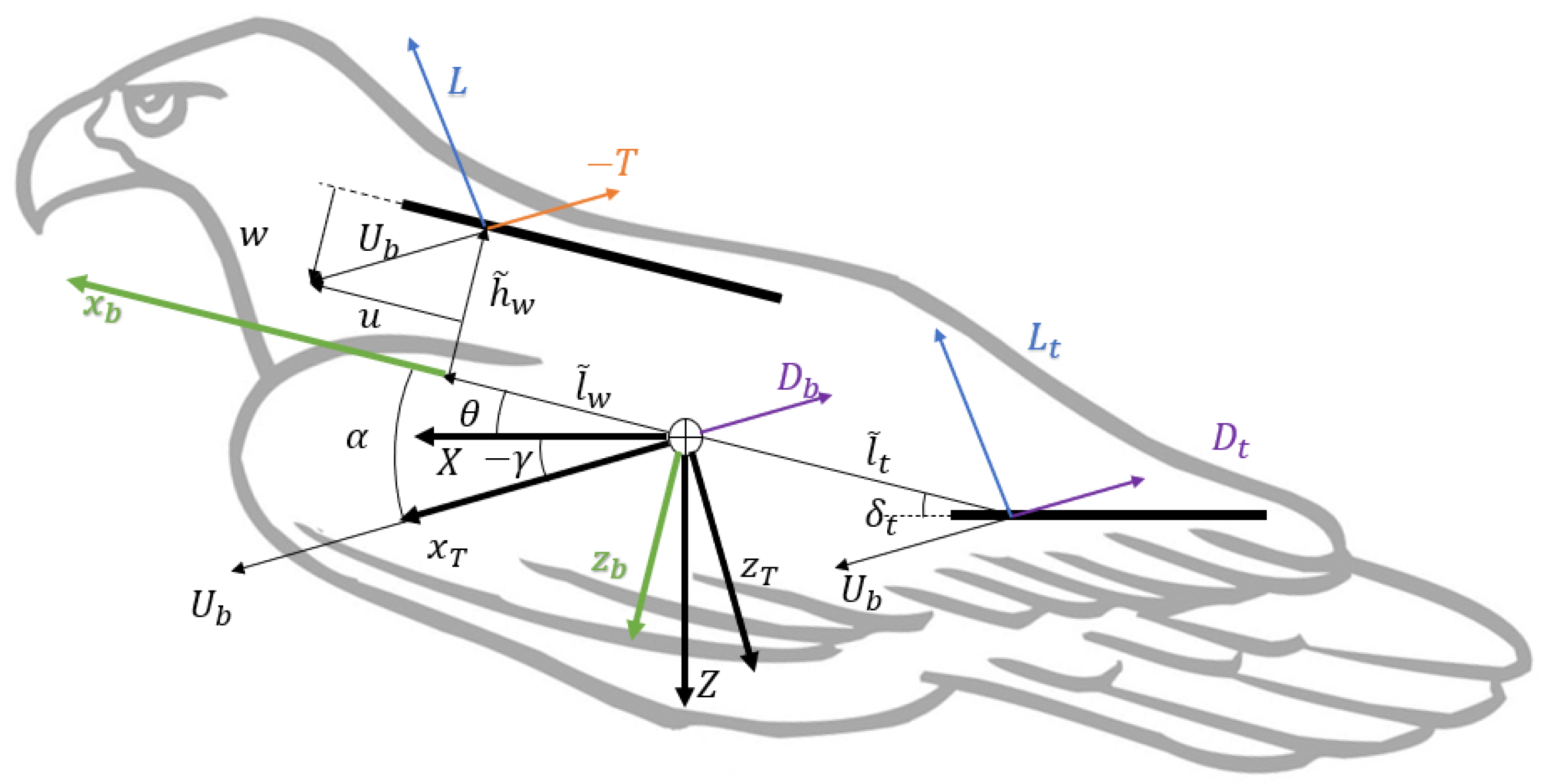
A sketch of the ornithopter with the different reference frames and the main (dimensional) parameters and state variables are provided in Figure 1. To simplify the problem, we use non-dimensional magnitudes scaled with the following characteristic velocity, length and time:

$$\begin{array}{c}\hfill \begin{array}{c}\hfill U_c=\sqrt{\frac{mg}{\pi \rho S{\delta }_t}},L_c=\frac{c}{2},t_c=\frac{1}{\omega },\end{array}\end{array}$$

(2)

where $U_c$ and $t_c$ are redefined from [27] to obtain a non-dimensional velocity of order unity in usual flapping conditions for a given tail deflection ${\delta }_t$, and a non-dimensional time in the order unity for flapping oscillations. Note that this formulation is only valid for the flapping mode of the ornithopter, as the flapping frequency is involved in the scaling of the dimensionless time.

During a longitudinal flight, one needs three dynamic equations: Two for the linear momentum on the plane of flight (X-Z, see Figure 1) and one for the angular momentum around the Y-axis perpendicular to this plane. They are written as [27], with some modifications

$$\mathcal{M}{k}_0\dot{U}=U^2\left(C_T^{*}-C_D^{*}-L{i}^{*}-\Lambda C_{Dt}^{*}\right)-{\delta }_{t}sin\left(\gamma \right),$$

(3)

$$\mathcal{M}{k}_{0}U\dot{\gamma }=U^2\left(C_L^{*}+\Lambda C_{Lt}^{*}\right)-{\delta }_{t}cos\left(\gamma \right),$$

(4)

$$\begin{array}{cc}\hfill {\left(\mathcal{M}{k}_0\right)}^2\ddot{\theta }& =\chi {\mathcal{M}}^2{U}^2\left\{l_w\left[C_L^{*}cos\left(\alpha \right)-(C_T^{*}-C_D^{*})sin\left(\alpha \right)\right]+l_t\Lambda \left[C_{Lt}^{*}cos\left(\alpha \right)+C_{Dt}^{*}sin\left(\alpha \right)\right]\right.\hfill \\ \hfill & \left.-h_w\left[C_L^{*}sin\left(\alpha \right)+\left(C_T^{*}-C_D^{*}\right)cos\left(\alpha \right)\right]\right\},\hfill \end{array}$$

(5)

and the wing’s angle of attack is computed as $\alpha =\theta -\gamma$. Equations (3)–(5) are written in the trajectory frame, with $x_T$ in the direction of the velocity. The non-dimensional parameters appearing in Equations (3)–(5) that differ from those used in [27] are

$$\begin{array}{c}\hfill \begin{array}{c}\hfill \mathcal{M}=\frac{2m}{\pi \rho Sc},\chi =\frac{\pi \rho S{\left(\frac{c}{2}\right)}^3}{2I_y},k_0=\frac{\omega c}{2U_c},\end{array}\end{array}$$

(6)

The (modified) force coefficients $C_L^{*}$, $C_T^{*}$, $C_D^{*}$, modeled in Section 2.2 are defined as

$$\begin{array}{c}\hfill \begin{array}{c}\hfill C_L^{*}=\frac{L}{\pi \rho U_b^{2}c},C_T^{*}=\frac{T}{\pi \rho U_b^{2}c},C_D^{*}=\frac{D}{\pi \rho U_b^{2}c},\end{array}\end{array}$$

(7)

applied at the wing aerodynamic center. The Lighthill number $L{i}^{*}=\frac{S_b}{S}{C}_{D_b}^{*}$, models the body drag, applied at the center of gravity. Small flapping amplitude is considered so that the wing aerodynamic center is assumed to be at a constant position ($l_w,h_w$) in the body frame. The force coefficients are dubbed modified because they are not defined in the traditional form but divided by $2\pi$ to better adjust the numerical order of magnitude of the different terms in the equations, as described in Section 4.

2.2. Aerodynamic Characterization

For the aerodynamic formulation, the movement of the wing is characterized by the non-dimensional flapping amplitude $h_0$ and the reduced (dimensionless) frequency, $k=\frac{k_0}{U}$, which is affected by the dynamics through the non-dimensional velocity U in relation to the constantly reduced frequency $k_0$, defined in (6).

Since we assume small flapping amplitudes, we use the well-known results from two-dimensional, linear potential theory, recently modified for the thrust coefficient and also corrected to account for three-dimensional effects. Thus, we use Theodorsen’s lift [10] for an oscillating, heaving-only two-dimensional airfoil but assume an angle of attack $\alpha \ne 0$ that may vary with time. In fact, all terms coming from changes in dynamic state variables are also considered as they have important effects on the stability of fixed-wing flight [27] and are also expected to affect the flapping flight.

To also account for three-dimensional effects, we follow recent works that separate the finite wing effects on the added mass terms and the circulatory terms of the lift force [15]. Circulatory terms are affected by the same factor used in fixed wings according to Prandtl’s lifting-line theory, namely /( + 2), where $=b^2/S$ is the aspect ratio of the wing. On the other hand, Smits [16] proposes a discontinuous factor for the added mass terms, with $/2$ for $<2$ and just unity for $\ge 2$. This last factor is the appropriate one for the wings considered here. We can write the (modified) lift coefficient as a function of the state variables:

$$\begin{array}{c}\hfill \begin{array}{c}\hfill C_L^{*}=C_{L_{\alpha }}\alpha +\frac{C_{L_h}{e}^{it}+{\overline{C}}_{L_h}{e}^{-it}}{U}{h}_0+\frac{C_{L_{\dot{\alpha }}}}{U}\dot{\alpha }+\frac{C_{L_{\dot{U}}}}{U^2}\alpha \dot{U}+\frac{C_{L_{\dot{\theta }}}}{U}\dot{\theta },\end{array}\end{array}$$

(8)

where we see the harmonic function related to the heaving motion multiplying $h_0$. The different coefficients $C_{L...}$ in Equation (8) (the dots refer to the different subscripts) are obtained from Theodorsen’s theory, and they are defined in Appendix A.

The formulation of the thrust for an oscillating airfoil in the linear potential limit was first obtained by Garrick [11]. The theoretical development has been recently corrected in [14] using the vortex impulse theory. This formulation for the thrust is used here. Finite wing effects from [15,16] are considered, resulting in

$$\begin{array}{c}{C}_T^{*}=\frac{C_{T_c}}{U^2}{h}_0^2+C_{T_{\alpha }}{\alpha }^2+\frac{C_{T_{h\alpha }}{e}^{it}+{\overline{C}}_{T_{h\alpha }}{e}^{-it}}{U}{h}_0\alpha +\frac{C_{T_h}{e}^{2it}+{\overline{C}}_{T_h}{e}^{-2it}}{U^2}{h}_0^2+\frac{C_{T_{h\dot{\alpha }}}{e}^{it}+{\overline{C}}_{T_{h\dot{\alpha }}}{e}^{-it}}{U^2}{h}_0\dot{\alpha }\\ +\frac{C_{T_{\dot{\theta }\dot{\alpha }}}}{U^2}\dot{\theta }\dot{\alpha }+\frac{C_{T_{\dot{\alpha }\alpha }}}{U}\dot{\alpha }\alpha +\frac{C_{T_{h\dot{\theta }}}{e}^{it}+{\overline{C}}_{T_{h\dot{\theta }}}{e}^{-it}}{U^2}{h}_0\dot{\theta }+\frac{C_{T_{\dot{\theta }\alpha }}}{U}\dot{\theta }\alpha +\frac{C_{T_{\dot{\theta }}}}{U^2}{\dot{\theta }}^2+\frac{C_{T_{\dot{U}\alpha }}}{U^2}{\alpha }^2\dot{U}.\end{array}$$

(9)

Note that the variation of the dynamic variables produces several cross terms. For an isolated wing in a wind tunnel with a heaving movement, just the first four terms of Equation (9) would be present. All the coefficients $C_{T...}$ (dots refer to the different subscripts in Equation (9)) are defined by the development of the formulation in [14], and they are also defined in Appendix A.

The second lifting surface of the ornithopter, the tail, provides stability and pitch control. To formulate the forces generated by this second surface, delta-wing theory is used [35]. Bio-inspired UAVs usually have a triangular tail with a reduced aspect ratio similar to those of birds, for which this theory has proven to be appropriate [36,37]. Consequently, the tail’s lift is modeled as [27]

$$\begin{array}{c}\hfill \begin{array}{c}\hfill C_{Lt}^{*}=C_{L{t}_{\alpha }}\left(\alpha -{\delta }_t\right)+\frac{C_{L{t}_{\dot{\theta }}}}{U}\dot{\theta }+\frac{C_{L{t}_{\dot{\alpha }}}}{U}\dot{\alpha }=\frac{{ℛ}_t}{4}\left(\alpha -{\delta }_t\right)-\frac{{ℛ}_t}{4}\frac{k_0{l}_t}{U}\dot{\theta }+\frac{3{ℛ}_t}{8}\frac{k_0}{U}\dot{\alpha },\end{array}\end{array}$$

(10)

Finally, drag from all parts of the vehicle has to be considered. Body drag, represented by the modified Lighthill number $L{i}^{*}$, is considered constant for the normal range of angles of attack. Meanwhile, for the wing and tail, drag is computed as the contributions of a friction drag, which is also considered constant in the range of applicability of the model, and an induced drag is associated with the corresponding lift coefficients $C_L^{*}$ and $C_{Lt}^{*}$, which is computed from finite wing theory. In summary,

$$C_D^{*}=C_{D0}^{*}+C_{Di}^{*},C_{Di}^{*}=\frac{2C_L^{*2}}{ℛ},$$

(11)

$$C_{Dt}^{*}=C_{D0t}^{*}+C_{Dit}^{*},C_{Dit}^{*}=\frac{2C_{Lt}^{*2}}{{ℛ}_t}.$$

(12)

3. Numerical Results and Experimental Validation

This section presents, in Section 3.1, some numerical results of the model equations to describe the structure of the solution, which will guide the timescales analysis of the perturbation solution developed in Section 4. Before that, in Section 3.2, these numerical results are validated against experimental data from the flapping flight of an ornithopter prototype developed within the GFIFFIN project [5].

3.1. Numerical Results

To obtain the dynamic evolution from the gliding condition to the final flapping state, the equations described in Section 2 are numerically integrated. We use the values of the parameters from the prototype described in [5], which are shown in

Table 1. Non-dimensional flight parameters for three flapping frequencies.

f	$\mathcal{M}{\mathit{k}}_0$	$\mathcal{M}$	${\mathcal{M}}^2\mathit{\chi }$	$\mathbf{\Lambda }$	${\mathit{l}}_{\mathit{w}}$	${\mathit{l}}_{\mathit{t}}\mathbf{\Lambda }$	${\mathit{h}}_{\mathit{w}}$	${\mathbf{Li}}^{*}$
2 Hz	$0.79$	$2.54$	$2.12$	$0.25$	$0.55$	$-1.16$	$0.38$	$0.0048$	$5.14$
5 Hz	$1.98$	$2.54$	$2.12$	$0.25$	$0.55$	$-1.16$	$0.38$	$0.0048$	$5.14$
7 Hz	$2.77$	$2.54$	$2.12$	$0.25$	$0.55$	$-1.16$	$0.38$	$0.0048$	$5.14$

for three flapping frequencies f relevant for bird-scale flight (actually, only $k_0$ depends on f). Note that they are of order unity, except for the friction drag ($L{i}^{*}$).

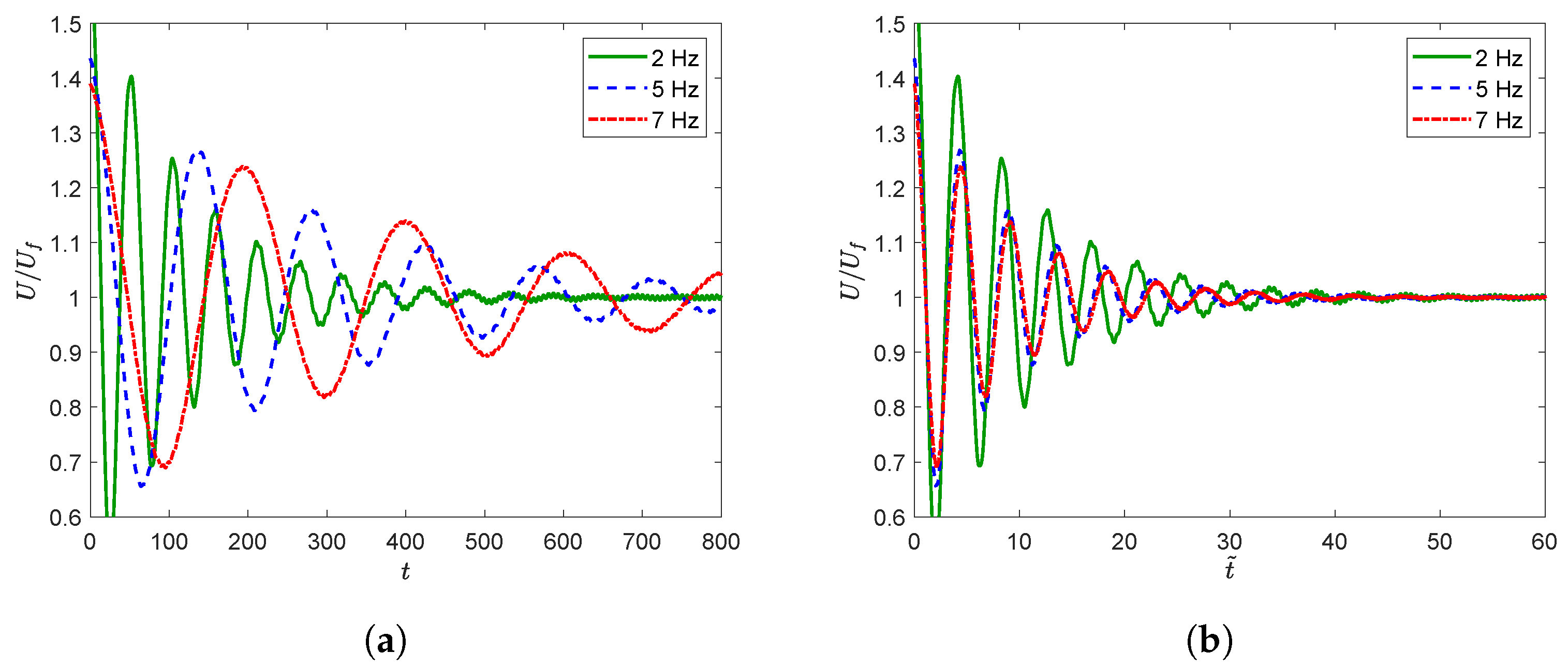
With these parameters, we proceed to numerically integrate the system of differential Equations (3)–(5). Figure 2 shows the evolution of the non-dimensional flight velocity U with both non-dimensional time (a) and dimensional time (b) for the three frequencies in Table 1. The flapping amplitude considered is $h_0=0.1$. To better compare the three cases, velocities have been normalized with their final values $U_f$, which are 0.9136, 1.0444 and 1.0792, respectively, and are all of order unity, as mentioned in Section 2.1. From Figure 2a, it is observed that the timescale of the transient phase increases with the frequency, while Figure 2b shows that the transient velocity is just slightly affected by the frequency when the dimensional time is used. Thus, though the timescale related to flapping oscillations is constant as a consequence of the non-dimensionalization of time with the flapping frequency, the timescale related to the transition between states varies with the frequency for the same reason.

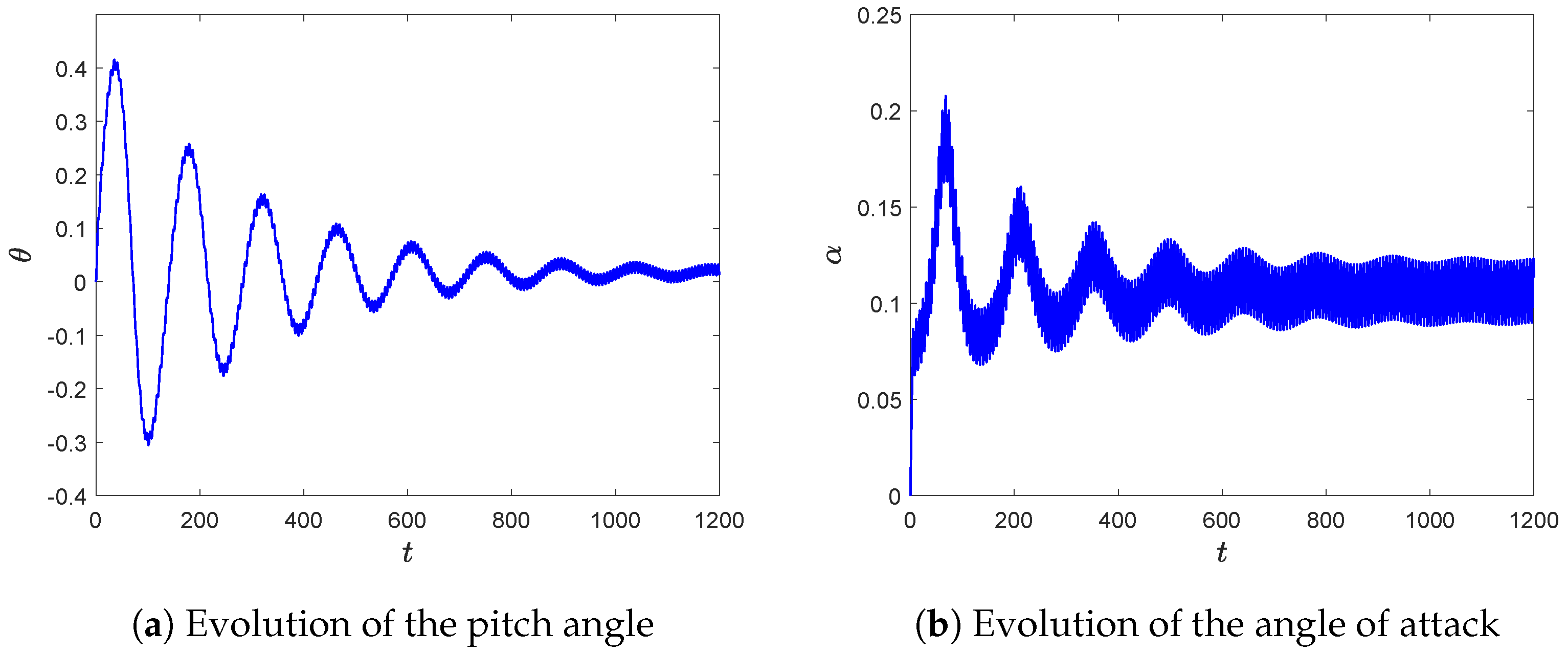
Figure 3 shows the evolution of the angular variables $\theta$ and $\alpha$ with time for a frequency of 5 Hz. Notice that the pitch angle amplitudes in the transient oscillations are significantly higher than those of the angle of attack. However, the oscillations due to the flapping motion are both quite similar. All the amplitudes, both in the transient oscillation and during each flapping cycle, are small enough to be in the adequate range for the aerodynamic models during the simulation [28,29,30,31]. Notice also that the aerodynamic models have no limitation in relation to the frequencies.

Numerical integration of the dynamic equations provides the most accurate tool to obtain the evolution of the state variables. However, state variables (velocity, pitch angle and angle of attack) oscillate with the flapping frequency but also evolve much more slowly in time during the transient phase. This disparity of timescales forces the numerical integration to be developed with a very small time step to accurately catch these oscillations, thus requiring a huge number of time steps to solve the slow evolution. Therefore, simulations of the entire transient phase have an excessive computational cost, which makes on-board real-time computations infeasible.

However, this same disadvantage associated with the different timescales can be used to develop simplifications of the model. Consequently, this paper proposes a perturbation approach (Section 4), separating scales with the flapping amplitude $h_0$ as the small parameter. The goal is to provide a system of equations that can be computed in real time by on-board computers.

3.2. Experimental Validation

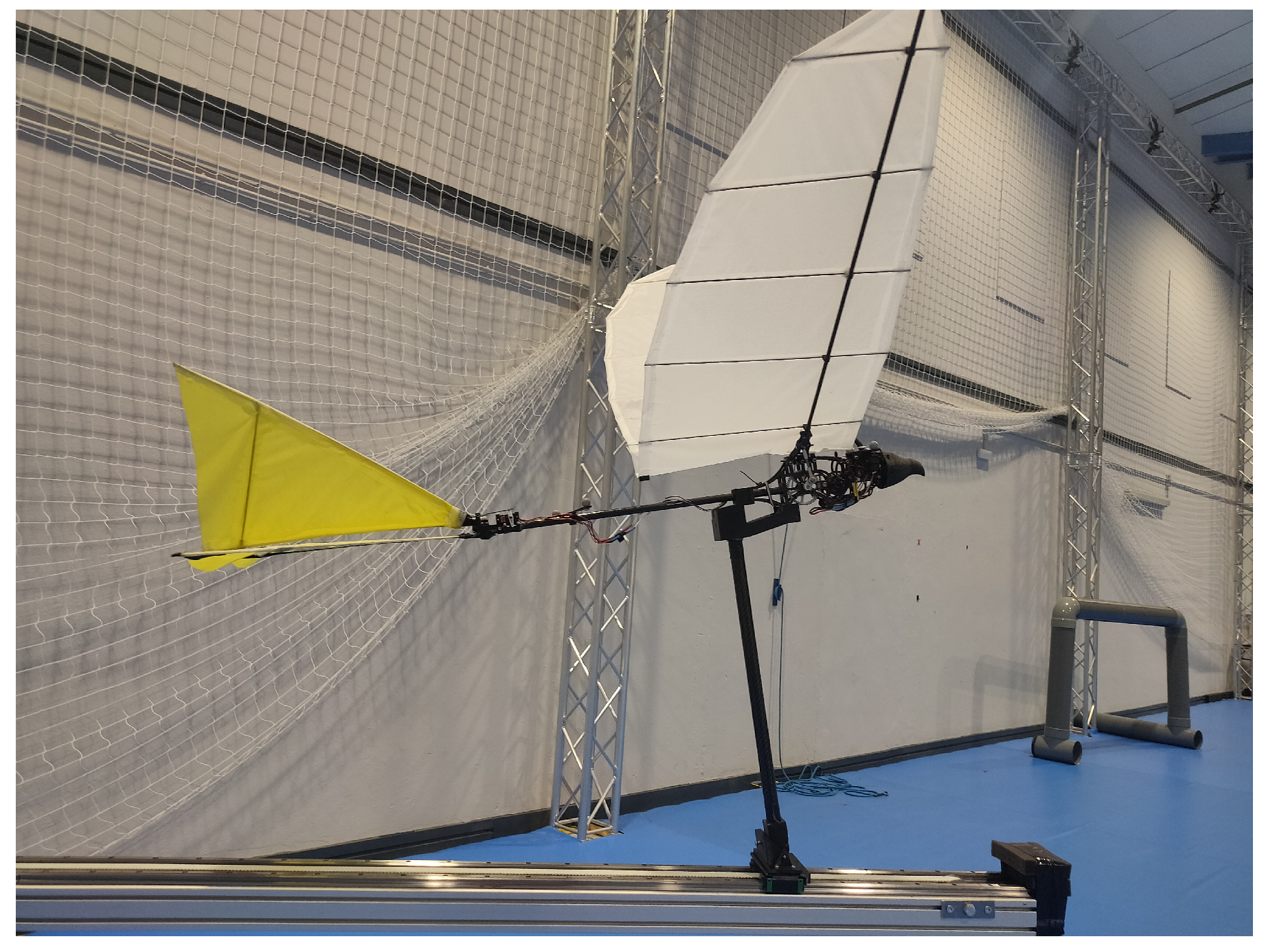
Experiments with the ornithopter prototype (described in [5]; see Figure 4) have been carried out in a 20 m $\times 15$ m tracking zone inside the GRVC Robotics Laboratory, with five markers on the body for the cameras to track the flight. The limited space of the flight area is inconvenient for achieving a long flight time, but its location inside a building without wind helps for the repeatability and reliability of the results. The lab is also equipped with a launcher to fix the initial conditions (also shown in Figure 4).

The prototype has a flapping amplitude $h_0\simeq 0.8$ (at $1/3$ of the semi-span from the wing tip), somewhat out of the range of the linear aerodynamics models. However, it has been shown that these models provide a good approximation of the aerodynamic forces even for these flapping amplitudes [14,28,29,30,31] (see also the present comparison with experimental data reported below in this section). Although the model does not take into account wing flexibility, the wing used here is more rigid than that reported in [5], and the effect of flexibility on the forces generated by the flapping wing is small for the flapping frequencies considered, which are much smaller than the characteristic frequency of the structure. Tail flexibility has not been considered either. In addition, due to the characteristics of the prototype’s tail, the coefficient $C_{L{t}_{\dot{\theta }}}$ is very small and is neglected.

There are three controls on the ornithopter. The vertical tail has a simple control to follow a straight line in the projection on the horizontal plane. We follow the diagonal of the flight area to maximize flight time. To consider the flight in open loop, the horizontal tail remains in a fixed position by sending a constant signal to the servomotor. The third control of the ornithopter generates the flapping frequency, which also receives a constant signal. However, this signal generates a constant current, which does not guarantee that the flapping motion is exactly harmonic, though the error in relation to a harmonic motion is shown to remain very small. The flapping frequency is not known a priori, but it can be extracted from the oscillations in the measured variables. We consider the flight from the moment the flight starts. Due to electronic delays, the ornithopter starts to fly between $0.5$ and 1 m forward from the launcher. The initial conditions change slightly from the launch to that point, so the conditions defined in the launcher are approximate.

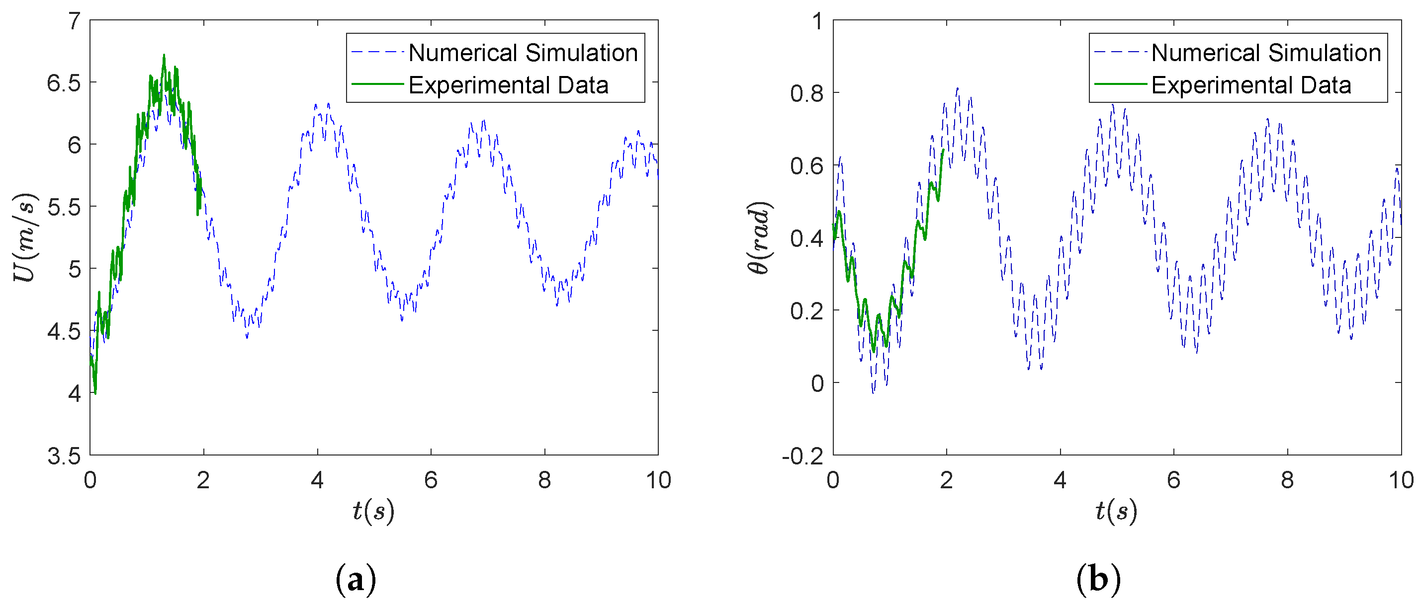
Figure 5 shows that the numerical results of the model for the flight velocity U and the pitch angle $\theta$ are very close to the experimental measurements. As we see, the flight time is only around 2 s due to the reduced space in the tracking zone. However, results for this short time flight are significant, as at least one transient oscillation is caught, with good agreement between experimental and theoretical frequencies and amplitudes of both fast (flapping) and transient scales. More particularly, the amplitude of the small oscillations with the flapping frequency have the same order for the airspeed, but they are slightly different for the pitch angle. This difference could be explained by the impact of the inertial forces, which would move the aerodynamic center of the wing backward, closer to the center of gravity. On the other hand, the first transient oscillation is very well captured by the model for both U and $\theta$.

4. Analytical Perturbation Solution and Its Comparison with the Numerical Solution

In this section, we present a perturbation solution to the model equations. First, in Section 4.1, the different timescales and orders of magnitude of the different parameters are analyzed with the help of the above numerical solutions and theoretical considerations. The solution is fully derived in Section 4.2 and then compared to the numerical results of the model equations in Section 4.3.

4.1. Scales Analysis

It is clear from the above numerical and experimental results that the problem has different timescales, so it seems appropriate to use a multiple-scale perturbation method, whose different temporal scales will be defined here in terms of the small flapping amplitude, $ϵ\equiv h_0\ll 1$. Before that, some assumptions have to be made regarding the order of magnitude, in terms of $ϵ$, of the non-dimensional variables and the remaining parameters for a typical ornithopter, which are enumerated next.

• Small flight angles: $\gamma \sim \theta \sim \alpha \sim {\delta }_t\sim ϵ$. Reduced angles of attack are required by the present aerodynamic formulation, as well as small deflections of the tail. All of them are assumed to be in the same order of magnitude as the flapping amplitude $ϵ$. Small $\gamma$ and $\theta$ mean that aggressive climbing trajectories are not considered. Moreover, small flapping amplitude implies a limited thrust, which is proportional to ${ϵ}^2$ (see below), so reaching large flight path angles would be possible only with high reduced frequencies, which are difficult to obtain in bird-scale ornithopters.
• Lift coefficients: $C_L^{*}\sim C_{Lt}^{*}\sim ϵ$. This is a consequence of the formulation of the lift coefficients, Equations (8) and (10), proportional to the aerodynamic angles and the flapping amplitude, as all the aerodynamic parameters are of order unity.
• Thrust coefficient: $C_T^{*}\sim {ϵ}^2$. Clearly from the Formulation (9), with products of the aerodynamic angles and the flapping amplitude.
• Drag coefficients: $C_D^{*}\sim C_{Dt}^{*}\sim L{i}^{*}\sim {ϵ}^2$. This is clear for the induced drag, as it is proportional to the square of the lift coefficient. On the other hand, friction drag cannot be larger than thrust to maintain flight.
• Non-dimensional inertia and reduced frequency: ${\mathcal{M}}^2\chi \sim \mathcal{M}{k}_0\sim 1$. Given in Table 1. Even though the frequency is a control variable, we can consider both terms of order unity in the typical range of bird-like ornithopters.
• All the remaining non-dimensional parameters either do not affect the structure of the solution or are order unity.

With these considerations, we can analyze the timescales. Two of them are clearly recognized in Figure 2. The first one, corresponding to the flapping oscillations, is of order unity (due to the definition of the characteristic time $t_c$). The order of magnitude of the other one, corresponding to the transient phase, can be obtained by analyzing the order of the different terms in Equations (3) and (4) during the transient phase. The asymptotic terms are neglected in this analysis as they are compensated by themselves. Thus, writing as $\Delta U/{\tau }_{c1}$ and $\Delta \gamma /{\tau }_{c1}$, the order of magnitude of the time derivatives, where ${\tau }_{c1}$ is the transient timescale in non-dimensional time t, one has

$$\mathcal{M}{k}_0{\displaystyle \frac{\Delta U}{{\tau }_{c1}}}\sim U(\Delta U){ϵ}^2+ϵ\Delta \gamma ,$$

(13)

$$\mathcal{M}{k}_{0}U{\displaystyle \frac{\Delta \gamma }{{\tau }_{c1}}}\sim U(\Delta U)ϵ+ϵ\gamma \Delta \gamma ,$$

(14)

where it has been taken into account that the leading terms with $U^2$ cancel with the corresponding gravity terms so that the velocity terms going with the aerodynamic coefficients in this transient phase are of the order of $U\Delta U$. Since $U\sim 1$ by the choice of $U_c$ and the characteristic time has to be of the same order in both equations (the numerical solutions plotted in Figure 2 and Figure 3 show a similar oscillatory convergence for U and for the angular variables), it necessarily implies that $\Delta U$ is of the same order as $\Delta \gamma$. Thus,

$$\mathcal{M}{k}_0{\displaystyle \frac{1}{{\tau }_{c1}}}\sim {ϵ}^2+ϵ,$$

(15)

$$\mathcal{M}{k}_0{\displaystyle \frac{1}{{\tau }_{c1}}}\sim ϵ+{ϵ}^2,$$

(16)

and, comparing the leading terms, ${\tau }_{c1}=\mathcal{M}{k}_0/ϵ$. These leading terms are related to the gravity force and to the effect of the velocity variations on the lift force. However, the damping terms related to the aerodynamic drag are negligible in this time scale. Thus, we have to consider yet another (slower) characteristic time to account for the drag term in (13),

$$\begin{array}{c}\hfill \begin{array}{c}\hfill \mathcal{M}{k}_0{\displaystyle \frac{\Delta U}{{\tau }_{c2}}}\sim U(\Delta U){ϵ}^2,\end{array}\end{array}$$

(17)

obtaining the third timescale ${\tau }_{c2}=\mathcal{M}{k}_0/{ϵ}^2$. Aerodynamic coefficient variations have not been considered as, even though they can affect the transient phase, they will not change the corresponding timescales.

Therefore, the complexity of the present problem needs three timescales to obtain a meaningful perturbation solution: t, ${\tau }_1=t/{\tau }_{c1}$, and ${\tau }_2=t/{\tau }_{c2}$. Non-dimensional time derivatives are thus defined as the sum of three terms

$$\begin{array}{c}\hfill \begin{array}{c}\hfill \frac{d}{dt}=\frac{\partial }{\partial t}+\frac{ϵ}{\mathcal{M}{k}_0}\frac{\partial }{\partial {\tau }_1}+\frac{{ϵ}^2}{\mathcal{M}{k}_0}\frac{\partial }{\partial {\tau }_2}.\end{array}\end{array}$$

(18)

The state variables can then be expressed as an asymptotic expansion in powers of $ϵ$,

$$U=U_0(t,{\tau }_1,{\tau }_2)+ϵU_1(t,{\tau }_1,{\tau }_2)+{ϵ}^2{U}_2(t,{\tau }_1,{\tau }_2)+\cdots$$

(19)

$$\theta =ϵ\left({\theta }_1(t,{\tau }_1,{\tau }_2)+ϵ{\theta }_2(t,{\tau }_1,{\tau }_2)+\cdots \right)$$

(20)

$$\alpha =ϵ\left({\alpha }_1(t,{\tau }_1,{\tau }_2)+ϵ{\alpha }_2(t,{\tau }_1,{\tau }_2)+\cdots \right)$$

(21)

Note that $\alpha$ is considered here as a state variable instead of the flight path angle $\gamma$ to simplify the integration of the aerodynamic forces in the dynamic equations. $\gamma$ can be expressed as the difference between the pitch angle and the angle of attack:

$$\gamma =ϵ\left[{\theta }_1(t,{\tau }_1,{\tau }_2)-{\alpha }_1(t,{\tau }_1,{\tau }_2)\right]+{ϵ}^2[{\theta }_2(t,{\tau }_1,{\tau }_2)-{\alpha }_2(t,{\tau }_1,{\tau }_2)]+\cdots$$

(22)

The dependence with each timescale of the different functions in the expansions is derived in Section 4.2 below. Additionally, since the first timescale t is related to harmonic oscillations with the flapping frequency, the different functions in Equations (19)–(21) will be expanded in Fourier series with the necessary number of terms to account for the aerodynamic forces (8) and (9). The harmonic terms are presented in their exponential form. To simplify the expressions, their conjugates are omitted for clarity purposes, but obviously they are included when implemented in the equations. In order to not repeat terms, the Fourier series coefficients of $U,\theta ,\alpha$ will be named with the capital letters $V,T,A$, with subscripts following the order in the expansion. For instance, the velocity terms will be expanded as follows,

$$U_0=V_0({\tau }_1,{\tau }_2)+V_1({\tau }_1,{\tau }_2)e^{it}+\cdots +V_n({\tau }_1,{\tau }_2)e^{int}$$

(23)

$$U_1=V_{n+1}({\tau }_1,{\tau }_2)+V_{n+2}({\tau }_1,{\tau }_2)e^{it}+\cdots +V_{n+k+1}({\tau }_1,{\tau }_2)e^{ikt}$$

(24)

where the number of terms in each order ($n,k,\cdots$) is given by the expansion of the equations in the next Section 4.2. These Fourier coefficients are complex, and to also include the phase of the oscillations, the real value needed for the evolution of the system is obtained by taking into account the corresponding complex conjugate.

4.2. Perturbation Solution

Once the expansions (19)–(21) and the time derivatives (18) have been defined, we apply the standard multiple-scales perturbation method to simplify the problem by separating Equations (3)–(5) into a set of simpler equations by equating similar powers of $ϵ$ [38].

In addition to the general perturbation scheme, we must consider the expansion in a Fourier series. Therefore, each equation obtained for a particular power of $ϵ$ can be divided into different equations with the harmonic functions as a common factor, obtaining equations with different harmonic terms ($e^0$, $e^{it}$, $e^{2it}$, …).

This procedure provides a set of simple algebraic equations for each power of $ϵ$ and for each specific harmonic term. At the lowest order $\mathcal{O}\left({ϵ}^0\right)=\mathcal{O}\left(1\right)$, just one term remains, belonging to Equation (3),

$$\begin{array}{c}\hfill \begin{array}{c}\hfill \frac{\partial U_0}{\partial t}=0\end{array}\end{array}$$

(25)

meaning that the lowest order of the velocity does not depend on the fast time variable t of the oscillations. This result agrees with the numerical solution in Figure 2, where we saw that the oscillations of the velocity with the flapping frequency have very small amplitude.

Following the mathematical development, at the next order $\mathcal{O}\left(ϵ\right)$, we obtain the following equations:

$$\begin{array}{cc}\hfill \frac{\partial U_0}{\partial {\tau }_1}+\frac{\partial U_1}{\partial t}& =0\hfill \end{array}$$

(26)

$$\begin{array}{cc}\hfill \mathcal{M}{k}_0{U}_0\left(\frac{\partial {\theta }_1}{\partial t}-\frac{\partial {\alpha }_1}{\partial t}\right)& =U_0^2\left(C_{L_{\alpha }}{\alpha }_1+\Lambda C_{L{t}_{\alpha }}\left({\alpha }_1-{\delta }_t^{*}\right)\right)\hfill \\ \hfill & +U_0\left(C_{L_h}{e}^{it}+\left(C_{L_{\dot{\theta }}}+\Lambda C_{L{t}_{\dot{\theta }}}\right)\frac{\partial {\theta }_1}{\partial t}+\left(C_{L_{\dot{\alpha }}}+\Lambda C_{L{t}_{\dot{\alpha }}}\right)\frac{\partial {\alpha }_1}{\partial t}\right)-{\delta }_t^{*}\hfill \end{array}$$

(27)

$$\begin{array}{cc}\hfill \frac{{\left(\mathcal{M}{k}_0\right)}^2}{{\mathcal{M}}^2\chi }\frac{{\partial }^2{\theta }_1}{\partial t^2}& =U_0^2\left(l_w{C}_{L_{\alpha }}{\alpha }_1+\Lambda l_t{C}_{L{t}_{\alpha }}\left({\alpha }_1-{\delta }_t^{*}\right)\right)\hfill \\ \hfill & +U_0\left(l_w{C}_{L_h}{e}^{it}+\left(l_w{C}_{L_{\dot{\theta }}}+\Lambda l_t{C}_{L{t}_{\dot{\theta }}}\right)\frac{\partial {\theta }_1}{\partial t}+\left(l_w{C}_{L_{\dot{\alpha }}}+\Lambda l_t{C}_{L{t}_{\dot{\alpha }}}\right)\frac{\partial {\alpha }_1}{\partial t}\right)\hfill \end{array}$$

(28)

From the first Equation (26), it follows that $U_1$ is also independent of the fast time t. Note that, according to (25), terms with $\partial U_0/\partial t$ disappear from Equations (27) and (28).

Now we separate Equations (26)–(28) by harmonic terms. First, non-oscillatory terms in Equations (26)–(28) generate a system of equations for the coefficients associated with the non-harmonic terms in the Fourier series. From (26), only $\partial U_0/\partial {\tau }_1=0$ remains, so that the lowest order velocity does not depend on ${\tau }_1$. With the other two equations, we have a system for the two variables $V_0$ and $A_0$, without any temporal derivative. Therefore, $A_0$ and $V_0$ are, in fact, constants, independent of any time variable, and are given by

$$A_0=\frac{l_t\Lambda C_{L{t}_{\alpha }}{\delta }_t^{*}}{l_w{C}_{L_{\alpha }}+l_t\Lambda C_{L{t}_{\alpha }}}$$

(29)

$$V_0=\sqrt{\frac{{\delta }_t^{*}}{C_{L_{\alpha }}{A}_0+C_{L{t}_{\alpha }}\Lambda \left(A_0-{\delta }_t^{*}\right)}}.$$

(30)

$C_{L_{\alpha }}$ depends on the velocity $V_0$ through the reduced frequency in Theodorsen’s function (see Equation (A1)). Note that only the lowest-order velocity has to be considered in Theodorsen’s function to be consistent with the present order of the expansion. In any case, this is a quite simple couple of algebraic equations for $A_0$ and $V_0$. These and all the other algebraic equations that will appear in the development of the perturbation method are solved numerically using Matlab’s function fsolve.

The number of terms in the Fourier series of each variable is limited by the equations, as discussed above. In this order of $ϵ$, Equation (26) has no oscillating terms for the variable $U_1$. Therefore, this variable does not depend on t, and we have that the two lower orders of the velocity only have the non-harmonic term from the Fourier series. Then, Equations (27) and (28) have oscillating terms with just the first mode, which leads to ${\theta }_1$ and ${\alpha }_1$ having only one oscillating term. The corresponding functions are obtained from the following system,

$$\begin{array}{cc}\hfill bluei\left(\mathcal{M}{k}_0-\left(C_{L_{\dot{\theta }}}+\Lambda C_{L{t}_{\dot{\theta }}}\right)\right)T_1-\left(i\mathcal{M}{k}_0+i\left(C_{L_{\dot{\alpha }}}+\Lambda C_{L{t}_{\dot{\alpha }}}\right)+V_0\left(C_{L_{\alpha }}+\Lambda C_{L{t}_{\alpha }}\right)\right)A_1& =C_{L_h}\hfill \end{array}$$

(31)

$$\begin{array}{cc}\hfill -\left(\frac{k_0^2}{\chi }+i{V}_0\left(l_w{C}_{L_{\dot{\theta }}}+\Lambda l_t{C}_{L{t}_{\dot{\theta }}}\right)\right)T_1-\left(V_0^2\left(l_w{C}_{L_{\alpha }}+\Lambda l_t{C}_{L{t}_{\alpha }}\right)+i{V}_0\left(l_w{C}_{L_{\dot{\alpha }}}+\Lambda l_t{C}_{L{t}_{\dot{\alpha }}}\right)\right)A_1& =l_w{V}_0{C}_{L_h}\hfill \end{array}$$

(32)

We see that the system of Equations (31) and (32) does not have any derivative with ${\tau }_1$ and ${\tau }_2$, so all terms are constants and, consequently, so are $A_1$ and $T_1$. Note that this is a complex algebraic system, as complex unit i appears with derivatives with variable t. Coefficients $A_1$ and $T_1$ are thus complex, giving information about the amplitudes of the oscillations $|T_1|$ and $|A_1|$ and their respective phases ${\varphi }_{T1}$ and ${\varphi }_{A1}$: $T_1=\left|T_1\right|e^{i{\varphi }_{T1}}$ and $A_1=\left|A_1\right|e^{i{\varphi }_{A1}}$.

In addition, there is also a transient mode with time scale t from Equations (26)–(28), given by

$$\begin{array}{cc}\hfill \left(-\mathcal{M}{k}_0-\left(C_{L_{\dot{\alpha }}}+\Lambda C_{L{t}_{\dot{\alpha }}}\right)\right)\frac{\partial {\alpha }_1}{\partial t}& =\left(\left(C_{L_{\dot{\theta }}}+\Lambda C_{L{t}_{\dot{\theta }}}\right)-\mathcal{M}{k}_0\right)\frac{\partial {\theta }_1}{\partial t}+V_0\left(C_{L_{\alpha }}+\Lambda C_{L{t}_{\alpha }}\right){\alpha }_1\hfill \end{array}$$

(33)

$$\begin{array}{cc}\hfill \frac{k_0^2}{\chi }\frac{{\partial }^2{\theta }_1}{\partial t^2}-V_0\left(l_w{C}_{L_{\dot{\alpha }}}+\Lambda l_t{C}_{L{t}_{\dot{\alpha }}}\right)\frac{\partial {\alpha }_1}{\partial t}& =V_0\left(l_w{C}_{L_{\dot{\theta }}}+\Lambda l_t{C}_{L{t}_{\dot{\theta }}}\right)\frac{\partial {\theta }_1}{\partial t}+V_0^2\left(l_w{C}_{L_{\alpha }}+\Lambda l_t{C}_{L{t}_{\alpha }}\right){\alpha }_1\hfill \end{array}$$

(34)

From these linear equations, a fast mode can be easily obtained. However, these transients are not of interest. To not alter the dynamics of the ornithopter, we just have to ensure that these fast solutions are stable.

Summarizing, order $ϵ$ of the equation provides information about the lowest order of the three variables. For the velocity, we have the (constant) only term of $U_0$, knowing also that $U_1$ does not have any harmonic oscillation with t. For the pitch angle, we have the harmonic oscillations with t of ${\theta }_0$. Finally, all the terms of ${\alpha }_0$ are already known.

There is not enough information to obtain the evolution of the system yet, so we have to analyze the order ${ϵ}^2$ of the equations. Each Fourier coefficient in this order is expected to have an asymptotic value and a transient term. To simplify the system further, each coefficient is decomposed as $X({\tau }_1,{\tau }_2)=X_s+X_t({\tau }_1,{\tau }_2)$ from this point onwards to divide it into two separate systems of equations. Firstly, for the constant terms (with subscripts s), the following analytical expressions are obtained

$$\begin{array}{cc}\hfill T_{0s}& =A_0+{\displaystyle \frac{V_0^2}{{\delta }_t^{*}}}\left(\left(C_{T_{\alpha }}-\Lambda C_{D{t}_{\alpha }}\right)\left(A_0^2+2A_1{\overline{A}}_1\right)-\Lambda C_{D{t}_{\alpha {\delta }_t}}{\delta }_t^{*}{A}_0-C_{D_0}^{*}-L{i}^{*}-\Lambda C_{D_{0t}}^{*}\right)\hfill \\ \hfill & +{\displaystyle \frac{V_0}{{\delta }_t^{*}}}\left(C_{T_{h\alpha }}{\overline{A}}_1+{\overline{C}}_{T_{h\alpha }}{A}_1+C_{T_{\dot{\theta }\alpha }}\left(i{T}_1{\overline{A}}_1-i{\overline{T}}_1{A}_1\right)\right)+\frac{i}{{\delta }_t^{*}}\left({\overline{C}}_{T_{h\dot{\alpha }}}{A}_1-C_{T_{h\dot{\alpha }}}{\overline{A}}_1\right)\hfill \\ \hfill & +\frac{C_{T_{\dot{\theta }\dot{\alpha }}}}{{\delta }_t^{*}}\left(A_1{\overline{T}}_1+{\overline{A}}_1{T}_1\right)+\frac{i}{{\delta }_t^{*}}\left({\overline{C}}_{T_{h\dot{\theta }}}{T}_1-C_{T_{h\dot{\theta }}}{\overline{T}}_1\right)+\frac{2C_{T_{\dot{\theta }}}{T}_1{\overline{T}}_1}{{\delta }_t^{*}}+\frac{C_{T_c}}{{\delta }_t^{*}}\hfill \end{array}$$

(35)

$$\begin{array}{cc}\hfill A_{2s}& =\frac{h_w}{l_w{C}_{L_{\alpha }}+\Lambda l_t{C}_{L{t}_{\alpha }}}\left(\left(C_{T_{\alpha }}+C_{L_{\alpha }}\right)\left(A_0^2+2A_1{\overline{A}}_1\right)-C_{D_0}^{*}\right.\hfill \\ \hfill & +\frac{1}{V_0}\left((C_{T_{h\alpha }}+C_{L_h}){\overline{A}}_1+({\overline{C}}_{T_{h\alpha }}+{\overline{C}}_{L_h})A_1+(C_{T_{\dot{\theta }\alpha }}+C_{L_{\dot{\theta }}})\left(i{T}_1{\overline{A}}_1-i{\overline{T}}_1{A}_1\right)\right)\hfill \\ \hfill & \left.+\frac{1}{V_0^2}\left(i\left({\overline{C}}_{T_{h\dot{\alpha }}}{A}_1-C_{T_{h\dot{\alpha }}}{\overline{A}}_1\right)+C_{T_{\dot{\theta }\dot{\alpha }}}\left(A_1{\overline{T}}_1+{\overline{A}}_1{T}_1\right)+i\left({\overline{C}}_{T_{h\dot{\theta }}}{T}_1-C_{T_{h\dot{\theta }}}{\overline{T}}_1\right)+2C_{T_{\dot{\theta }}}{T}_1{\overline{T}}_1+C_{T_c}\right)\right)\hfill \end{array}$$

(36)

$$\begin{array}{cc}\hfill V_{1s}& =-A_{2s}\frac{V_0}{2}\frac{C_{L_{\alpha }}+\Lambda C_{L{t}_{\alpha }}}{C_{L_{\alpha }}{A}_0+C_{L{t}_{\alpha }}\Lambda \left(A_0-{\delta }_t^{*}\right)}\hfill \end{array}$$

(37)

which are easily computed using the terms defined or obtained above. These constant terms provide the asymptotic values to be reached by each state variable after the transient mode at the corresponding order of the expansion.

For the transient terms, which depend on the time variables ${\tau }_1$ and ${\tau }_2$, we obtain

$$\frac{d{V}_{1t}({\tau }_1,{\tau }_2)}{d{\tau }_1}=-{\delta }_t^{*}{T}_{0t}({\tau }_1,{\tau }_2)$$

(38)

$$\frac{d{T}_{0t}({\tau }_1,{\tau }_2)}{d{\tau }_1}=\frac{2V_{1t}({\tau }_1,{\tau }_2)\left(C_{L_{\alpha }}{A}_0+C_{L{t}_{\alpha }}\Lambda \left(A_0-{\delta }_t^{*}\right)\right)}{1-{\displaystyle \frac{C_{L_{\dot{\theta }}}+\Lambda C_{L{t}_{\theta }}}{\mathcal{M}{k}_0}}+{\displaystyle \frac{l_w{C}_{L_{\dot{\theta }}}+l_t\Lambda C_{L{t}_{\dot{\theta }}}}{\mathcal{M}{k}_0}}{\displaystyle \frac{C_{L_{\alpha }}+\Lambda C_{L{t}_{\alpha }}}{l_w{C}_{L_{\alpha }}+l_t\Lambda C_{L{t}_{\alpha }}}}}$$

(39)

$$A_{2t}({\tau }_1,{\tau }_2)=-\frac{d{T}_{0t}({\tau }_1,{\tau }_2)}{d{\tau }_1}\frac{l_w{C}_{L_{\dot{\theta }}}+\Lambda l_t{C}_{L{t}_{\dot{\theta }}}}{\mathcal{M}{k}_0{V}_0\left(l_w{C}_{L_{\alpha }}+\Lambda l_t{C}_{L{t}_{\alpha }}\right)}$$

(40)

which is a system of two linear differential equations and a third algebraic expression for the evolution of the angle of attack. The solution to this system of ordinary differential equations has the form $X({\tau }_1,{\tau }_2)=e^{\lambda {\tau }_1}X\left({\tau }_2\right)$, where $\lambda$ turns out to be imaginary, $\lambda =i{\omega }_1$, representing a purely oscillating transient phase with frequency

$$\begin{array}{c}\hfill \begin{array}{c}\hfill {\omega }_1=\sqrt{2{\delta }_t^{*}\frac{C_{L_{\alpha }}{A}_0+C_{L{t}_{\alpha }}\Lambda \left(A_0-{\delta }_t^{*}\right)}{1-{\displaystyle \frac{C_{L_{\dot{\theta }}}+\Lambda C_{L{t}_{\theta }}}{\mathcal{M}{k}_0}}+{\displaystyle \frac{l_w{C}_{L_{\dot{\theta }}}+l_t\Lambda C_{L{t}_{\dot{\theta }}}}{\mathcal{M}{k}_0}}{\displaystyle \frac{C_{L_{\alpha }}+\Lambda C_{L{t}_{\alpha }}}{l_w{C}_{L_{\alpha }}+l_t\Lambda C_{L{t}_{\alpha }}}}}}\end{array}\end{array}$$

(41)

related to the mean lift of the ornithopter ($C_{L_{\alpha }}$) and the aerodynamic coefficient associated with the pitch angular velocity. It is observed that the frequency of this transient phase is not affected by the flapping frequency, in agreement with the numerical results shown in Section 3.1.

Given the form of the solution, the functions of ${\tau }_2$ that remain to be solved are complex, as they also include the information related to the phase of the oscillations. However, we can write them as real variables computing their phases separately and by using Equation (38) and the initial values $U_i$ and $T_i$ to yield

$$i{\omega }_1{e}^{i{\varphi }_V}{V}_{1t}\left({\tau }_2\right)=-e^{i{\varphi }_T}{\delta }_t^{*}{T}_{0t}\left({\tau }_2\right)$$

(42)

$${\varphi }_V-\frac{\pi }{2}={\varphi }_T,V_{1t}\left({\tau }_2\right)={\delta }_t^{*}\frac{T_{0t}\left({\tau }_2\right)}{{\omega }_1}$$

(43)

$$tan{\varphi }_T=\frac{-{\omega }_1{U}_i}{{\delta }_t^{*}{T}_i}$$

(44)

Equation (43) gives the relations between phases and amplitudes of the two variables obtained from Equation (42). The phase is determined by the initial conditions, as in Equation (44), and the phase shift is always 90 deg. This transient mode is common for aircraft and is known as phugoid mode. For the evolution with ${\tau }_2$, just another equation is needed, as the relation between $V_{1t}\left({\tau }_2\right)$ and $T_{0t}\left({\tau }_2\right)$ is already known.

Regarding the harmonic terms at the order ${ϵ}^2$ of Equations (3)–(5), both first and second-frequency terms, i.e., proportional to $e^{it}$ and $e^{2it}$, appear in the equations. Hence, the three variables $U_2$, ${\theta }_1$ and ${\alpha }_1$ have three terms in the Fourier series expansion. Considering Equation (3), the two resulting velocity coefficients are

$$\begin{array}{cc}\hfill V_3& =\frac{-i}{\mathcal{M}{k}_0}\left(V_0^2\left(\left(C_{T_{\alpha }}-\Lambda C_{D{t}_{\alpha }}\right)2A_0{A}_1-\Lambda C_{D{t}_{\alpha {\delta }_t}}{\delta }_t^{*}{A}_1\right)+V_0{A}_0\left(C_{T_{h\alpha }}+i{C}_{T_{\dot{\alpha }\alpha }}{A}_1+i{C}_{T_{\dot{\theta }\alpha }}{T}_1\right)-{\delta }_t^{*}{T}_1+{\delta }_t^{*}{A}_1\right)\hfill \end{array}$$

(45)

$$\begin{array}{cc}\hfill V_4& =\frac{-i}{2\mathcal{M}{k}_0}\left(V_0^2{A}_1^2\left(C_{T_{\alpha }}-\Lambda C_{D{t}_{\alpha }}\right)+V_0{A}_1\left(C_{T_{h\alpha }}+i{C}_{T_{\dot{\alpha }\alpha }}{A}_1+i{C}_{T_{\dot{\theta }\alpha }}{T}_1\right)+C_{T_h}+i{C}_{T_{h\dot{\alpha }}}{A}_1-C_{T_{\dot{\theta }\dot{\alpha }}}{A}_1{T}_1+i{C}_{T_{h\dot{\theta }}}{T}_1\right.\hfill \\ \hfill & -\left.C_{T_{\dot{\theta }}}{T}_1^2\right)\hfill \end{array}$$

(46)

Note that these lowest-order oscillations do not depend on the transient timescale, and they are constant during the entire evolution of the system. Furthermore, unlike the lowest-order oscillations for the pitch angle and the angle of attack considered above, both first and second-frequency oscillations appear in the velocity.

The oscillatory terms from (4) and (5) lead to the coefficients $A_3$ and $T_3$ for the harmonic term $e^{it}$, and $A_4$ and $T_4$ for $e^{2it}$. However, the analysis is algebraically more involved, as summarized in Appendix B. As it happens with coefficients $V_1$, $T_0$ and $A_2$, $A_3$ and $T_3$ contain steady and transient terms.

Finally, to obtain $T_{0t}\left({\tau }_2\right)$ and $V_{1t}\left({\tau }_2\right)$, order ${ϵ}^3$ of Equations (3)–(5) has to be considered. In this case, variables of higher order with the frequency ${\omega }_1$ appear. When combining the three equations for the transient non-harmonic terms, a single differential equation is obtained for the evolution of $T_{0t}\left({\tau }_2\right)$ (or alternatively $V_{1t}\left({\tau }_2\right)$). The result is written as $T_{0t}\left({\tau }_2\right)=T_i{e}^{(i{\omega }_2-\xi ){\tau }_2}$. The expressions for ${\omega }_2$ and $\xi$ are found in Appendix B.

4.3. Comparison between Analytical and Numerical Results

The theoretical approach developed allows a complete characterization of flapping forward flight. In contrast to other previous works [18,39], it also takes into account oscillations in state variables due to flapping wing movement, with a simplified model appropriate for on-board computers. This section presents a comparison between analytical and numerical results, showing their excellent agreement.

In summary, the analytical results obtained in the previous section are the following:

• For the large-time asymptotic values of the velocity and the pitch angle, we consider terms up to order ${ϵ}^2$, while for the angle of attack, the approximation is even better, up to order ${ϵ}^3$.
• Transient terms are computed up to order $ϵ$ for the velocity and the pitch angle, and to order ${ϵ}^2$ for the angle of attack.
• Harmonic oscillations with the flapping frequencies are considered up to order ${ϵ}^2$ for the three variables, including asymptotic and transient values.

Mathematically, the analytical solution used in the comparison is (the different constants and functions are obtained in Section 4.2 or Appendix B):

$$U\sim V_0+ϵ\left(V_{1s}+V_{1t}({\tau }_1,{\tau }_2)\right)+{ϵ}^2\left(V_{2s}+V_3{e}^{it}+V_4{e}^{2it}\right),$$

(47)

$$\theta \sim ϵ\left(T_{0s}+T_{0t}({\tau }_1,{\tau }_2)+ϵT_1{e}^{it}\right)+{ϵ}^2\left(T_{2s}+T_3({\tau }_1,{\tau }_2)e^{it}+T_4({\tau }_1,{\tau }_2)e^{2it}\right),$$

(48)

$$\alpha \sim ϵ\left(A_0+A_1{e}^{it}\right)+{ϵ}^2\left(A_{2s}+A_{2t}({\tau }_1,{\tau }_2)+A_3({\tau }_1,{\tau }_2)e^{it}+A_4({\tau }_1,{\tau }_2)e^{2it}\right)+{ϵ}^3{A}_{5s}.$$

(49)

Physically, the large-time permanent state consists of an oscillation of the variables in the fast timescale t (i.e., with the flapping frequency and some of its higher harmonics) around a steady value. The perturbation approach gives a low amplitude of the airspeed oscillations compared to its average value. The transient phase occurs in the slowest timescale ${\tau }_2$, while the period of the oscillations in the convergence towards the permanent state is of the order of the intermediate timescale ${\tau }_1$.

We present three different comparisons between the analytical perturbation solution and the numerical results: for the permanent state, for the transient phase and for the resulting trajectories. All the reported computations are for a frequency of 5 Hz, an amplitude $ϵ=h_0=0.1$, and a tail deflection of $4^{\circ }$. Similar results have been obtained for frequencies between 2 and 7 Hz, amplitudes between $0.05$ and $0.3$, and tail deflections between $0.5^{\circ }$ and ${10}^{\circ }$. Limits are fixed by aerodynamic theory for both amplitude and tail deflection. The frequency range is based on existing prototypes [5].

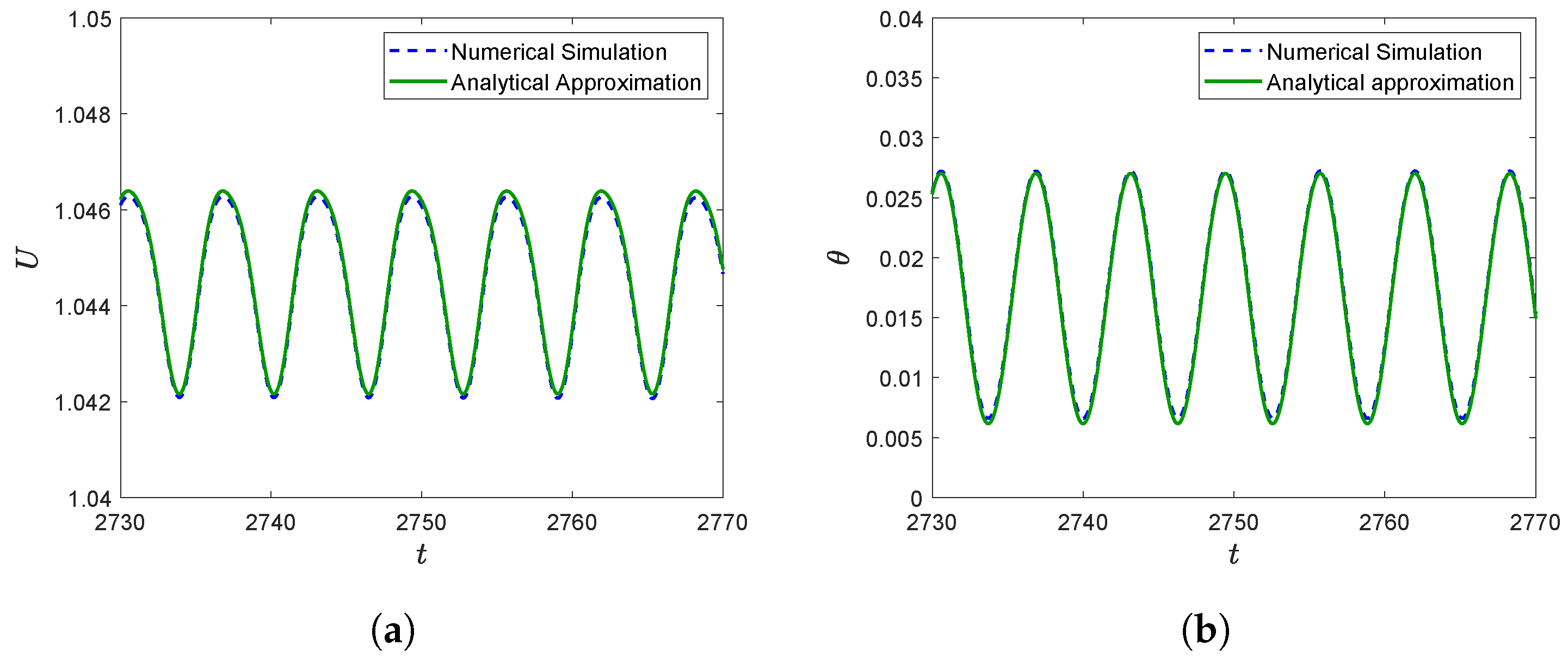
Figure 6 shows a good agreement between the numerical results and the analytical solution (47)–(49) for the large-time permanent state. Differences are of one order higher than that of the last term considered in (47)–(49), so we can conclude the validity of the analytical method for the given conditions. Figure 6a also assesses some of the hypotheses proposed for the simplified method, namely the order unity of the asymptotic airspeed and the order ${ϵ}^2$ of its oscillation amplitude. The minimal error of the perturbation solution for U does not suppose a significant difference in the trajectory followed by the UAV, and for long trajectories, it does not cause a larger error than that originated by inaccuracies in the measurement of the UAV characteristics. On the other hand, Figure 6b corroborates that the time-averaged value of the pitch angle is of the same order as the amplitude of its oscillations (their actual values in this case are even smaller than $O\left(ϵ\right)$), showing an excellent agreement between the analytical prediction and the numerical solution.

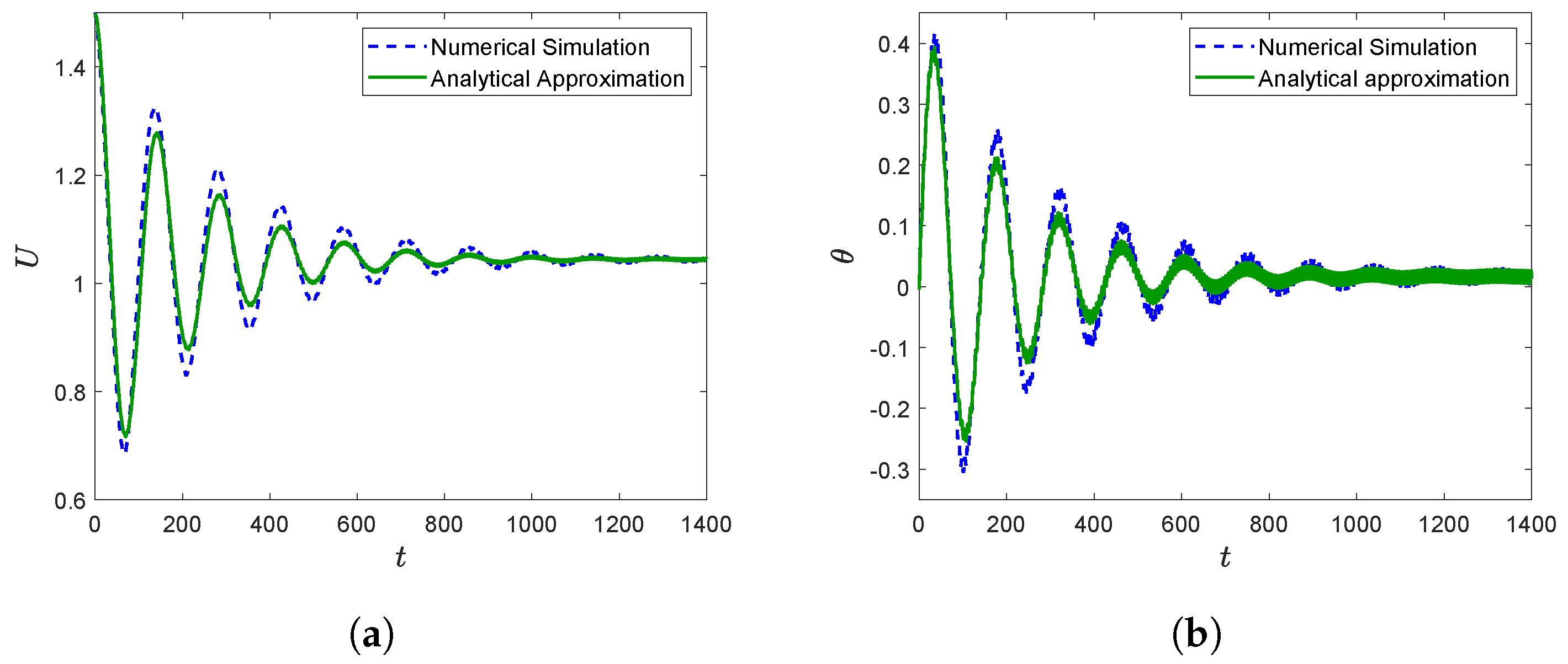
Figure 7 compares the transient phase for both the velocity and the pitch angle. Note the similarity in the shape of both transient phases, indicating the good adjustment of the timescales. However, the agreement with the numerical results of the transient phase is not as good as the one observed for the permanent flapping state in Figure 6. We also see how the orders considered in Section 3.1 are correct, with the transient velocity one order lower than its asymptotic value. On the other hand, the transient component of the pitch angle is of order $ϵ$, even though its asymptotic value is smaller in this particular case. Notice also that the amplitudes of the pitch oscillations remain in the adequate range for the reasonable application of the aerodynamic models.

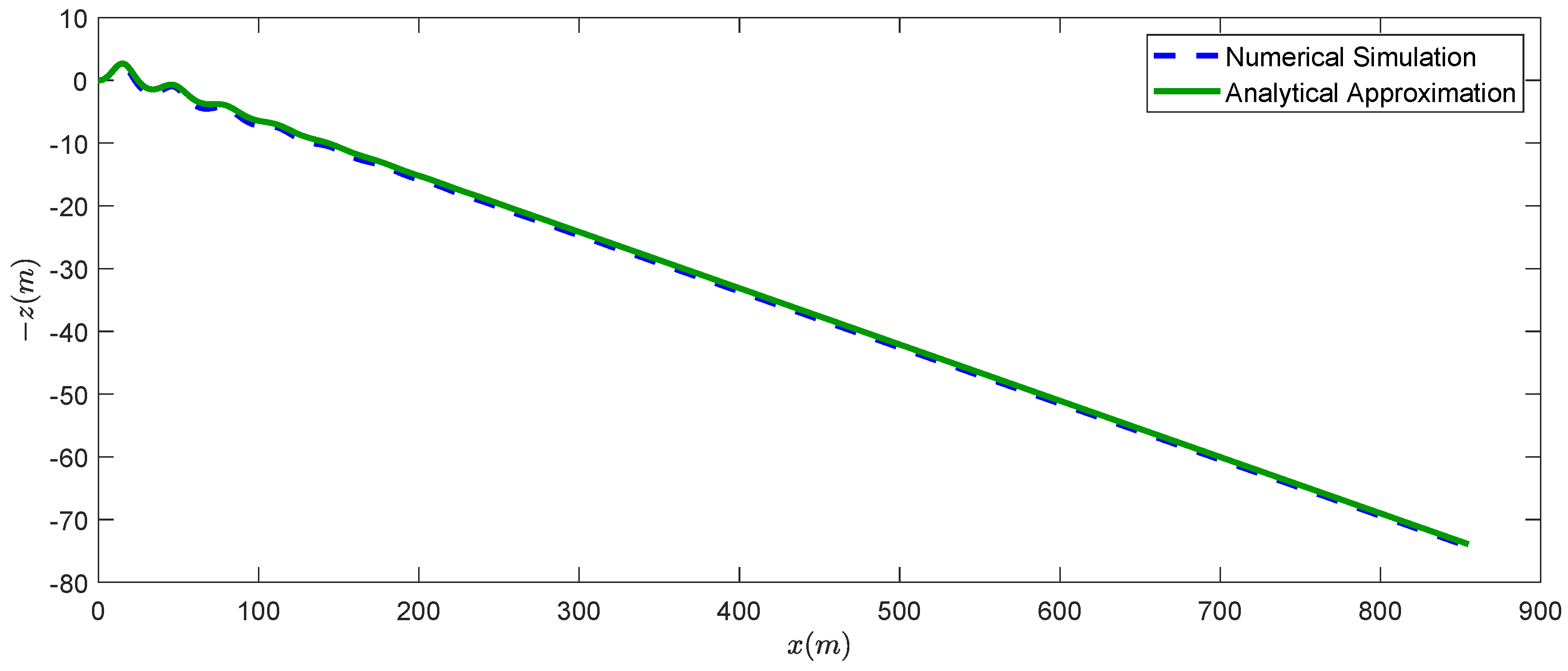
Figure 8 shows how the error in the transient approximation is not important for the trajectories, accumulating just a very small error in the large-time longitudinal path. Note how the thrust provided by the wing in this particular case is not enough to climb up, and the ornithopter follows a descending trajectory. To achieve more aggressive trajectories, an additional pitching movement would have to be included with the flapping motion. Most prototypes include this movement, either by an active pitching mechanism or by means of wing flexibility.

5. Summary and Conclusions

A new physical model for the forward flight of flapping wing UAVs has been presented. The model is restricted to low-amplitude flapping, appropriate for UAV cruising, using results from potential aerodynamic theory. Wholly unsteady aerodynamics models are employed instead of the quasi-steady approximations normally used [18,25], obtaining a more precise characterization of the non-stationary forces generated by the flapping wings. This new model is general for any bird-like ornithopter with a simple flapping (heaving) motion, and its results are validated with experimental data from the longitudinal flight of an ornithopter prototype.

The low-amplitude flapping approximation allows simplifications of the dynamic characteristics of the ornithopter. However, the numerical simulations with the model still have a high computational cost due to the small time step needed to accurately capture the flapping oscillations along very long transient periods. The resources needed for real-time on-board computations would exceed the limited payload of ornithopters. Hence, this paper proposes a simplification using multiple-scale perturbation methods in terms of the small flapping amplitude. The solution consists of a transient oscillatory phase, which converges to an asymptotic oscillatory regime with a much smaller amplitude and a much larger flapping frequency. Thus, the perturbation solution is built up with three timescales, the shortest one associated with the flapping frequency and an intermediate one corresponding to the transient oscillations towards the long-time behavior, which is reached in a much slower timescale. The perturbation solution is obtained analytically up to the second and third order in the small parameter, depending on the state variable.

In addition to its utility for on-board computations in real-time for trajectory planning and control, the analytical solution presented here is of interest, providing a simple and straightforward characterization of the final flapping-flight cruising state.

The validity of the approach is assessed by comparing it with numerical results previously validated against experimental data. It is shown that the large-time asymptotic values are very well caught by the approximate solution for both the main values and the amplitude and phase of the oscillations. The approximate solution for the transient phase proves the validity of the selected timescales, although its agreement with the exact numerical solution is less accurate. However, the final accumulative error in the trajectory is very small, as the larger transient errors disappear as the asymptotic values are reached.

The model is limited to bird-scale flapping-wing robots for the assumptions made on the order of magnitude of the variables to be valid. These assumptions are essential for the adequate development of the perturbation method. A different scaling would lead to changes in the perturbation equations. Thus the model may fail for very small robots such as hummingbirds and insect-like UAVs.

Another limitation is associated with the aerodynamic theory used, valid for small angles of attack and low-amplitude flapping. However, the models for the aerodynamic forces used here have been previously validated with experimental results, showing good agreement even for not-so-small flapping amplitudes in the present case of heaving motion [14,28,29,30,31], and the results of the dynamic equations with these aerodynamic models have been validated in the present work against experimental measurements of the longitudinal flapping flight of an ornithopter prototype.

Additionally, a rigid wing with just a flapping (heaving) movement is considered. Pitching, both active and/or passive by flexibility, is usual for bird-like vehicles because, as also shown here, flapping rigid wings produce limited thrust. With such low thrust, ornithopters need a very low drag to maintain sustained flight. Therefore, a combination of pitching and flapping movements is the most interesting path to extend this work. Considering both active pitching mechanisms and passive flexibility pitching, the model would be effective for all actual designs of flapping wing bird-like UAVs.

Finally, it is worth mentioning that another interesting path to extend this work would be the inclusion of lateral dynamics. Ornithopters do not usually turn like fixed-wing aircrafts, as the inclusion of anti-symmetrical control on the wing causes high mechanical complexity, especially in bird-sized UAVs. Then, most of them rely on tail configurations to control the lateral trajectory, obtaining different dynamics from those of conventional aircraft.

References

- Mueller, T.J. Fixed and Flapping Wing Aerodynamics for Micro Air Vehicle Applications; AIAA: Notre Dame, IN, USA, 2001. [Google Scholar]
- Gerdes, J.; Holness, A.; Perez-Rosado, A.; Roberts, L.; Greisinger, A.; Barnett, E.; Kempny, J.; Lingam, D.; Yeh, C.H.; Bruck, H.A.; et al. Robo Raven: A flapping-wing air vehicle with highly compliant and independently controlled wings. Soft Robot. 2014, 1, 275–288. [Google Scholar] [CrossRef]
- Srigrarom, S.; Chan, W.-L. Ornithopter Type Flapping Wings for Autonomous Micro Air Vehicles. Aerospace 2015, 2, 235–278. [Google Scholar] [CrossRef] [Green Version]
- Folkertsma, G.A.; Straatman, W.; Nijenhuis, N.; Venner, C.H.; Stramigioli, S. Robird: A robotic bird of prey. IEEE Robot. Autom. Mag. 2017, 24, 22–29. [Google Scholar] [CrossRef]
- Zufferey, R.; Tormo-Barbero, J.; Guzmán, M.M.; Maldonado, F.J.; Sanchez-Laulhe, E.; Grau, P.; Pérez, M.; Acosta, J.Á.; Ollero, A. Design of the High-Payload Flapping Wing Robot E-Flap. IEEE Robot. Autom. Lett. 2021, 6, 3097–3104. [Google Scholar] [CrossRef]
- Grauer, J.; Ulrich, E.; Hubbard, J., Jr.; Pines, D.; Humbert, J.S. Testing and system identification of an ornithopter in longitudinal flight. J. Aircr. 2011, 48, 660–667. [Google Scholar] [CrossRef]
- Taha, H.; Hajj, M.R.; Nayfeh, A. Flight dynamics and control of flapping-wing MAVs: A review. Nonlinear Dyn. 2012, 70, 907–939. [Google Scholar] [CrossRef]
- Wang, Z.J. Dissecting insect flight. Annu. Rev. Fluid Mech. 2005, 37, 183–210. [Google Scholar] [CrossRef] [Green Version]
- Hefler, C.; Kang, C.; Qiu, H.; Shyy, W. Distinct Aerodynamics of Insect-Scale Flight; Cambridge University Press: Cambridge, UK, 2021. [Google Scholar] [CrossRef]
- Theodorsen, T. General Theory of Aerodynamic Instability and the Mechanism of Flutter; NACA Technical Report TR 496; NACA: Washington, DC, USA, 1935. [Google Scholar]
- Garrick, I.E. Propulsion of a Flapping and Oscillating Airfoil; NACA Technical Report TR 567; NACA: Washington, DC, USA, 1936. [Google Scholar]
- DeLaurier, J.D. An aerodynamic model for flapping-wing flight. Aeronaut. J. 1993, 97, 125–130. [Google Scholar]
- Kim, D.K.; Lee, J.S.; Lee, J.Y.; Han, J.H. An aeroelastic analysis of a flexible flapping wing using modified strip theory. In Active and Passive Smart Structures and Integrated Systems 2008; International Society for Optics and Photonics: SPIE: Bellingham, WA, USA, 2008; Volume 6928, pp. 477–484. [Google Scholar]
- Fernandez-Feria, R. Linearized propulsion theory of flapping airfoils revisited. Phys. Rev. Fluids 2016, 1, 084502. [Google Scholar] [CrossRef]
- Ayancik, F.; Zhong, Q.; Quinn, D.B.; Brandes, A.; Bart-Smith, H.; Moored, K.W. Scaling laws for the propulsive performance of three-dimensional pitching propulsors. J. Fluid Mech. 2019, 871, 1117–1138. [Google Scholar] [CrossRef]
- Smits, A.J. Undulatory and oscillatory swimming. J. Fluid Mech. 2019, 874, 1–44. [Google Scholar] [CrossRef] [Green Version]
- Dietl, J.M.; Garcia, E. Stability in ornithopter longitudinal flight dynamics. J. Guid. Control. Dyn. 2008, 31, 1157–1163. [Google Scholar] [CrossRef]
- Dietl, J.M.; Garcia, E. Ornithopter optimal trajectory control. Aerosp. Sci. Technol. 2013, 26, 192–199. [Google Scholar] [CrossRef]
- Paranjape, A.A.; Dorothy, M.R.; Chung, S.J.; Lee, K.D. A flight mechanics-centric review of bird-scale flapping flight. Int. J. Aeronaut. Space Sci. 2012, 13, 267–281. [Google Scholar] [CrossRef] [Green Version]
- Taylor, G.K.; Żbikowski, R. Nonlinear time-periodic models of the longitudinal flight dynamics of desert locusts Schistocerca gregaria. J. R. Soc. Interface 2005, 2, 197–221. [Google Scholar] [CrossRef] [PubMed] [Green Version]
- Gim, H.; Lee, B.; Huh, J.; Kim, S.; Suk, J. Longitudinal system identification of an avian-type UAV considering characteristics of actuator. Int. J. Aeronaut. Space Sci. 2018, 19, 1017–1026. [Google Scholar] [CrossRef]
- Grauer, J.A.; Hubbard, J.E., Jr. Multibody model of an ornithopter. J. Guid. Control. Dyn. 2009, 32, 1675–1679. [Google Scholar] [CrossRef]
- Amini, M.A.; Ayati, M.; Mahjoob, M. A Simplified Model, Dynamic Analysis and Force Estimation for a Large-scale Orinthopter in Forward Flight Based on Flight Data. J. Bionic Eng. 2020, 17, 989–1008. [Google Scholar] [CrossRef]
- Pfeiffer, A.T.; Lee, J.S.; Han, J.H.; Baier, H. Ornithopter flight simulation based on flexible multi-body dynamics. J. Bionic Eng. 2010, 7, 102–111. [Google Scholar] [CrossRef]
- Lee, J.S.; Kim, J.K.; Kim, D.K.; Han, J.H. Longitudinal flight dynamics of bioinspired ornithopter considering fluid-structure interaction. J. Guid. Control. Dyn. 2011, 34, 667–677. [Google Scholar] [CrossRef]
- Martín-Alcántara, A.; Grau, P.; Fernandez-Feria, R.; Ollero, A. A Simple Model for Gliding and Low-Amplitude Flapping Flight of a Bio-Inspired UAV. In Proceedings of the 2019 International Conference on Unmanned Aircraft Systems (ICUAS), Atlanta, GA, USA, 11–14 June 2019; pp. 729–737. [Google Scholar] [CrossRef] [Green Version]
- Sanchez-Laulhe, E.; Fernandez-Feria, R.; Acosta, J.Á.; Ollero, A. Effects of Unsteady Aerodynamics on Gliding Stability of a Bio-Inspired UAV. In Proceedings of the 2020 International Conference on Unmanned Aircraft Systems (ICUAS), Athens, Greece, 1–4 September 2020; pp. 1596–1604. [Google Scholar] [CrossRef]
- Ol, M.V.; Bernal, L.; Kang, C.-K.; Shyy, W. Shallow and deep dynamic stall for flapping low Reynolds number airfoils. Exp. Fluids 2009, 46, 883–901. [Google Scholar] [CrossRef]
- Baik, Y.S.; Bernal, L.P.; Granlund, K.; Ol, M.V. Unsteady force generation and vortex dynamics of pitching and plunging aerofoils. J. Fluid Mech. 2012, 709, 37–68. [Google Scholar] [CrossRef] [Green Version]
- Fernandez-Feria, R. Note on optimum propulsion of heaving and pitching airfoils from linear potential theory. J. Fluid Mech. 2017, 826, 781–796. [Google Scholar] [CrossRef]
- Alaminos-Quesada, J. Limit of the two-dimensional linear potential theories on the propulsion of a flapping airfoil in forward flight in terms of the Reynolds and Strouhal number. Phys. Rev. Fluids 2021, 6, 123101. [Google Scholar] [CrossRef]
- Sánchez-Rodríguez, J.; Raufaste, C.; Argentina, M. A minimal model of self propelled locomotion. J. Fluids Struct. 2020, 97, 103071. [Google Scholar] [CrossRef]
- Lopez-Lopez, R.; Perez-Sanchez, V.; Ramon-Soria, P.; Martin-Alcantara, A.; Fernandez-Feria, R.; Arrue, B.C.; Ollero, A. A Linearized Model for an Ornithopter in Gliding Flight: Experiments and Simulations. In Proceedings of the 2020 IEEE International Conference on Robotics and Automation (ICRA), Paris, France; 2020; pp. 7008–7014. [Google Scholar]
- Wang, Z.J.; Birch, J.M.; Dickinson, M.H. Unsteady forces and flows in low Reynolds number hovering flight: Two-dimensional computations vs robotic wing experiments. J. Exp. Biol. 2004, 207, 449–460. [Google Scholar] [CrossRef] [Green Version]
- Jones, R.T. Properties of Low-Aspect-Ratio Pointed Wings at Speeds below and above the Speed of Sound; NACA Technical Report TR 835; NACA: Washington, DC, USA, 1946. [Google Scholar]
- Thomas, A.L.R. On the aerodynamics of birds’ tails. Philos. Trans. R. Soc. Lond. Ser. B Biol. Sci. 1993, 340, 361–380. [Google Scholar] [CrossRef]
- Evans, M.R. Birds’ tails do act like delta wings but delta-wing theory does not always predict the forces they generate. Proc. R. Soc. Lond. Ser. B Biol. Sci. 2003, 270, 1379–1385. [Google Scholar] [CrossRef]
- Kevorkian, J.; Cole, J.D. Perturbation Methods in Applied Mathematics; Springer: New York, NY, USA, 1981. [Google Scholar]
- Ruiz, C.; Acosta, J.; Ollero, A. Aerodynamic reduced-order Volterra model of an ornithopter under high-amplitude flapping. Aerosp. Sci. Technol. 2022, 121, 107331. [Google Scholar] [CrossRef]
Figure 1.
Scheme of forces, axis, and control and state variables. All vectors are on the plane () of the longitudinal flight.
Figure 2.
Transient phase of non-dimensional velocity U for three different frequencies. (a) Normalized velocity vs. non-dimensional time; (b) normalized velocity vs. time in seconds.
Figure 3.
Evolution of (a) and (b) with non−dimensional time. Frequency 5 Hz.
Figure 4.
Ornithopter prototype used in the experiments.
Figure 5.
Comparison between numerical and experimental evolutions. (a) Airspeed; (b) pitch angle.
Figure 6.
Comparison between theoretical and numerical final state at 5Hz. (a) Airspeed; (b) pitch angle.
Figure 7.
Comparison between theoretical and numerical transient phase at 5Hz. (a) Airspeed evolution; (b) pitch angle evolution.
Figure 8.
Comparison between the trajectories at 5 Hz.