We have implemented three different autoencoders solutions which are described in the following three subsections. Although we did perform some testing with other variants in order to select the presented architectures, the objective was not to find the most optimized one in terms of layers, units per layer, activation functions and so on. The goal was to come up with three reasonable models for comparison, each one representing a different approach to autoencoders: fully-connected, convolutional-based and LSTM-based autoencoders.
5.1. Fully-Connected Autoencoder (FCAE)
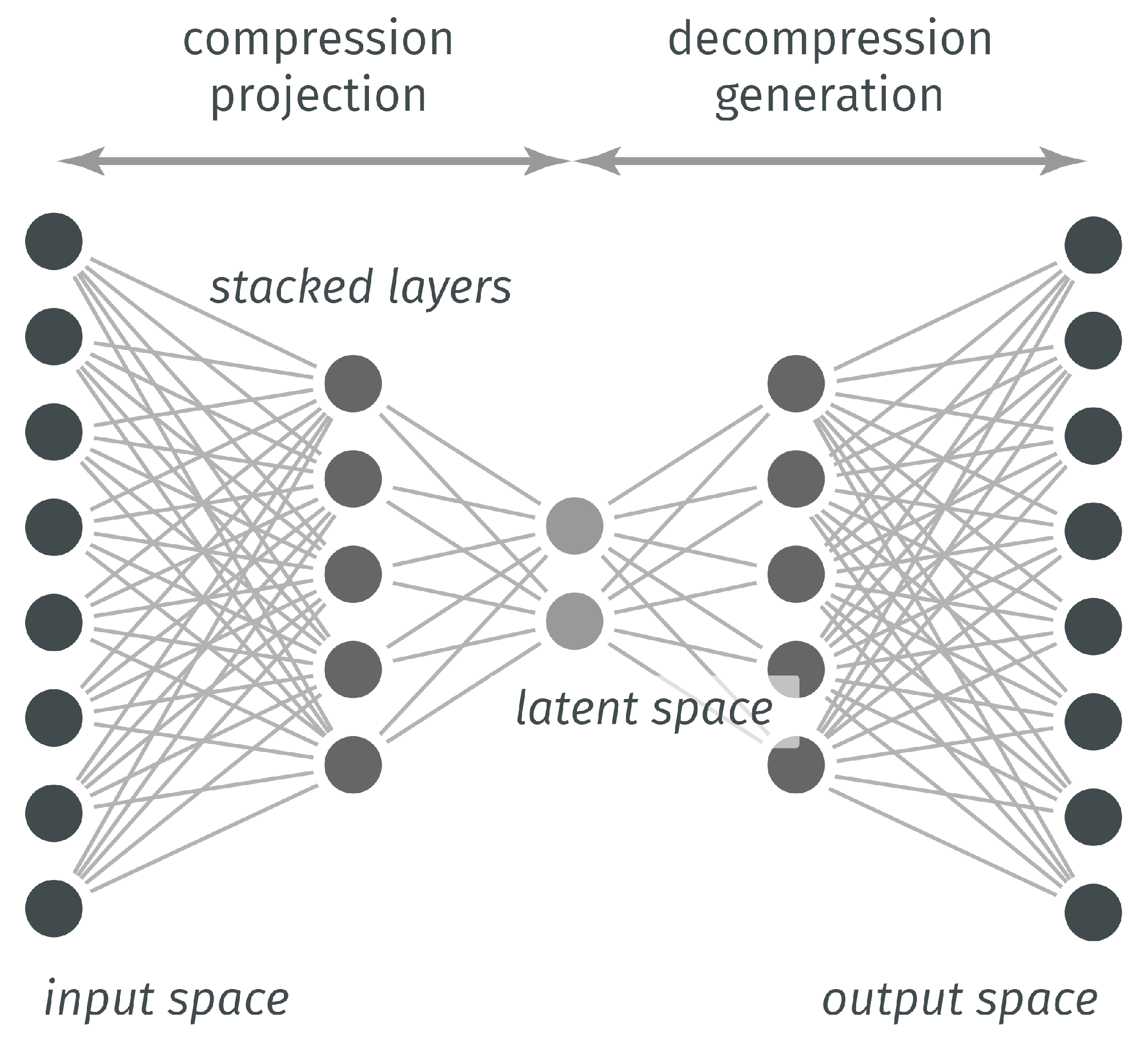
The FCAE used in this paper is a multi-layered neural network with an input layer, multiple hidden layers and an output layer (see
Figure 2). Each layer can have a different number of neural units and each unit in a layer is connected with every other one in the next layer. For this reason we call it here fully-connected, although in the literature it is usually refer to as autoencoder (AE), or to emphasise the multi-layer architecture aspect, as deep autoencoder (DAE) or stacked autoencoder (SAE). In all cases, an autoencoder performs two functions in a row: encoding and decoding.
The encoding function maps the input data to a hidden representation where and are respectively the weight matrix and the bias vector and is a non linear activation function such as the sigmoid or ReLU functions. The decoding function maps the hidden representation back to the original input space according to , being most of the time the same activation function.
The objective of the autoencoder model is to minimise the error of the reconstructed result:
where
is a loss function determined according to the input range, typically the mean squared error (MSE) loss:
where
u is the vector of observation,
v the reconstructed vector and
n the number of available samples indexed by variable
i.
The proposed FCAE architecture is described in
Table 2. We use three blocks of layers both in the encoder and decoder, which have a symmetric structure in terms of number of neural units per layer. The output shape refers to the shape of the tensors after the layers have been applied, where
,
and
refers respectively to the the batch size, (sliding) window length and number of features. The layer dimensions are defined as
,
and
.
The encoder Enc1 and Enc2 are blocks made up of pairs of Linear and ReLU activation layers. The input encodings (bottleneck with dimension ) are the result of Enc3. As a mirror of the encoder, the decoder has also two blocks (Dec1 and Dec2) both combining Linear and ReLU layers. The last decoding block (Dec3) is made up of a Linear layer with a Sigmoid activation as FCAE outputs are expected to be in the range of 0 to 1 (features are min-max scaled). A ReLU rather than a Sigmoid activation is used in all the other layers as it presents theoretical advantages such as sparsity and a minor likelihood of vanishing gradient resulting in faster learning.
5.2. Convolutional Autoencoder (CAE)
Table 3 shows the CAE architecture proposed in this paper. It is inspired from the one in [
23], which has been applied with good results for anomaly detection in time series data. The proposed CAE is a variant of the FCAE where fully-connected and convolutional layers are mixed in the encoder and decoder. Like the FCAE, the decoder structure is kind of a mirrored version of the encoder.
Table 3 shows also the shape of the input and output tensors in each layer, where
and
refers to batch size and number of features respectively. The input is three-dimensional, where the last dimension is the (sliding) window size (30) and the second dimension is the number of channels which in our case are the features (
). Unlike a FCAE, a change in the size of the input window may involve substantial parameter adaptation, because of the symmetric structure of the autoencoder and the nature of convolutional layers.
The first three layers of the encoder (
Conv1 to
Conv3) and the last three ones of the decoder (
ConvTransp1 to
ConvTransp3) are convolutional, whereas the innermost layers are fully-connected.
Conv1d(ic, oc, k, s, p) (and its transpose
Conv1DTransp(ic, oc, k, s, p, op)) denotes a convolutional (deconvolutional) layer with
and
channels, kernel size
k, stride
s and padding
p and output padding
. Please note that dimensionality reduction is achieved by using a
rather than by using pooling layers [
35].
All convolutional layers are followed by
BatchNorm layers [
36] to normalise the inputs to the activation layers.
ReLU is used as the activation layer everywhere except for the last one in the decoder (
ConvTransp3) where a
Sigmoid has been used instead for the same reasons stated with the FCAE.
We tested other alternative options for the activation functions, such as using
SELU everywhere (with appropriate LeCun normal initialisation of weights), or
Sigmoid in the dense layers and
ReLU in the convolutional ones as in [
23]. However, the results were worse and these options were abandoned.
5.3. LSTM Autoencoder (LSTMAE)
The blocks of the two autoencoders previously introduced are made up of either dense or convolutional layers, which makes necessary the use of sliding windows to provide them with fixed-sized input vectors. In this subsection, we introduce the LSTM autoencoders (LSTMAE), where layers consist of Long Short-Term Memory (LSTM) neural networks allowing for input sequences to be of variable length.
A LSTM is a type of RNN widely used for sequential data processing, since it can learn temporal dependencies over longer sequences than a simple RNN. For our particular purpose, a LSTMAE presents a theoretical advantage: samples can be entire flights instead of sliding windows, and anomaly scores can be calculated for the flight as a whole rather than by aggregating window anomaly scores.
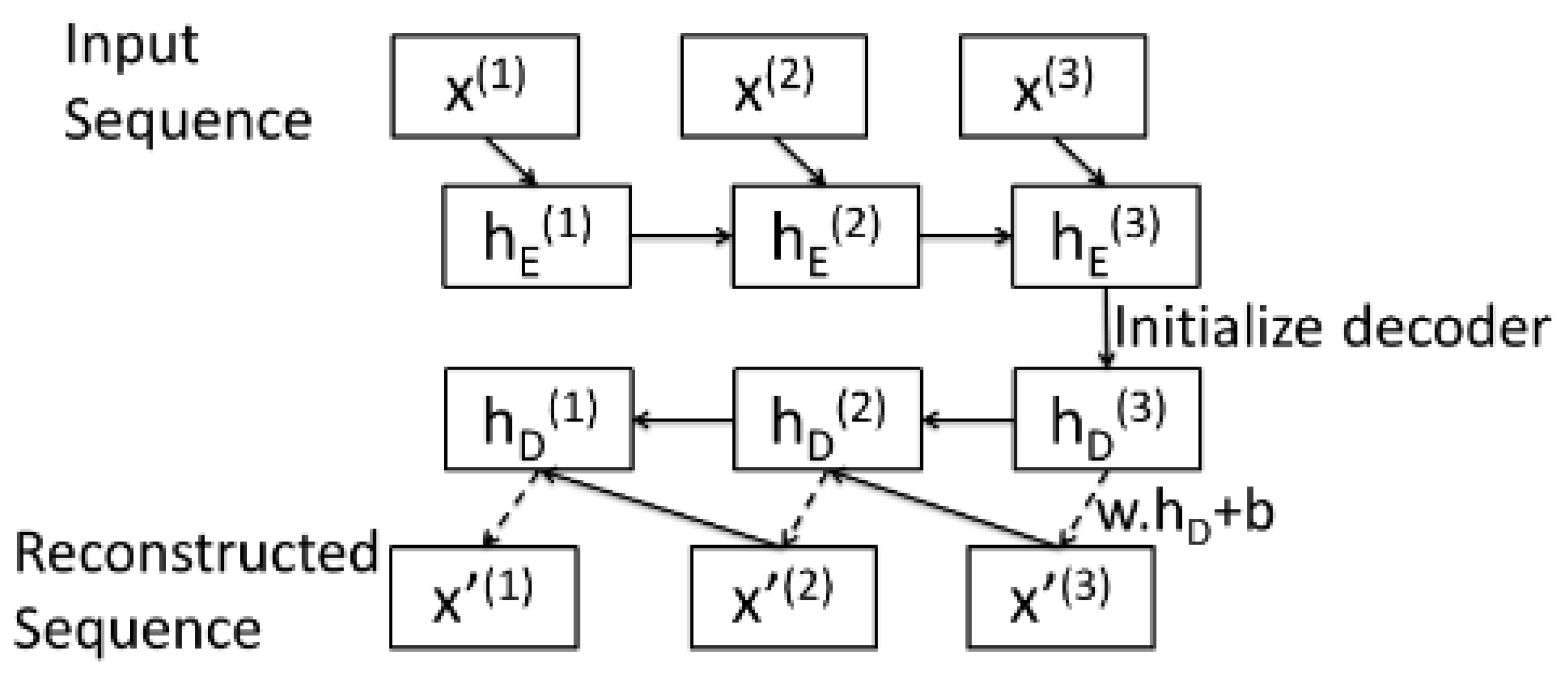
In the literature, there have been a few efforts to implement a LSTMAE. For instance, Malhotra et al. [
37] introduced the model in
Figure 3 for anomaly detection in time series data.
In this architecture, the encoder and the decoder are both LSTM networks. The last hidden state of the encoder is passed as the initial hidden state to the decoder. Then, at every instant t, the decoder takes as input the reconstruction of the previous instant obtained by linear transformation of the hidden state computed by the decoder cell.
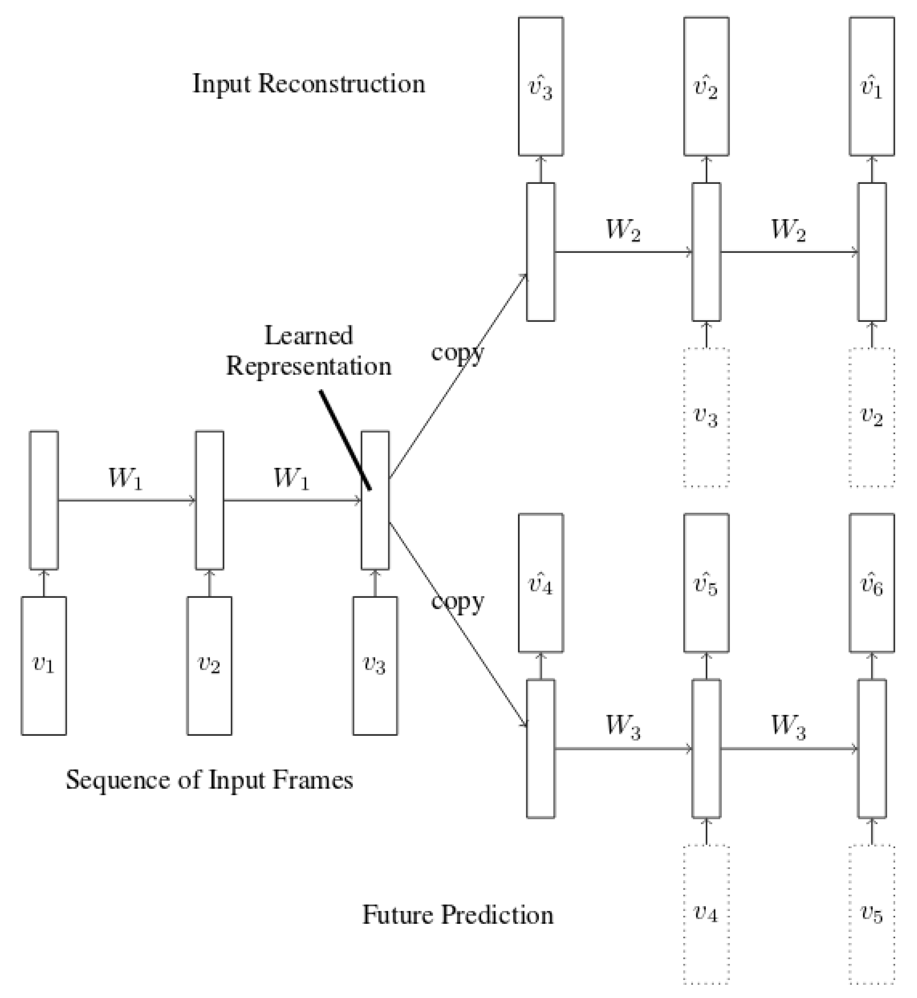
Srivastava et al. [
38] introduced the LSTMAE architecture shown in
Figure 4, which combines input reconstruction with future prediction in order to achieve a better hidden representation. Reconstruction is operated in reversed order as the last hidden state of the input sequence contains better information about the short-term correlations which should improve the reconstruction of the beginning of the sequence in reversed order.
The authors reported good results in both papers. However, Malhotra’s LSTMAE is mostly applied to short univariate time series of around 30 points, or several hundred points in the case of periodic series. As for Srivastava’s, good results are also reported with short video sequences (although of very high dimensions) by using high-dimensional hidden state vectors of size 2048 or even 4096.
We tested both LSTMAE architectures with our data and reconstructions were in general of poor quality, even with large latent spaces and after dimensionality reduction with severe signal downsampling and PCA. The intuition is these methods do not scale well when applied to our time series, which can reach several thousand points in long-haul flights. This could be explained by the fact that the hidden representation has not enough capacity to allow for a good reconstruction of a long and multivariate input sequence.
Pereira et al. [
39] mentioned this issue with long sequences and propose an attention-based mechanism to help the decoder. The resulting architecture is however highly complex, so we decided instead to work on a variant of the LSTMAE architectures by Malhotra and Srivastava. The goal is to test whether such an architecture could be good enough for our data when combined with appropriate dimensionality reduction.
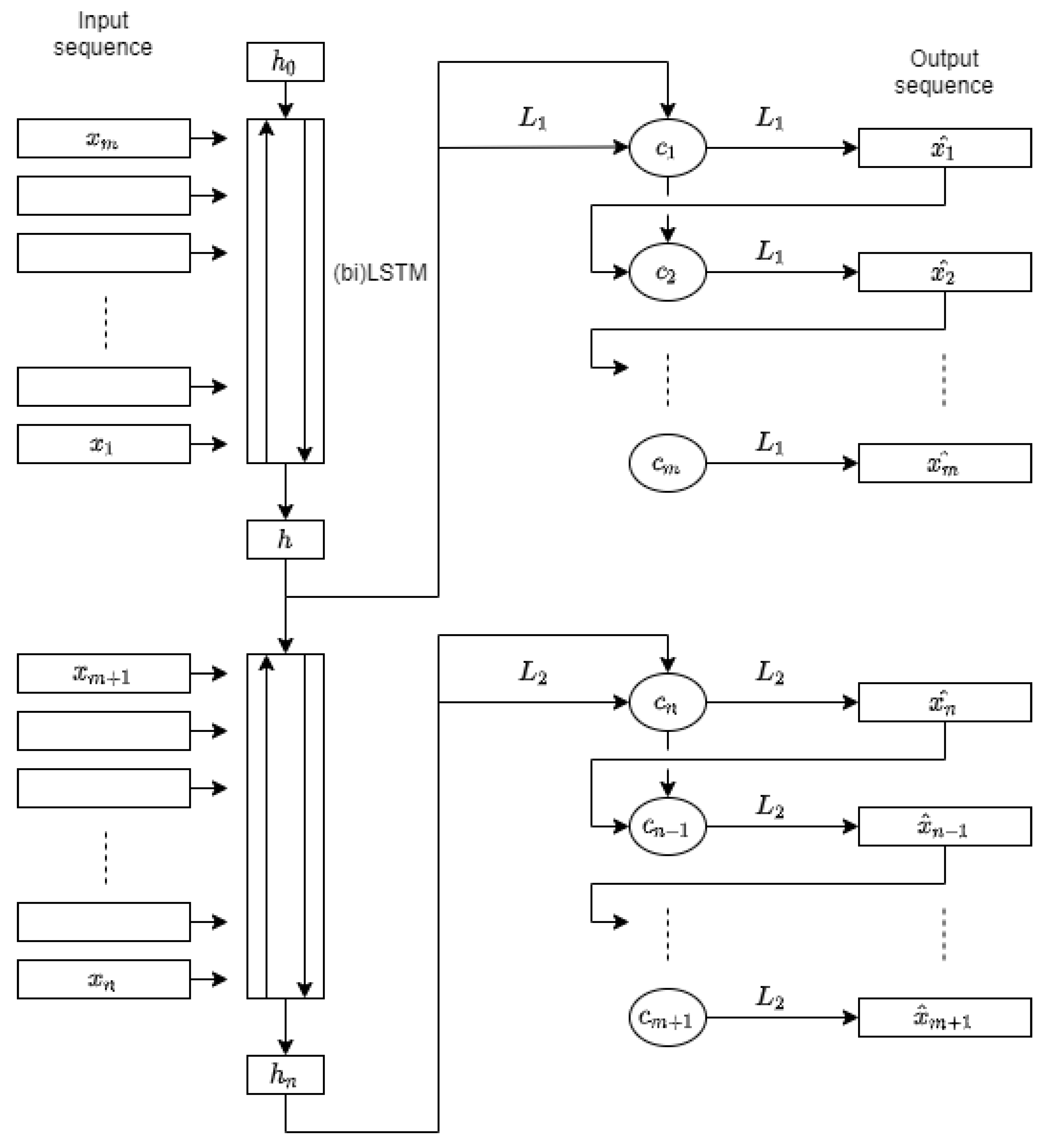
The proposed LSTMAE architecture is depicted in
Figure 5. Two encoders and two decoders are introduced to improve the reconstruction of long sequences, in particular the beginning and the end of the input sequence, where signal variation is very significant.
The input sequence of length
n is split in half, where each
(
) is a vector of size
(the number of features). In
Figure 5, each encoder is represented by a rectangular block of multiple LSTM cells, where
h and
are the last hidden state vectors output respectively by the top and bottom encoder. As for the decoders, they are both represented on the right side. The two sequences of small circles are the LSTM cells of the decoders. Each
outputs a hidden state vector computed from the reconstruction and the hidden state of the previous decoder step. The dimensions of all hidden states of the two encoders and decoders have been set to 80.
The top LSTM encoder receives the first half of the input in reversed order and computes latent representation h which is fed to the top decoder. The bottom encoder receives h and the second half of the input sequence in the original order and outputs the hidden representation . The top decoder takes h and linear transformation to feed cell state . The rest of the cell states () hidden states are computed from previous hidden state and reconstruction . The first half of the output sequence is obtained by linear transformation of the cell hidden states.
The inputs of the bottom LSTM encoder block are h and the second half of the input sequence in the original order, and its output the hidden state . The bottom decoder decodes the sequence in reversed order, and takes as inputs and linear transformation to output hidden state. The rest of the cell hidden states for () are computed from hidden state and . The second half of the output sequence is obtained by linear transformation of the cell hidden states and needs to be reversed.


