1. Introduction
Particle image velocimetry (PIV), a non-contact and transient velocity measurement method, was developed in 1980s [
1]. Since it was proposed, the technology has been developed rapidly and used widely [
2,
3,
4,
5,
6,
7]. The PIV system is mainly composed of a particle generator, a laser sheet optical system, a particle image acquisition system, and an image processing software. It works as follows. First, the particle generator is used to distribute tracer particles in the flow field. Then, the laser sheet optical system is used to output sheet light in a very short time to illuminate the measurement area of the flow field. At the same time, particle images are collected by the particle image acquisition system. Finally, the particle image is calculated by image processing software to obtain the velocity distribution of the measured area.
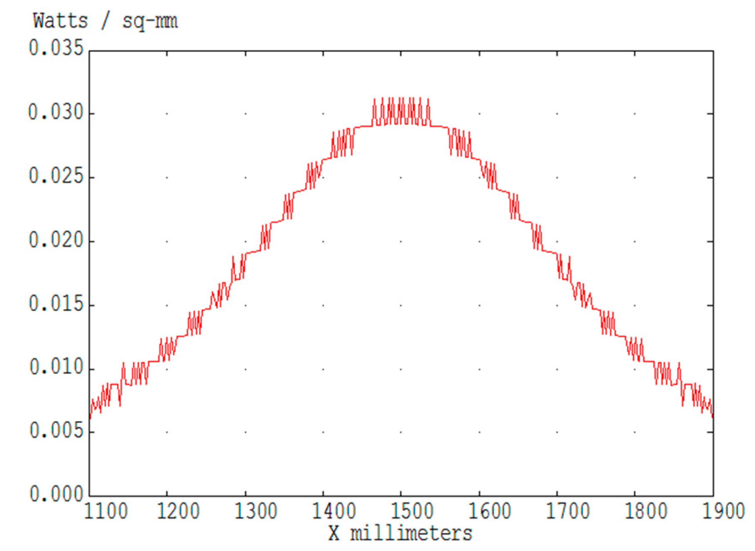
Laser sheet optical system is one of the key equipment of PIV, and it is an important guarantee to obtain high definition particle image. The most common optical system for extending a laser beam to a sheet light is the cylindrical lens group. The incident laser will be expanded into a linear laser when passing through two orthogonal concave and convex cylindrical lenses. This method is mature in technology and simple in structure. But in the case of large view field measurements, the sheet light uniformity is very poor. A simulation is conducted using ASAP software from Institute of Optics and Electronics. A laser beam with a diameter of 9 mm and divergence angle of 0.6 mrad is shaped into a sheet light of 800 mm × 1 mm by a cylindrical lens group after a distance of transmission. The light intensity distribution is shown in
Figure 1. The light intensity of the edge is only about 20% of the light intensity of the center. The image quality in the whole view field can be seriously affected.
Besides, Powell lens is also a common optical device to expand the laser beam into a sheet light [
8]. Its top is designed as a complex two-dimensional aspheric surface, and a large number of spherical aberrations are introduced to redistribute the optical path to form a linear laser. Although the sheet light uniformity of the Powell lens is improved compared with that of the cylindrical lens group, there is still a lot of room for improvement. In addition, the Powell lens is very sensitive to the matching of the incident laser and the aspheric surface of the lens.
The thickness of sheet light is also required in PIV experiment. If the sheet light is too thin, some particles may appear in one image and then disappear in the other image in a short time. This will directly affect the calculation of the two particle images. If the sheet light is too thick, some particles will be defocused on the image plane. The unclear particle image also affects the calculation accuracy. As a result, the sheet light thickness of PIV is generally controlled at about 1 mm in the measurement area.
In order to solve the problem of illumination uniformity of large view field and take into account the requirements of sheet light thickness in PIV, in this paper, a PIV laser sheet optical system is developed to achieve high uniformity illumination based on the theory of physical optics. This optical system helps to obtain high-resolution particle images in the whole view field.
2. Basic Knowledge of the Laser Sheet Optical System
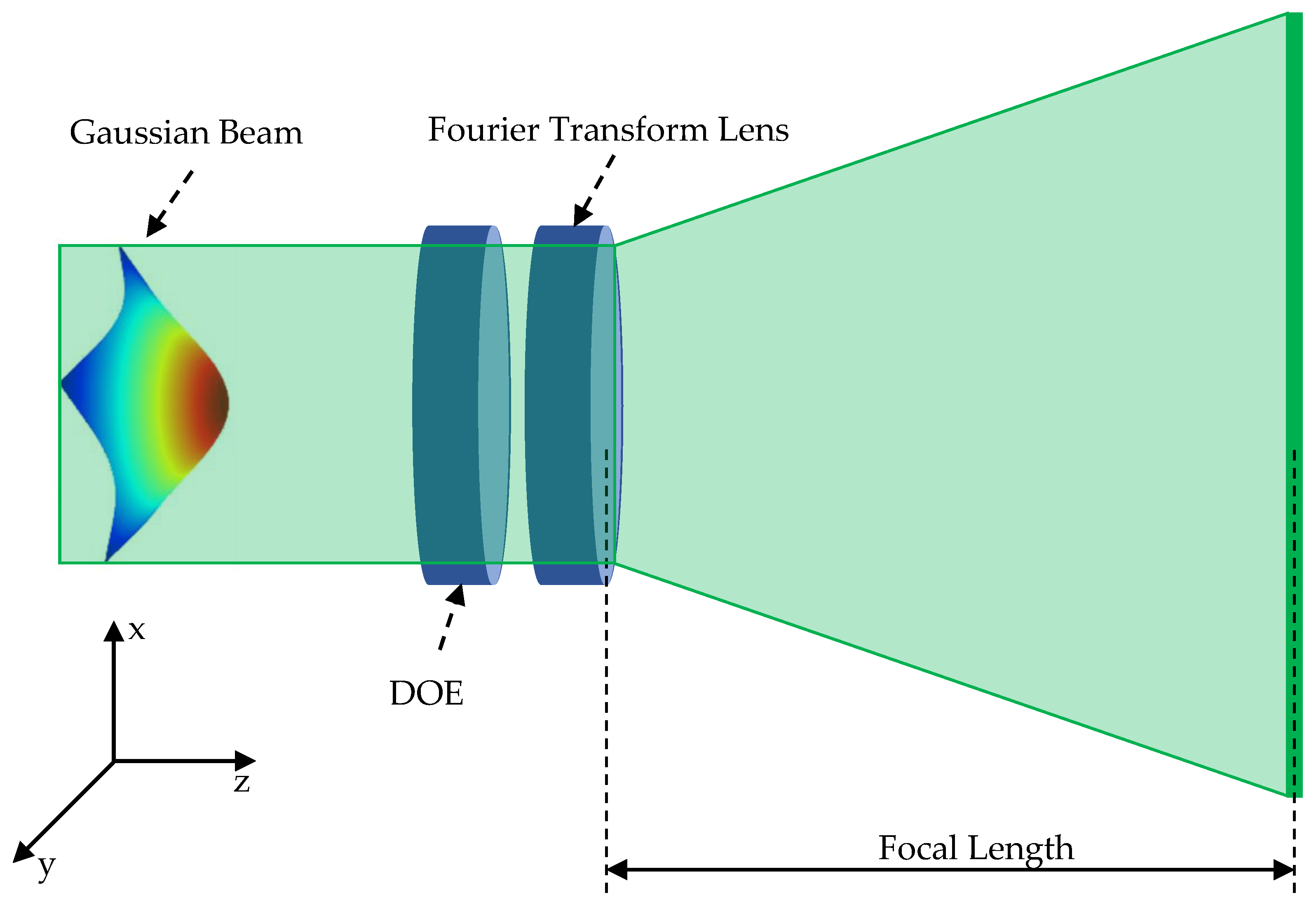
The laser sheet optical system can be regarded as a Fourier transform system based on Fraunhofer diffraction theory, as shown in
Figure 2. It is mainly composed of diffractive optical elements (DOE) and Fourier transform lens. The DOE has been widely used in coherent beam shaping because of light weight, small volume and good performance [
9,
10,
11]. It could realize some complicated illumination while other optical systems are hard to achieve good results.
The DOE is close to the Fourier transform lens. First, a collimated Gaussian beam is illuminated on the DOE. Then, the incident beam is phase modulated by the DOE and transformed by the Fourier transform lens. Finally, after some distance of transmission, the desired light intensity distribution is obtained on the image plane.
As the phase modulator in the system, the complex amplitude transmittance function of the DOE can be expressed as
According to Fraunhofer diffraction theory, if the complex amplitude distribution of the incident light field is
, the complex amplitude distribution of the output light field
can be expressed as
is the wavelength of light. f is the focal length of the Fourier transform lens.
. A constant phase factor
has been omitted from Formula (2), because it does not affect the light intensity distribution on the image plane.
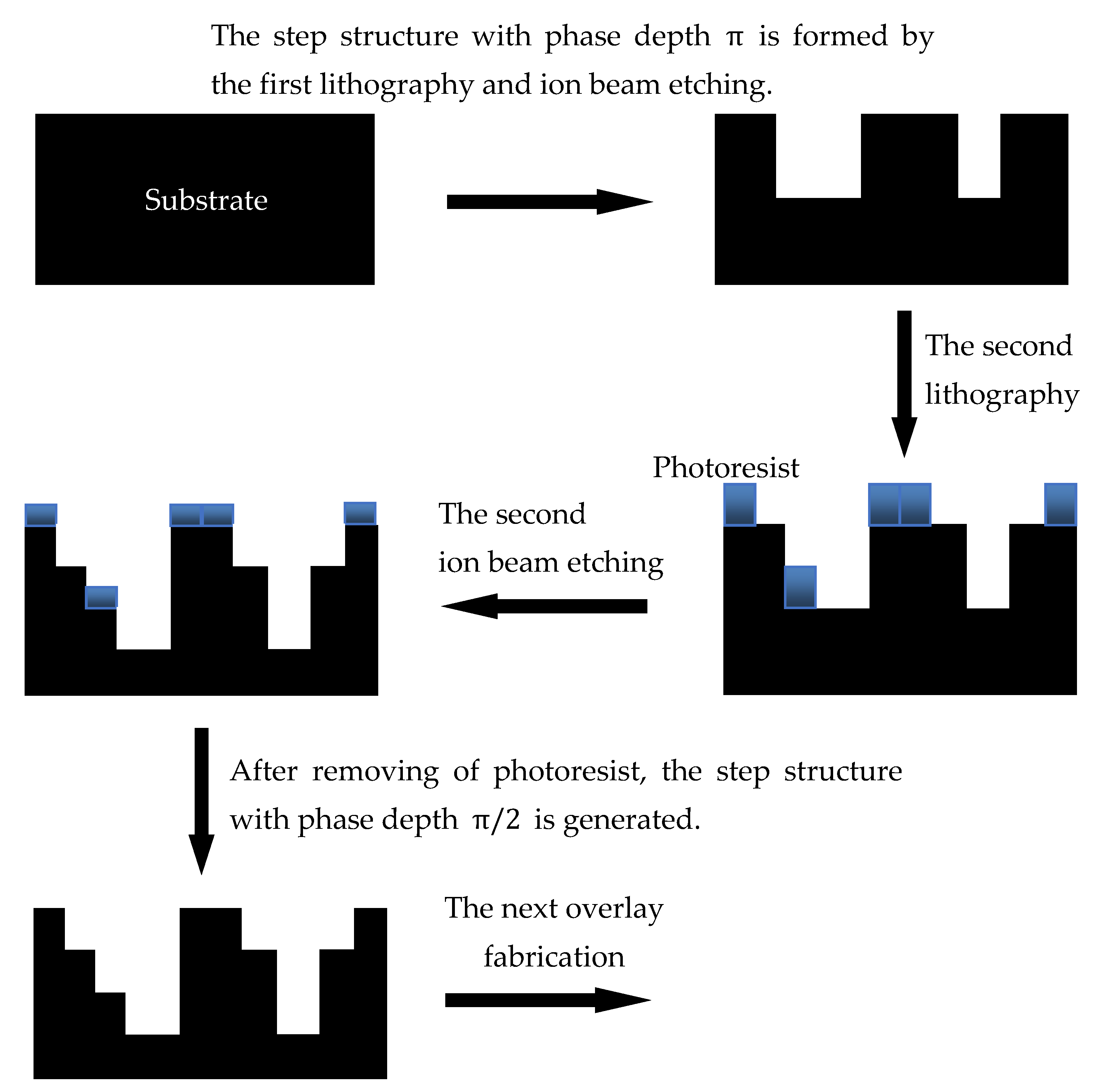
Further, the DOE is composed of millions of square tiny cells. The size of each cell is only a few microns. The depth of the tiny cells are precisely quantified and made by multiple lithography and ion beam etching. The schematic diagram of the fabrication process is shown in
Figure 3. After many times of overlay fabricate, the surface of the material can form a multi-step structure.
It can be seen from the fabrication process in
Figure 3 that 2
N steps can be obtained after N times overlay fabrication. The multi-step structure with phase depth
is generated in the first fabrication. The multi-step structure with phase depth
is generated in the second fabrication. The multi-step structure with phase depth
is generated in the third fabrication. So on, the multi-step structure with phase depth
will be generated in the N th fabrication. For example, a DOE with 8 steps can be obtained through 3 times overlay fabrication, and the phase depths are 0,
,
,
,
,
,
and
, respectively. The range of phase depth is
, and the relationship between substrate depth d and phase depth
can be expressed as
:
is the wavelength of light. n is the refractive index of the substrate material.
According to the basic theory of physical optics, when the optical paths of two beams differ by one wavelength , the phase difference is . Equation (3) can be deformed into . The incident collimating laser beam has an equal-phase wave front. From the perspective of micron scale, when the light beam passes through DOE, there will be optical path difference of the output beam at different positions because of DOE different step depth. As a result, the precise phase distribution of the light field can be achieved through these micro cells.
3. Design Algorithm of DOE
In order to evaluate the performance of DOE, two parameters are commonly used. The diffraction efficiency η is expressed as Equation (4). It represents the energy transformation efficiency. The higher the diffraction efficiency, the better the performance of DOE. The non-uniformity σ is expressed as Equation (5). It represents the uniform degree of intensity in target region. The smaller the non-uniformity, the better the performance of DOE.
D is the target region of the output beam.
is the intensity distribution on the output plane.
and
are the size of each cell on the output plane.
is the average intensity value of the output beam in target region. N is the number of sampling points in the target region.
In the optimization process, the two parameters need to be considered comprehensively. The definition of evaluation function is shown in Equation (6).
C is the regulation factor, which controls the relative ratio between the two parameters.
is the design value of diffraction efficiency. It can be seen that the smaller the evaluation function, the higher the diffraction efficiency and the better the uniformity of the laser sheet optical system.
In the design of DOE, the complex amplitude distribution of input light field and the complex amplitude distribution of output light field are known. In order to satisfy Formula (2), the goal is to solve the phase distribution . There are two types of algorithms commonly used.
The first is the iterative algorithm based on the Fourier transform or some other linear transform [
12,
13]. In 1972, before the concept of DOE was proposed, Gerchberg and Saxton proposed the iterative Fourier transform algorithm, the so-called G-S algorithm. Many of the improved algorithms that emerged later came from their algorithm. The algorithm first selects an initial phase distribution, then iterates repeatedly between the input and output light fields, and modifies the phase distribution with the ideal complex amplitude until the number of iteration reaches the set value or the objective function meets the set condition. G-S algorithm is simple in programming and fast in convergence, which is the most basic algorithm in DOE design. However, the G-S algorithm is very dependent on the selection of initial value, and the convergence process would stagnate. This means that the algorithm can only obtain local optimal solution.
The second is the global optimization algorithm based on extremum seeking [
14,
15,
16], such as simulated annealing algorithm, genetic algorithm, neural network algorithm, and so on. Genetic algorithm and neural network algorithm are mainly used in parallel computing environment. The computing efficiency of single computer is very low. The simulated annealing algorithm is mainly introduced here. This algorithm was proposed by Kirkpatrick in 1983. The idea of the algorithm comes from the annealing process of solid matter in physics. Starting from a higher initial temperature, the simulated annealing algorithm randomly searches for the global optimal solution of the objective function in the solution space with the continuous decrease of temperature. It can accept the deteriorative solution according to the probability and escape from the local optimal solution to the global optimal solution. However, the annealing process must be cooled slowly and the convergence rate of the algorithm is slow.
Therefore, after studying the above algorithms, a hybrid algorithm is proposed [
17]. It combines the iterative algorithm with the simulated annealing algorithm, which not only has the global optimization ability, but also greatly improves computational efficiency.
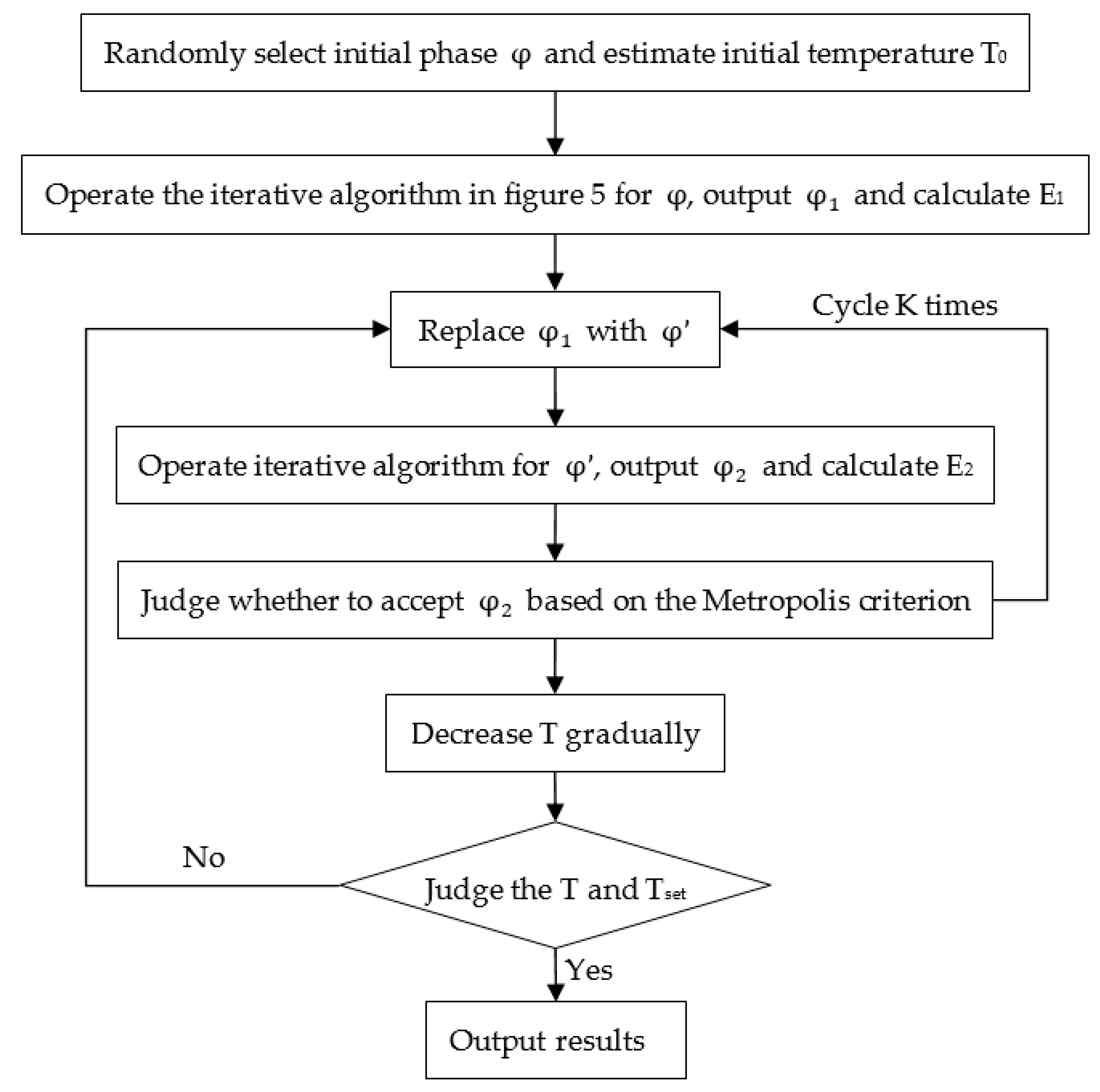
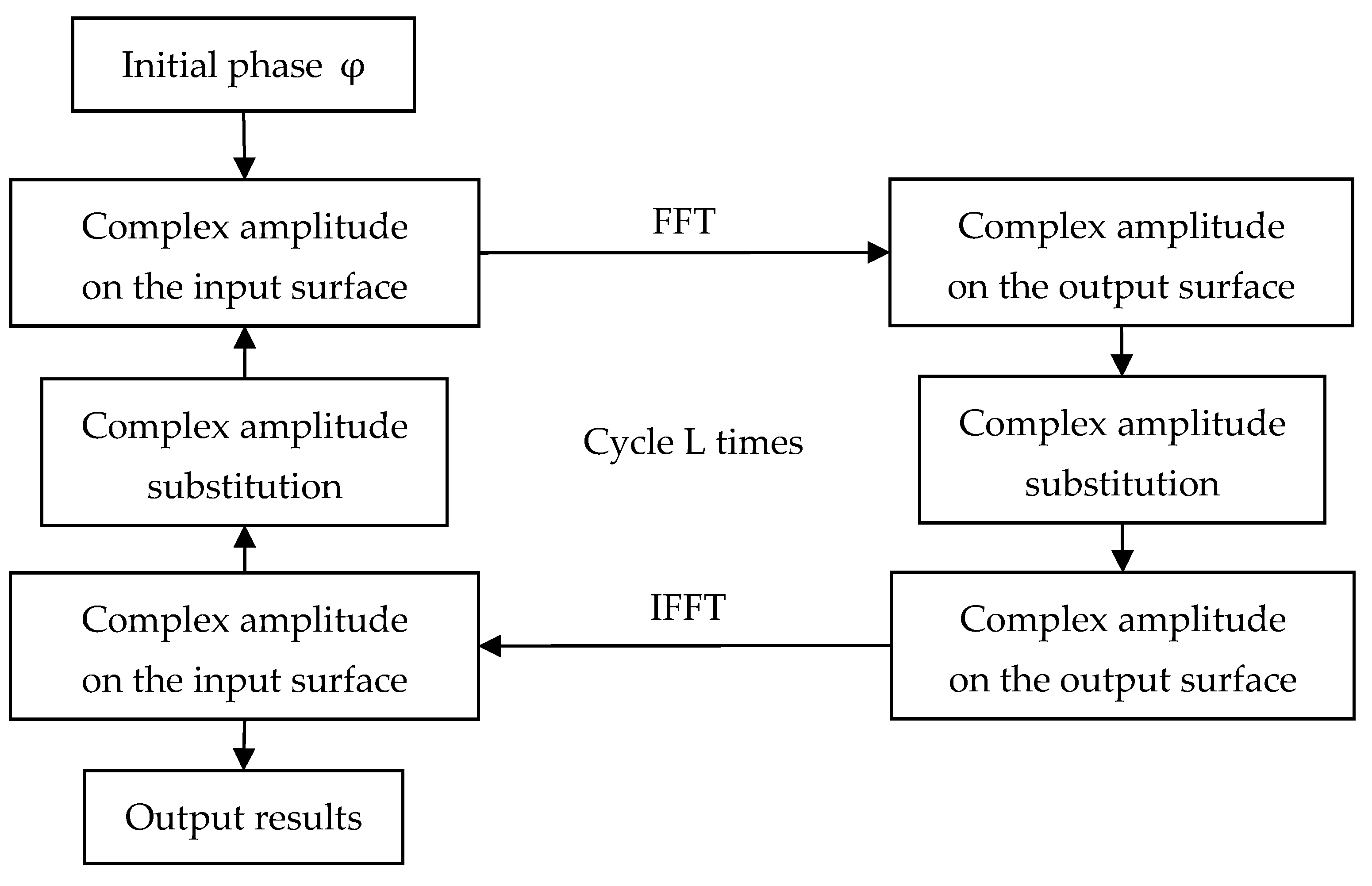
Figure 4 is the overall flow chart of the hybrid algorithm, and the detail steps are proposed as follows:
Randomly select the initial phase distribution and estimate the initial temperature of the optimization system. According to Metropolis criterion, . The initial acceptance probability . . is the evaluation function value in the initial state. is the evaluation function value which is calculated once by the hybrid algorithm. is the average of K cycles. Thus, the initial temperature is obtained.
Optimize the initial phase distribution with the iterative algorithm which is shown in
Figure 5. After this calculation, a local optimal solution
and its evaluation function
can be found.
Change the phase distribution
as follow:
is a random function, and
.
is a variable, and
. β will gradually decrease as the temperature T of the optimization system decreases.
Then make
as initial phase distribution for iteration (see
Figure 5) and calculate another local optimal solution
and its evaluation function
.
If , accept , and replace with If , calculate , if P is greater than or equal to some random number between 0 and 1, accept , and replace with , otherwise, refuse . This step allows the search process to change from a better solution to a worse solution with a certain probability to avoid the trap of local optimization. This is the biggest difference between global optimization algorithm and local optimization algorithm.
Go to step 3. In order to reach thermal equilibrium at temperature T, the number of cycles should be more than 50 times.
Decrease T gradually. If the system temperature is higher than the minimum temperature , go back to step 3 to continue the calculation. If the temperature T is less than the minimum temperature , this program should be ended and output final phase distribution.
This hybrid algorithm combines the advantages of simulated annealing algorithm and iterative algorithm. It not only has fast convergence speed, but also has the ability of global optimization. Besides, the algorithm is simple to operate. The initial phase distribution is selected randomly, and the calculation process does not need manual intervention.
4. Design Results
A DOE is designed for laser sheet optical system of the PIV. The parameters are shown in
Table 1.
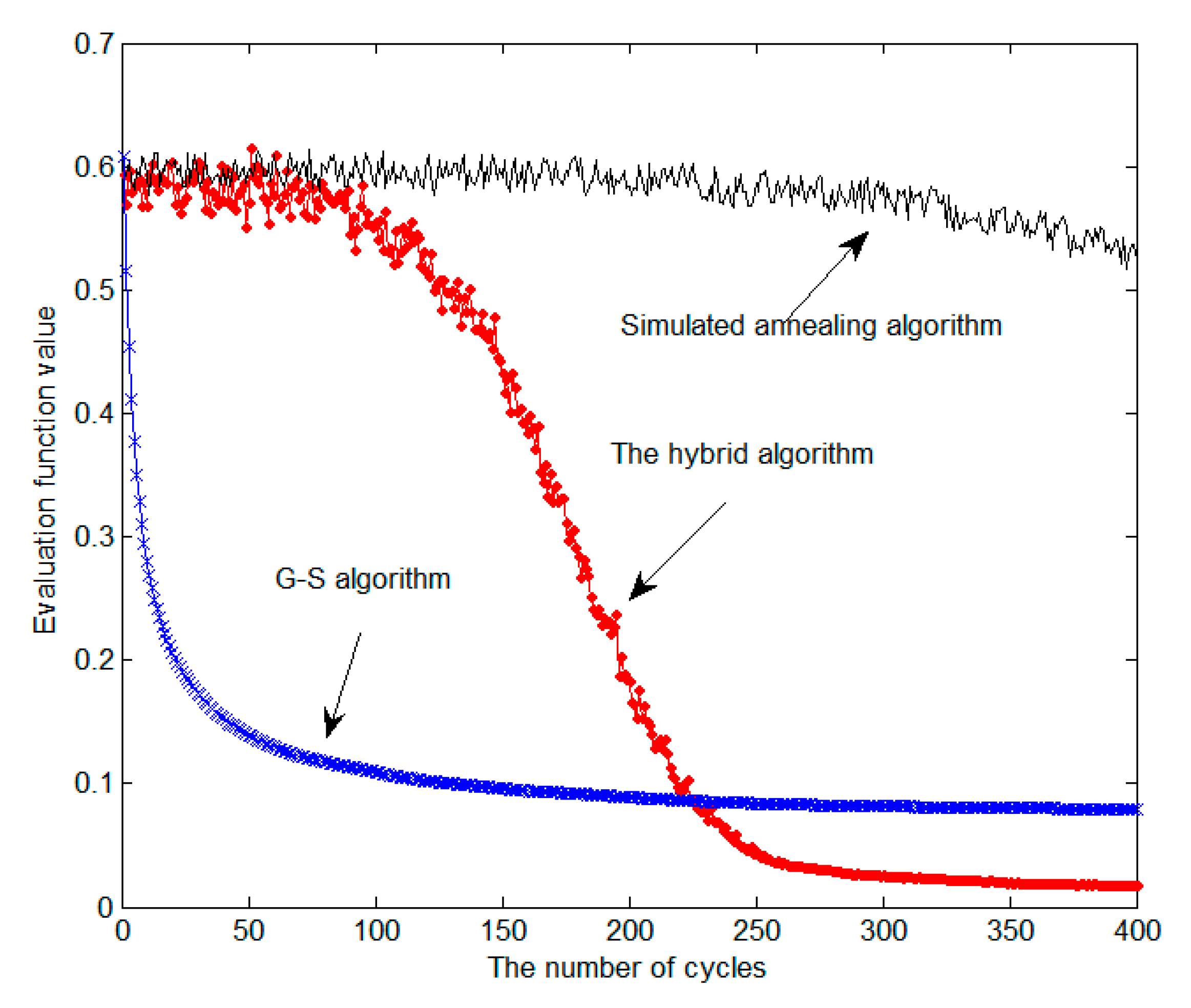
The hybrid algorithm is compared with the simulated annealing algorithm and G-S algorithm in
Figure 6. The initial phase distribution is the same for comparison purposes. According to Equation (6), it is easy to know that the smaller value of the evaluation function, the better beam shaping effect. As shown in
Figure 6, the convergence property of simulated annealing algorithm decreases slowly with the increasing cycles. However, the convergence property of G-S algorithm decreases too fast to stagnate. The convergence property of the hybrid algorithm is obviously better.
Table 2 shows the comparison of the design results of three algorithms.
in Equation (6). The design results also show that the hybrid algorithm is obviously better than the other two algorithms.
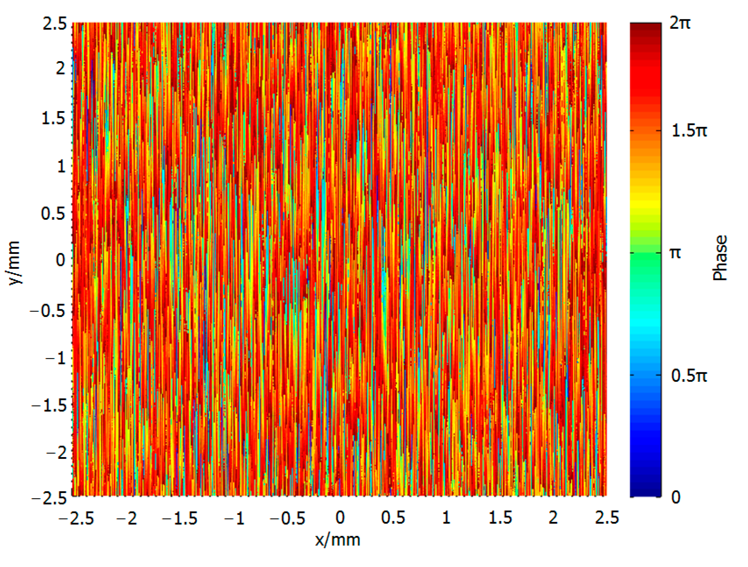
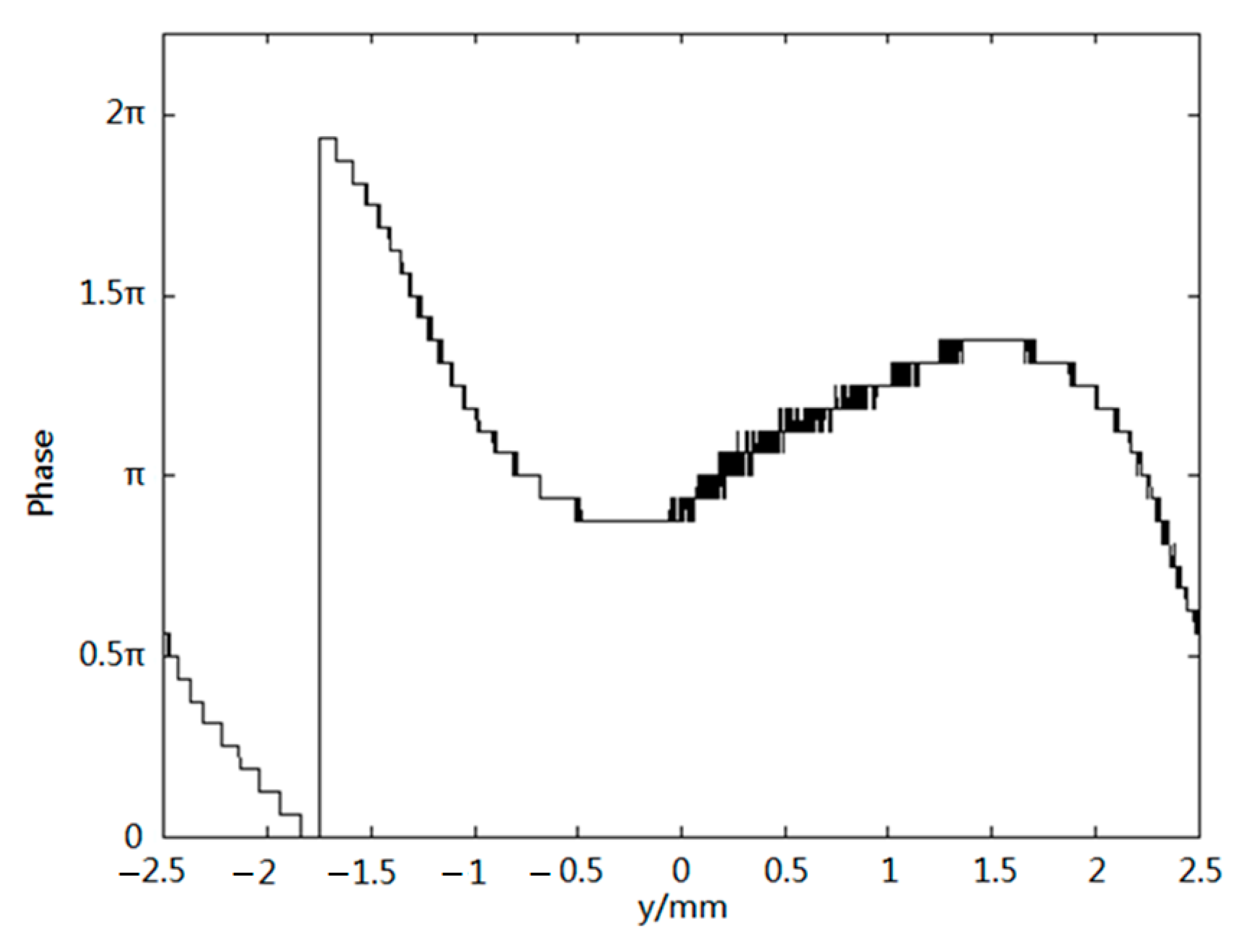
The phase distribution of the DOE, which is designed by the hybrid algorithm, is shown in
Figure 7. DOE is composed of 4 million square tiny cells. The size of each cell is
. Each micro cell has a definite phase value
through hybrid algorithm optimization. Precise phase modulation can be achieved at each point of the light field through these micro cells.
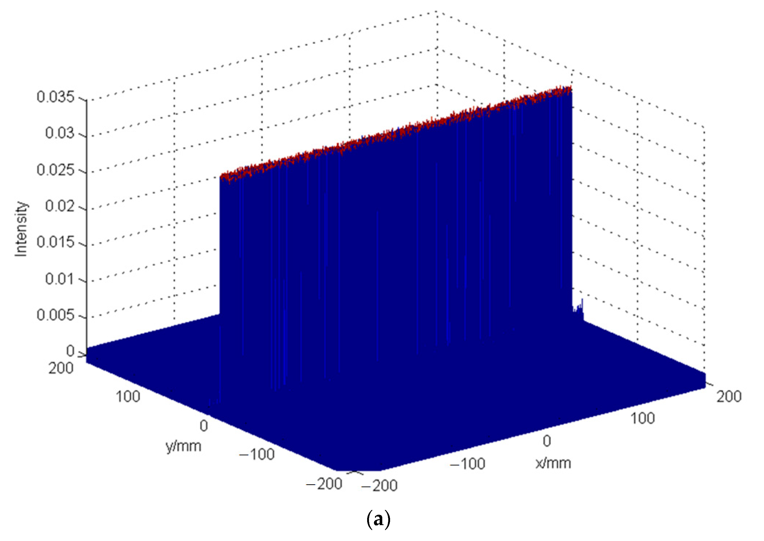
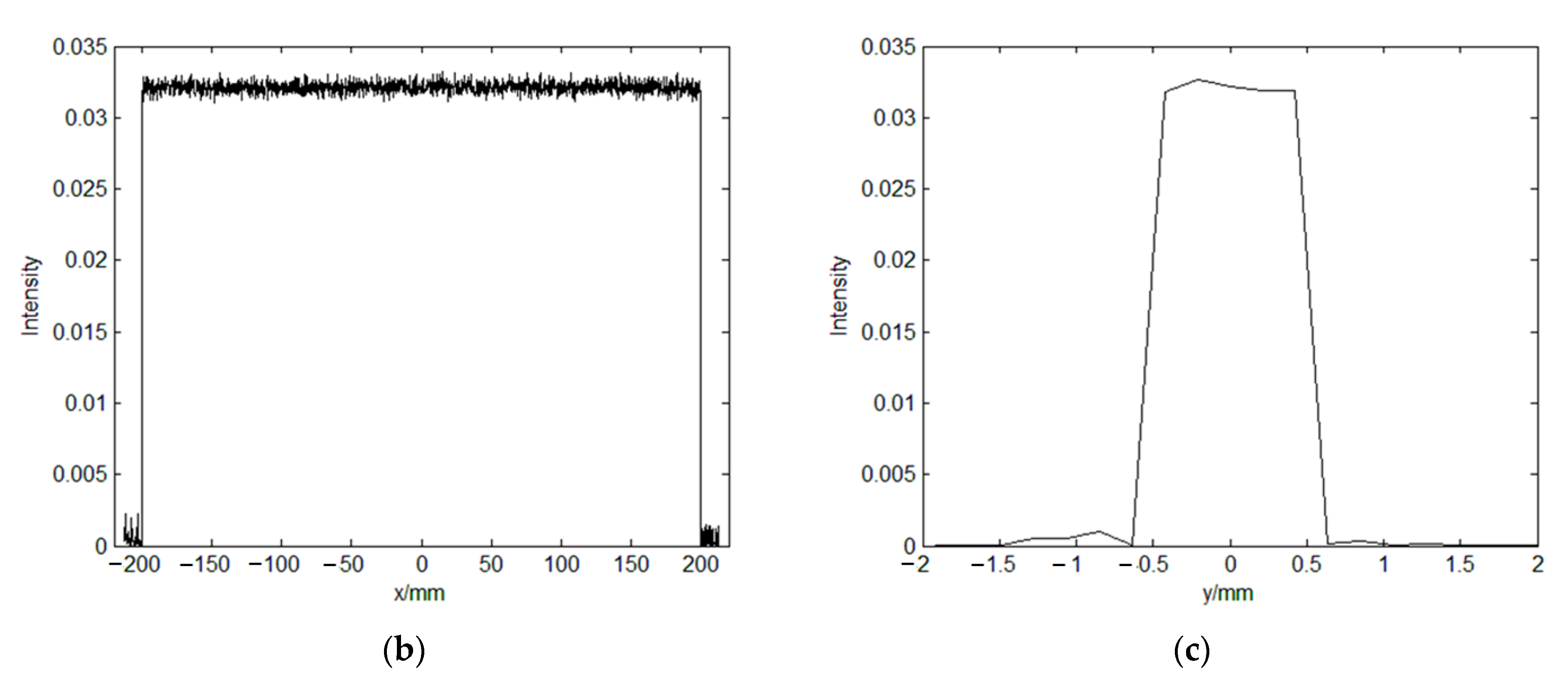
The intensity distribution of the sheet light is shown in
Figure 8. It is worth noting the value of the light intensity in
Figure 8. The energy in the input plane is equal to the energy in the output plane when energy loss is ignored during beam transmission.
is the input plane.
and
are the size of each cell on the input plane.
is the output plane.
and
are the size of each cell on the output plane. In addition, due to the limitation of the disperse Fourier transform, the relationship between
,
and
,
can be expressed as [
17]:
M = 2000 is the total number of sampling points in a single direction. Z is the distance between the input plane and the output plane.
During the calculation, the maximum relative intensity of the incident Gaussian beam is assumed to be 1, and the restriction conditions of energy conservation and disperse Fourier transform are strictly observed. Thus, the light intensity values shown in
Figure 8 are obtained. In addition, from the description of the design process in
Section 3, the DOE phase distribution is randomly generated. Some conditions are specified to judge whether to accept this randomly generated DOE phase distribution with the ideal sheet light as the optimization target. So, the light intensity distribution on the image plane fluctuates around the design value, which looks like random noise.
As can be seen from the
Figure 8, the width of the sheet light in the image plane is 400 mm, and the thickness of the sheet light in the image plane is 1 mm. The diffraction efficiency reaches 97.77% and the non-uniformity is only 0.03%. As a result, the hybrid algorithm described in
Section 3 can obtain excellent design results.
According to the 2nd section, the more steps are quantized, the closer the DOE surface shape is to the design shape, but the fabrication process will be more complicated. When the number of steps is 32, the DOE needs 5 times overlay fabrication. The phase values go from 0 to
in increments of
. The diffraction efficiency and non-uniformity of the sheet light approach the design value, and the fabrication difficulty is acceptable. Its performance is suitable for PIV experiments. Therefore, the DOE is quantified into 32 steps, as shown in
Figure 9.
5. Analysis of the Sheet Light Quality in Measurement Area
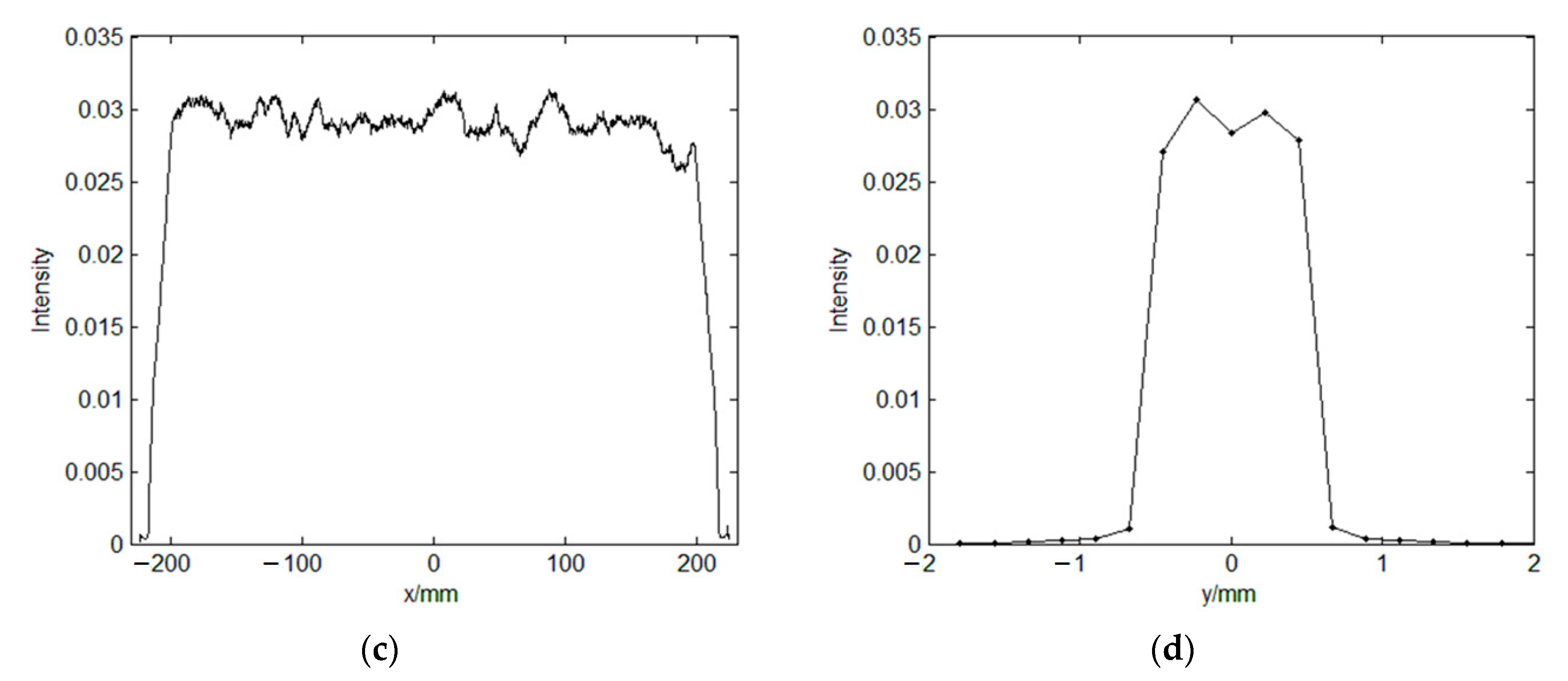
In the PIV experiment, the thickness of the sheet light should be controlled at about 1 mm in the whole measurement area, and the diffraction efficiency and uniformity of the sheet light should also be guaranteed. Fresnel diffraction Formula (10) can be used to calculate the light intensity distribution at
position.
In the formula, is the phase transformation factor of the Fourier transform lens. When , Formula (10) becomes Formula (2).
and
are selected to simulate from the DOE design results of
Section 4, and the intensity distribution of the sheet light is shown in
Figure 10.
At
, the width of the sheet light is about 385 mm, the thickness of the sheet light is about 0.9 mm, the diffraction efficiency is 95.98%, and the non-uniformity is 0.44%. At
, the width of the sheet light is about 418 mm, the thickness of the sheet light is about 1.1 mm, the diffraction efficiency is 96.21%, and the non-uniformity is 0.35%. As a result, the thickness of the sheet light can be controlled at about 1 mm in the 200 mm depth measurement area. Although the diffraction efficiency and uniformity of the sheet light are affected by defocus, the optical system can still satisfy the requirements of PIV experiment. In addition, the size of the sheet light would scale equally with the change of Z value. The main reason is the size of
and
have changed, which can be explained by Equation (9). Meanwhile, by combining Equations (8) and (9), it can be deduced that:
Only Z is the independent variable in the above equation. It can be seen that the value of light intensity on the output plane would also vary with the change of Z value.
6. Conclusions
In this paper, a high uniformity laser sheet optical system for PIV is designed based on physical optics theory. The optical system is mainly composed of DOE and Fourier transform lens, which has the advantages of simple structure and easy integration. The sheet light has extremely high uniformity. As a result, the optical system helps to obtain high-resolution particle images in the whole measurement area. In addition, the comparison with G-S algorithm and simulated annealing algorithm shows that the hybrid algorithm used in the DOE design has both fast convergence speed and global optimization capability. It can acquire excellent design results. This work also can be applied to a series of non-contact flow field measurement techniques such as plane laser induced fluorescence, filtered Rayleigh scattering, two-color plane laser-induced fluorescence temperature measurement, and high uniformity 3D illumination of tomographic PIV.
Author Contributions
Conceptualization, Y.K., Z.J., and C.S.; methodology, Y.K.; software, Y.K.; writing—original draft preparation, Y.K.; writing—review and editing, Z.J.; project administration, C.S. All authors have read and agreed to the published version of the manuscript.
Funding
This research was funded by National Natural Science Foundation of China, grant number 91641118.
Data Availability Statement
Data sharing is not applicable to this article.
Conflicts of Interest
The authors declare no conflict of interest.
References
- Adrian, R.J. Scattering particle characteristics and their effect on pulsed laser measurement of fluid flow: Speckle velocimetry vs. particle image velocimetry. Appl. Opt. 1984, 23, 1690–1691. [Google Scholar] [CrossRef] [PubMed]
- Dadi, M.; Stanislas, M.; Rodriguez, O.; Dyment, A. A study by holographic velocimetry of the behavior of free small particles in a flow. Exp. Fluids 1991, 10, 285–294. [Google Scholar] [CrossRef]
- Calluaud, D.; David, L. Stereoscopic particle image velocimetry measurements of the flow around a surface-mounted block. Exp. Fluids 2004, 36, 53–61. [Google Scholar] [CrossRef]
- Yu, J.; Wang, J.J.; Shi, L.L.; Liu, Y.Z. TR-PIV Measurement Technology Using Continuous Laser Illumination. J. Shanghai Jiaotong Univ. 2009, 43, 1254–1257. [Google Scholar]
- Jia, Y.; Jiang, N. Tomographic PIV experimental investigation of topological modes of modulated Reynolds stress and velocity strain rate for coherent structure. J. Exp. Fluid Mech. 2012, 26, 6–16. [Google Scholar]
- Gao, Q.; Wang, H. Tomo-PIV technology and its synthetic jet measurement. Chin. Sci. Tech. Sci. 2013, 7, 106–113. [Google Scholar]
- Hasler, D.; Landolt, A.; Obrist, D. Tomographic PIV behind a prosthetic heart valve. Exp. Fluids 2016, 57, 1–13. [Google Scholar] [CrossRef]
- Zhong, Q.; Chen, Q.; Wang, X.; Li, D. On the improvement of PIV light sheet quality. J. Exp. Mech. 2013, 28, 692–698. [Google Scholar]
- Kato, Y.; Mima, K.; Miyanaga, N.; Arinaga, S.; Kitagawa, Y.; Nakatsuka, M.; Yamanaka, A.C. Random phasing of lasers for uniform target acceleration and plasma instability suppression. Phys. Rev. Lett. 1984, 53, 1057–1060. [Google Scholar] [CrossRef]
- Turunen, J.; Paakkonen, P. Diffractive shaping of excimer laser beams. J. Mod. Opt. 2000, 47, 2467–2475. [Google Scholar] [CrossRef]
- Victor, B.Y.; Farson, D.F.; Ream, S.; Walters, C.T. Custom beam shaping for high power fiber laser welding. Weld. Res. 2011, 90, 113–120. [Google Scholar]
- Gerchberg, R.W.; Saxton, W.O. A practical algorithm for the determination of phase image and diffraction plane pictures. Optik 1972, 35, 237–246. [Google Scholar]
- Zhou, J.; Lu, Y.; Wang, L.; Cai, N.; Wang, X. An Improvement on GS Algorithm for Design of Computer Optical Elements. J. Optoelectron. Laser 2007, 18, 1180–1183. [Google Scholar]
- Kirkpatrik, S.; Gelatt, C.P.; Vecchi, M.P. Optimization by simulated annealing. Science 1983, 220, 2145–2158. [Google Scholar] [CrossRef] [PubMed]
- Bennett, A.P.; Shapiro, J.L. Analysis of genetic algorithms using statistical mechanics. Phys. Rev. Lett. 1994, 72, 1305–1309. [Google Scholar] [CrossRef] [PubMed]
- Li, J.L.; Zhu, S.F.; Lu, B.D. Design and optimization of phase plates for shaping partially coherent beams by adaptive genetic algorithms. Opt. Laser Technol. 2010, 42, 317–321. [Google Scholar] [CrossRef]
- Yin, K. Research on Stray Light in Diffractive Optical System. Ph.D. Thesis, University of Chinese Academy of Sciences, Beijing, China, 2014. [Google Scholar]
| Publisher’s Note: MDPI stays neutral with regard to jurisdictional claims in published maps and institutional affiliations. |
© 2021 by the authors. Licensee MDPI, Basel, Switzerland. This article is an open access article distributed under the terms and conditions of the Creative Commons Attribution (CC BY) license (https://creativecommons.org/licenses/by/4.0/).


