Winglet Geometry Impact on DLR-F4 Aerodynamics and an Analysis of a Hyperbolic Winglet Concept

Abstract

In this article, the growth of aerodynamic efficiency and the growth of the wing structural stress is studied for DLR-F4 typical transport aircraft wing-body, after installing classical Whitcomb winglets of different configurations and a delta wingtip fence. A new-concept curved-span winglet was mathematically developed and approved through Computational Fluid Dynamics (CFD) and static structural experiments, revealing the interaction of sub- and transonic air flow dynamics with the wingtip device geometry. The design space of the winglet geometry was explored briefly, and an evaluation of the lift-to-drag ratio increment depending on various winglet input parameters was performed. In particular, the winglet cant angle effect on lift and drag was thoroughly analyzed at various flow regimes and angles of attack, revealing an ambiguity and a conflicting character of results between highly canted winglets and nearly vertical ones. As a result of cant angle impact analysis, a curved winglet concept is suggested and mathematically parametrized, that could provide an innovative solution, alternative to a morphing winglet, but much simpler with a fixed structure. In conclusion, a multidisciplinary winglet efficiency estimation criterion is suggested for comparing the aerodynamic efficiency of different wingtip devices with respect to their structural weight penalty in real flight conditions.

1. Introduction

The potential advantage of using non-planar lifting surfaces to reduce induced drag has long been known. These include closed wings, C-wings and wings with winglets. Despite recent technological advances and the use of high rigidity Carbon Fiber Reinforced Plastic wing panels that allow very large aspect ratios, which greatly cut the induced drag at cruise, most airframe manufacturers are still applying winglets, both for further pushing the boundaries of the wing aerodynamic efficiency and due to their aesthetic value. Since their introduction in 1975 by National Aeronautics and Space Agency (NASA) engineer Richard Whitcomb [1,2], winglets have undergone major geometrical changes, driven by the quest for a sustainable efficiency throughout the entire flight envelope of modern airliners. Due to the largely different flow field nature at the wing tip area at different flight conditions, and the challenge of achieving a winglet shape optimal throughout the whole flight envelope, recent winglet geometry optimization studies in the last decade were mostly focused on cruise as a ‘design case’ for this wingtip device, resulting in trade-off solutions less optimal for take-off and climb at high angles of attack [3,4,5,6,7,8,9,10]. Few innovative solutions have been suggested including morphing winglets which adapt their cant and/or twist depending on the flow regime [11,12,13], or using an integrated moving device such as a winglet-integrated rudder [14,15] or a gust alleviating conventional aileron [16], as well as active vortex wake control with an oscillating mechanism [14,17,18]. Bio-inspired devices were studied with a triangular leading-edge extension [19], with multiple elements, where each element is set at a given angle and contributes at a certain flight regime, thus sustaining overall efficiency [20,21]. To date, none of these novel solutions could find application on an operational airliner, mainly due to their high complexity which both compromises reliability, and involves a weight penalty, potentially cancelling their aerodynamic gains.

Most winglet geometry optimization attempts [3,4,5,6,7,8,9,10] are purely experimental, based on the results of either computational and/or wind tunnel experiments on a large population of samples with a subsequent optimization using a statistical approach such as pareto front. Unfortunately, the general lack of a winglet local-flow-field theory makes it challenging to explain experimental results, and to uncover proper improvement directions for future designs. Keizo et al. [3] performed high fidelity CFD and wind tunnel multidisciplinary design exploration of a commercial jet winglet, which provides a fairly deep insight into the winglet design space, allowing an optimal design decision based on pareto front and simple trade studies. Although this is a pragmatic approach usually used by airframers to retrofit operational airliners with winglets [6,7], it results in an improved initial geometry, rather than a novel design, due to the lack of a closed-form relationship between the winglet geometry and overall lift-to-drag ratio. Given the winglet is a finite span lifting surface, classical wing theory has been extended to predict the winglet performance. For instance, a CFD combined with the lifting line theory approach has been used by Jan Himisch [4] and Streit et al. [6] to obtain an optimal cruise L/D ratio for a generic transonic airliner. An attempt of finding a winglet optimal twist was performed by Neal [10], by relating the winglet root and tip incidence angles with the induced drag reduction, obtained as output from potential flow solutions in the Trefftz plane behind the wing. However, there are virtually no recent theoretical or experimental studies of the winglet geometry impact on its local flow field and how this correlates with overall efficiency. Therefore, the current work is aimed at filling this gap through a quantitative analysis.

In this paper, a brief design space exploration of a wingtip fence and a classical winglet is presented and a detailed study has been performed on the winglet local flow field, where DLR-F4 lift and drag are correlated with changes in the winglet local angle of attack spanwise, which in turn changes according to the aircraft angle of attack and the winglet’s own geometrical parameters, in particular its cant angle. CFD and analytic search for an optimal cant angle has led to considering a spanwise-variable cant (curved) winglet concept, alternative to cant-morphing solutions presented in [11,12,13]. The curved winglet span was parametrized using a second order function, which was in turn optimized for getting the most beneficial local angle of attack distribution. Recently, the concept studied herein, of a curved-span winglet, has become relatively well-established with the introduction of blended winglets by Aviation Partners, Inc. [9,22], and Airbus wide body A350 XWB and very lately, the new long range A330 Neo, both featuring a double curvature (spanwise and plan form) winglet [23,24]. At the concluding part, a comparison of the static structural stress growth on the wing structure is given for each of the CFD-analyzed wingtip devices, allowing an overall evaluation of their weight penalty, and its juxtaposition to their aerodynamic benefits.

An important contribution of this paper is the front-view parametrization and optimization method used herein for a non-planar lifting surface, applying as an objective function the spanwise local angle of attack distribution. Whereas most parametrization studies for planar wings seek either an optimal plan form, optimal span-wise airfoil shape variation and/or chord-wise airfoil curvature variation (see [25] for instance), the front projection optimization issue is paramount for non-planar lifting surfaces as wings with winglets, c-wings and closed lifting surfaces, where both the geometric and effective local angles of attack do not change uniformly spanwise, when the aircraft angle of attack changes. Examples of other approaches for winglets parametrization can be found in [25,26]. The evolutionary geometry parametrization approach presented by Zingg et al. in [25] can be applied to parametrize a span-curved winglet geometry by starting from a classical straight winglet then using B-spline approximation to get a generic curved winglet, and by inserting additional knots at the winglet root and/or tip sections, based on gradual inclusion of different design variables. A comprehensive study by Luciano et al. [27] gives a method for predicting the minimum induced drag of non-planar wings through a configuration-invariant analytic formulation of the unknown circulation distribution. The authors present a numerical tool implementable in MATLAB, which allows the definition of non-planar wings’ optimal circulation distribution with minimum induced drag.

2. Materials and Methods

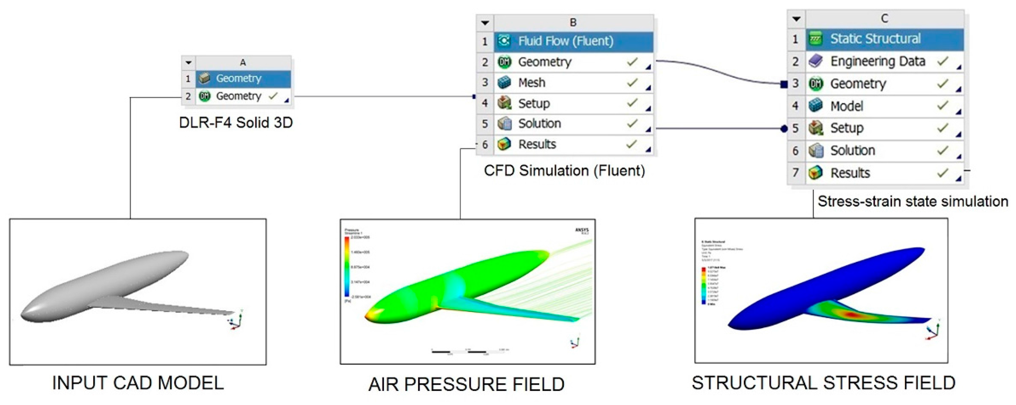
2.1. Methodology and Tools for CFD and Structural Stress Simulation

The task of numerical simulation of air flow over the wing cantilever, and its stress-strain state under aerodynamic loads, was solved in ANSYS Workbench environment, allowing a combined simulation of the model using several modules from different disciplines, including a full analysis of the interaction of gas dynamics with the wing structure, and aeroelasticity phenomena. The project scheme, presented in Figure 1 shows the steps of a one-way data interchange between different modules: first, the initial solid 3D model is transmitted from the geometry CAD module to the aerodynamic calculations module (Fluent), where the mesh settings of airspace domain around the model are configured, and CFD calculations are performed. The solution, including air pressure field on the wing surface, is then transferred to the static structural strength calculation module, where the grid of the internal structure of the model is built, and its static stress-strain calculation is carried out. If any changes are applied to the original input geometry (a modified winglet twist angle for instance), subsequent modules automatically update the grid and recalculate.

Governing Equations

For steady flow external aerodynamics, ANSYS Fluent solves conservation equations for mass—the continuity equation: $\nabla .(\rho \overrightarrow{v})=0$, and for momentum [28]:

$$\nabla .(\rho \overrightarrow{v}\overrightarrow{v})=-\nabla p+\nabla .(\overline{\overline{\tau }})$$

The continuity equation in the general form given above is valid for both incompressible (M ≤ 0.3), and compressible flows. Flow over the three-dimensional DLR-F4 wing-body configuration at a high subsonic velocity M = 0.6~0.85 involves compressibility, therefore, an additional energy conservation equation is solved:

$$\nabla .(\overrightarrow{v}(\rho E+p))=\nabla .\left[k_{eff}\nabla T-({\displaystyle \sum _j{h}_j{\overrightarrow{J}}_j})+({\overline{\overline{\tau }}}_{eff}.\overrightarrow{v})\right]$$

The complete system of governing equations and their underlying physical principles are given by Anderson [29]. The compressible viscous flow density was treated by the ideal-gas law: $\rho =P_{abs}/(R/M_{w}T)$, while the viscosity was calculated through Sutherland approximation:

$$\frac{\mu }{{\mu }_0}=\frac{T_{ref}+S}{T+S}{\left(\frac{T}{T_{ref}}\right)}^n$$

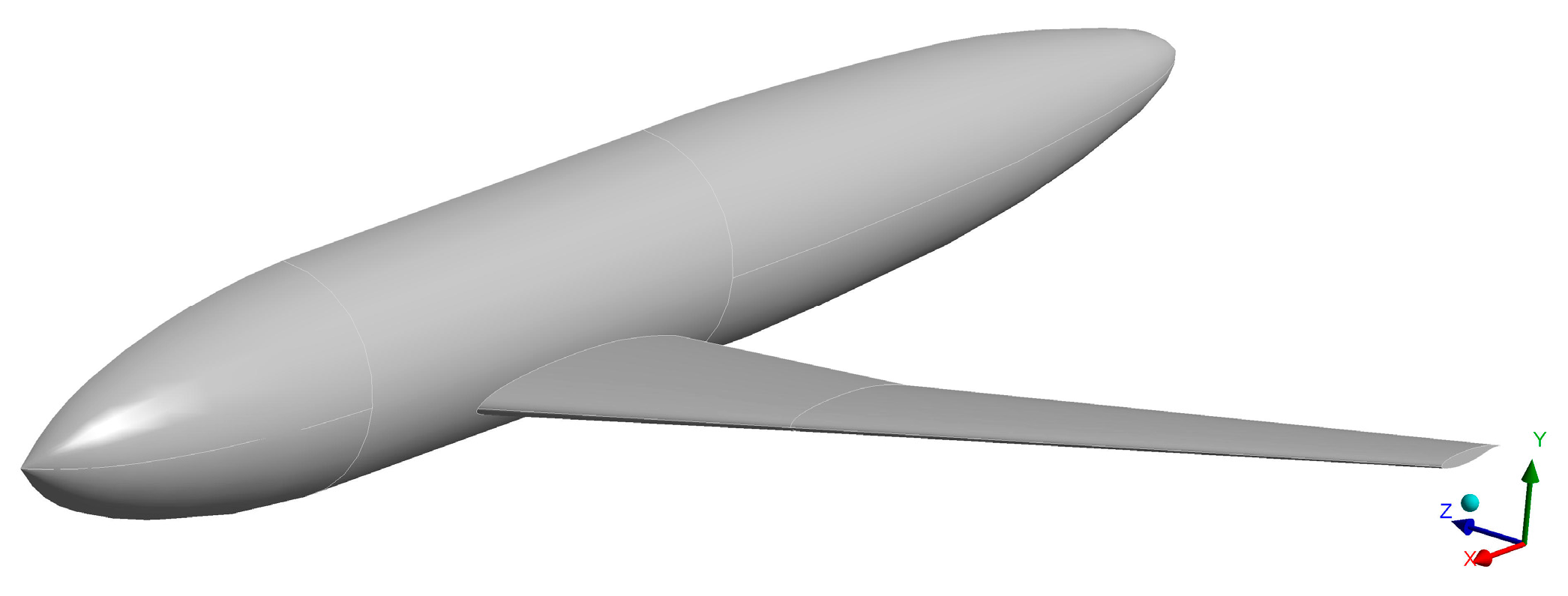
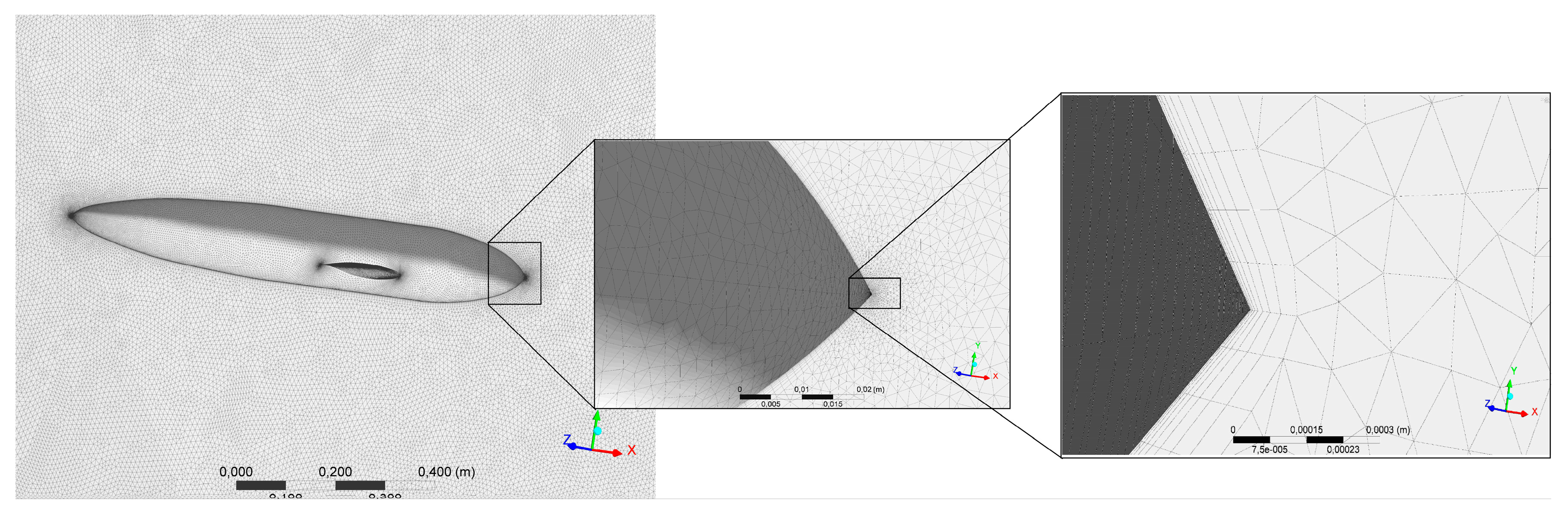
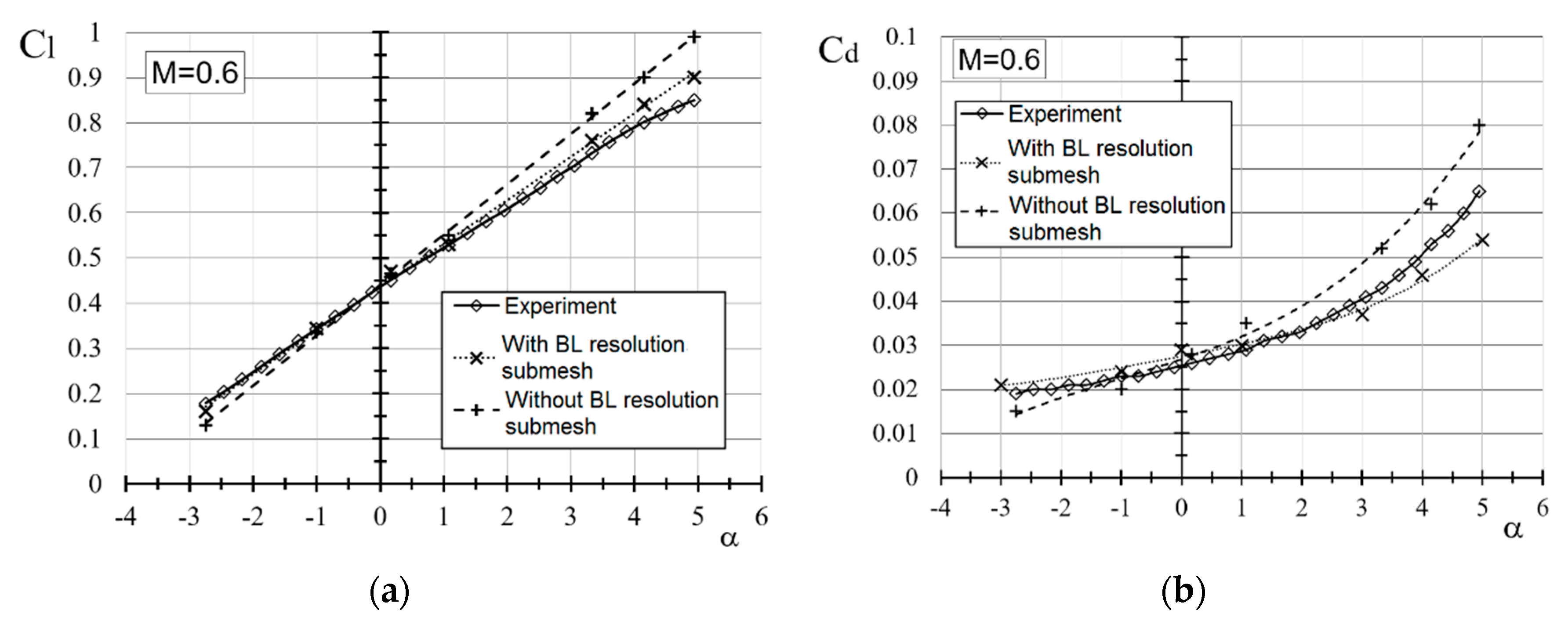
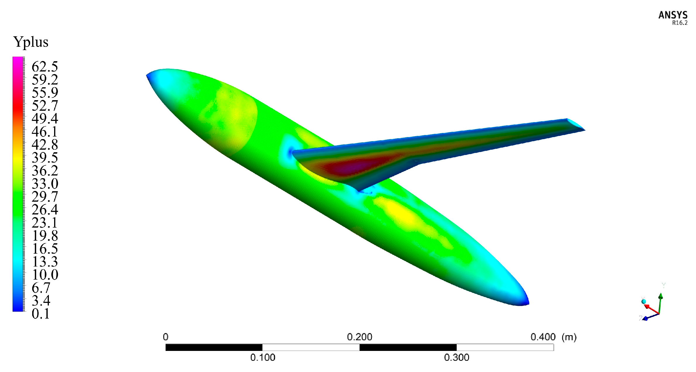
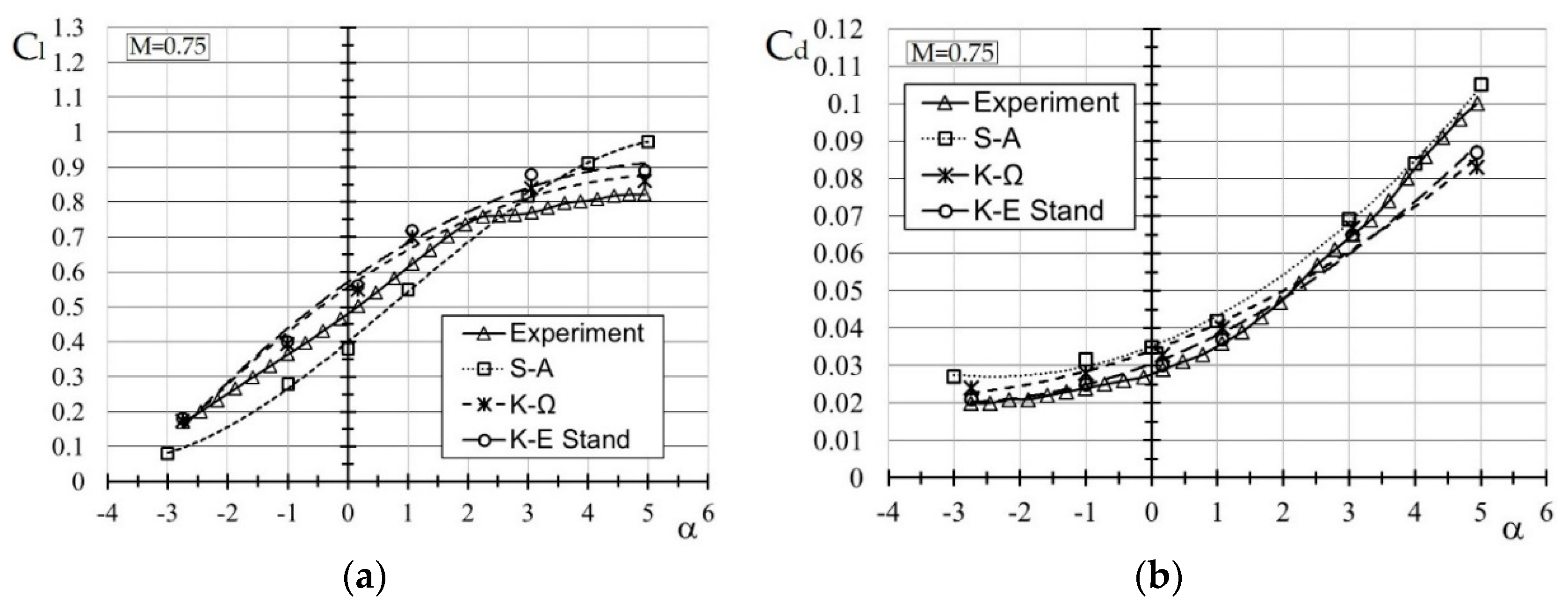
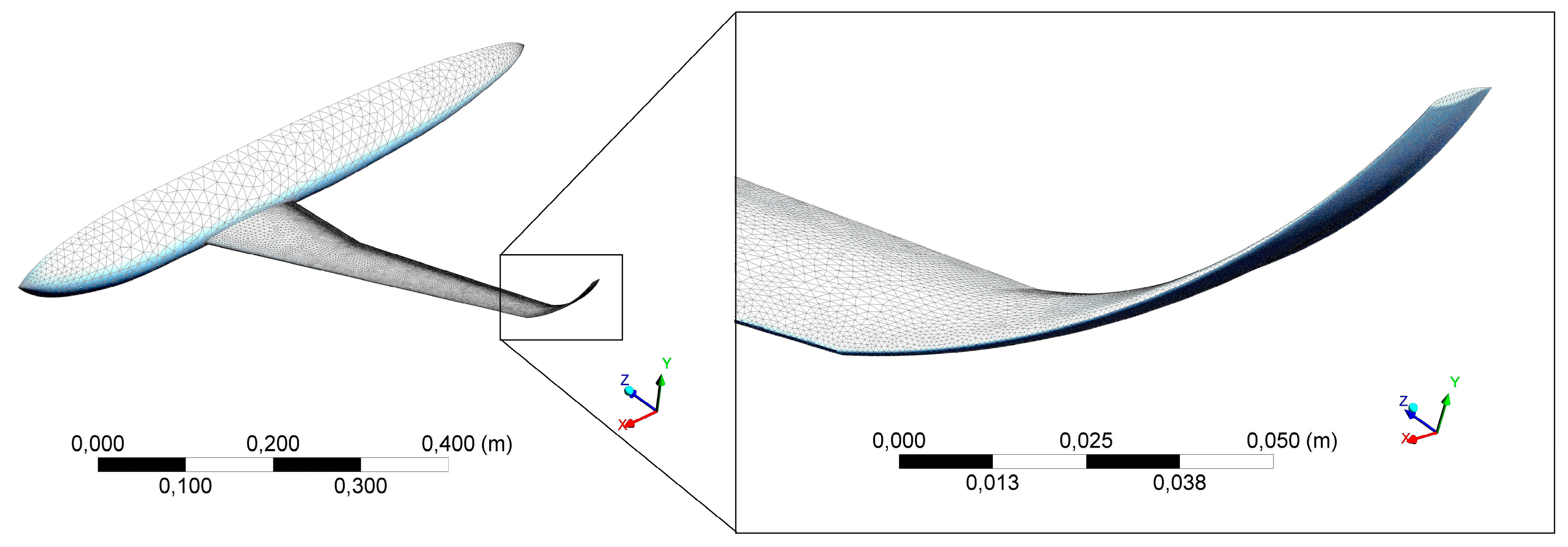
2.2. General Description of DLR-F4 Simulated Model and Mesh Convergence Study

DLR-F4 prototype, consisting of a fuselage in the form of a solid of revolution and a large aspect ratio swept back wing of a tapered planform, featuring a supercritical airfoil DFVLR R-4, allows the aerodynamic simulation of a typical medium-range subsonic passenger aircraft configuration. Using the DLR-F4 CAD model shown in Figure 2 as initial input, the influence of different winglet configurations on overall lift, drag and aerodynamic loads on the wing were studied. The impact of different cant angles for a classical Whitcomb winglet was identified in Mach number range of M = 0.6~0.87, with Reynolds’ number being equal to $Re=3\times {10}^6$.

As a reference area for calculating the aerodynamic coefficients of lift and drag, the wing plan area was taken including its ventral (non-wetted) part S = 0.148 m². The dimensions of the simulated domain and the mesh resolution were chosen to match the materials presented at AIAA CFD Drag Predictions (DP) seminars, for instance [30,31]. The simulated domain dimensions were five body lengths along the symmetry axis of the model, 2.6 body lengths along the vertical axis and 2.5 body lengths along the z-axis. The mesh size varied from seven to 20 million cells. Standard k-ϖ turbulence model provided acceptable accuracy with reasonable computational cost. The standard k-ϖ turbulence model is founded on the developed by Wilox [32] modifications for low-Reynolds-number effects, compressibility, and shear flow spreading, where the following transport equations allow obtaining the turbulence kinetic energy, k:

$$\frac{\partial }{\partial t}(\rho k)+\frac{\partial }{\partial x_i}(\rho k{u}_i)=\frac{\partial }{\partial x_j}({\mathsf{\Gamma }}_k\frac{\partial k}{\partial x_j})+G_k-Y_k$$

and the specific dissipation rate, ϖ:

$$\frac{\partial }{\partial t}(\rho \omega )+\frac{\partial }{\partial x_i}(\rho \omega u_i)=\frac{\partial }{\partial x_j}({\mathsf{\Gamma }}_{\omega }\frac{\partial \omega }{\partial x_j})+G_{\omega }-Y_{\omega }.$$

For CFD calculations on ANSYS FLUENT, an unstructured grid was used, consisting of tetrahedral cells condensing towards the surface of the wing-body, around which a structured sub-mesh was inflated allowing for a suitable boundary layer resolution. Parameters of the sub-mesh were set as 15 layers with a growth factor of 1.5, so that for each 10% body length, the resolution of the boundary layer could be ensured by at least 20 grid cells. Typical fragments of the domain mesh used in gas dynamics calculations are shown in Figure 3 below.

The influence of the inflated boundary-layer-resolution structured submesh on lift and drag computational results is illustrated by the comparison with wind-tunnel experimental results in Figure 4, where its effect on drag prediction accuracy becomes evident at high angles of attack up to 4°. An example of the wall Y-plus distribution is given at Figure 5 for the baseline model without winglets.

The results (which are available at open source website of AGARD (Advisory Group for Aerospace Research and Development)) of wind tunnel experiments conducted during 1994 at DLR (Germany), ONERA (France), DRA (UK) and National Aerospace Laboratory of the Netherlands [30,31], allowed a verification of the robustness of our research technique, and validate the selected boundary conditions, mesh resolution, and turbulence models for the Mach and Reynold’s numbers’ ranges corresponding to typical climb and cruising flight mode conditions, a comparison of ANSYS Fluent computational results using different turbulence models with selected AGARD experimental results from [33,34] is given at Figure 6 below for the lift and drag coefficients at flight angles of attack.

To calculate the increments of aerodynamic loads on the wing in ANSYS Static Structural finite element solver, an unstructured mesh for the inner structure of the model was also built from tetrahedral cells, where a high resolution mesh was set only for the wing structure, being the main object for stress-strain analysis in this paper, with proximity and curvature refinement. While for the fuselage body, a coarse grid was constructed and the boundary condition “fixed” was set, allowing zero-displacements in space under external loads. This simulates the weight of an aircraft fuselage, and allowed us to obtain aerodynamic wing loading values close to those loads encountered during a steady level flight. For static stress analysis, the total number of cells of the inner mesh of the wing and body combined is ~1 million. An example of a typical grid used in stress calculations is shown in Figure 7.

There are virtually no open source winglet prototypes available for a known transport airplane configuration with a known optimal geometry, or known empirical equations relating the winglet efficiency to its geometrical parameters. Thus, for an initial assessment of the influence on overall DLR-F4 aerodynamics of various geometric dimensions and setting angles of the winglet, and for their optimal choice in further work, a brief exploratory study of the design space of both a triangular wingtip fence and a classical winglet prototype was carried out, and a mathematical model was developed.

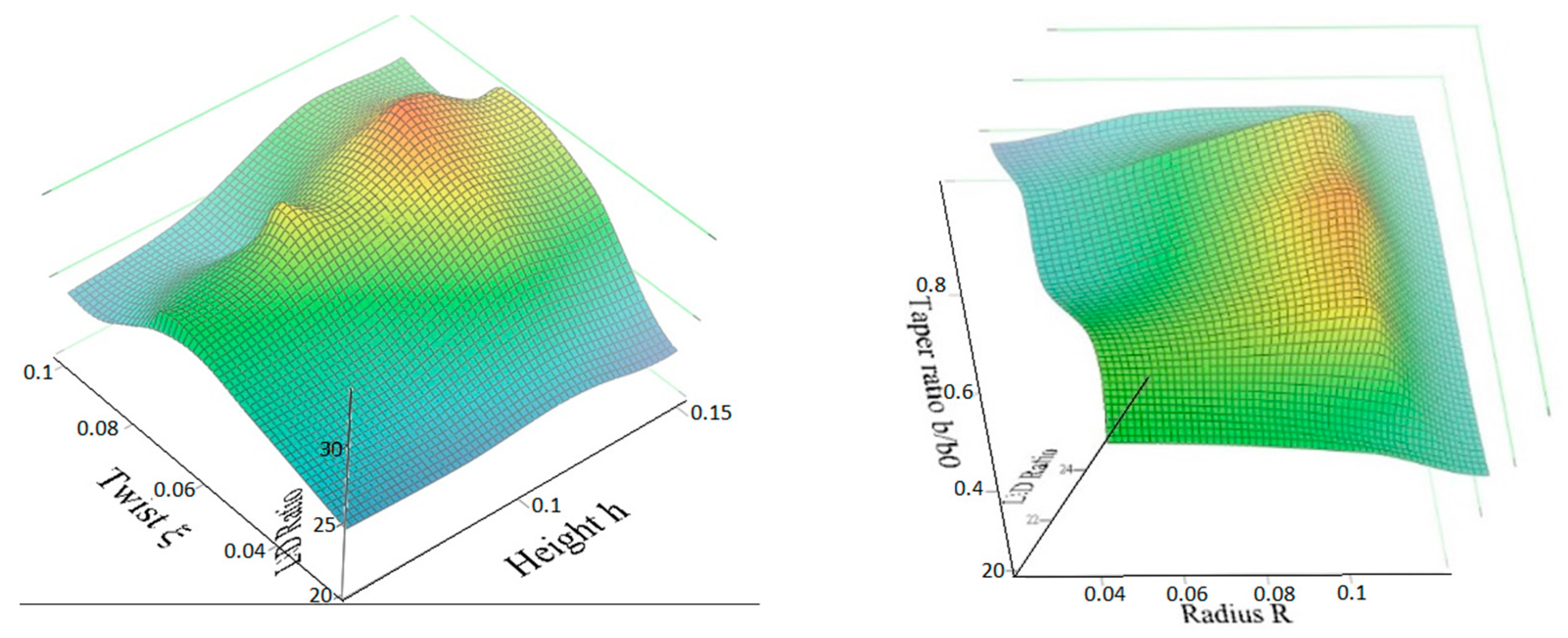
2.3. Design Space Exploration for Different Wingtip Device Geometries

In design optimization theory, the notion of design space of a system denotes the totality of all the values of geometrical dimensions and setting angles that are subject to free adjustment. A degree of freedom for a wingtip device geometry corresponds to a geometrical parameter; changing within certain limits affects the overall aerodynamic efficiency of the wing + wingtip device system. The growth in the lift-to-drag ratio L/D at cruising flight conditions as compared to the initial model without winglets was chosen as the main criterion for winglet geometry analysis and optimization.

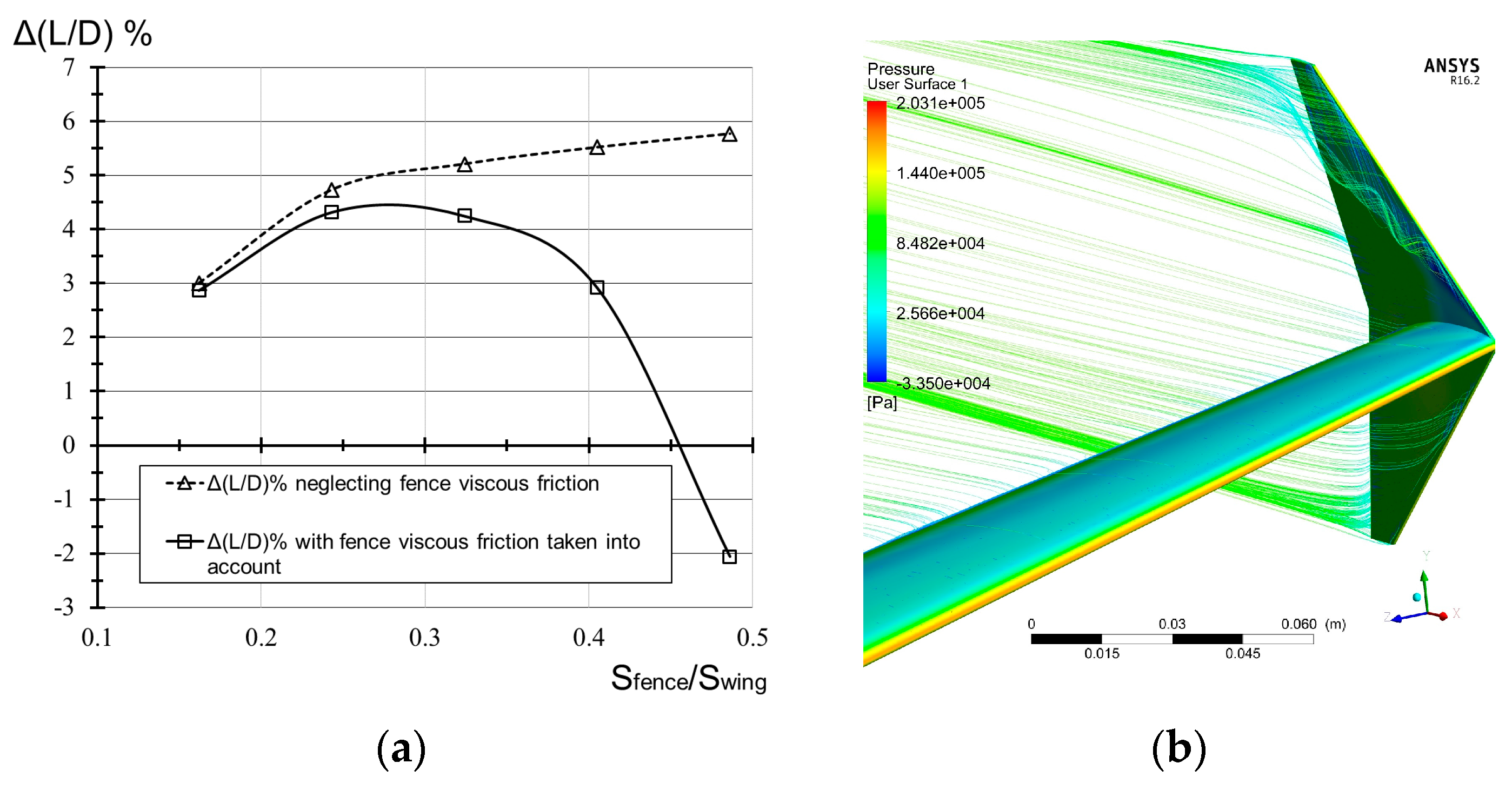
2.3.1. Wingtip Fence Design Space

For a two-dimensional delta planform wingtip fence (Figure 8b), based on theoretical considerations and wind tunnel experiments performed at [35,36], the key to L/D ratio growth of a wing equipped with a thin-airfoil tip fence is a large relative area of the wingtip fence S_fence/S_wing. While the remaining dimensions, the height and aspect ratio, have relatively little effect on its efficiency. Thus, we have a one-dimensional design space, where L/D ratio growth is directly proportional to the wingtip fence relative area S_fence/S_wing. However, S_fence upper values are limited by losses due to viscous friction of large fences (S_fence/S_wing ≥ 0.3), that can well exceed the gains in induced drag. Further increasing the fence area leads to a smaller growth, and eventually to a fall in the L/D ratio (Figure 8a, solid line). CFD calculations of the aerodynamic coefficients of DLR-F4 model equipped with few oval planform (for simplicity) endplates, aimed at finding near optimal values of a wingtip fence plan area, showed that the optimal endplate relative area lies in the range: [S_fence/S_wing]^optimal ~0.25 to 0.3. These results were taken into account for subsequent CFD and structural stress investigations of this near-optimal delta planform wingtip fence.

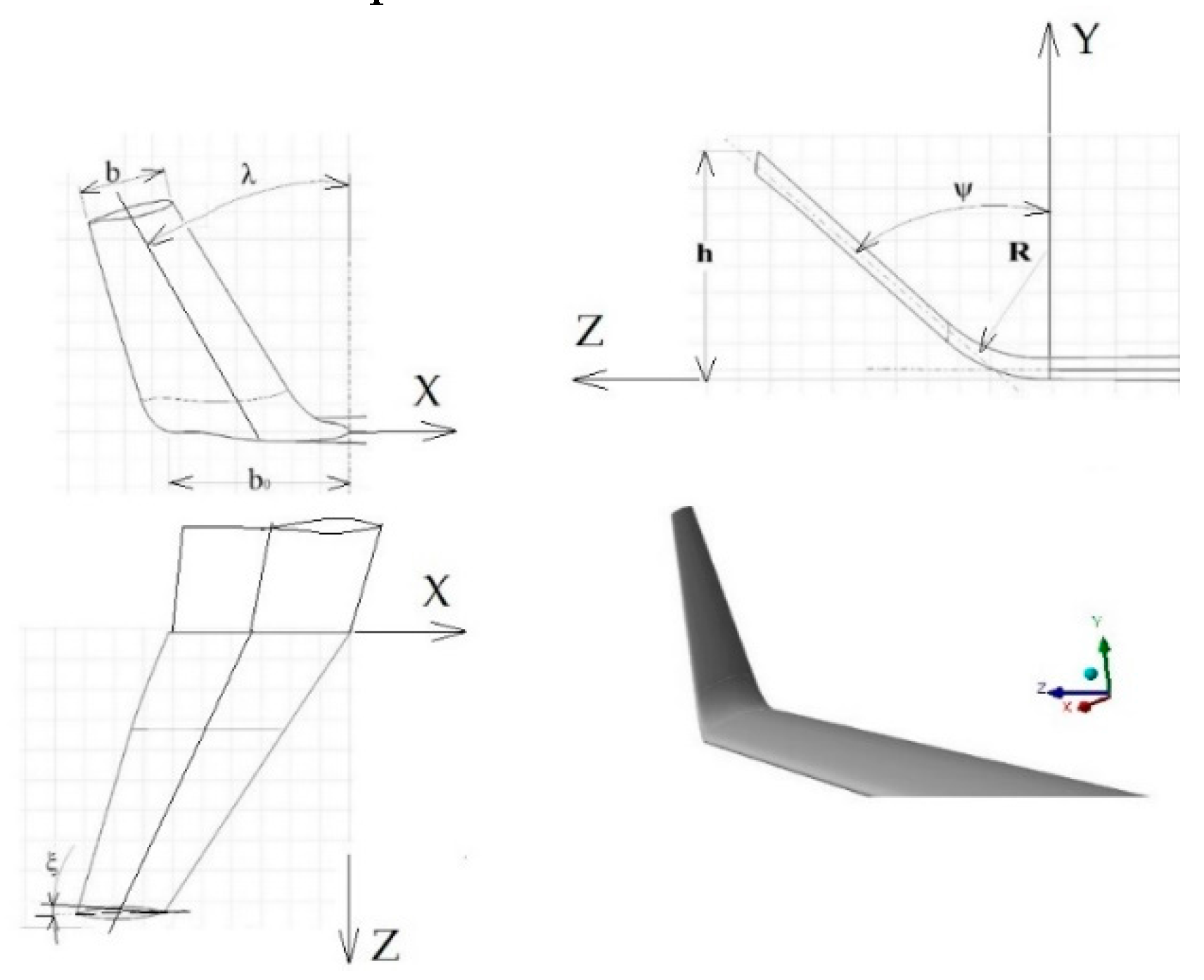
2.3.2. Winglet Design Space

A classical winglet is unlike the ‘flat’ wingtip fence shown above. Whitcomb winglet is a complex three-dimensional lifting surface with at least six geometrical parameters: sweep λ, cant ψ and twist ξ angles, the height h, fillet radius R and the taper ratio B = b/b₀ (Figure 9). In the coordinate system z-axis denotes the wing span direction perpendicular to the aircraft (XY) symmetry plane, x-axis: the direction of flight and y-axis normal to XZ plane: the normal force direction.

With over six degrees of freedom of the winglet design space, it is not viable to explore the whole design space by manual variations of each dimensional combinations. In order to best explore the vast multitude of possible combinations of input parameters, automated optimization simulations were carried out using ANSYS Design Exploration tool on relatively coarse grids for computational cost economy. In Figure 10 below, we show an example of surfaces estimating the effect on aerodynamic efficiency of winglet-equipped DLR-F4, of combined variations of both the winglet height (m) with twist (rad) and fillet radius (m) with taper ratio (dimensionless).

Despite relatively low accuracy coarse grids, response surfaces in Figure 10 allowed us to unveil the optimal envelope for values of the winglet geometrical parameters. This in turn allowed us to narrow the winglet six-dimensional design space to only one-dimension, where for further high-accuracy CFD investigations and loads or structural stress evaluation, it is sufficient to independently only vary parameters that mostly influence the L/D ratio and wing root bending moment, while keeping the values of other dimensions fixed. As for airfoiled winglets, it was shown that L/D ratio, as well as the wing root bending moment and as a result, span wise stress magnitude and distribution, are mostly sensitive to the winglet cant angle ψ (see Section 3.1.1 and Section 3.2). It is worth noting that using response surfaces, it is possible to optimize the winglet geometry for both maximum L/D ratio, and minimum wing root bending moment at the same time varying all six variables at once, but the computational cost would be unreasonably expensive, compromising the fidelity of results. Thus, a high fidelity cant angle ψ CFD and mathematical optimization was prioritized over other geometrical parameters to get a cost effective, ‘multi-fidelity’ approach.

2.3.3. Mathematical Modeling of the Winglet Local Flow Field

Given the winglet is an airfoiled finite-span lifting surface, finite wing theory can be applied to describe the three-dimensional flow field in its vicinity. In this paper, the winglet surface local flow field has been quantitatively analyzed through the term of the winglet local angle of attack ${\alpha }_{winglet}$, which is different in each section of the winglet (z) and generally assumed to be a function of both the winglet geometry, mainly the cant $\psi$ and twist ${\xi }_{winglet}$ angles, and the general angle of attack ${\alpha }_{wing}$ of DLR-F4 model, as well as three-dimensional flow field variables:

$${\alpha }_{winglet}={\xi }_{winglet}(z)+K_{\psi }{\alpha }_{wing}+{\alpha }_{flow\_field}$$

(1)

Here, the first and the second terms are geometric, while the third term arises from the three-dimensional flow field over the winglet span. In general:

• ${\xi }_{winglet}(z)$: the winglet twist, a function of z coordinate (changes spanwise): ${\xi }_{winglet}(0)=0$ means no twist at the winglet root. By convention, an outward twist at some z_n coordinate, which leads to an increased local ${\alpha }_{winglet}(z_n)\ge {\alpha }_{winglet}(0)$, is considered positive: ${\xi }_{winglet}(z_n)\ge 0$.
• $K_{\psi }$: Cant coefficient accounting for the winglet angle of attack ${\alpha }_{winglet}$ sensitivity to changing the general angle of attack of the model (or the wing) $\alpha ={\alpha }_{wing}$, which is linked to the cant ψ as follows: omitting both ${\xi }_{winglet}(z)$ and ${\alpha }_{flow\_field}$ (definition below), $K_{\psi }$ can be found from (1) and the assumption that increasing the angle of attack of a wing equipped with a vertical winglet ($\psi =0$, see Figure 9) does not increase the angle of attack of the winglet itself ${\alpha }_{winglet}^{vertical}=const$ (as a vertical winglet would be rotating over z axis in its own plane, experiencing a greater slip instead). From (1): $K_{\psi =0}=0$. While for a horizontal winglet ($\psi =\pi /2)$, the winglet angle of attack is directly equal to the wing angle of attack $\Delta {\alpha }_{winglet}^{horizontal}\approx \Delta {\alpha }_{wing}^{}$ (a horizontal winglet is just an extension of the wing itself), from (1) this means $K_{\psi =\pi }=1$. Solving the system of equations:

  $$\left\{\begin{array}{c}{K}_{\psi =0}=0,\mathrm{we}\mathrm{can}\mathrm{conclude}\mathrm{that}:K_{\psi }=\frac{\psi }{\pi /2}\hfill \\ K_{\psi =\pi /2}=1\hfill \end{array}\right\}.$$

  (2)

Only positively canted winglets were considered in this paper, where $\psi$ is ranged from $0\le \psi \le \frac{\pi }{2}$, which implies: $0\le K_{\psi }\le 1$. (2) can be verified for a half-canted winglet ($\psi =\pi /4$): $K_{\psi =\pi /4}=\frac{\pi /4}{\pi /2}=0.5$. This means that for any increase of the general angle of attack, half of that increase will contribute to geometrically increasing the winglet angle of attack: $\Delta {\alpha }_{winglet}^{\psi =\pi /4}=0.5\Delta {\alpha }_{wing}$.

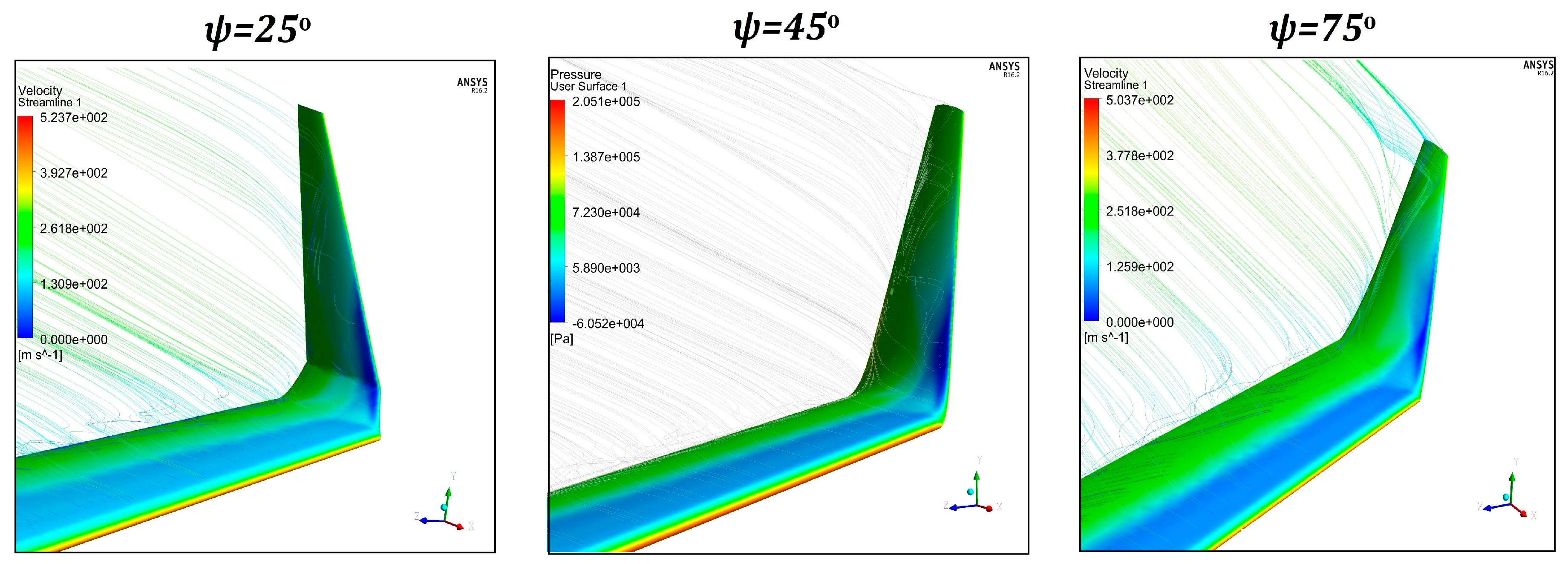
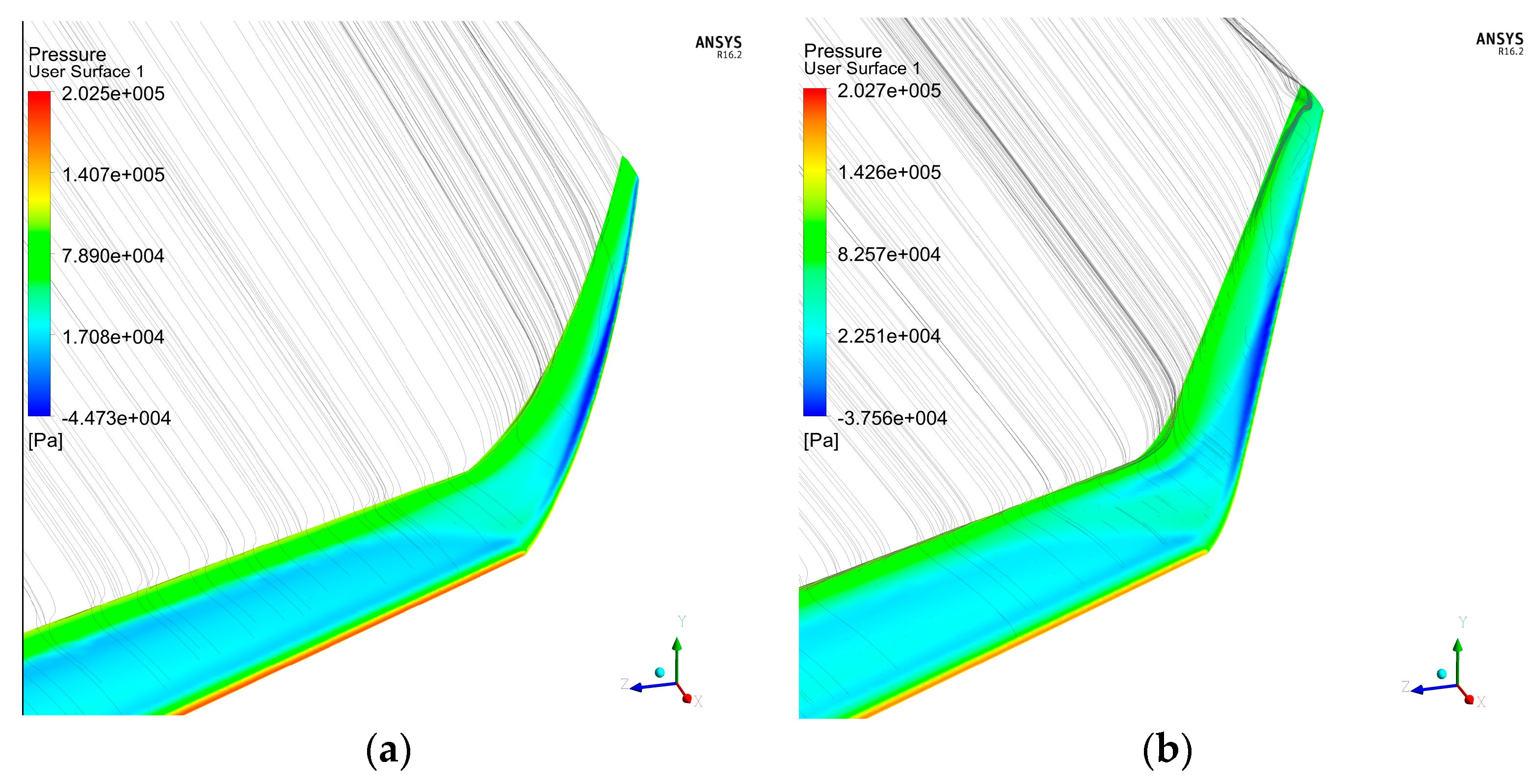
• ${\alpha }_{flow\_field}$ accounts for three-dimensional flow field near the winglet, involving a strong interference with the main wingtip vortex, which tends to increase local ${\alpha }_{winglet}^{root}$ at the winglet root sections (this can be clearly seen in Figure 11, where a substantially lower pressure on top winglet surface near the leading edge close to the wing junction). On the other hand, the winglet’s own ‘downwash’ and its smaller own tip vortex, lead to a slight decrease in local ${\alpha }_{winglet}^{tip}$ at the winglet tip sections. The interaction between the tip vortex and angle of attack has been studied in [37,38], and a method for predicting local root and tip variations, using local induced velocities is given in [39]. For a fixed winglet geometry at a fixed ${\alpha }_{wing}$, ${\alpha }_{flow\_field}$ is a function of the location on the winglet span (z coordinate):

  $${\alpha }_{flow\_field}={\alpha }_{flow\_field}(z)$$

  (3)

Substituting (2) and (3) in (1), a non-twisted (${\xi }_{winglet}(z)=0$) winglet local angle of attack would be:

$${\alpha }_{winglet}=\left(\frac{\psi }{\pi /2}\right){\alpha }_{wing}+{\alpha }_{flow\_field}(z)$$

(4)

Finding the exact ${\alpha }_{flow\_field}(z)$ function is beyond the scope of this paper, but its general shape has been approximately estimated for the non-twisted winglet shown in Figure 11, featuring a cant of $\psi =\frac{\pi }{4}$, CFD-simulated at Mach number M = 0.8 and ${\alpha }_{wing}=2°$~0.0349 rad. Substituting the values of $\psi$ and ${\alpha }_{wing}$ in (4), the local ${\alpha }_{winglet}$ for this winglet depends on the location z, in the same fashion as ${\alpha }_{flow\_field}(z)$ does, with a spanwise constant geometrical half α ‘cant correction’ of 0.0174:

$${\alpha }_{winglet}^{\psi =\pi /4}(z)={\alpha }_{flow\_field}(z)+0.0174$$

(5)

From (5) we can assume that the ${\alpha }_{winglet}(z)$ and ${\alpha }_{flow\_field}(z)$ should have the same graph shape. Computationally, this shape can be qualitatively obtained using the winglet surface pressure field and velocity vectors as shown in Figure 11 below. An optical method for experimental wind tunnel measurement of the local angle of attack is described in [40].

The mathematical model and Equation (4) described in this item will be particularly useful in interpreting the results of CFD simulation of few non-twisted winglets with different cant angles, and subsequently in the task of optimizing the cant angle for sustaining L/D ratio growth of DLR-F4 + winglet model at high angles of attack.

3. Results

3.1. CFD Simulation Results of the Winglet-Equipped DLR-F4 Model

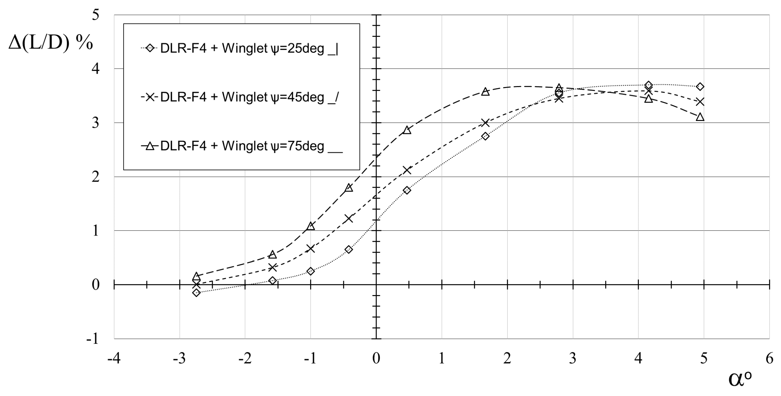
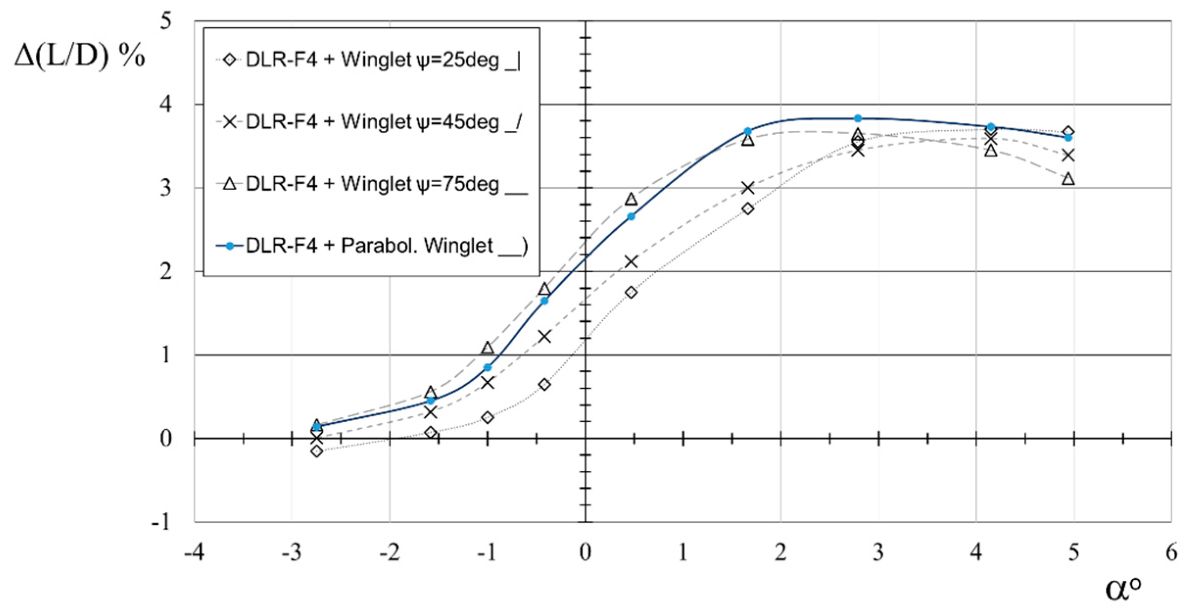
3.1.1. Impact of the Winglet Cant Angle on DLR-F4 Lift-to-Drag Ratio

As shown in Figure 12 below, dependence on the angle of attack of overall growth in L/D ratio (%) of the model equipped with winglets of different cant angles, as compared with initial DLR-F4 without winglets, we can confirm the positive effect of this wingtip device on DLR-F4 L/D ratio at flight angles of attack (up to ~4% gain). Winglets with larger cant angles generally perform better, due to higher lifting characteristics excepted at high and close to critical angles of attack where nearly vertical winglets (ψ = 25°) slightly prevail, due to a better induced drag reduction (acting as a vertical fence better isolating upper and lower wing tips with largely different pressure values helps weaken wingtip vortex and hence induced drag).

From Figure 12, the influence of the winglet cant on DLR-F4 L/D ratio changes depending on the angle of attack of the model, ${\alpha }_{wing}=\alpha$. Highly canted winglets are more sensitive to increasing the angle of attack of the wing than nearly vertical winglets. This sensitivity is illustrated in Figure 13 below, where winglets with different cant angles are exposed to a high-subsonic air flow regime M = 0.8 at a high angle of attack. Streamlines reveal a flow separation, an intense tip vortex and a loss of efficiency for the winglet with ψ = 75° and, to a lesser extent the one with ψ = 45°. While the flow field behind the least canted winglet with only ψ = 25°, remains relatively smooth despite high angle of attack of the model.

3.1.2. Winglet Cant Optimization for a Sustainable Efficiency along α Range Using a Curved Span

From Figure 12 and Figure 13, a major problem of winglet design is the proper choice of a balanced cant angle that would prevent the flow separation and loss of efficiency in the winglet tip area at high α during take-off and climb, while providing acceptable lift at moderate α during cruise. Geometric twist is a well-known solution in correcting local α of lifting surfaces. A negative twist of the highly canted winglet’s tip sections, for instance, might be applied to geometrically reduce the tip local angle of attack and obtain a smoother pressure distribution, thus delaying flow separation at high α. However, exploratory studies performed at Figure 10 on relatively coarse grids revealed that twist correction is advantageous only at substantially high angles of attack. At smaller cruise angles of attack, a negatively twisted tip local angle of attack becomes too small, or even negative, leading to a substantial loss in L/D ratio. Thus, a twist-morphing concept might be considered, dynamically applying twist only at high α. Another, more efficient morphing is dynamic cant correction: shifting to smaller cant angles at higher angles of attack, thus dynamically reducing the cant coefficient $K_{\psi }$ (see Section 2.3.2, Equations (1) and (2)), making the winglet local angle of attack less sensitive to increasing the general angle of attack, and using the winglet as a vertical fence at high α. This can be achieved through a cant-morphing winglet. Several studies regarding morphing concepts were performed, see [11,12,13,26] for instance. In this paper, a much simpler and structurally lighter alternative is suggested that does not involve morphing, and therefore, no complex articulation mechanisms are needed: A curved winglet, where local cant angle is different at each section (highly canted root versus nearly vertical tip, with gradual transition in between, see Figure 14 below).

The curved winglet concept can be mathematically analyzed as follows: The curved winglet centerline front (YZ) projection should be parametrized using a second order function Y(z), where the graph is tangent to the wing at the wing-winglet joint. For instance, for a parabolic winglet as shown on Figure 15, the parametrization function is Y(z) = z². For a curved winglet, the constant cant of a straight winglet ψ should be replaced by a cant function $\psi (z)$, which gives the local cant spanwise at each point (From Figure 15, this is π/2 minus the slope of the tangent line of the parametrization function graph). Therefore, the cant function $\psi (z)$ can be calculated by deriving the chosen parametrization function as follows:

$$\psi (z)=\frac{\pi }{2}-\arctan [Y’(z)]$$

(6)

For the parabolic winglet case, the cant function is: $\psi (z)=\frac{\pi }{2}-\arctan [Y’(z)]=\frac{\pi }{2}-\arctan [\frac{1}{2}z]$, which can be verified at the winglet root: $\psi (0)=\frac{\pi }{2}-\arctan (0)=\frac{\pi }{2}={\psi }_{\max }$, which means that the local cant at the winglet root is the maximum possible. This complies with wing-winglet tangential connection requirement.

CFD simulation of the parabolic winglet confirmed its reduced sensitivity to high angles of attack, where the gain in L/D ratio remains the highest up until α = 5°. The solid graph at Figure 16 below, corresponding to the parabolic winglet shows that a curved winglet provides a compromise, performing nearly as good as highly canted winglets at small α, with a sustainable L/D growth at higher angles of attack.

Flow field visualization in Figure 17 clearly reveals the positive effect of the winglet curved span shape on the three-dimensional flow field, which now involves a much weaker tip vortex and a delayed flow separation. Pressure field on the top surface of the parabolic winglet, near the leading edge, reveals how the tip sections, being nearly vertical allow a better local angle of attack distribution spanwise, thus resulting in a smoother pressure distribution and a sustainable efficiency of the winglet tip sections.

3.1.3. Optimal Cant Function

For an arbitrarily shaped curved-span winglet, by replacing the constant cant ψ with a cant function $\psi (z)$, (4) becomes:

$${\alpha }_{winglet}=\left(\frac{\psi (z)}{\pi /2}\right){\alpha }_{wing}+{\alpha }_{flow\_field}(z)$$

(7)

Substituting (6) in (7), we obtain the winglet local angle of attack dependency on z for a non-twisted, arbitrarily shaped curved winglet, parametrized through an arbitrary second order function Y(z):

$${\alpha }_{winglet}=\left(\frac{\frac{\pi }{2}-\arctan [Y’(z)]}{\pi /2}\right){\alpha }_{wing}+{\alpha }_{flow\_field}(z)$$

which, given $\arctan [Y’(z)]$ in rad, reduces to:

$${\alpha }_{winglet}\approx \left[1-0.636\cdot \arctan [Y’(z)]\right]{\alpha }_{wing}+{\alpha }_{flow\_field}(z)$$

(8)

As was mentioned earlier, the winglet shape should be optimized for getting the highest possible, at all flight angles of attack, L/D ratio of DLR-F4 + winglet model. From (8), seeking the optimal shape of a curved winglet is seeking the optimal parametrization function Y(z)^optim, the derivative of which Y’(z)^optim, being substituted in (8) results in an optimal spanwise distribution of local ${\alpha }_{winglet}(z)$. In the light of CFD results shown at Figure 12 and Figure 13, Figure 16 and Figure 17 and the definition of the suggested spanwise-curved winglet solution (Section 3.1.2), this optimal ${\alpha }_{winglet}$ spanwise distribution can be achieved by ensuring, at the same time, the following three conflicting local winglet flow field conditions:

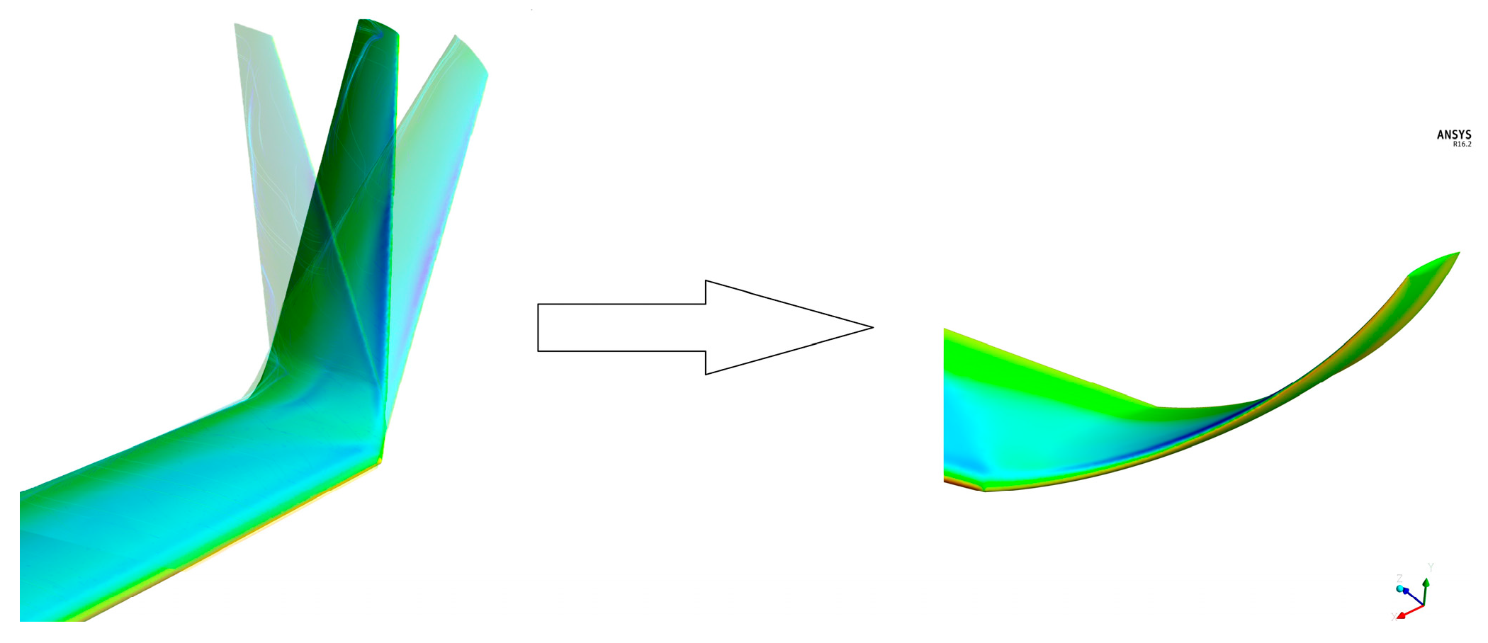
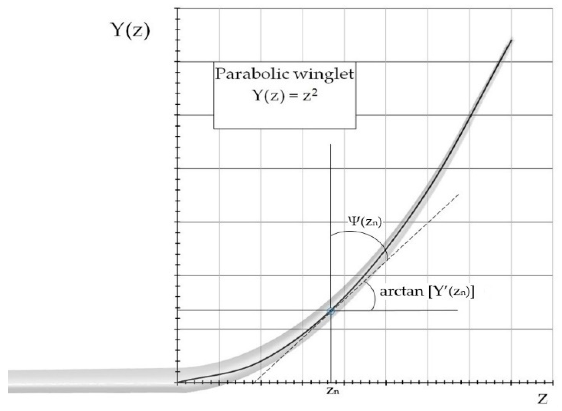
• Ensuring the highest possible, yet under critical, local angle of attack of the winglet: for a curved winglet design, this is interpreted as the highest cant possible at root, in order to best harness the main wingtip vortex energy (see Figure 11) and use it to increase local ${\alpha }_{winglet}^{root}$. Also, in order to get the highest possible local increase, should the wing angle of attack increases $\Delta {\alpha }_{winglet}^{root}\approx \Delta {\alpha }_{wing}^{}$ (see Section 2.3.2, Equation (2)). This highest cant ${\psi }_{\max }^{root}=\pi /2$ is achieved through a tangent connection to the wing at z_root = 0: ${\psi }^{opt}(0)=\frac{\pi }{2}$. Substituting in (6):

  $$\begin{gathered} {\psi }^{opt}(0)=\frac{\pi }{2}-\arctan [Y{’}_{optim.}(0)]=\frac{\pi }{2}\Rightarrow \arctan [Y{’}_{optim.}(0)]=0\Rightarrow \\ Y{’}_{optim.}(0)=0 \end{gathered}$$

  (9)
• Ensuring the smallest possible pressure difference between upper and lower surfaces at the winglet tip, thus keeping the winglet tip vortex and its own downwash at the lowest possible intensity. This can be achieved by making the tip vertical (with zero cant), in order to prevent its angle of attack from increasing (and the pressure difference from rising), should the general angle of attack increases: $\Delta {\alpha }_{winglet}^{tip}\approx 0$ (see Section 2.3.2). Hence ${\psi }^{opt}(z_{tip})=0$, Substituting in (6):

  $$\begin{gathered} {\psi }^{opt}(z_{tip})=\frac{\pi }{2}-\arctan [Y{’}_{optim.}(z_{tip})]=0\Rightarrow \arctan [Y{’}_{optim.}(z_{tip})]=\frac{\pi }{2}\Rightarrow \\ Y{’}_{optim.}(z\to z_{tip})\to \infty \end{gathered}$$

  (10)

  (10) means an infinite slope (vertical) tangent line to Y(z)^optim. graph at the at the winglet tip.
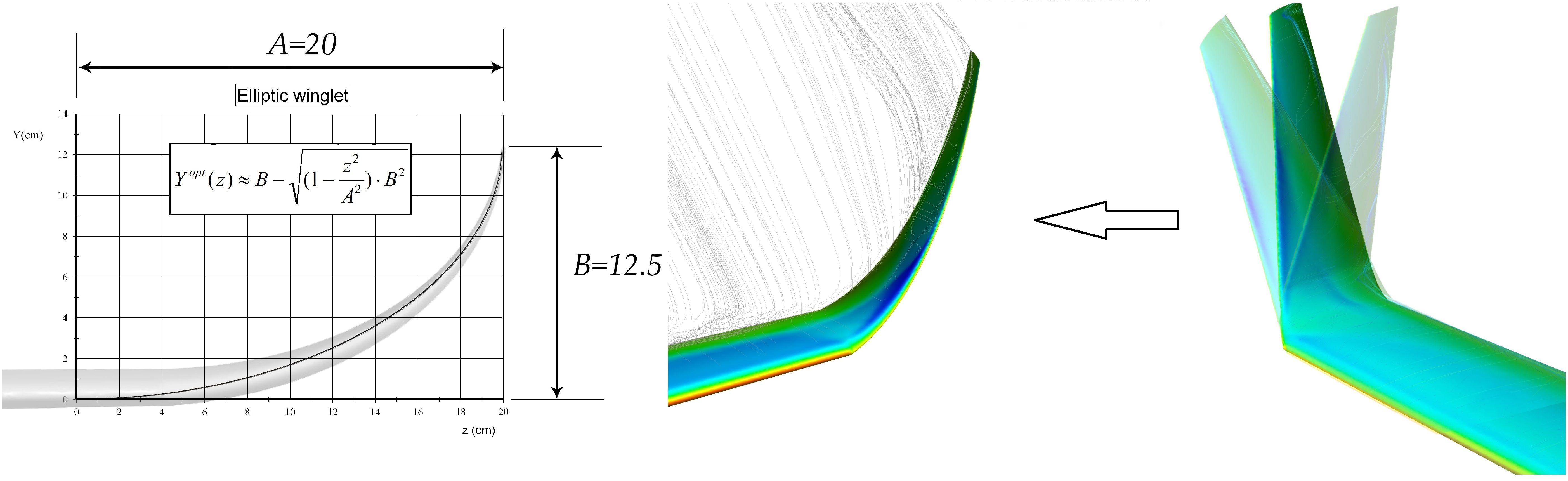
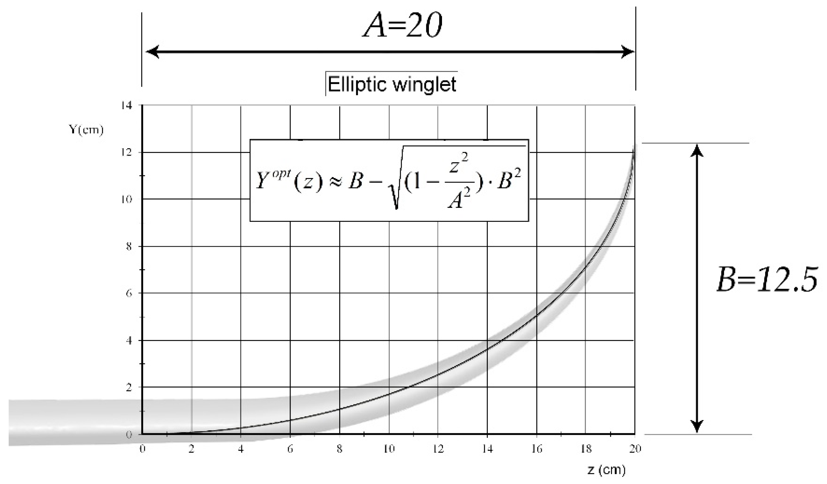
• Ensuring the most advantageous transition from ${\alpha }_{winglet}^{root}$ to ${\alpha }_{winglet}^{tip}$. From (8), this requires a well-known flow field dependency ${\alpha }_{flow\_field}(z)$; defining it is beyond the scope of this paper, see [37,39]. We can only notice that ${\alpha }_{flow\_field}(z)$ itself depends on the winglet geometry, meaning that the optimization process is iterative, starting from an arbitrary second order parametrization function, defining ${\alpha }_{flow\_field}(z)$ for it (either mathematically or experimentally), identifying an improvement direction, and then gradually adapting the parametrization function up until the point where L/D ratio does not grow anymore. It is well-known, however, that optimal spanwise circulation distribution of a lifting surface with the minimum induced drag is elliptical. Therefore, we may assume that a similar elliptic cant parametrization which easily complies with (9) and (10), would result in the highest L/D ratio of the winglet.

Given the boundary conditions from (9) and (10), as well as a mathematically optimal elliptic transition, an optimal curved winglet may be parametrized by a quarter ellipse function (Figure 18):

$$Y^{opt}(z)\approx B-\sqrt{(1-\frac{z^2}{A^2})\cdot B^2}$$

(11)

where: A and B correspond to the ellipse semi-major and semi-minor axes respectively.

For a known maximum wing span, which is usually the case for an operational aircraft, it is easy to define the semi-major axis A. For illustration, let’s assume that an operational DLR-F4 aircraft maximum allowable wing semi-span is $L_{\max }^{DLR-F4}=78.56\mathrm{cm}$. Initial DLR-F4 wing semi-span without winglet is $L_{without}^{DLR-F4}\approx 58.56\mathrm{cm}$, then $A=L_{\max }^{DLR-F4}-L_{without}^{DLR-F4}=20\mathrm{cm}$. The semi-minor axis B can be obtained from a fixed winglet height h = B. From response surfaces in Figure 10 let’s choose: h = B = 0.125 m = 12.5 cm.

Substituting A and B in (11):

$$Y_{optim.}^{DLR-F4}(z)=12.5-\sqrt{(1-\frac{z^2}{{20}^2})\cdot {12.5}^2}=12.5-\sqrt{156.25-0.39\cdot z^2}$$

The graph of this particular-case elliptic winglet is given at Figure 18 below.

It is worth noting that the concept presented herein of a spanwise-curved winglet is not completely new, and can be viewed as an extrapolation of the (already known to be efficient, see [9,22] for details) blended winglet concept, featuring an increased fillet radius and tangent wing joint. Airbus’s latest wide body airliner A350 features a similar curved winglet, while the Boeing 787 wing has its tip section elastically deformed upward in flight, resulting in a gradual transition to a lower local cant angle of its raked wingtips the closer we move to the tips [41].

The novelty of this research lies in the methodology used for quantitative analysis of the effect of various geometric parameters of the winglet, the cant angle in particular, through the analysis of their effect on the local angle of attack, which both geometrically and physically drastically varies from one section of the winglet to the other. This is important for winglet and non-planar wings design, because in comparison with the 3D flow field around a high aspect ratio wing such as DLR-F4 wing (which, far from the tips, can be replaced by a simpler 2D flow with constant-spanwise local α), the flow field around the winglet is deeply three-dimensional, dominated by a high intensity tip vortex from the wing, and the winglet’s own downwash.

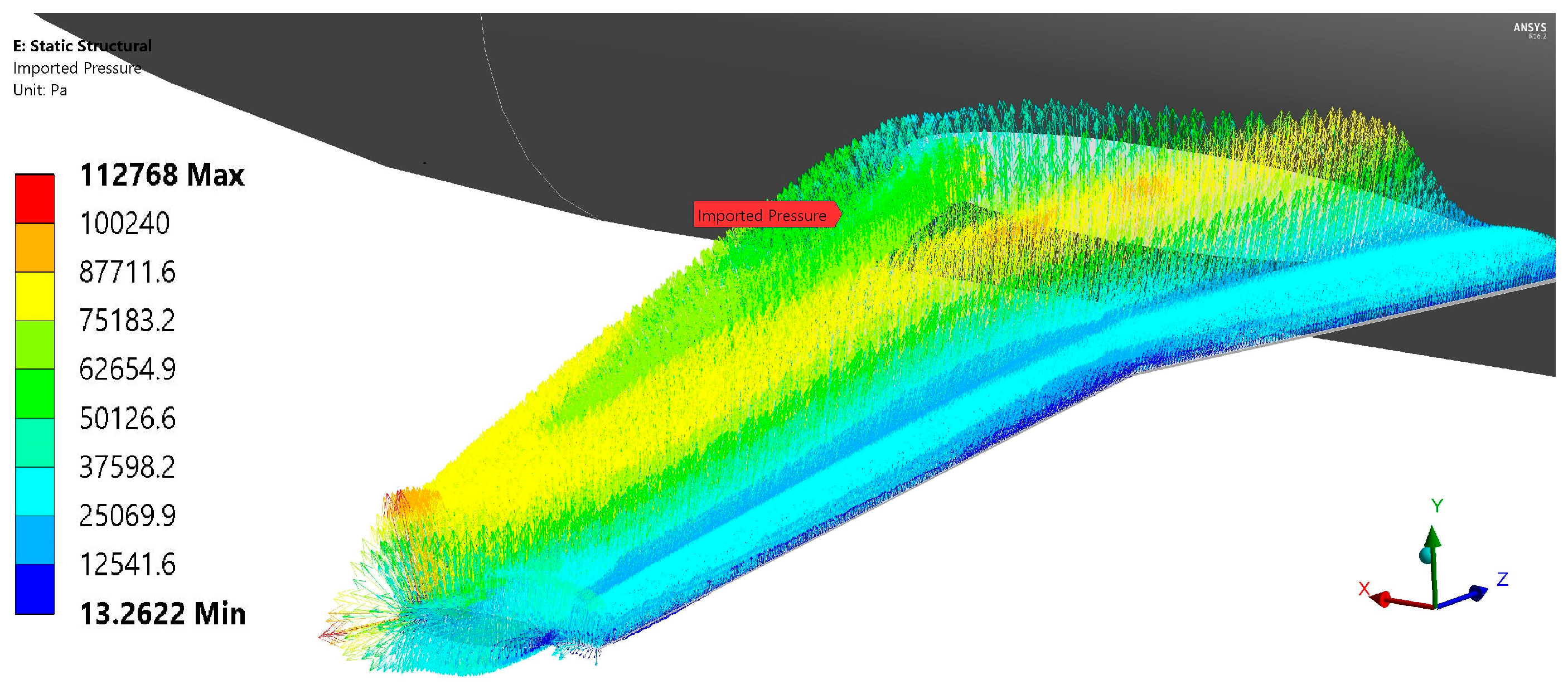
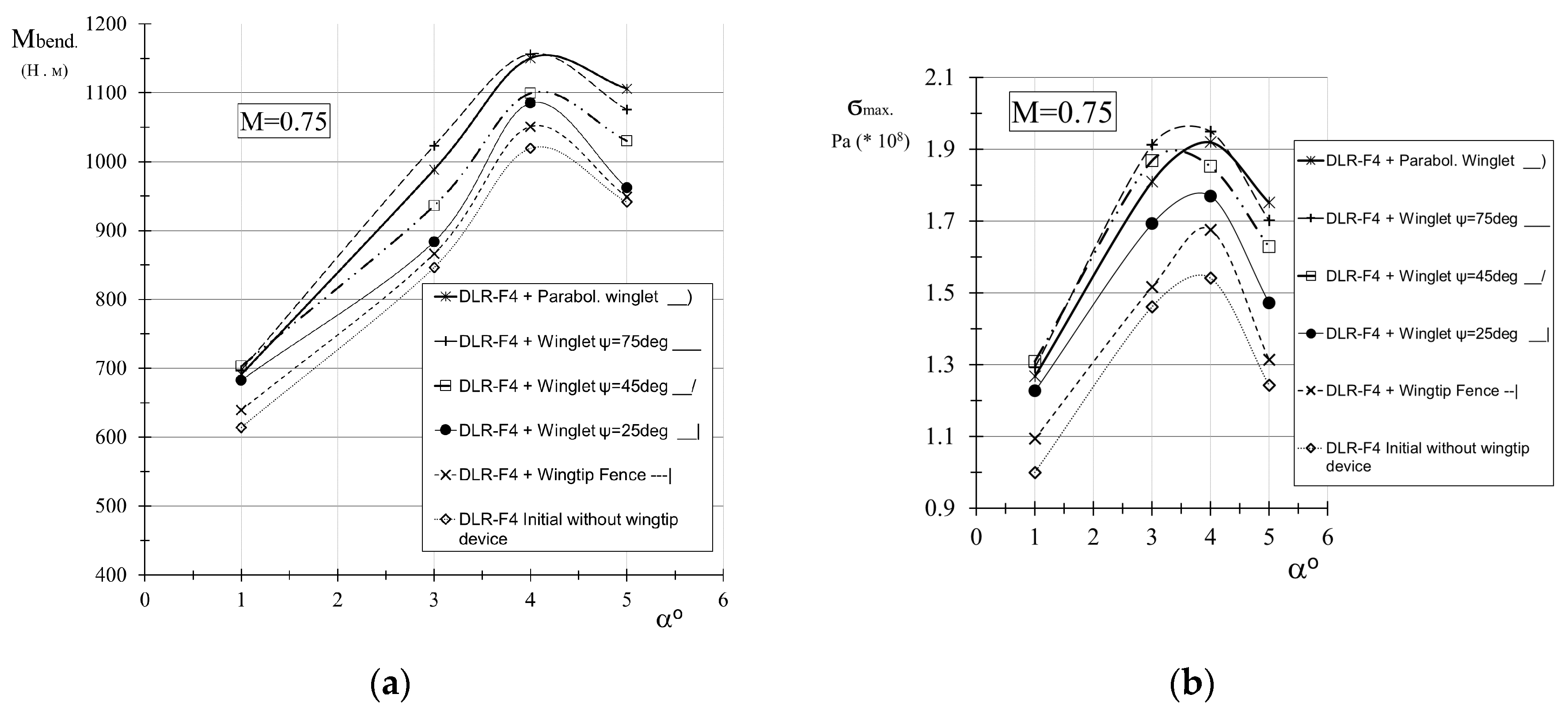
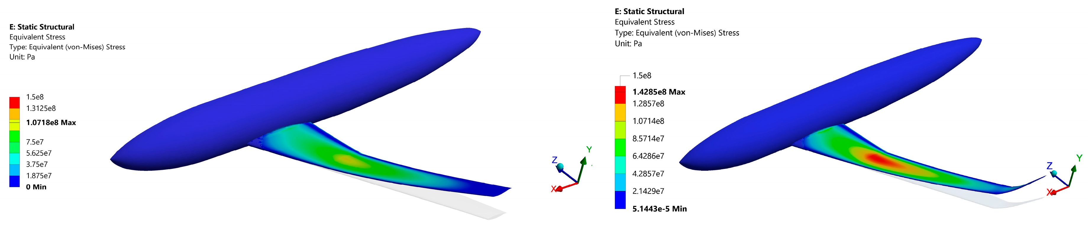
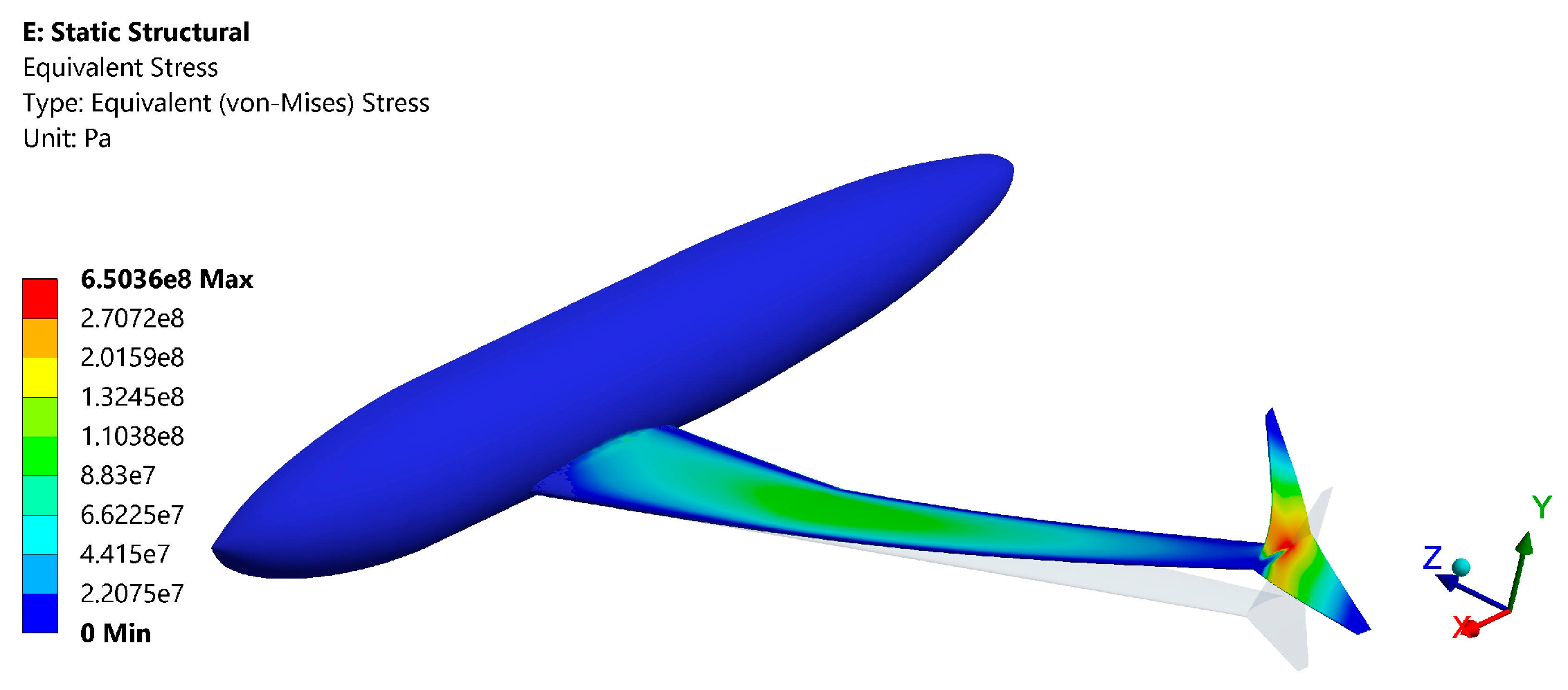
3.2. Stress-Strain State Simulation Results of Winglet-Equipped DLR-F4

Besides L/D ratio, another important result of CFD calculation is the air pressure distribution on the wing surface, which serves as the initial external loads input information for stress calculations on the wing cantilever. Physical experiments made by R. Whitcomb back in the 1970s [1,2], included an estimation of the growth of wing loading by integrating air pressure obtained from a large number of sensors over the wing and winglet upper and lower surfaces. In the course of computational experiments in this paper, a similar approach to sensors is used, where air pressure is read by the software for each of the individual surface mesh cells (Figure 19), and then integrated to calculate the aerodynamic loads.

In Figure 20, a comparison of the wing root bending moment (WRBM) values and maximum equivalent Von Mises stress for winglets of cant angles: ψ =25°, 45° and 75° is shown for a parabolic winglet, a delta planform wingtip fence and the initial DLR-F4 wing without wingtip device. Simulation was performed at positive angles of attack and Mach number of M = 0.75. From Figure 20a, we can conclude that the increase of wing root bending moment for winglets is directly proportional to the value of their cant angle. This can be explained by a greater additional lifting force, the highly canted the winglet is. Thus, the smallest increase in wing loading corresponds to the ‘non-lifting’ wingtip fence. At moderate angles of attack α~1°, all winglets cause virtually the same WRBM increment, but increasing the angle of attack, the bending moment increases at a slower pace the less canted the winglet is. This is a direct implication of the cant coefficient $K_{\psi }$ described in Section 2.3.2, Equations (1) and (2), which is greater for highly canted winglets, leading to a faster-pace growth in their angle of attack and subsequently greater lifting force acting on them, which in turn leads to a faster pace growth of WRBM. In this regard, the parabolic winglet, although causing relatively high WRBM values, offers a compromise solution up until α~3°. At α~4° and higher, WRBM growth becomes higher than for conventional straight winglets. This can be explained by the sustainable lift generated by its tip sections (compare top surface pressures at both the winglets’ tips at Figure 17).

WRBM is a central factor of wingtip device weight penalty, but the combined effect of all winglet-induced aerodynamic loadings increases in bending, torque moment and the shear force, can be more fully studied by evaluating the changes of both the value and distribution of structural stress along the wing span. For this purpose, structural steel was set as the material of a one-piece wing cantilever structure. As the study presented here is mainly for a comparison purpose, structural material choice and internal structural layout is not important so far. On Figure 21 below, an example is shown of 34% growth in maximum Von Mises stress due to the installation of a highly canted winglet with ψ = 75°, at M = 0.8 and α = 1°. According to experience of wing structural weight estimation for transport aircraft, a minimum resulted in wing box structural weight growth of 10% for an Al-alloy box structure, and at least 15% for a spared structure [42].

From Figure 20, we can assume that the optimal for structural weight penalty wingtip device is the wingtip fence. Thus, it can be retrofitted into most operational aircraft almost without the need for a wing structure rework. It should be noted, however, that ensuring the aerodynamically optimal fence relative area S_fence~0.27S_wing (based on the dependence shown earlier in Figure 8a), results in considerable local stress and deformations of the wingtip fence itself (Figure 22). This is due to the large plan area combined with an extremely small thickness (structural depth). Counter measures to locally strengthen the wingtip fence and its junction area with appropriate material choice are required, and they may lead to significant weight penalties.

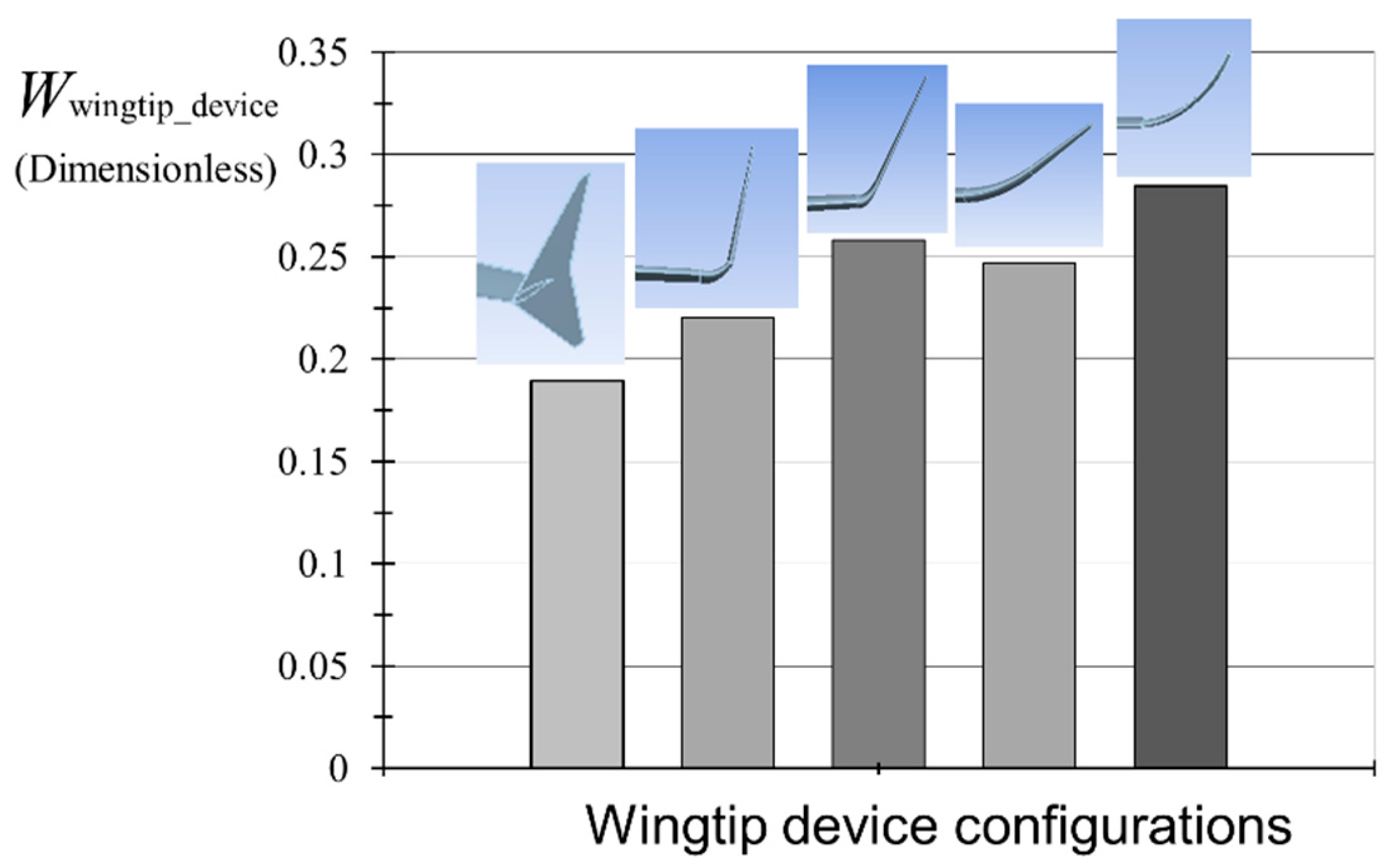
3.3. Developing a Multidisciplinary Criterion for Wingtip Device Aerodyamic Efficiency Assessment Regarding Structural Weight Penalty

Taking into account the conflicting nature of the influence of different wingtip devices on aircraft fuel efficiency, where we have a perceptible improvement in Lift-to-Drag ratio (up to 4–5%) at flight angles of attack and cruising Mach numbers on one hand, and a considerable increase in wing loading, involving a structural weight penalty on the other hand (Figure 20, Figure 21 and Figure 22). Also, given the vast design space and the multitude of choices available for a device geometry, decisions about wingtip device configuration made during the early stages of wing design should be guided by some practical design philosophy allowing to reach an acceptable level of wingtip device aerodynamic efficiency, keeping the weight penalty in mind. In this paper, a quantitative evaluation criterion is suggested, that measures the aerodynamic benefits of wingtip devices at cruising flight mode, responsible for most of the timespan of aircraft operation and where, as a result, even small improvements in aerodynamic efficiency yield significant long term savings for airlines. As a test condition for wingtip device weight penalty though, it is proposed to measure loads for mostly loaded flight modes, including off-design conditions. Since the wing structural strength is usually designed to withstand maximum, despite only occasionally occurring (or may never occur) aerodynamic loads, besides typical cruising loads.

Thus, for quantitative comparison of the aerodynamic benefits of different wingtip devices, regarding their structural cost, it is proposed to calculate and compare a dimensionless ratio denoted $W_{Tip\_device}$ of the increase in L/D ratio during cruising flight $\Delta {(L/D)}_{Cruise.}$(%) to the maximum possible (chosen from an off-design condition) growth of structural stress $\Delta {\delta }_{\max }$(%):

$$W_{Tip\_device}=\raisebox{1ex}{$\Delta {(L/D)}_{Cruise.}$}\!\left/ \!\raisebox{-1ex}{$\Delta {\delta }_{\max }$}\right.$$

(12)

Cruising flight mode is selected within the flight envelope to ensure the most economical flight conditions possible. The required thrust to ensure a steady level flight, $P_{req\_Level}$ is equal to the aircraft weight divided by the L/D ratio [43]:

$$P_{req\_Level}=\raisebox{1ex}{$G_{Aircraft.}$}\!\left/ \!\raisebox{-1ex}{$(L/D)$}\right.$$

(13)

Consequently, given a relatively constant aircraft weight $G_{Aircraft.}^{Cruise}=const$, from (13) the most economical flight mode with the minimum required thrust $P_{req\_Level}^{Cruise}=\min$, is achieved at the maximum lift-to-drag ratio ${(L/D)}_{cruise}=\max$. For illustration on the studied DLR-F4 model, this is achieved at M = 0.6 and α = 3°, where ${(L/D)}_{\max \_DLR-F4}\approx 20$. Therefore, evaluating the aerodynamic efficiency of each winglet configuration through cruising lift-to-drag ratio growth $\Delta {(L/D)}_{Cruise\_DLR-F4}$ (%) should be performed for this, presumably cruising, air flow regime. However, the most stressed (off-design for an operational aircraft) case was achieved at the highest value of Mach number M_max = 0.8 and angle of attack α_max = 5° experimented in this research. Hence, we used this flow regime to seek the maximum possible wingtip-device-induced growth of wing structural stress (%) and we obtained the criterion $W_{Tip\_device}$ for each case. In Figure 23 below, shown is a bar chart comparing the values of $W_{Tip\_device}$ for the studied wingtip devices.

Based on the bar chart presented above, we can see the relative efficiency of the suggested curved winglet concept which provides a good compromise between classical Whitcomb winglets with small cant angles or wingtip fences, having minimum weight penalties and moderate aerodynamic efficiency, and ‘lifting’ winglets of larger cant angles giving maximum aerodynamic L/D ratio growth at cruise, but are much less efficient at high α during take-off and climb, and resulting in a significant structural stress growth and weight increments.

4. Discussion of Results and Conclusions

In this study, we presented a solution to a multidisciplinary optimization problem, concerning the interaction of sub- and near transonic aerodynamics with the cantilever of DLR-F4 wing-body prototype, equipped with wingtip devices of different geometries. The solution algorithm begins with low-cost CFD design space exploration on relatively coarse grids, which allows us to evaluate the general aerodynamic efficiency and viability of using different wingtip devices, as well as their most critical geometrical parameters. In the light of CFD results and using simple geometrical analysis, a mathematical model of the local flow field around the winglet and immediately downstream was developed using the local angle of attack function along the winglet span. High fidelity CFD simulations and mathematical analysis are then launched to optimize the chosen critical geometrical parameter (cant angle for instance), while keeping other parameters fixed. Besides lift and drag, CFD simulations yield air pressure distribution over the wing surface, which is used by the stress calculation module as an external load input for numerical modeling of the stress-strain state of the wing cantilever structure. Based on the results of evaluating the growth of lift-to-drag ratio of DLR-F4 after equipping it with different wingtip devices, and its juxtaposing with the increase in structural stress, a tool has been developed for estimating and comparing the overall efficiency through calculating the L/D ratio increment at cruising flight regime, and dividing it by the maximum structural stress increment, encountered during most dangerous off-design flight modes which the wing structure is, nonetheless, supposed to withstand. Using this algorithm, the wingtip device geometry can be optimized in a multidisciplinary fashion at the earliest stages of wing design. As for Whitcomb winglet configurations described in this paper, it has been revealed that the most balanced choice would be the suggested concept of a curved (nearly elliptical) winglet, which provides a compromise solution for cant angle choice.

Future research may enrich the used herein mathematical model of the winglet local flow field by analyzing the impact on its local flow field of other geometrical parameters such as the sweep angle, which may lead to a similar optimal elliptic-leading-edge compromise solution. Combined with a curved span, this curved leading edge would result in a double-curvature winglet, where a three-dimensional parametrization function, depicting a spatial double-curved winglet centerline, is required to be deduced and thoroughly optimized.

The winglet efficiency estimation factor should be extended to include the winglets’ effect on directional stability, by quantifying possible reductions to the vertical tail plan area and its structural weight, as well as by a quantified analysis of winglets’ impact on the wing aeroelasticity and the overall aero-acoustic and environmental footprint of airliners in the long run. In this regard, it is advisable to use, as an experimental platform, a more realistic transport aircraft prototype as DLR-F6 or –F11, that includes what is typical for passenger aircraft high lift devices and engine nacelles.

References

1. Whitcomb, R.T. A Design Approach and Selected Wind-Tunnel Results at High Subsonic Speeds for Wing-Tip Mounted Winglets; NASA TN D-8260; NASA: Washington, DC, USA, 1976; pp. 1–33. [Google Scholar]
2. Flechner, S.G.; Jacobs, P.F.; Whitcomb, R.T. A High Subsonic Speed Wind-Tunnel Investigation of Winglets on a Representative Second-Generation Jet Transport Wing; NASA TN D-8264; NASA: Washington, DC, USA, 1976; pp. 1–71. [Google Scholar]
3. Keizo, T.; Keita, H. Multidisciplinary Design Exploration for a Winglet. AIAA J. Aircr. 2008, 45. [Google Scholar] [CrossRef]
4. Himisch, J. Winglet Shape and Load Optimization with a numerically supported Lifting Line Method. In Proceedings of the 12th AIAA/ISSMO Multidisciplinary Analysis and Optimization Conference, Victoria, BC, Canada, 10–12 September 2008. [Google Scholar] [CrossRef]
5. Ning, A.S.; Kroo, I. Multidisciplinary Considerations in the Design of Wings and Wing Tip Devices. J. Aircr. 2010, 47. [Google Scholar] [CrossRef]
6. Streit, T.; Himisch, J.; Heinrich, R.; Nagel, B.; Horstmann, K.H.; Liersch, C. Design of a Retrofit Winglet for a Transport Aircraft with Assessment of Cruise and Ultimate Structural Loads. In New Results in Numerical and Experimental Fluid Mechanics VI; Springer: Berlin/Heidelberg, Germany, 2006; pp. 61–69. [Google Scholar]
7. Mann, A.; Elsholz, E. The M-DAW Project Investigations in Novel Wing Tip Device Design. In Proceedings of the 43rd AIAA Aerospace Sciences Meeting and Exhibit, Reno, NV, USA, 10–13 January 2005. [Google Scholar] [CrossRef]
8. Hesham, S.M.; Essam, E.K.; Osama, E.A.; Gamal, E. Effect of Raked Winglet on Aircraft Performance. In Proceedings of the 55th AIAA Aerospace Sciences Meeting, Grapevine, TX, USA, 9–13 January 2017. [Google Scholar] [CrossRef]
9. Hesham, S.M.; Essam, E.K.; Osama, E.A.; Gamal, M.E. Aircraft-Blended Winglet Performance Analyses. In Proceedings of the 55th AIAA Aerospace Sciences Meeting, Grapevine, TX, USA, 9–13 January 2017. [Google Scholar] [CrossRef]
10. Pfeifferm, N.J. Numerical Winglet Optimization. In Proceedings of the 42nd AIAA Aerospace Sciences Meeting and Exhibit, Reno, NV, USA, 5–8 January 2004. [Google Scholar] [CrossRef]
11. Mills, J.; Ajaj, R. Flight Dynamics and Control Using Folding Wingtips: An Experimental Study. Aerospace 2017, 14, 19. [Google Scholar] [CrossRef]
12. Gomes, A.A.; Falcao, L. Study of an Articulated Winglet Mechanism. In Proceedings of the 54th AIAA/ASME/ASCE/AHS/ASC Structures, Structural Dynamics, and Materials Conference, Boston, MA, USA, 8–11 April 2013. [Google Scholar] [CrossRef]
13. Afonso, F.; Vale, J.; Lau, F.; Suleman, A. Multidisciplinary Performance Based Optimization of Morphing Aircraft. In Proceedings of the AIAA SciTech 22nd AIAA/ASME/AHS Adaptive Structures Conference, National Harbor, ML, USA, 13–17 January 2014. [Google Scholar] [CrossRef]
14. Hornschemeyer, R.; Rixen, C.; Kauertz, S.; Neuwerth, G.; Henke, R. Active Manipulation of a Rectangular Wing Vortex Wake with Oscillating Ailerons and Winglet-Integrated Rudders. In New Results in Numerical and Experimental Fluid Mechanics VI; Springer: Berlin/Heidelberg, Germany, 2006; pp. 44–51. [Google Scholar]
15. Allen, A.; Breitsamter, C. Transport Aircraft Wake Influenced by a Large Winglet and Winglet Flaps. J. Aircr. 2008, 45. [Google Scholar] [CrossRef]
16. Tamarack Aerospace Group. Active Winglets: FAA Certified Disruptive Technology. Available online: http://tamarackaero.com/technology (accessed on 20 November 2017).
17. Guha, T.K.; Kumar, R. Characteristics of a wingtip vortex from an oscillating winglet. Exp. Fluids 2017, 58. [Google Scholar] [CrossRef]
18. Guha, T.K.; Kumar, R. Active Control of Wingtip Vortices using Piezoelectric Actuated Winglets. In Proceedings of the AIAA SciTech, 54th AIAA Aerospace Science Meeting, San Diego, CA, USA, 4–8 January 2016. [Google Scholar]
19. Popov, S.A.; Gueraiche, D.; Kuznetsov, A.V. Experimental study of the aerodynamics of a wing with various configurations of wingtip triangular extension. Russ. Aeronaut. 2016, 59, 1934–7901. [Google Scholar] [CrossRef]
20. La Roche, U.; La Roche, H.L. Induced Drag Reduction Using Multiple Winglets, Looking beyond the Prandtl-Munk Linear Model. In Proceedings of the 2nd AIAA Flow Control Conference, Portland, OR, USA, 28 June–1 July 2004. [Google Scholar] [CrossRef]
21. Krebs, T.; Bramesfeld, G. An Optimization Approach to Split-Winglet Design for Sailplanes. In Proceedings of the 54th AIAA Aerospace Sciences Meeting, San Diego, CA, USA, 4–8 January 2016. [Google Scholar] [CrossRef]
22. Aviation Partners, Inc. Aircraft Winglets: Types of Blended Winglets. Available online: http://www.aviationpartners.com/aircraft-winglets/types-blended-winglets/#blended (accessed on 20 November 2017).
23. Airbus Group. A 350 XWB MS1 Winglet Close Up: Shaping Efficiency with the A350 XWB. Available online: http://www.airbus.com/newsroom/search.image.html?q=Winglet&lang=en#media-image-image-all-20 (accessed on 20 November 2017).
24. Airbus Group. Winglets: A Tip-Top Solution for More Efficient Aircraft. Available online: http://www.airbus.com/newsroom/news/en/2017/02/winglets-a-tip-top-solution-for-more-efficient-aircraft.html (accessed on 20 November 2017).
25. Han, X.; Zingg, D.W. An Evolutionary Geometry Parametrization for Aerodynamic Shape Optimization. In Proceedings of the 20th AIAA Computational Fluid Dynamics Conference, Honolulu, HI, USA, 27–30 June 2011. [Google Scholar] [CrossRef]
26. Zhang, M.; Nangia, R.; Rizzi, A. Design and Shape Optimization of Morphing Winglet for Regional Jetliner. In Proceedings of the 2013 Aviation Technology, Integration, and Operations Conference, Los Angeles, CA, USA, 12–14 August 2013. [Google Scholar] [CrossRef]
27. Luciano, D.; Antonio, D.; Giovanni, M.; Rauno, C. An Invariant Formulation for the Minimum Induced Drag Conditions of Non-planar Wing Systems. In Proceedings of the 52nd Aerospace Sciences Meeting, National Harbor, ML, USA, 13–17 January 2014. [Google Scholar] [CrossRef]
28. ANSYS Fluent Documentation: ANSYS Fluent Theory Guide. Available online: www.ansys.com (accessed on 20 November 2017).
29. Anderson, J.; Hughes, W. Fundamentals of Aerodynamics, 5th ed.; McGraw-Hill Series in Aeronautical and Aerospace Engineering; McGraw-Hill: New York, NY, USA, 2011; ISBN 10: 0073398101. [Google Scholar]
30. Vassberg, J.; Lee-Rausch, B. Drag Prediction Workshops IV and V. J. Aircr. 2014, 51. [Google Scholar] [CrossRef]
31. Tinoco, E.N. Summary of Data from the Sixth AIAA CFD Drag Prediction Workshop: CRM Cases 2 to 5. In Proceedings of the 55th AIAA Aerospace Sciences Meeting, Grapevine, TX, USA, 9–13 January 2017. [Google Scholar] [CrossRef]
32. Wilox, D.C. Multiscale model for turbulent flows. AIAA J. 1988, 26, 1311–1320. [Google Scholar] [CrossRef]
33. Redeker, G. DLR-F4 Wing Body Configuration/A Selection of Experimental Test Cases for the Validation of CFD Codes. In AGARD-AR-303; Advisory Group for Aerospace Research and Development: Neuilly-Sur-Seine, France, 1994; Volume II, pp. 1–24. [Google Scholar]
34. McDonald, M.A. AGARD-AR-303; Advisory Group for Aerospace Research and Development: Neuilly-Sur-Seine, France, 1994; Volume 1B. [Google Scholar]
35. Hemke, P.E. Drag of Wings with End Plates; NACA-TR-267; NASA: Washington, DC, USA, 1927; pp. 1–13. [Google Scholar]
36. Donald, R.R. Wind Tunnel Investigation and Analysis of the Effects of end Plates on the Aerodynamic Characteristics of an Unswept Wing; NACA-TN-2440; NASA: Washington, DC, USA, 1951; pp. 1–56. [Google Scholar]
37. May, D.H.; Vatistas, G.H. Tip Vortex Dependence with Angle of Attack. J. Aircr. 2006, 43. [Google Scholar] [CrossRef]
38. Kianoosh, Y.; Reza, S. Three-dimensional suction flow control and suction jet length optimization of NACA 0012 wing. Meccanica 2015, 50, 1481–1494. [Google Scholar] [CrossRef]
39. Guntur, S.; Sorensen, N. An evaluation of several methods of determining the local angle of attack on wind turbine blades. J. Phys. 2014. [Google Scholar] [CrossRef]
40. Kushner, L.K.; Drain, B.A.; Schairer, E.T.; Heineck, J.T.; Bell, J.H. Model Deformation and Optical Angle of Attack Measurement System in the NASA Ames Unitary Pan Wind Tunnel. In Proceedings of the 55th AIAA Aerospace Sciences Meeting, Grapevine, TX, USA, 9–13 January 2017. [Google Scholar] [CrossRef]
41. Boeing 787. Available online: http://www.boeing.com/commercial/787/ (accessed on 12 December 2017).
42. Zotov, A.A.; Moscow Aviation Institute, Moscow, Russia. Personal communication, 2013.
43. Efremov, A.; Zakharchenko, V.; Ovcharenko, V. Flight Dynamics (Russian: Dinamika Poleta); Mashinostroenie: Moscow, Russia, 2011; p. 135. ISBN 978-5-9500368-0-4. [Google Scholar]
Figure 1. Data exchange scheme about DLR-F4 simulated model between the geometry, gas dynamics and structural stress modules inside ANSYS Workbench environment.
Aerospace 04 00060 g001
Figure 2. DLR-F4 initial CAD model without winglets.
Aerospace 04 00060 g002
Figure 3. Fragments of the fluid domain unstructured mesh used for aerodynamic calculations with an inflated on the surface structured submesh allowing for a fine boundary layer resolution.
Aerospace 04 00060 g003
Figure 4. Comparison of computed DLR-F4 lift (a) and drag (b) coefficients with AGARD wind tunnel experiment results at M = 0.6 and Re = 3 × 10⁶ using a mesh with an inflated boundary layer resolution submesh and without it. (AGARD: Advisory Group for Aerospace Research and Development)
Aerospace 04 00060 g004
Figure 5. An example of Wall Y-plus parameter distribution over the surface of DLR-F4 wing and body.
Aerospace 04 00060 g005
Figure 6. (a) Comparison of computed DLR-F4 lift coefficient for different turbulence models with wind tunnel experiment results at M = 0.75 and Re = 3 × 10⁶; (b) Comparison of computed DLR-F4 drag coefficient with experimental results at M = 0.75 and Re = 3 × 10⁶.
Aerospace 04 00060 g006
Figure 7. Internal DLR-F4 (shown equipped with a curved winglet) unstructured mesh used to estimate the wing loads, stress and displacements.
Aerospace 04 00060 g007
Figure 8. (a) Influence of oval planform end plates relative area on L/D ratio growth (%) of DLR-F4 model at M = 0.75 and α = 3°. Solid line graph reveals the negative effect of viscous friction for fences of large areas; (b) Surface pressure field and streamlines over a delta planform wingtip fence at M = 0.8 and α = 1°.
Aerospace 04 00060 g008
Figure 9. Geometrical parameters of a typical Whitcomb winglet.
Aerospace 04 00060 g009
Figure 10. Response surfaces revealing ranges of values of winglet geometrical dimensions’ combinations yielding near maximum L/D ratio of winglet-equipped DLR-F4 at M = 0.75 and α = 3°.
Aerospace 04 00060 g010
Figure 11. Three-dimensional flow field over a non-twisted, half canted winglet with ψ = π/4 and its local angle of attack approximate dependency on the winglet span location. CFD results shown at M = 0.8, α = 2°.
Aerospace 04 00060 g011
Figure 12. Dependence of overall improvement (%) in L/D ratio of DLR-F4 model on DLR-F4 geometric angle of attack due to the use of winglets of different cant angles. M = 0.75.
Aerospace 04 00060 g012
Figure 13. Pressure field and streamlines over winglets with different cant at a high angle of attack α = 4° and M = 0.8, Velocity vectors in section planes reveal attached flow at the winglet root versus a flow separation and a visible tip vortex occurring at tip sections of highly canted winglets.
Aerospace 04 00060 g013aAerospace 04 00060 g013b
Figure 14. The concept of curved winglet provides an alternative to a much more complex and structurally heavier variable-cant, morphing winglet.
Aerospace 04 00060 g014
Figure 15. An example of a parabolic parametrization of a curved-span winglet. The tangent line slope at each point allows us to define the local winglet cant ψ ( z n ) which in turn affects the local angle of attack.
Aerospace 04 00060 g015
Figure 16. Comparison of overall improvement (%) in L/D ratio of DLR-F4 model equipped with a curved parabolic winglet with conventional winglets at M = 0.75 and different geometric angles of attack of the model.
Aerospace 04 00060 g016
Figure 17. Surface pressure field and streamlines comparison at M = 0.8 and α = 2°: (a) Non-twisted Parabolic winglet (b) Non-twisted half canted (ψ = 45°) straight winglet.
Aerospace 04 00060 g017
Figure 18. An example of an optimal elliptic parametrization of a curved-span winglet with tangent junction to the wing at its root, a vertical tangent line at the tip and an elliptic transition in between.
Aerospace 04 00060 g018
Figure 19. An example of spanwise air pressure distribution (Pascal) over DLR-F4 wing surface. Surface pressure field serves as the basic information for aerodynamic loads estimation.
Aerospace 04 00060 g019
Figure 20. (a) DLR-F4 wing root bending moment (WRBM) values for different-configuration winglets and wingtip fence; (b) Values of the maximum equivalent Von Mises stress depending on the geometric angle of attack of DLR-F4 model equipped with different wingtip devices.
Aerospace 04 00060 g020
Figure 21. An example of 34% growth of maximum DLR-F4 wing spanwise stress due to the installation of a winglet with a large cant angle ψ = 75°. High subsonic air flow regime: M = 0.8, α =1°.
Aerospace 04 00060 g021
Figure 22. Distribution of wing spanwise stress after the installation of a ‘flat’ delta planform wingtip fence: despite low-stressed wingspan, significant local stress and deformations can be observed on the wingtip fence itself and its junction area. Air flow regime—high subsonic: M = 0.8, α = 1°.
Aerospace 04 00060 g022
Figure 23. Comparison of values of the dimensionless criterion WTip_device for different wingtip devices installed on DLR-F4, revealing the relative aerodynamics-to-weight efficiency for each of the devices.
Aerospace 04 00060 g023