Hydrodynamic Performance of Aquatic Flapping: Efficiency of Underwater Flight in the Manta

Abstract

The manta is the largest marine organism to swim by dorsoventral oscillation (flapping) of the pectoral fins. The manta has been considered to swim with a high efficiency stroke, but this assertion has not been previously examined. The oscillatory swimming strokes of the manta were examined by detailing the kinematics of the pectoral fin movements swimming over a range of speeds and by analyzing simulations based on computational fluid dynamic potential flow and viscous models. These analyses showed that the fin movements are asymmetrical up- and downstrokes with both spanwise and chordwise waves interposed into the flapping motions. These motions produce complex three-dimensional flow patterns. The net thrust for propulsion was produced from the distal half of the fins. The vortex flow pattern and high propulsive efficiency of 89% were associated with Strouhal numbers within the optimal range (0.2–0.4) for rays swimming at routine and high speeds. Analysis of the swimming pattern of the manta provided a baseline for creation of a bio-inspired underwater vehicle, MantaBot.

1. Introduction

Mantas (Manta birostris and Manta alfredi; family Myliobatidae) are the largest of the over 500 species of batoid fishes (skates and stingrays), which have relatively rigid dorsoventrally compressed bodies and expanded pectoral fins [1,2]. The manta can weigh over 1580 kg and is reported to have relatively high aspect ratio (3.5, ratio of span to chord) pectoral fins that can reach a span of over 9 m [3,4,5,6]. Swimming speeds while foraging range from 0.25 to 0.47 m/s when measured by satellite tags [7]. Mantas swim primarily by flapping (oscillating) the pectoral fins dorsoventrally in the mobuliform mode, which is analogous to the flight of birds [2,8].

Sections through the propulsive surfaces of mantas show them to have a symmetrical cross-sectional shape similar to engineered hydrofoil profiles. Lift is generated as the surfaces are pitched at an angle of attack to the incident flow throughout the up- and downstrokes [8,9]. The oscillatory movements of the pectoral fins produce an anteriorly directed lift throughout the stroke to generate a thrust vector, which is used for propulsion. The lift-based mode of locomotion is considered to be highly efficient for a variety of swimming organisms [10,11]. The oscillatory movements of the pectoral fins of mantas, therefore, are considered to provide high propulsive efficiency [11]. Propulsive efficiency is defined as the ratio of the mean thrust power required to overcome the drag on the animal divided by the mean rate at which the animal is doing work against the surrounding water [10]. Efficient thrust production requires high lift production while minimizing energy loss into the wake [10,11].

The propulsive surfaces of mantas demonstrate flexibility that has not been fully investigated hydrodynamically. Manta pectoral fins have both spanwise and chordwise flexibility [8,9,12]. Manta fins are composed of numerous short cartilaginous elements. During the upstroke, fluke tips are bent down slightly from the plane of the fin and lag behind the body of the fin, whereas bending in the opposite direction occurs during the downstroke. The center of the fins is more rigid than the tips. Bose et al. [13] suggested that the phase difference due to this spanwise flexibility would prevent the total loss of thrust at the end of the stroke. On the other hand, chordwise flexibility at the trailing edge of the fins potentially could increase the efficiency with only a moderate decrease in the overall thrust [14,15]. Thus, efficiencies of actively swimming mantas may be higher than predicted by models of rigid lifting surfaces, because the flexible hydrofoils can help to increase propulsive efficiency.

The objective of the present study was to investigate the efficient production of thrust by flapping motions of the expanded pectoral fins of the manta. This study uses data collected on the swimming kinematics of the manta for input into two computational hydrodynamic models with different assumptions. The importance of Strouhal numbers, St, corresponding to maximum propulsive efficiency, will be investigated. Although it has been shown that animals oscillate lift-generating propulsors within an optimal range of St [16,17,18,19,20], data directly relating swimming efficiency to St for aquatic wing-like flapping motions has not been demonstrated. The data collected from biology are used as the foundation of a study to develop a swimming platform that can be used to understand efficient swimming.

2. Materials and Methods

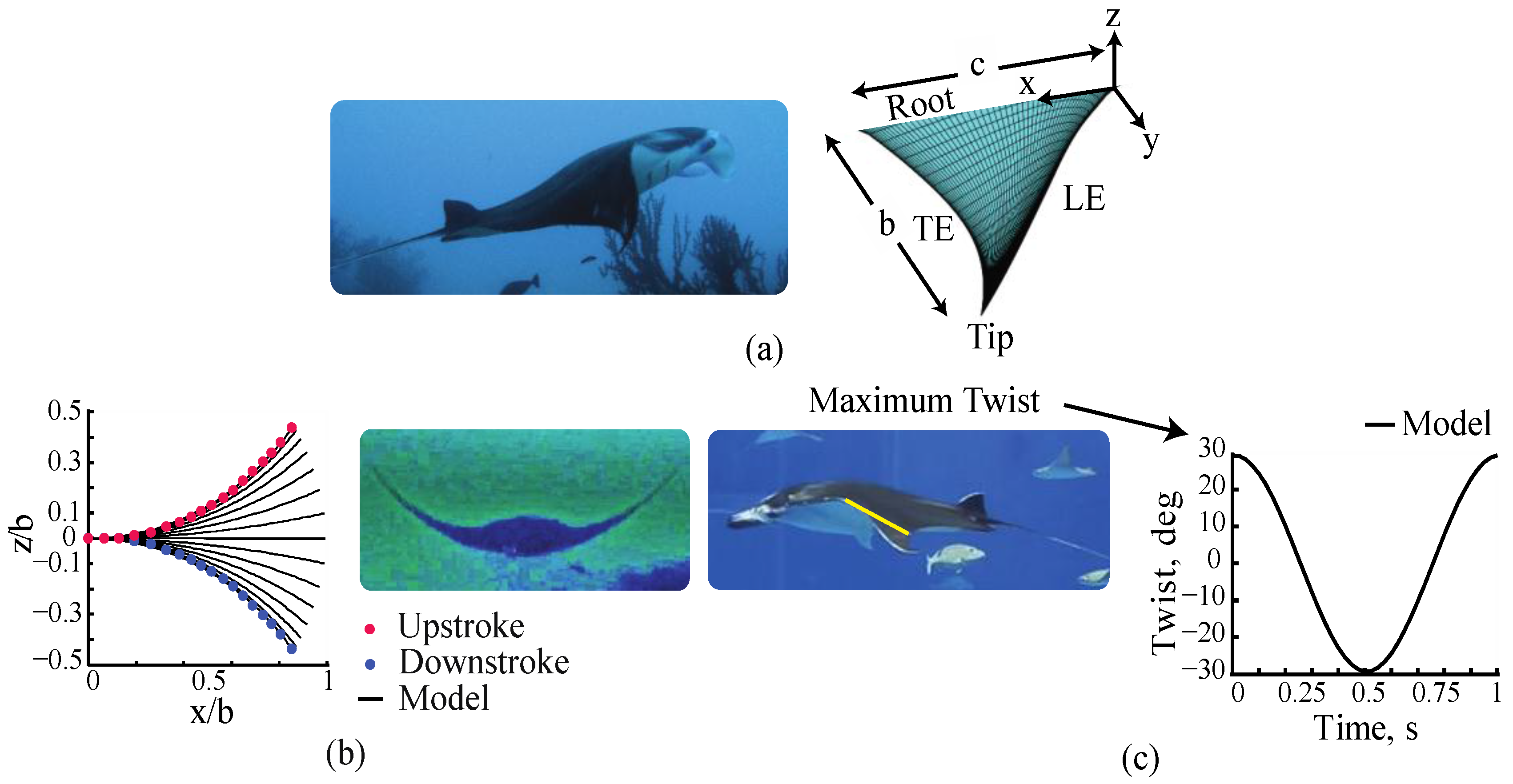
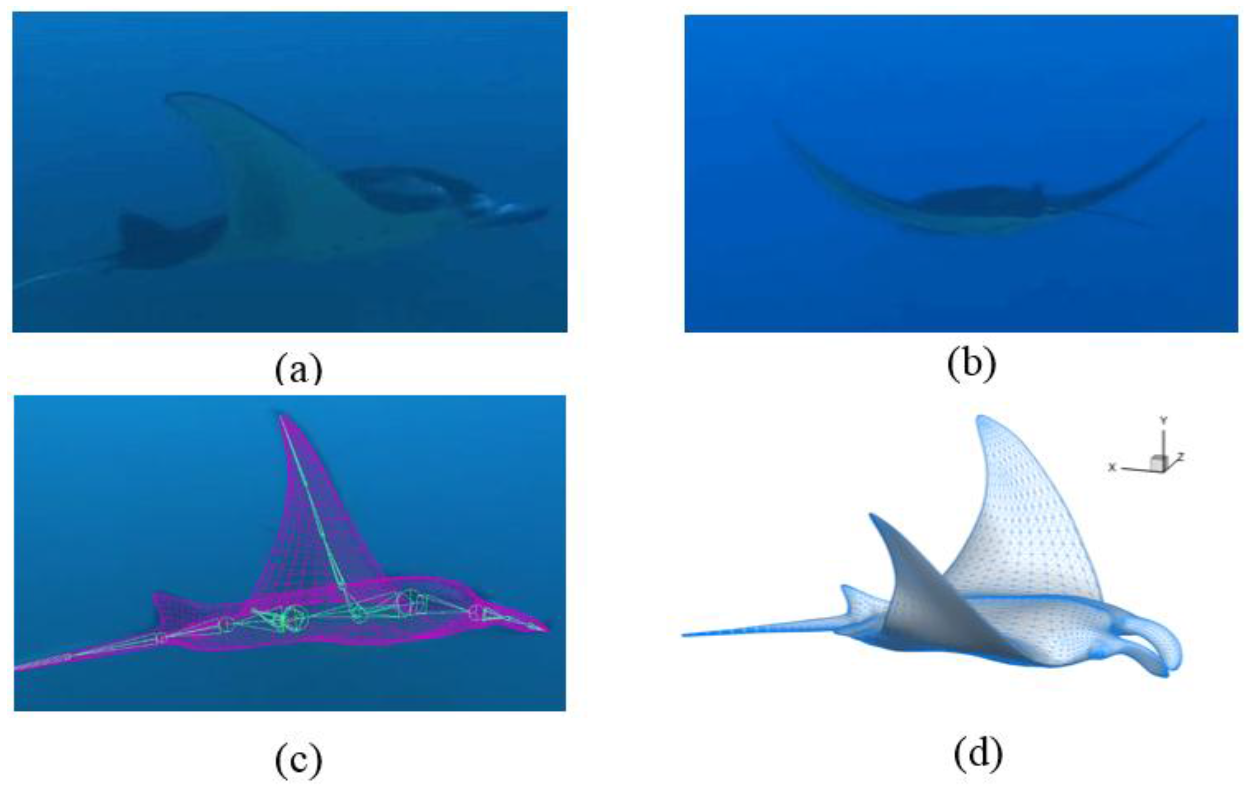
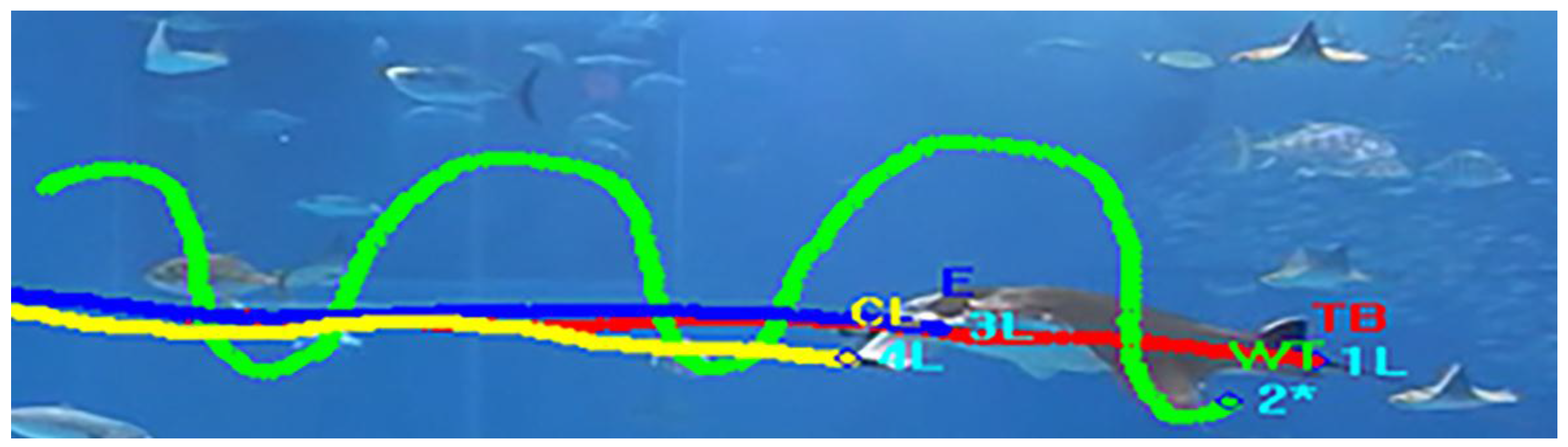
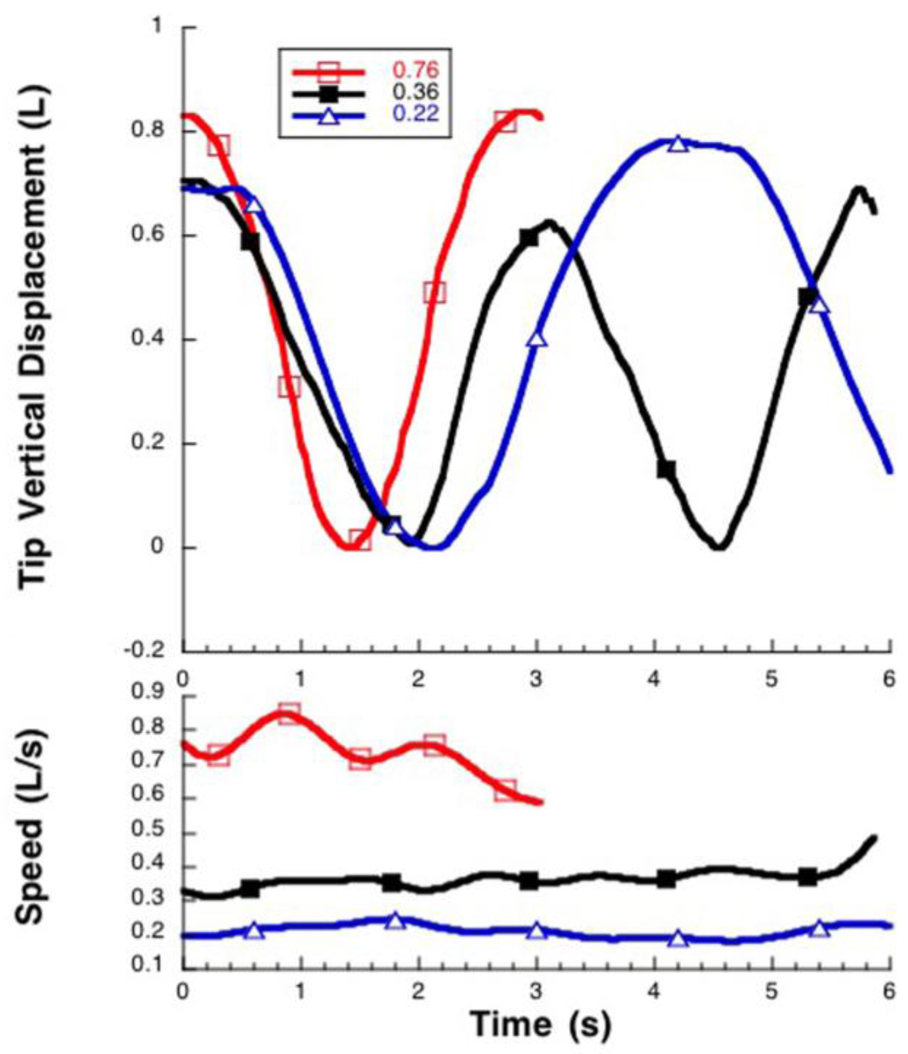
2.1. Manta Kinematics

The swimming performance of nine adult mantas (Manta birostris) was examined in large tanks at the Georgia Aquarium (n = 2), Atlantis Casino and Resort Hotel (n = 2), and Okinawa Churaumi Aquarium (n = 5). As the mantas swam past a large, flat viewing window, lateral views were recorded with a Sony Digital 8 Handycam (HDR SR11, Sony Electronics Inc., San Diego, CA, USA) at 60 Hz. The camera was situated on a tripod at least 7.0 m from the viewing window. The mantas swam freely past the viewing window without interference from the window, the bottom of the tank, and other organisms.

Video records of the swimming mantas were analyzed frame-by-frame using ProAnalyst^® (3-D Professional Ed., v1.5.4.8, Xcitex Inc., Cambridge, MA, USA, 2010) software. Single and multiple stroke cycles were analyzed by manually tracking the manta’s rostrum, tail base, and pectoral fin tip. As each manta was free to swim anywhere in its tank. As no scale could be placed on the animal and the various study sites did not have measurements on the individual mantas, linear distances of each digitized point was scaled relative to the animal’s body length (BL). The digitized data were used to measure relative swimming speed (U_BL; BL/s), stroke frequency (f; Hz; 1/period of stroke cycle) and heave amplitude (A; BL; maximum vertical displacement of pectoral fin tips).

To assess the efficiency of swimming by the manta based on kinematics, the Strouhal number (St) was calculated. The highest propulsive efficiencies for oscillating foils are found at St = 0.25–0.4 [15,16,20,21]. St is related to how fast vortices are being shed into the wake of an oscillating foil and the space between the vortices at each half stroke. St is defined as:

St = Af/U

(1)

where A (m) is the peak-to-peak tip amplitude and U (m/s) is the mean forward velocity. To determine St for a typical manta, BL was scaled as 1.85 m for a manta with a tip-to-tip pectoral fin span of 3.50 m.

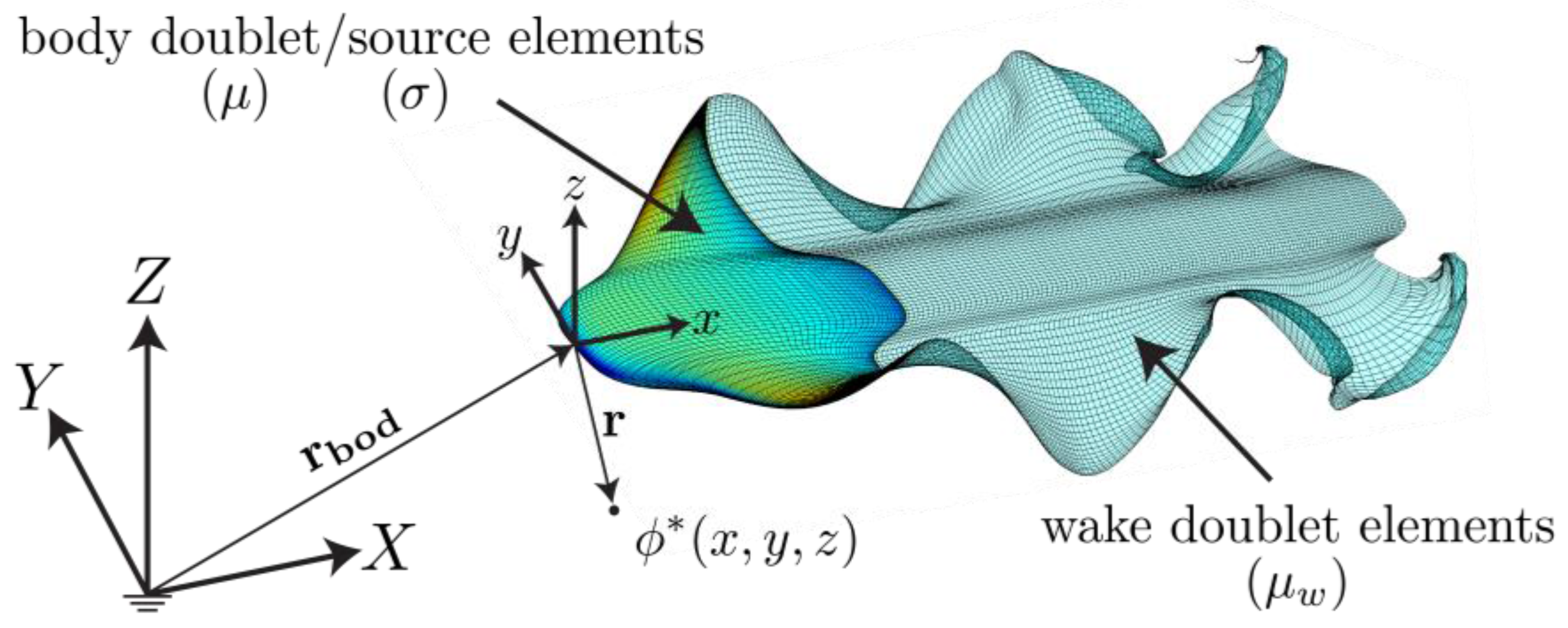
2.2. Potential Flow Model

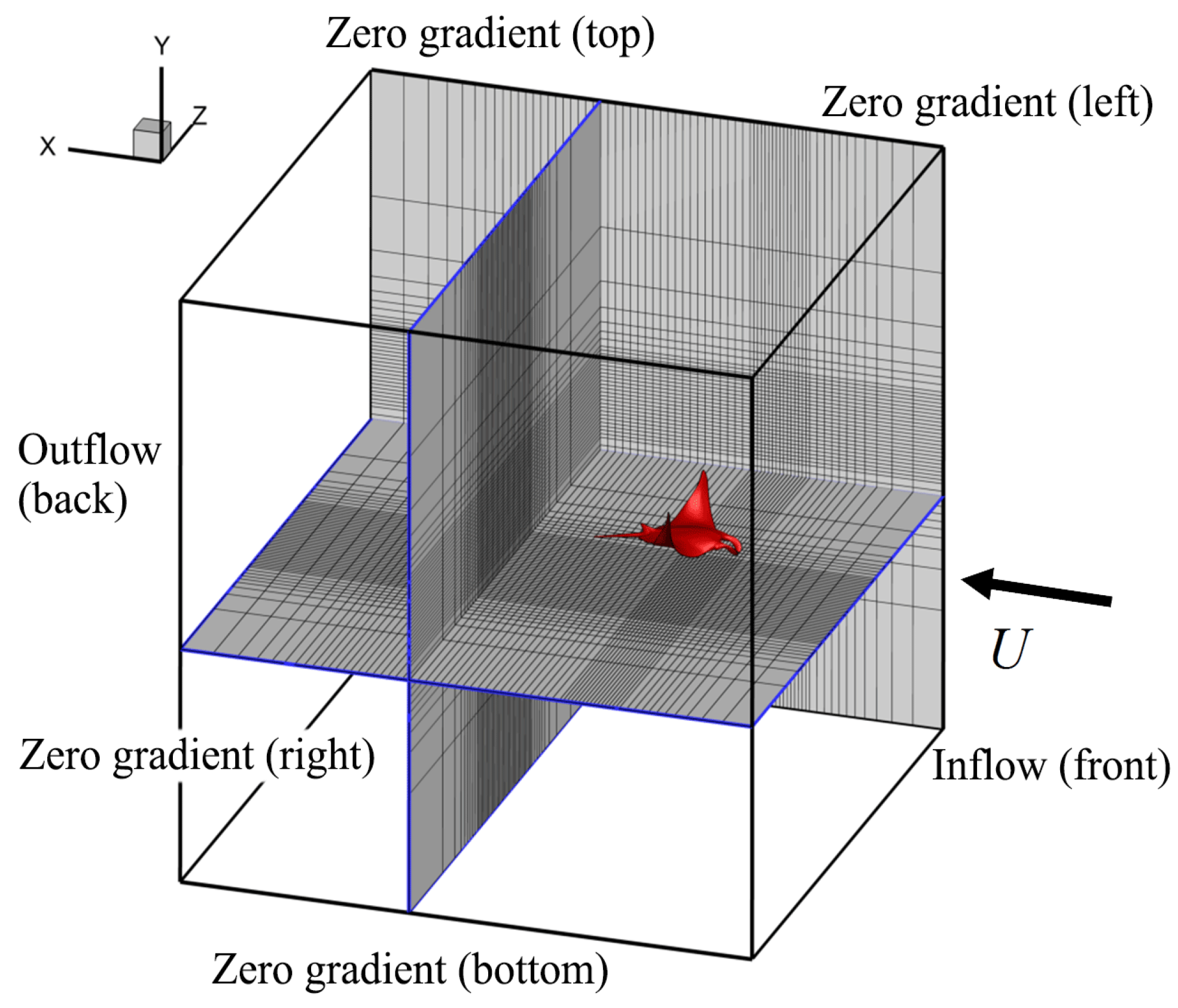
From the acquired video sequences we observed that the motion utilized by rays for rectilinear propulsion can be decomposed into two coupled motions: curved spanwise deformation and a chordwise traveling wave. This observation inspired the development of a mathematical kinematic model that captures these motions into a system of readily implementable equations.

In Figure 1a, a reference coordinate system is given for a generic pectoral fin of a manta ray. The span length, b, is measured from the root to the tip while the chord length, c, is measured from the leading-edge to the trailing-edge at the root of the fin. The root of the fin is defined as the most distal y–z plane, where no fin deformation occurs during a flapping cycle.

An analytical kinematic model is derived by mapping the coordinates of the flat fin to the coordinates of the deformed fin at some time, t. There are three key features that the model captures: curved spanwise deformation, near zero strain in the span direction during deformation and a chordwise traveling wave.

The first feature is observed from posterior images of rays (Figure 1b). These images show that mantas “curl up” their fins creating a curved spanwise deformation as opposed to rotating them at the root. It is assumed that the fin does not stretch during the motion—stretching is energetically unfavorable—so a second constraint enforces that no tensile strain is induced in the spanwise direction as it deforms. This is mathematically described as a length constraint on the neutral axis of the fin during deformation. Finally, a chordwise traveling wave is incorporated to mimic the wing twist exhibited by mantas (Figure 1c). The following form was chosen for the kinematic model that satisfies the mathematical constraints:

$$\begin{array}{l}x\left(x_f,y_f,t\right)=x_f{e}^{-n{x}_f\left|f\left(y_f,t\right)\right|/b} cos\left[m\frac{x_f}{b} f\left(y_{f,}t\right)\right]\\ y\left(x_f,y_f,t\right)= y_f\\ z\left(x_f,y_f,t\right)= x_f e^{-n{x}_f\left|f\left(y_f,t\right)\right|/b} sin\left[m\frac{x_f}{b} f\left(y_{f,}t\right)\right]\\ \phantom{z\left(x_f,y_f,t\right)}f\left(y_f,t\right)=sin\left(\omega t+K{y}_f/b\right)\end{array}$$

(2)

This description of manta fin kinematics references the coordinate system in Figure 1a. In this formulation, a set of points $\left(x_f,y_f\right)$ defines the neutral plane of a ray fin in a flat position. The model solves for the deformed coordinates $\left(x,y,z\right)$ of the fin at a time, $t$. The time variation was represented as a sinusoidal signal with an angular frequency, $\omega$. The non-dimensional wavenumber is defined as $K=2\pi b/\lambda$ where $\lambda$ is the wavelength of the traveling undulatory wave. The model has four fitting parameters $\left(K,m,n,\omega \right)$. Two $\left(K,m\right)$ are used to fit the biological data extracted from two-dimensional images. The third $\left(\omega \right)$ is used to match the oscillation frequency. The last $\left(n\right)$ is used to minimize the strain in the span direction during large-amplitude deformation and an optimal choice of $n=0.1342 m^2$ is used. For the manta, the strain was minimized to under 1% for the entire deformation.

The first biological fitting parameter, $m$, is directly related to the dorso-ventral amplitude of motion along the span.

$$A\left(x_f\right)=x_f{e}^{-0.1342m^2{x}_f/b}\sin \left(m{x}_f/b\right)$$

(3)

The non-dimensional tip amplitude can be used to solve the nonlinear equation for $m$, that is, $e^{-0.1342m^2{x}_f/b}\sin \left(m\right)=A/b$. By solving this equation a value of $m=0.4807$ was determined for the manta. This ensured a good match between the model and the actual kinematics along the entire span as seen in Figure 1b.

The second biological fitting parameter, $K$, was determined by extracting the maximum twist angle, ${\theta }_{max}$, of a ray wing at a given spanwise location (Figure 1c). The non-dimensional wavenumber is calculated from the amplitude (Equation (3)) and the extracted angle as,

$$K={\theta }_{max}/\left[A\left(x_f\right)/b\right]$$

(4)

The data for the maximum twist angle and the span location are approximated from a single lateral picture of the animal (Figure 1c). A maximum twist angle of ${30}^{\mathrm{o}}$ at the $3/4$ span was estimated and a value of $K=2.23$ was determined to match well with the lateral images of the animal.

The kinematic model was coupled with an idealized geometry of a manta and it was used with a boundary element method (BEM) to calculate the fluid flow around a free-swimming manta. The boundary element method is a potential flow method for unsteady, three-dimensional flows where the flow is assumed to be irrotational (except on the elements), incompressible, and inviscid. For free-swimming, we define the problem in an inertial frame of reference that is attached to the undisturbed fluid (Figure 2). As such the velocity field, $\mathit{u}$, may be defined everywhere as the gradient of a scalar velocity potential, that is, $\mathit{u}=\mathbf{\nabla }{\varphi }^{*}$, where ${\varphi }^{*}$ is the perturbation potential defined in the inertial frame with zero free-stream velocity. Once the perturbation potential is determined, the velocity field may be determined and in turn the pressure field acting on the body may be calculated by using the unsteady Bernoulli equation cast in the body-fixed frame of reference,

$$P\left(x,y,z,t\right)=-\rho {\frac{\partial {\varphi }^{*}}{\partial t}|}_{\text{body}}+\mathsf{\rho }\left(u_{rel}+U_{bod}\right)·\mathbf{\nabla }{\varphi }^{*}-\mathsf{\rho }\frac{{\left(\mathbf{\nabla }{\varphi }^{*}\right)}^2}{2}$$

(5)

The problem is then reduced to solving Laplace’s equation for the perturbation potential throughout the fluid,

$${\nabla }^2{\varphi }^{*}=0$$

(6)

The boundary conditions that must be satisfied for an inviscid fluid are that there is no fluid flux through the body surface and that the flow disturbances caused by the body must decay far away,

$$\begin{array}{c}\widehat{\mathit{n}}·\mathbf{\nabla }{\varphi }^{*}=\widehat{\mathit{n}}·\left({\mathit{u}}_{\mathit{r}\mathit{e}\mathit{l}}+{\mathit{U}}_{\mathit{b}\mathit{o}\mathit{d}}\right) on S_b\\ {\mathbf{\nabla }{\varphi }^{*}|}_{r\to \infty }=0 on S_{\infty }\end{array}$$

(7)

The body surface is denoted as $S_b$, the surface at infinity bounding the fluid domain is $S_{\infty }$ with $\mathit{r}={\left[x, y, z\right]}^T$, the outward normal vector from the body surface is $\widehat{\mathit{n}}$, the instantaneous translational speed of the body-fixed frame of reference is ${\mathit{U}}_{\mathit{b}\mathit{o}\mathit{d}}$, and the velocity of the body surface within the body-fixed frame of reference is ${\mathit{u}}_{\mathit{r}\mathit{e}\mathit{l}}$.

Following Katz and Plotkin [22], a general solution to this potential flow problem is reduced to finding a distribution of doublets and sources on the body surface and in the wake that satisfied the no flux boundary condition on the body at each time step. The elementary solutions of a doublet and source both implicitly satisfied the far-field boundary condition. The Dirichlet formulation is used to satisfy the no-flux condition on the body where,

$$\begin{array}{c}-\mu ={\varphi }^{*}\\ \sigma =\widehat{\mathit{n}}·\left({\mathit{u}}_{\mathit{r}\mathit{e}\mathit{l}}+{\mathit{U}}_{\mathit{b}\mathit{o}\mathit{d}}\right)\end{array}$$

(8)

Here, the strength of the unknown doublet distribution locally is $\mu$ while the strength of the known source distribution locally is $\sigma$. To solve this problem for ${\varphi }^{*}$ numerically, the singularity distributions are discretized into constant strength quadrilateral boundary elements over the body and wake. Thus, a linear system of equations must be solved,

$$\begin{array}{c}{\displaystyle \sum _{j=1}^{N_b}}{A}_{ij}{\mu }_j=-{\displaystyle \sum _{j=1}^{N_b}}{B}_{ij}{\sigma }_j-{\displaystyle \sum _{k=2}^{N_w}}{C}_{w,ik}{\mu }_{w,k}\\ \mathrm{with}\\ \begin{array}{cc}{A}_{ij}=& \{\begin{array}{c}{C}_{ij}-C_{w,i1}, j=\mathrm{bottom}\mathrm{element}\\ C_{ij}+C_{w,i1}, j=\mathrm{top}\mathrm{element}\\ C_{ij} \text{otherwise}\end{array}\end{array}\\ \mathrm{and}\\ B_{ij}= -\frac{1}{4\pi }{{\displaystyle \int }}^{\text{}}\frac{1}{\left|\mathit{r}\right|} \mathrm{d}{S}_0\\ C_{ij}= -\frac{1}{4\pi }{{\displaystyle \int }}^{\text{}}\frac{\widehat{\mathit{n}}·\mathit{r}}{{\left|r\right|}^3} \mathrm{d}{S}_0\\ C_{w,ik}= -\frac{1}{4\pi }{{\displaystyle \int }}^{\text{}}\frac{\widehat{\mathit{n}}·\mathit{r}}{{\left|r\right|}^3} \mathrm{d}{S}_0\end{array}$$

(9)

for the unknown doublet distribution. Here, $N_b$ is the number of body elements, $N_w$ is the number of wake elements, $\mathit{r}$ is the position vector from the element to a point of interest, and the influence matrices, $C_{ij}, B_{ij}, C_{w,ik}$, are integrated over the surface of a boundary element. The conditional statement for the influence matrix, $A_{ij}$, is the implementation of an explicit Kutta condition, which serves to set the circulation around a spanwise station such that there is a stagnation point at the trailing-edge [23,24]. These boundary elements produce an irrotational flow field everywhere except on the elements themselves. As such, these elements serve to model the vorticity in the flow, which is generated on the body and shed to form the wake. At each time step a wake boundary element is shed with a strength that is set by applying the explicit Kutta condition at the trailing edge.

At every time step, the wake elements advect with the local velocity field such that the wake does not support any forces. During this wake rollup, the perimeter of the wake doublet elements, which are line vortices, are de-singularized for the numerical stability of the solution [25]. A desingularized Biot–Savart law was used to calculate the wake deformation [24]. That is, the corner points of the wake quadrilateral elements are displaced by $\mathit{u}\left(\mathit{x}\right)\Delta t$ where,

$$\mathit{u}\left(\mathit{x}\right)=\frac{\Gamma }{4\pi }{{\displaystyle \oint }}^{\text{}}\frac{\mathit{s} \times \mathit{r}}{r^3+{\delta }^3} ds$$

(10)

and $\Delta t$ is the time step. The wake doublet elements are equivalent to a wake vortex ring element with the perimeter of the element being a series of line vortices of strength, $\Gamma = -\mu$. The length along the perimeter is $s$ and the desigularization parameter is $\delta$.

The tangential perturbation velocity over the body, that is the velocity due to the perturbation potential, was found by a local differentiation of the perturbation potential by using a fourth-order finite difference scheme. The unsteady Bernoulli equation was then used to calculate the pressure acting on the body (see Equation (5)).

The shear stress acting on the body was estimated through the use of a one-way coupled boundary layer solver. The computational model was broken up along the span into a series of chordwise strips for the boundary layer analysis. The outer potential flow over the body was used in conjunction with the stagnation point location on a strip to determine the laminar boundary layer properties via the method of Thwaites [26]. Transition to a turbulent boundary layer was predicted by using the correlation function proposed by Cebeci and Smith [27] for the “e⁹” method. The turbulent boundary layer properties were then determined via a momentum integral analysis assuming a 1/7-power velocity profile [22]. Using this boundary layer solver gave the skin friction drag over the body from both the laminar and turbulent portions of the boundary layer; however, this did not include the effect of mild trailing-edge separation that led to form drag. Form drag was estimated by determining the local angle of attack on each strip and the local frontal area, which was used to modify the skin friction drag coefficient for each strip.

The pressure and shear stress was then integrated over the body surface to calculate the forces and moments acting on the body. These streamwise forces were used to solve for the dynamics of free-swimming, where the streamwise degree of freedom of the body was unconstrained and the cross-stream and rotational degrees of freedom were all constrained.

Figure 3 shows the grid and time step sensitivity of the BEM model. In this convergence study, the mantas were free-swimming for three flapping cycles. The frequency of fin oscillation was $f=0.5$ Hz and the initial velocity of the rays was $U_0=0.06$ m/s. The cycle-averaged speed, $\overline{U}$, and swimming economy, $\xi =\overline{U}/ \overline{P}$, changed by less than 1% and when the number of body panels $N=6400$ and the number of times steps per flapping cycle $N_{step}=60$ were doubled.

The BEM computations in the following sections were all started at a near zero velocity of $U_0=0.05f$ m/s. The solution was computed for twelve flapping cycles and the time-averaged data were obtained by averaging over the last cycle. All forces are reported as force coefficients where they are normalized by a characteristic force $1/2\rho {\overline{U}}^2 S$. The fluid density is $\rho$, the ray planform area is $S$, and the cycle-averaged swimming speed at steady state is $\overline{U}$. For the BEM solution, an idealized manta ray was modeled that had a body length of $L=1.97$ m, a tip-to-tip span of $2b=3.751 m$ where b is the half-span. The geometry differs from the viscous model (see below) since the BEM solver is constructed to accept parametrically defined geometries instead of the direct import of point-cloud geometries. By using triangular higher-order elements this feature may be changed [23].

2.3. Viscous Model

Based on the lateral view (Figure 4a) and rear view (Figure 4b) images of steady swimming by the manta, a virtual skeleton-based 3D surface reconstruction method was used to obtain the morphing fin kinematics of the swimming manta. As shown in Figure 4c, the manta’s pectoral fins were bounded with a series of virtual skeletons that were connected one after another and could be rotated about their joints with three degrees of freedom. At each time, we adjusted the rotating angles of those skeletons to match our models with the images. Finally, the surfaces of the reconstructed model were represented by triangular cells (Figure 4d). This method was developed from the previous marker-based 3D surface reconstruction of insect flight [28] and its accuracy has been evaluated by comparing the positions of the fin tip, leading edge and trailing edge between the model and the experimental data.

The reconstructed models were then imported as immersed moving boundaries in our in-house immersed-boundary-method-based computational fluid dynamics (CFD) solver. The numerical methodology employed in the current study is briefly introduced as the following. The 3D incompressible Navier–Stokes equations were discretized using a cell-centered, collocated arrangement of the primitive variables, and was solved using a finite difference-based Cartesian grid immersed boundary method [29]. The immersed-boundary treatment is the same as that in Dong et al. [30]. The equations were integrated in time using the fractional step method, which consists of three-steps. In the first sub-step of this method, a modified momentum equation is solved. A second-order, Adams–Bashforth scheme is employed for the convective terms while the diffusion terms are discretized using an implicit Crank–Nicolson scheme which eliminates the viscous stability constraint. A second-order central difference scheme was employed in space discretization. This method was successfully applied in many simulations of flapping propulsion [31,32,33]. More details about this method can be found in [29,30]. Validations about this solver can be found in our previous works [32,34].

According to the biological data, the Reynolds number of manta swimming ranges from $6.85\times {10}^5$ to $7.71\times {10}^6$ (see Section 3.1 below), which indicates that the flow is fully dominated by the inertia effect. This is too high to be directly simulated by current computational capability. On the other hand, the purpose of the viscous flow simulation was to capture the key features of the wake structures for addressing the fundamental hydrodynamic mechanisms of a manta-like model’s swimming. Previous studies [35,36] have shown that the major flow features are similar in flapping propulsion with changing of the Reynolds number. In order to understand the predominant vortex dynamics features, the Reynolds number in current viscous flow simulation has been set to 1200, at which the inertia is still more significant than viscosity, for meeting the requirement of the mesh resolution and computational cost by the simulation of swimming objects. This is equivalent to a smaller size body performing a slower motion. According to the stability requirements of the flow solver, the time step was chosen to be T/960, where T is the period of the flapping motion.

The simulations were carried out on a non-uniform Cartesian grid (Figure 5). The computational domain size was chosen as $30\times 30\times 30$ (normalized by BL) with $272\times 160\times 224$ (about 9.7 millions) grid points in total. A cuboidal region around the manta with high-resolution uniform grids with the spacing of about 0.01 is designed to resolve the near-field vortex structures. This mesh setup was based on a grid-independent study, in which the mean force coefficients differ by less than 1.5% between the current grid and a finer grid (with 298 $\times$ 174 $\times$ 44 = 12.7 millions grid points). The boundary condition set-up is same as [30]. At the right-hand boundary, we provided a constant inflow velocity boundary condition. The left-hand boundary was the outflow boundary, and there we provide a zero streamwise gradient boundary condition for velocity which allows vortices to convect out of this boundary without significant reflections. The zero gradient boundary condition was applied at all lateral boundaries. A homogeneous Neumann boundary condition was used for the pressure at all boundaries. To study the long-term hydrodynamic performance of the flapping fins in steady swimming, a uniform flow of speed U passing the tethered manta model was utilized to save on computation cost. U was set as 1 body length per flapping cycle, which corresponds to 0.3 BL/s at the flapping frequency 0.3 Hz. According to observations of swimming mantas (below), this speed is within the range of the experimental observation. To ensure the convergence of the flow, a criterion of ${10}^{-6}$ for the velocity was used. About 84 CPU hours on a single Intel^® Core™ i7-3770 CPU@ 3.4 GHz computer node were generally needed. Results presented here were obtained by simulating the flow over five fin strokes.

3. Results

3.1. Manta Kinematics

A total of 152 swimming sequences for the nine mantas were analyzed. Mantas swam by exclusively flapping their expanded pectoral fins in the vertical plane through and upstroke and downstroke (Figure 6 and Figure 7). The stroke was dorsoventrally asymmetrical with a gliding phase at the top of the stroke particularly at slow swimming speed (Figure 7 and Figure 8). This asymmetry produced oscillations in swimming speed. In addition, the fin tips were abducted higher over the longitudinal axis of the body than adducted under the body. Both spanwise and chordwise flexibility were apparent as the pectoral fins were oscillated. Initiation of both upstroke and downstroke occurred at the anterior base of the fin (Figure 6) and proceeded movement of the fin tip in the same direction. These actions resulted in a wave moving spanwise through the fin from fin base to tip with less than one full wavelength. Another wave of longer wavelength was directed chordwise through the fin. Flexibility in the fin also produced twisting toward the fin tip during the upstroke (Figure 6; 2.1 s). Detailed kinematic features of the fin flapping based on a high-resolution reconstruction was presented in Section 3.2.

The frequency (f) of oscillation of the pectoral fins increased directly with increasing swimming speed (Figure 9a), according to the equation:

f = 0.189 + 0.223 U_BL

(11)

which was statistically significant (r = 0.589; p < 0.001; degrees of freedom (d.f.) = 150). The heave amplitude (A) did not demonstrate a statistically significant change with U_BL (Figure 9b; r = 0.154; p < 0.0579; d.f. = 150). The mean ± one standard deviation (SD) for A was 0.824 ± 0.225 BL.

Over a range of U_BL of 0.2 to 2.25 BL/s, the calculated U ranged from 0.37 to 4.16 m/s, based on a typical manta with BL = 1.85 m. Based on this BL, the amplitude of heave averaged 1.43 m. This range in speeds indicated that mantas would be swimming with a Reynolds number of 685,240 to 7,708,952. The Strouhal number (St) decreased asymptotically with increasing U_BL (Figure 10). At U_BL of 0.2 BL/s, St was 0.96, but decreased to 0.25 at U_BL of 2.25 BL/s. U_BL of approximately 0.72 BL/s represented the crossover point at which St moved into the optimal range of 0.2 to 0.4, where propulsive efficiency is considered to be maximal. All values >U_BL of 0.72 BL/s were within the optimal range of St.

3.2. Potential Flow Model

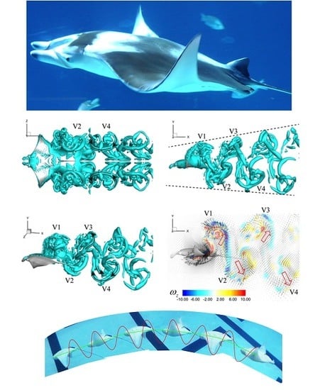
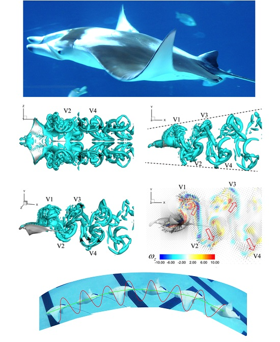
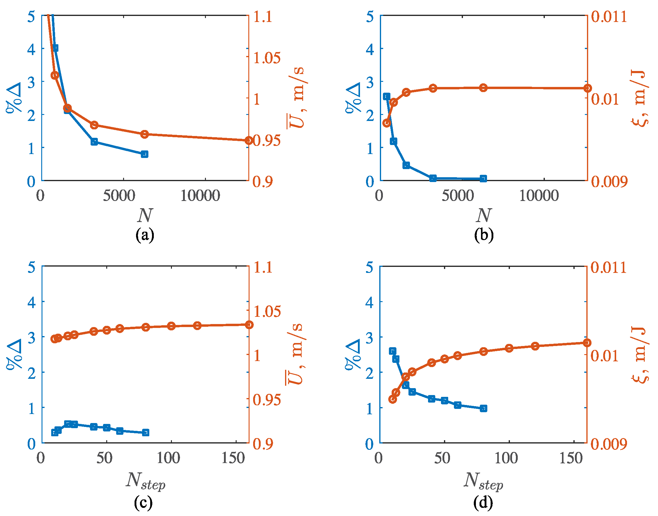
All of the computations using the BEM were at a free-swimming condition, where the net thrust coefficient was $C_{T,net}=O\left({10}^{-4}\right)$. The net thrust coefficient was the net time-averaged thrust force ${\overline{T}}_{net}$ non-dimensionalized by the characteristic force described earlier. Figure 11a shows the swimming speed as a function of time for rays swimming with different oscillation frequencies. Going from blue to red the frequencies range from 0.1 to 0.6 Hz, respectively. The simulations were started near zero velocity and the rays were allowed to accelerate until a cycle-averaged steady-state condition occurred around 12 swimming cycles. The acceleration of the rays was seen to scale up with increasing frequency. In addition, at the highest frequency of 0.6 Hz the surging of the ray is clearly observed when a trailing-edge vortex structure is shed. The other frequencies exhibit these surging oscillations albeit with a smaller amplitude.

When the steady-state of the cycle-averaged velocity is plotted, there was a near linear increase in speed with an increase in the oscillation frequency as seen in Figure 11b (left axis). The numerical data is also in excellent agreement with the biological data from Figure 9a, which is superimposed for a direct comparison. The right vertical axis shows that when the steady-state of the cycle-averaged swimming speed is non-dimensionalized by $fL$, where $L$ is the body length of the manta, the velocities collapse to a constant value of about 1.5 body lengths per flapping cycle highlighting the near linear trend with frequency.

The left axis of Figure 12a shows the St number as a function of the swimming speed normalized by the ray body length. The inverse trend in St with swimming speed observed from the biological measurements was also seen in our computational data. Indeed, the propulsive efficiency tends to a high value of about 89% as the St asymptotes (Figure 12a, right axis). The propulsive efficiency is defined as:

$$\eta = \frac{\overline{T}\overline{U}}{{\overline{P}}_{in}}$$

(12)

where $\overline{T}$ is the time-averaged thrust force calculated as the streamwise directed pressure forces and ${\overline{P}}_{in}$ is the time-averaged power input to the fluid. ${\overline{P}}_{in}$ is calculated as the negative inner product of the force vector and the velocity vector of each boundary element. There are other energetic metrics discussed throughout the literature. One is the cost of transport (CoT), which first made its appearance in an article from Gabreilli and von Kármán [37] as the tractive force to weight ratio. The cost of transport is a measure of the amount of energy it takes to travel a unit distance per unit mass. This is the inverse of a “miles-per-gallon” economy calculation that is reported on a per-unit-mass basis. It is calculated as:

$$CoT= \frac{{\overline{P}}_{in}}{M\overline{U}}$$

(13)

where M is the mass of the manta ray, which in the BEM computations was taken to be $M=450$ kg. This energetic metric is used throughout biological literature [38]. From Figure 12b (left axis) the CoT is seen to increase with increasing swimming speed. This highlights that even though the efficiency is nearly constant with increasing swimming speed, the amount of energy to travel a given distance is increasing. Therefore, more power is required to swim faster with the same efficiency. CoT can be non-dimensionalized with a characteristic drag force and the body mass as:

$$Co{T}^{*}=\frac{CoT M}{1/2\rho {\overline{U}}^{2}S}$$

(14)

The solid line with triangle markers in Figure 12b shows that CoT* is nearly a constant value (plotted on the left axis) and in fact it reflects an inverse relationship with efficiency. The CoT* is readily measurable for free-swimming devices by measuring power input and swimming speed and for animals by measuring their oxygen consumption; however, to estimate the propulsive efficiency, $\eta$, the three-dimensional time-varying flowfield must be quantified [39]. The CoT* offers a new non-dimensional approach to calculating a free-swimming efficiency-like metric. On the right axis of Figure 12b, the Froude efficiency is plotted as defined by Tytell and Lauder [40]. Here the Froude efficiency is:

$${\eta }_f= \frac{\overline{T}\overline{U}}{\overline{T}\overline{U}+{\overline{P}}_{lat}}$$

(15)

where ${\overline{P}}_{lat}$ is the power input laterally to the fluid that is only in the cross-stream directions.

The single case of $f=0.3$ Hz was analyzed in detail. For these results the initial swimming speed was near the cycle-averaged steady-state swimming speed and only four flapping cycles were calculated. Figure 13a,b,d shows the vortex wake produced by a free-swimming manta ray. The vortices are marked as isosurfaces of the ${\lambda }_2$ criteria, which distinguishes pressure minima in a plane after discarding unsteady straining and viscous effects [41]. The manta is seen to shed a series of interlocked vortex rings with one set originating from each pectoral fin. The vortex rings induce a velocity field through their centers, which when the x-component is time-averaged is seen in Figure 13c. Here three isosurfaces of velocity are shown at 1%, 1.5% and 2% above the steady-state of the cycle-averaged swimming speed. The flow is seen to speed up in the x-direction over the body of the ray and in two distinct velocity jets aligned with the centers of the vortex rings.

The velocity jets are indicative of thrust production because the force to cause a momentum change of the fluid is accompanied by an equal and opposite force acting on the body. This force was reflected in the pressure field acting over the body presented (Figure 14a). The pressure is reported as the time-averaged coefficient of pressure, $C_P=P_{body}/\left(1/2\rho {\overline{U}}^2\right)$, where the pressure over the body is taken to be gage pressure. As the flow accelerates around the leading edge of the body and fins, the pressure drops causing leading-edge suction and some concurrent thrust force. The strength of leading-edge suction was seen to be greater over the fin region than the body region. In fact, the body also displayed a large area of near stagnation pressure at its leading edge marked by blue.

The time-averaged skin friction coefficient is calculated as $C_f=\tau /\left(1/2\rho {\overline{U}}^2\right)$ (Figure 14b). The boundary layer flow is initially laminar starting at the stagnation point and the skin friction increased as the flow accelerates around the leading edge. Then the skin friction decreased as the flow slows down due to the adverse pressure gradient over the top of the ray. Around halfway down the length of the ray, the boundary layer transitions to a turbulent boundary layer. The skin friction jumps up and then continues to slowly decrease as the flow slows down approaching the trailing-edge stagnation point.

The time-varying contributions to the force production are distinguished as the pressure forces acting on the fins and body and the shear forces acting on the fins and body (Figure 14c). The estimate of the form drag pressure force was nearly zero and acts solely on the fins. The pressure force on the fin is the only contributor to thrust production. The shear force on both the fins and body is seen to incur a drag penalty. Surprisingly the pressure force acting on the body is non-zero and drag producing. This is unexpected since the body stayed fixed at zero pitch and did not include any leading-edge separation models. For potential flow solutions without leading-edge separation models, drag due to pressure forces is produced through the reorientation of the lift vector from induced downwash or upwash. Thus, it was concluded that this pressure-based drag force must be an induced drag force due to the wake vortex system.

When the various force contributions were integrated over a chordwise strip the thrust producing and drag producing regions of the ray could be distinguished (Figure 14d). The net time-averaged force in the x-direction is non-dimensionalized with a characteristic force defined earlier. From the center of the body at 0.48 of the half-span, b, the ray body switches from net drag production to net thrust production. This transition location is in excellent agreement with the viscous model, which found the transition to occur at 0.46b from the center of the body.

The induced drag force on the body is a surprising result (Figure 14c). The vertical velocity component, w, is shown along the z = 0 plane in the wake of the ray (Figure 15a). As expected, there are regions of upwash and downwash associated with the vortex ring system. What is unexpected is that in the central region where the body travels there are also oscillating regions of upwash and downwash. Because the pitch angle of the body was fixed in the simulations, the regions of upwash and downwash over the body induced an angle of attack, which in turn induced a drag on the body.

These results are reflected in the root-mean-squared (rms) circulation distribution (Figure 15b). At the center of the body, the rms circulation is seen to be non-zero, which means that there is at least time-varying lift production and there is concurrent time-varying induced drag. It is also observed that the maximum downwash over the body region occurs when the fins flap downward near the point where they pass through the z = 0 plane (Figure 15a). To counteract the induced angle of attack, which in this case was downward, the ray needs to pitch up by a small amount. By doing so they could reduce their effective angle of attack and minimize the induced drag acting on their body. Indeed, the body kinematics of mantas shows that they do pitch up during their downstroke and pitch down during their upstroke. It is postulated that this reduces their induced drag and increases their propulsive efficiency. Mantas could simply do this without active control by being unstable in pitch; therefore, in this case, their center of mass would be behind their time-averaged center of pressure.

3.3. Viscous Model

A series of snapshots of our reconstructed model is shown in Figure 16. And the detailed flapping kinematics of the pectoral fin in this model was analyzed during downstroke and upstroke, (Figure 17). According to the tip trajectory (Figure 17a, red line), the distal part of the pectoral fin had a forward flapping component relative to the body in the early stage of the downstroke right after the reversal. It also had a backward component during the upstroke, which was like a paddling motion. The fin tip (point 5 in Figure 17b2) showed the largest flapping amplitude (about 1.05 BL). The flapping motion during downstroke was faster than during upstroke because the duration of the downstroke was only 0.43 T, which is shorter than that of upstroke (0.57 T). The displacement peaks of different marker points happened at different time instants, and the outer markers always lagged behind the inner markers. These displacements demonstrated that there was a travelling wave propagating from the root to the tip when the pectoral fins were flapping. The pitching angles reached the maximum at the mid-downstroke and after the reversal in upstroke (Figure 17). The pitching amplitude of the distal part (0.85 half-span) of the fin reached as high as 70° (Figure 17c2). This displacement of the distal fin was about 2.5 times the pitching amplitude of the root region (0.3 half-span). The pitching angle distribution along the span indicated that there was a significant twist on the fin.

Forces were computed through direct integration of the surface pressure/shear as described by Ghias et al. [42]. To better understand the thrust producing mechanism, the force components were examined for the pressure force and the shear force along the swimming direction, which were considered as thrust (F_T, opposite to x-direction) and drag (F_D, along x-direction), respectively. The coefficients C_T and C_D were obtained using (C_T, C_D) = (T, D)/0.5ρU²BL² with ρ as the density of water. The coefficient of the resultant force along the forward direction of manta was denoted by C_X = C_T – C_D. There was temporal variation of C_T, C_D and C_X over one cycle when the simulations reached a periodic state, and a number of observations were made regarding these plots (Figure 18).

Table 1. Cycle-averaged values of force coefficients.

$\overline{{\mathit{C}}_{\mathit{T}}}$	$\overline{{\mathit{C}}_{\mathit{D}}}$	$\overline{{\mathit{C}}_{\mathit{X}}}$
0.111	0.097	0.014

shows the mean values ($\overline{C_T}$, $\overline{C_D}$, and $\overline{C_X}$) of force coefficients over the last two flapping cycles.

It was noted that both downstroke and upstroke produced peaks in thrust force. The peak in the downstroke was about 0.55, which was 1.41 times the peak in the upstroke. The difference of peaks in force was attributed to the higher flapping speed in the downstroke. Positive C_T happened when the pectoral fin flapping speed was relatively high (see the slope of the tip displacement), while negative C_T appeared during the stroke reversals. In addition, the peak in C_T during downstroke appeared near the moment as the pitching angle exhibit peak value. The above analysis suggested that the thrust production was correlated with both the flapping and the pitching of the pectoral fin. The viscous drag (C_D) seemed to be minimally affected by the fin flapping, because variation of C_D was much smaller than that of C_T. The cycle-averaged value of C_T is 0.111, which was slightly higher than the absolute value of cycle-averaged C_D (0.097). This indicated that the simulation setup was close to steady swimming.

The contribution to thrust production from different portions of the fins was examined by the local distribution of $\overline{C_X}$ over a flapping cycle on the model surface (Figure 18b). The dashed line located at about 0.46 half-span (consistent with that in the potential flow model) away from the middle of the body indicates the separation point between the thrust production and drag production of the manta model. The red region ($\overline{C_X}$ > 0.15) is about 0.68 half-span away from the middle of the body. This indicates that the distal part of the fin plays the most important role in thrust production. Both the body and the basal part of the fin experiences drag, but the magnitude of this drag (blue, no less than 0.05) is much smaller than for the thrust (red, higher than 0.15) on the distal part of the fin. This difference is because the distal part of the pectoral fin has higher flapping amplitude (>0.6 BL) and pitching amplitude (>40°), while the body is rigid and remained stationary in the simulation. At the same time, the basal part of the fin has minimal oscillation and chordwise pitching.

To further understand the thrust producing mechanism of manta fins, details on the wake topology and vortex dynamics are analyzed. The flow patterns of a manta model’s swimming had been briefly introduced previously [43]. The 3D vortex structures are visualized by the isosurface of the imaginary part of the complex eigenvalue ($\lambda$) derived from the instantaneous velocity gradient tensor, which identifies flow regions where rotation dominates over strain [44].

During each downstroke or upstroke, there is a vortex ring shed from the trailing edge of the fin, leaving two sets of inter-connected vortex rings in the wake, which are from V1 to V4 following the shedding order (Figure 19). Because the flapping motions of the left pectoral fin and the right one are symmetric, the flow induced by those fins exhibited strict symmetry with respect to the mid-plane of the body (see Figure 19a). The overall structure of the wake is different than the wake of a pitching-plunging plate [30] in which clear circular vortex loops were found. The wake in the present study is similar to the wake of a pitching-rolling plate [45] in which vortex rings are tilted more or less with sub-structures connecting them.

The shape of the vortex rings (V1 and V3) generated by the upstroke flapping is more complex than those (V2 and V4) generated by the downstroke flapping (Figure 19). There are some smaller vortex tubes entangled with V1 and V3. Vortices generated by both the downstroke and upstroke induces strong jets (Figure 19d, red arrows), which have backward components and thus are responsible for the thrust production. However, due to the complexity of the upstroke-generated vortices, jets with forward components are also induced (Figure 19d, green arrows). This explains the lower force peak generated by the upstroke (Figure 18a).

4. Discussion

4.1. Comparisons among the Biological Data, Potential Flow, and Viscous Models

To date, the swimming efficiency of a manta ray has not been measured experimentally, however, the kinematics and swimming speeds are presented in this work and offer a point of comparison between the experimentally measured and computationally calculated data. For example, in Figure 11b there is excellent agreement between the cruising speed calculations from the potential flow model and the biological data. This suggests that both the pressure calculations on the body and the skin friction drag calculations shown in Figure 14 are accurate since these forces must balance each other at the cruising speed.

Further comparison can be made between the potential flow and viscous models. The distributions of the net force over the body for both the potential flow and viscous solutions are shown in Figure 14d and Figure 15b, respectively. Both show excellent agreement in predicting a transition from net drag production to net thrust production at about 47% of the half-span length from the center of the ray. This transition location is surprisingly robust to the large difference in Reynolds number between the two approaches. The force coefficients presented in Figure 14 and Figure 15 show the same trends in time and spatial distribution, however, their magnitudes are quite different. This discrepancy can be accounted for by considering that the Reynolds number of the potential flow solution (Normally, we consider the Reynolds number to be infinite for potential flow solutions; however, in this case, there is a relevant Reynolds number since skin friction drag is calculated by a boundary layer momentum integral solution) is $Re=1.6\times {10}^6$, based on the body length, while it is $Re=1.2\times {10}^3$ for the viscous solution. If one considers the drag coefficient of a flat plate, the three orders-of-magnitude lower Re will have about a one order-of-magnitude higher drag coefficient [46]. Considering this rough approximation brings the force coefficients from the two approaches to within an order-of-magnitude of each other.

By examining the vortex structures calculated from the potential flow and viscous models, it can be determined that there are some similarities and differences. Both approaches show a series of vortex rings shed on each half-cycle, which corresponds to the two peaks in thrust for every flapping cycle. Both approaches show a set of vortex rings formed from each fin, instead of one set of vortex rings shed from the entire animal as is the case for caudal fin swimmers [47]. This corresponds to two jets of fluid accelerated near the fin tips of the rays (Figure 13c). By examining the data in more detail, the potential flow solution shows a series of interlocked vortex rings while the viscous solution shows a bifurcating wake with the vortex rings self-propelling away from the $z=0$ plane. It has been shown that the wake structure behind a pitching panel can transition from a series of interlocked rings to self-propelling rings when the $St$ is increased [36]. Indeed, the Strouhal numbers for the potential flow and viscous models are $St=0.37$ and $St=1.04$, respectively.

Both the potential flow and viscous models have given insight into the flow physics and swimming performance of the manta ray. In general, the potential flow and viscous models agree quite well in their results, at least within the limitations of each approach.

4.2. Manta Efficiency

This work has presented, for the first time, an estimate of the high propulsive efficiency of manta rays of 89%. By calculating the Froude efficiency (Figure 12b), the efficiency of the manta ray can be placed in context with other swimming animals used in the studies of Borazjani and Sotiropoulos [48,49] and Bottom et al. [50]. In these works, the Froude efficiency was 19% for inviscid anguilliform swimmers, that is eel-like swimmers [49], 48% for inviscid carangiform swimmers, that is trout-like swimmers [48], and 34% for stingray swimmers [40]. The Froude efficiency of the manta ray was calculated at 48% making it as efficient as carangiform swimmers and, in general, a highly efficient swimmer.

The force distribution in Figure 14d and Figure 15b show that the bulk of the thrust production occurs near the fin tips along with the high amplitude motion, the peak circulation (Figure 15b) and the maximum velocity of the induced momentum jets (Figure 13c). The potential flow model further illuminates a source of drag from the upwash and downwash induced by the wake vortex system. It is hypothesized that if the amplitude of motion did not exhibit spanwise curvature, but was instead a linear distribution, then the peak circulation location would move inboard along the span. This would concentrate the vorticity in the inboard segment of the vortex rings closer to the static body and in turn the circulation induced around the body would be higher relative to the peak circulation. This would increase the induced drag and may subsequently lower the efficiency. Thus, the high efficiency of the manta ray may be in part due to the spanwise curvature of the motion, which modulates the force distribution and the velocity jet locations to be near the fin tips. However, further work is needed to examine this hypothesis.

High efficiency for high-speed swimming is associated with lift-based swimming modes (e.g., thunniform and mobuliform) in highly derived marine organisms (e.g., tuna, swordfish, manta and dolphin) [10,11]. For tunas and dolphins, which swim in the thunniform mode, propulsive efficiency appears to range between 0.70 and 0.92 [10,51]. The high efficiencies associated with thunniform swimmers are dependent on propulsor design. Thunniform swimmers have high aspect ratio propulsors (i.e., caudal fin and flukes) [10]. A high aspect ratio along with tapering tips of the propulsor limits the energy loss from vorticity shed at the tips and the induced drag from lift generation. Similar to thunniform swimmers, the high efficiency for mobuliform swimmers is due to the high lift-to-drag ratio of the propulsors and nearly continuous production of thrust throughout the stroke cycle. Lift-based oscillation is associated with the radiation into pelagic habitats where steady swimming is required [52].

The swimming motions of the manta are three-dimensionally complex because of the flexibility of the propulsive pectoral fins. The manta propels itself by vertically moving its enlarged pectoral fins in a flapping motion, combined with waves moving through the fins in both the spanwise and chordwise directions. The motion is thus both oscillatory, and shape-changing (undulatory), although the undulatory component in the chordwise direction is small (the wavelength of the undulation is greater than the chord length of the pectoral fin).

The flexibility exhibited in the manta’s fin is associated with enhanced propulsive efficiency. Flexibility across the chord can increase propulsive efficiency [13,14]. The efficiency of an oscillating, flexible hydrofoil is increased by 20% with a small decrease in thrust, compared to a rigid propulsor executing similar movements [13]. Furthermore, the presence of a traveling wave moving in the chordwise direction can increase efficiency and enhance swimming speed [53,54].

As the pectoral fins move, they generate an unsteady, three-dimensional, vortex-dominated flow field. Unsteady lift, through control and production of vorticity, is one of the key aspects behind the large lift coefficients generated by biological systems [55]. Experiments with rigid pitching and heaving airfoils, which mimic the unsteady propulsion generated by fish tail and wing motion, have demonstrated that optimal conditions exist for thrust production when the oscillation of the foils coincides with the maximum amplification of disturbances in the wake [21]. This result has been further demonstrated for three-dimensional ray-like fins [56] and two-dimensional flexible pitching panels [57].

The Strouhal number (St) is an indicator of the association of efficiency and flow pattern in the wake. The maximum spatial amplification and optimum creation of thrust-producing jet vortices lies in a narrow range of Strouhal numbers [16,17,21]. The highest propulsive efficiencies are found for St between 0.2 and 0.4. Animals that use oscillating propulsive systems for swimming and flying have St within the optimal range over an extended range of locomotor speeds [17,18,19]. For the manta, simulations indicate that at cruising speeds the ray operates in the optimal range of St for high efficiency, although at low speeds the high St indicates low efficiency.

4.3. Applications of Research (MantaBot)

There has been considerable interest recently in the development of bio-inspired autonomous underwater vehicles (BAUVs) [54,58,59]. Under certain conditions, the BAUV may outperform biological swimmers [59]. However, compared to conventional AUVs with a modified torpedo design, aquatic animals outperform these robotic systems with respect to maneuverability, speed, control authority, stability in turbulent environments, specialized sensory systems, stealth, and an extended operation range of high efficiency. It is based on these attributes that a manmade ray-inspired underwater vehicle was developed, which was called MantaBot (Figure 20). The development of this platform was to understand the science behind batoid swimming. The outer 3D form was derived from computer tomography. Active tensegrity beams, surrounded by a flexible elastomer fin, were used to try to replicate the motions observed in nature [58]. The tensegrity structures were comprised of a set of discontinuous struts that were held together and actuated by tensioned cables [60]. This structure provided a rigid internal skeletal framework to the fins that imparted smoothly deforming movements. Qualitatively, the movements of the MantaBot fins appear to be quite similar to those of the manta and other batoid swimmers [58].

However, a more detailed comparison between the two using the viscous model highlight key differences in the kinematics—and hence the wake structure—resulting in marked differences in the swimming performance [31]. For the MantaBot, the shapes of the vortex rings generated by the downstroke and upstroke are symmetrical. The manta exhibited an asymmetrical stroke with a highly complex wake. By comparing the flow between the manta (Figure 19c in this paper) and the MantaBot (Figure 2c,d in [31], it was determined that the wake of manta was more concentrated than for the MantaBot. The inclination angle of the wake (Figure 16b) was about 15° for the manta but 37° for the wake of the MantaBot. A more concentrated wake generates less up-and-down flows, which will enhance the propulsive efficiency. This result indicated that mantas in nature perform better than the man-made MantaBot swimming robot by narrowing their flow patterns to obtain high efficiency. The disparity in the wakes is mainly because of the difference of the kinematics between the MantaBot and the real manta. The flapping amplitude in MantaBot swimming is about 0.4 BL, while it is 1.04 BL in the reconstructed manta model. Moreover, by comparing Figure 1d in Reference [31] with Figure 17c2 in the current paper, it is found that the fin pitching angle in manta fin is overall larger than that of the MantaBot fin. For instance, at 0.6 half-span, the amplitude of the pitching angle in manta was higher than 40°, while in MantaBot, it was less than 20°. In addition, similar thrust distribution pattern on the pectoral fin of the MantaBot, has been observed in [31]. The thrust-drag separation line was found about 0.55 half-span away from the center of the body, which is larger than that in the current manta computation (0.46 half-span). This suggests that the real manta is capable of using larger portion of the pectoral fins to produce thrust. This is again because of the higher pitching angles used in real manta’s flapping swimming. This ongoing work is essential to understanding the biological principles of efficient swimming such that the next generation of underwater vehicles can reproduce these exceptional performances. As conventional forms of propulsion that utilize rigid rotational propellers or jets are exchanged for flapping systems, the inspiration provided by biological organisms will provide imaginative solutions in the development of new technologies [31,61].

5. Conclusions

Mantas swim by flapping (oscillating) enlarged pectoral fins in the mobuliform mode, which is reminiscent with the flapping of bird wings in flight. This propulsive mode is characterized as highly efficient. Based on morphological and kinematic data from mantas, this characterization was validated by two independent and different computational models (potential flow and viscous). The propulsive efficiency of the manta ray was estimated to be 89%. The majority of thrust produced by the swimming motion of the manta is generated at the distal end of the fin and efficiency is enhanced by flexibility within the fin. The information gained from the present analysis has application in the production of bio-inspired autonomous underwater vehicles.

References

1. Dewar, H.; Mous, P.; Domeier, M.; Muljadi, A.; Pet, J.; Whitty, J. Movements and site fidelity of the giant manta ray, Manta birostris, in the Komodo Mari Park, Indonesia. Mar. Biol. 2008, 155, 121–133. [Google Scholar] [CrossRef]
2. Rosenberger, L.J. Pectoral fin locomotion in batoid fishes: Undulation versus oscillation. J. Exp. Biol. 2001, 204, 397–394. [Google Scholar]
3. Marshall, A.D.; Compagno, L.J.V.; Bennett, M.B. Redescription of the genus Manta with resurrection of Manta alfredi (Krefft, 1868) (Chondrichthyes; Myliobatoidei; Mobulidae). Zootaxa 2009, 2301, 1–28. [Google Scholar]
4. Deacon, K.; Last, P.; McCosker, J.E.; Taylor, L.; Tricas, T.C.; Walker, T.I. Sharks and Rays; Fog City Press: San Francisco, CA, USA, 1997. [Google Scholar]
5. Last, P.R.; Stevens, J.D. Sharks and Rays of Australia; Harvard University Press: Cambridge, MA, USA, 2009. [Google Scholar]
6. Fontanella, J.E.; Fish, F.E.; Barchi, E.I.; Campbell-Malone, R.; Nichols, R.H.; DiNenno, N.K.; Beneski, J.T. Two- and three-dimensional geometries of batoids in relation to locomotor mode. J. Exp. Mar. Biol. Ecol. 2013, 446, 273–281. [Google Scholar] [CrossRef]
7. Graham, R.T.; Witt, M.J.; Castellanos, D.W.; Remolina, F.; Maxwell, S.; Godley, B.J.; Hawkes, L.A. Satellite tracking of manta rays highlights challenges to their conservation. PLoS ONE 2012, 7, e36834. [Google Scholar] [CrossRef] [PubMed] [Green Version]
8. Klausewitz, W. Der Lokomotionsmodus der Flügelrochen (Myliobtoidei). Zool. Anz. 1964, 173, 110–120. [Google Scholar]
9. Heine, C. Mechanics of Flapping Fin Locomotion in the Cownose Ray, Rhinoptera bonasus (Elasmobranchii: Myliobatidae). Ph.D. Dissertation, Duke University, Durham, NC, USA, 1992. [Google Scholar]
10. Webb, P.W. Hydrodynamics and energetics of fish propulsion. Bull. Fish. Res. Board Can. 1975, 190, 1–158. [Google Scholar]
11. Lighthill, J. Mathematical Biofluiddynamics; Society Industry and Applied Mathematics: Philadelphia, PA, USA, 1975. [Google Scholar]
12. Russo, R.S.; Blemker, S.S.; Fish, F.E.; Bart-Smith, H. Biomechanical model of batoid skeletal structure and kinematics: Implications of bio-inspired design. Bioinspir. Biomim. 2015, 10, 46002. [Google Scholar] [CrossRef] [PubMed]
13. Bose, N.; Lien, J.; Ahia, J. Measurements of the bodies and flukes of several cetacean species. Proc. R. Soc. Lond. B 1990, 242, 163–173. [Google Scholar] [CrossRef]
14. Katz, J.; Weihs, D. Hydrodynamic propulsion by large amplitude oscillation of an airfoil with chordwise flexibility. J. Fluid Mech. 1978, 88, 485–497. [Google Scholar] [CrossRef]
15. Bose, N. Performance of chordwise flexible oscillating propulsors using a time-domain panel method. Int. Shipbuild. Progr. 1995, 42, 281–294. [Google Scholar]
16. Triantafyllou, G.S.; Triantafyllou, M.S.; Grosenbaugh, M.A. Optimal thrust development in oscillating foils with application to fish propulsion. J. Fluids Struct. 1993, 7, 205–224. [Google Scholar] [CrossRef]
17. Triantafyllou, G.S.; Triantafyllou, M.S. An efficient swimming machine. Sci. Am. 1995, 272, 40–48. [Google Scholar] [CrossRef]
18. Taylor, G.K.; Nudds, R.L.; Thomas, A.L.R. Flying and swimming animals cruise at a Strouhal number tuned for high power efficiency. Nature 2003, 425, 707–711. [Google Scholar] [CrossRef] [PubMed]
19. Rohr, J.J.; Fish, F.E. Strouhal numbers and optimization of swimming by odontocete cetaceans. J. Exp. Biol. 2004, 207, 1633–1642. [Google Scholar] [CrossRef] [PubMed]
20. Eloy, C. Optimal Strouhal number for swimming animals. J. Fluids Struct. 2012, 30, 205–218. [Google Scholar] [CrossRef]
21. Triantafyllou, M.S.; Triantafyllou, G.S.; Yue, D.K. Hydrodynamics of fishlike swimming. Ann. Rev. Fluid Mech. 2000, 32, 33–53. [Google Scholar] [CrossRef]
22. Katz, J.; Plotkin, A. Low-Speed Aerodynamics, 13th ed.; Cambridge University Press: Cambridge, UK, 2001. [Google Scholar]
23. Willis, D.J.; Peraire, J.; White, J.K. A combined pFFT-multipole tree code, unsteady panel method with vortex particle wakes. Int. J. Numer. Meth. Fluids 2006, 53, 1399–1422. [Google Scholar] [CrossRef]
24. Zhu, Q. Numerical simulation of a flapping foil with chordwise or spanwise flexibility. AIAA J. 2007, 45, 2448–2457. [Google Scholar] [CrossRef]
25. Krasny, R. Desingularization of periodic vortex sheet roll-up. J. Comp. Phys. 1986, 65, 292–313. [Google Scholar] [CrossRef]
26. White, F.M. Viscous Fluid Flow, 2nd ed.; McGraw-Hill: New York, NY, USA, 1991. [Google Scholar]
27. Cebeci, T.; Smith, A.M. Analysis of Turbulent Boundary Layers; Academic Press: New York, NY, USA, 1974. [Google Scholar]
28. Koehler, C.; Liang, Z.; Gaston, Z.; Wan, H.; Dong, H. 3D reconstruction and analysis of wing deformation in free-flying dragonflies. J. Exp. Biol. 2012, 215, 3018–3027. [Google Scholar] [CrossRef] [PubMed]
29. Mittal, R.; Dong, H.; Bozkurttas, M.; Najjar, F.M.; Vargas, A.; von Loebbecke, A. A versatile sharp interface immersed boundary method for incompressible flows with complex boundaries. J. Comp. Phys. 2008, 227, 4825–4852. [Google Scholar] [CrossRef] [PubMed]
30. Dong, H.; Mittal, R.; Najjar, F.M. Wake topology and hydrodynamic performance of low-aspect-ratio flapping foils. J. Fluid Mech. 2006, 566, 309–343. [Google Scholar] [CrossRef]
31. Liu, G.; Ren, Y.; Zhu, J.; Bart-Smith, H.; Dong, H. Thrust producing mechanisms in ray-inspired underwater vehicle propulsion. Theor. Appl. Mech. Lett. 2015, 5, 54–57. [Google Scholar] [CrossRef]
32. Wan, H.; Dong, H.; Gai, K. Computational investigation of cicada aerodynamics in forward flight. J. R. Soc. Interface 2015, 12, 20141116. [Google Scholar] [CrossRef] [PubMed]
33. Liu, G.; Dong, H.; Li, C. Vortex dynamics and new lift enhancement mechanism of wing–body interaction in insect forward flight. J. Fluid Mech. 2016, 795, 634–651. [Google Scholar] [CrossRef]
34. Li, C.; Dong, H.; Liu, G. Effects of a dynamic trailing-edge flap on the aerodynamic performance and flow structures in hovering flight. J. Fluids Struct. 2015, 58, 49–65. [Google Scholar] [CrossRef]
35. Bozkurttas, M.; Mittal, R.; Dong, H.; Lauder, G.V.; Madden, P. Low-dimensional models and performance scaling of a highly deformable fish pectoral fin. J. Fluid Mech. 2009, 631, 311–342. [Google Scholar] [CrossRef]
36. Buchholz, J.H.; Smits, A.J. The wake structure and thrust performance of a rigid low-aspect-ratio pitching panel. J. Fluid Mech. 2008, 603, 331–365. [Google Scholar] [CrossRef] [PubMed]
37. Gabrielli, G.; von Kármán, T. What price speed? Specific power required for propulsion vehicles. Mech. Eng. 1950, 72, 775–781. [Google Scholar]
38. Videler, J.J. Fish Swimming; Chapman & Hall: London, UK, 1993; pp. 185–205. [Google Scholar]
39. Dabiri, J.O. On the estimation of swimming and flying forces from wake measurements. J. Exp. Biol. 2005, 208, 3519–3532. [Google Scholar] [CrossRef] [PubMed]
40. Tytell, E.D.; Lauder, G.V. The hydrodynamics of eel swimming. J. Exp. Biol. 2004, 11, 1825–1841. [Google Scholar] [CrossRef]
41. Jeong, J.; Hussain, F. On the identification of a vortex. J. Fluid Mech. 1995, 285, 69–94. [Google Scholar] [CrossRef]
42. Ghias, R.; Mittal, R.; Dong, H. A sharp interface immersed boundary method for compressible viscous flows. J. Comput. Phys. 2007, 225, 528–553. [Google Scholar] [CrossRef]
43. Liu, G.; Dong, H.; Ren, Y.; Li, C.; Bart-Smith, H.; Fish, F.E. Understanding the role of fin flexion in rays’ forward swimming. In Proceedings of the 2015 Annual Meeting of Society for Integrative and Comparative Biology, West Palm Beach, FL, USA, 3–7 January 2015.
44. Mittal, R.; Balachandar, S. Generation of streamwise vortical structures in bluff body wakes. Phys. Rev. Lett. 1995, 75, 1300–1304. [Google Scholar] [CrossRef] [PubMed]
45. Ren, Y.; Liu, G.; Dong, H. Effect of surface morphing on the wake structure and performance of pitching-rolling plates. In Proceedings of the 53rd AIAA Aerospace Sciences Meeting, AIAA-2015-1490, Kissimmee, FL, USA, 5–9 January 2015.
46. Munson, B.; Young, D.; Okiishi, T. Fundamentals of Fluid Mechanics; Wiley: New York, NY, USA, 1998. [Google Scholar]
47. Fish, F.E.; Lauder, G.V. Passive and active flow control by swimming fishes and mammals. Ann. Rev. Fluid Mech. 2006, 38, 193–224. [Google Scholar] [CrossRef]
48. Boraziani, I.; Sotiropoulos, F. Numerical investigation of the hydrodynamics of carangiform swimming in the transitional and inertial flow regimes. J. Exp. Biol. 2008, 211, 1541–1558. [Google Scholar] [CrossRef] [PubMed]
49. Boraziani, I.; Sotiropoulos, F. Numerical investigation of the hydrodynamics of anguilliform swimming in the transitional and inertial flow regimes. J. Exp. Biol. 2009, 212, 576–592. [Google Scholar] [CrossRef] [PubMed]
50. Bottom, R.G.; Borazjani, I.; Blevins, E.L.; Lauder, G.V. Hydrodynamics of swimming in stingrays: Numerical simulations and the role of the leading-edge vortex. J. Fluid Mech. 2016, 788, 407–443. [Google Scholar] [CrossRef]
51. Fish, F.E. Comparative kinematics and hydrodynamics of odontocete cetaceans: Morphological and ecological correlates with swimming performance. J. Exp. Biol. 1998, 201, 2867–2877. [Google Scholar] [PubMed]
52. Webb, P.W.; de Buffrénil, V. Locomotion in the biology of large aquatic vertebrates. Trans. Am. Fish. Soc. 1990, 119, 629–641. [Google Scholar] [CrossRef]
53. Clark, R.P.; Smits, A.J. Thrust production and wake structure of a batoid-inspired oscillating fin. J. Fluid Mech. 2006, 562, 415–429. [Google Scholar] [CrossRef] [PubMed]
54. Moored, K.W.; Fish, F.E.; Kemp, T.H.; Bart-Smith, H. Batoid fishes: Inspiration for the next generation of underwater robots. Mar. Tech. Soc. J. 2011, 45, 99–109. [Google Scholar] [CrossRef]
55. Wang, Z.J. Vortex shedding and frequency selection in flapping flight. J. Fluid Mech. 2000, 410, 323–341. [Google Scholar] [CrossRef]
56. Moored, K.W.; Dewey, P.A.; Smits, A.J.; Haj-Hariri, H. Hydrodynamic wake resonance as an underlying principle of efficient unsteady propulsion. J. Fluid Mech. 2012, 708, 329–348. [Google Scholar] [CrossRef]
57. Moored, K.W.; Dewey, P.A.; Smits, A.J.; Haj-Hariri, H. Linear instability mechanisms leading to optimally efficient locomotion with flexible propulsors. Phys. Fluids 2014, 26, 1–15. [Google Scholar] [CrossRef]
58. Fish, F.E.; Haj-Hariri, H.; Smits, A.J.; Bart-Smith, H.; Iwasaki, T. Biomimetic swimmer inspired by the manta ray. In Biomimetics: Nature-Based Innovation; Bar-Cohen, Y., Ed.; CRC Press: Boca Rotan, FL, USA, 2012; pp. 495–523. [Google Scholar]
59. Wen, L.; Wang, T.M.; Wu, G.H.; Liang, J.H. Hydrodynamic investigation of a self-propelled robotic fish based on a force-feedback control method. Bioinspir. Biomim. 2012, 7, 036012. [Google Scholar] [CrossRef] [PubMed]
60. Moored, K.W.; Kemp, T.H.; Houle, N.E.; Bart-Smith, H. Analytical predictions, optimization, and design of a tensegrity-based artificial pectoral fin. Int. J. Solids Struct. 2011, 48, 3142–3159. [Google Scholar] [CrossRef]
61. Fish, F.E. Limits of nature and advances of technology: What does biomimetics have to offer to aquatic robots? Appl. Bionics Biomech. 2006, 3, 49–60. [Google Scholar] [CrossRef]
Figure 1. (a) Schematic showing the orientation of a pectoral fin relative to a ray and the coordinate system for the kinematic model; (b) Image of a manta maximum upstroke and the normalized data extracted from the image compared to the at different time steps; (c) Lateral image of a manta at half-cycle and the model twist angle at 3/4 span over a flapping cycle.
Aerospace 03 00020 g001
Figure 2. Boundary element method schematic showing the body elements and the wake elements. A body-fixed frame of reference is attached at the leading-edge of a swimmer. The inertial frame of reference is attached to the undisturbed fluid.
Aerospace 03 00020 g002
Figure 3. Left vertical axis is the percent change of a performance metric when the number of elements or time steps is doubled; Right vertical axis is the performance metric. (a) Cruise velocity convergence as the number of body elements is increased; (b) Economy convergence as the number of body elements is increased; (c) Cruise velocity convergence as the number of time steps is increased; (d) Economy convergence as the number of time steps is increased.
Aerospace 03 00020 g003
Figure 4. (a) Lateral view image of manta swimming; (b) rear view image of manta swimming; (c) virtual skeletons and the manta model; (d) the reconstructed model.
Aerospace 03 00020 g004
Figure 5. Schematic of the computational mesh and boundary conditions employed in the current simulation. The domain in this schematic was smaller than that of the simulation and one-fourth grid points are shown here.
Aerospace 03 00020 g005
Figure 6. Sequential frames of video of propulsive movements of the pectoral fins of a swimming manta. The time elapsed between each frame is indicated in the bottom right corner of each frame. Video courtesy of Julie Morton, Yap Divers, Yap, Micronesia.
Aerospace 03 00020 g006
Figure 7. Pathways following the movements of the fin tip (green), tail base (red), and eye (blue) of a swimming manta.
Aerospace 03 00020 g007
Figure 8. Comparison of vertical displacements of fin tip and swimming speeds for mantas over time. The average swimming speeds displayed for individual mantas were 0.29 (blue), 0.36 (black) and 0.76 (red) BL/s.
Aerospace 03 00020 g008
Figure 9. Relationships of pectoral fin oscillatory kinematics (frequency, heave amplitude) with swimming speed for all mantas measured. (a) Frequency increased with increasing swimming speed. The black line shows the regression for the data; (b) Heave amplitude remained constant over the range of swimming speeds. The solid black line indicates the mean heave amplitude and the black dashed lines show the mean heave amplitude ± one standard deviation.
Aerospace 03 00020 g009
Figure 10. Strouhal number (St) as a function of swimming speed. The shaded blue area indicates the region of St = 0.2–0.4, where maximum propulsive efficiency occurs. The line is a fitted curve based on a manta assumed to have a BL = 1.85 m, a flapping frequency from Equation (3), and a heave amplitude of 1.43 m.
Aerospace 03 00020 g010
Figure 11. (a) Time-varying swimming speed for manta rays swimming at six different frequencies. From blue to red the oscillation frequency is increasing by increments of 0.1 Hz from 0.1 to 0.6 Hz; (b) Cycle-averaged speed at as a function of frequency (left axis). Also, on the left axis is the biological data from Figure 7a marked by the blue points. On the right axis the cycle-averaged speed is normalized by fL.
Aerospace 03 00020 g011
Figure 12. (a) St as a function of swimming speed per unit body length (left axis). The right axis shows the corresponding propulsive efficiency; (b) The left axis shows the cost of transport as a function of swimming speed per unit body length. A non-dimensional cost of transport CoT* is also plotted on the left axis. The right axis shows the Froude efficiency.
Aerospace 03 00020 g012
Figure 13. (a) Isosurfaces of the λ 2 criteria are shown to mark the vortex system (top view). Going from pink to purple the isovalues are λ 2 = 0.02 ,   0.03 , and 0.05 , respectively for the vortices in (a,b,d); (b) Side view of vortex structures; (c) Isosurfaces of the time-averaged x-component of velocity. Going from pink to purple the isovalues are 1%, 1.5% and 2% of the steady-state of the cycle-averaged velocity; (d) Perspective view of vortex structures.
Aerospace 03 00020 g013
Figure 14. (a) Time-averaged pressure coefficient distribution over the manta ray; (b) Time-averaged skin friction coefficient distribution over the manta ray; (c) Time-varying forces decomposed into pressure forces acting on the fins and body and shear forces acting on the fins and body. The form drag (pressure force) acting on the fins is also included; (d) Time-averaged net force coefficient integrated over chordwise strips.
Aerospace 03 00020 g014
Figure 15. (a) w component of velocity in wake of the ray on the z = 0 plane; (b) Root-mean-squared circulation distribution along the span of the ray.
Aerospace 03 00020 g015
Figure 16. Sequential frames of pectoral fins’ movement of the reconstructed manta model in perspective view. The time elapsed between each frame is indicated in the bottom right corner of each frame.
Aerospace 03 00020 g016
Figure 17. Lateral view of a manta’s flapping motion during (a1) downstroke and (a2) upstroke. The red line with an arrow is the tip trajectory; (b1) Five marker points in the leading edge of the pectoral fin; (b2) up and down displacement (Y, normalized by body length) of the five marker points during a flapping cycle; (c1) three chord lines at 0.3 (red), 0.6 (green) and 0.85 (blue) half-span on the pectoral fin; the pithing angle of these three chord lines during a flapping cycle.
Aerospace 03 00020 g017
Figure 18. (a) Time history of force coefficients during a flapping cycle; (b) Distribution of C X ¯ on the manta surface.
Aerospace 03 00020 g018
Figure 19. (a) Ventral; (b) lateral; and (c) perspective view of the 3D flow structures at t/T = 0.21; (d) vorticity and velocity field on a vertical slice-cut 0.55 half-span away from the middle of the body, which is located in the thrust producing region of the fin. The rotating directions of an upstroke generated vortex ring (V3) and a downstroke generated vortex ring (V4) are labeled by black arrows (a,c). Red and green arrows in (d) represent backward and forward jets, respectively.
Aerospace 03 00020 g019
Figure 20. Sequential images of MantaBot swimming in a pool from right to left. The red line traces the pathway of the fin tip in a sinusoidal motion and the green line traces the trajectory of MantaBot.
Aerospace 03 00020 g020