Optimising Airport Ground Resource Allocation for Multiple Aircraft Using Machine Learning-Based Arrival Time Prediction

Abstract

Managing aircraft turnaround is a complex process due to various factors, including passenger handling. Airport ground handling, resource planning, optimal manpower, and equipment utilisation are some cost-cutting strategies, particularly for airlines and ground handling service teams. Scheduled aircraft arrival and departure times are critical aspects of the entire ground management and passenger handling process. This research aimed to optimise airport ground resource allocation for multiple aircraft using machine learning-based prediction methodologies to enhance the prediction of aircraft arrival time, an uncontrollable variable. Our proposed models include a multiple linear regression (MLR) model and a multilayer perceptron (MLP)-based model, both of which are used for predicting round-trip arrival times. Additionally, we developed a MLP-based model for multiclass classification of arrival delays based on departure time and delay from the same airport. Under normal weather conditions and operational scenarios, the models were able to predict round-trip arrival times with a root mean squared error of 8 min for each origin–destination pair and classify arrival delays with an average accuracy of 93.5%. Our findings suggest that machine learning-based approaches can be used to predict round-trip arrival times based on the departure time from the same airport, and thereby accurately estimate the number of actual flight movements per hour well in advance. This predictability enables optimised ground resource planning for multiple aircraft based on constrained airport resource deployment and utilisation.

1. Introduction

Airport capacity and resource constraints on the ground play a critical role in scheduled flight delays, resulting in unsatisfied consumers and higher expenditures for airlines. A variety of innovative technical solutions have been developed in recent years to improve ground operations effectiveness and minimise delays. Airlines are continuously making attempts to enhance operational efficiency by focusing primarily on measures to reduce in-flight fuel use and associated costs [1]. Another area where operations may be optimised when considering total flight operations is on-ground resource management, particularly typical ground operations and turnaround processes in hub airports when an airline or ground handling team offers limited ground resources to several aircraft simultaneously [1].

Turnaround processes and turnaround times (TATs) can be affected by a variety of factors, including airline business strategy, onboard service, aircraft size, and the airports and routes served [2]. Large airports nearing capacity may require standardised TATs to allocate gates and plan operations. Turnaround times are influenced by factors such as aircraft size, airline business strategy, and airport complexity, and can range from 20–25 min at provincial rural airports to 40–45 min at large hubs [1]. The challenge in ground handling resource management is in meeting all requirements whilst dealing with limited resources. Variations in scheduled in-block time (SBT)/scheduled time of arrival (STA) and scheduled off-block time (SOBT)/scheduled time of departure (STD) timings have a significant impact on ground handling expenses and resource allocation, with the estimated time of arrival being a crucial element in ground operations and resource allocation. Ground resource planning for the tactical phase of flight operations is reliant on the estimated time of arrival (ETA), which is used to compute the target off-block time (TOBT) for departure and the required ground resources [3]. A more accurate ETA prediction before the actual hours of operation can result in cost savings and effective utilisation of ground resources, highlighting the importance of accurate ETA prediction for optimal resource allocation.

The flight schedule of an airport is crucial for airlines’ operations [4], but conventional statistical analyses provide limited information on flight schedule punctuality [5]. Mathematical optimisation models that incorporate key features from turnaround time prediction, passenger connection management, tactical stand allocation, and ground service vehicle routing are needed. These models are adaptations of the resource-constrained project scheduling problem (RCPSP), where the estimated arrival time is a critical input parameter that helps create a feasible schedule and maximise resource utilisation while minimising project duration [2,6]. Therefore, accurate estimation of arrival time is essential in RCPSP to ensure efficient airport resource allocation.

The accurate prediction of arrival time and delay is a crucial factor in air transportation operations, as it impacts resource allocation and cost savings. Generally, there are two research methods for delay prediction: delay propagation and data-driven methods. Methods based on delay propagation investigate the phenomena of flight delay propagation inside air transportation networks and seek to forecast delays by using the network’s underlying mechanism [4,5]. Data-driven analyses, rather than delay propagation processes, have become very popular methods for flight delay prediction in recent years, owing to the ability to directly apply data mining, statistical inference, and/or machine learning techniques [7,8,9,10]. Some of the common data-driven methodologies used to predict flight delays include the random forest algorithm [11], multiple linear regression (MLR) [12], logit probability [13], an artificial neural network [14], and deep learning [15,16].

In recent years, machine learning (ML)-based methods have been increasingly applied to address various air traffic management (ATM) problems [17]. One notable application involves the use of causal machine learning models to analyse the causal effects of landing parameters on runway occupancy time to enable efficient scheduling and management of flights [18]. In [19], a comparative analysis of machine learning algorithms was conducted to predict runway occupancy time. The study presented a useful approach to optimise runway usage and enhance ATM efficiency [19].

MLR models have also been successfully applied to predict arrival time in air traffic management. For instance, in [12] a MLR model for predicting aircraft arrival time by considering various factors, such as departure delay, distance, and average speed. The study concluded that the MLR model provided accurate and reliable predictions with a relatively low computational complexity compared to artificial neural networks (ANNs). While ANNs can achieve higher accuracy in complex prediction tasks, they often come with higher computational requirements [20]. Therefore, MLR models can be an attractive alternative for arrival time prediction in scenarios where computational resources are limited or when a simpler, interpretable model is preferred.

Guleria et al. [8] proposed a multi-agent strategy for determining reactionary delay based on airplane departure categorization as delayed or non-delayed. The classification demonstrated an overall accuracy of 80.7% with a delay classification criterion of 15 min. Eurocontrol used machine learning approaches to increase the predictability of take-off times [9] for the Maastricht upper area control centre area. The forecasts were based on 3 years of historical flight and meteorological data, and the mean absolute error (MAE) for take-off time prediction was 7 min. Ye et al. [21] used supervised machine learning approaches to provide a framework for forecasting aggregate aircraft departure delays at airports, and they analysed individual flight data and meteorological data to derive four kinds of airport-related aggregate characteristics for prediction modelling.

So far, no prior studies have considered the influence of the landing schedule and its fluctuations on the workload of ground personnel [22]. In general, airport/airline ground personnel may be classified into two categories based on their affiliation [23]. The first category consists of airport ground personnel who are all involved in aircraft fuelling, luggage offloading, and security inspections. When several large flights carrying many passengers are assigned to landing slots in close succession, the workload of all operators can drastically increase, leading to an increase in passenger waiting queues as well as the need for additional manpower, which consequently raises operational expenses [24]. Conversely, if a series of light aircraft with few passengers arrives, there may be idle time for the ground handlers (lower levels of resource utilisation). The second group of airport/airline ground workers is responsible for activities such as catering supply refilling, aircraft cleaning, and maintenance checks. In this case, consecutive landings of planes from the same airline (particularly those carrying many passengers) mixed with periods without landings from the same airline result in a high workload and idle time.

Consequently, it is essential to devise landing schedules that result in balanced workloads for workers, allowing for utilisation within the designed capacity of the resources, while also determining any variations in these schedules [25]. In order to yield such balanced workloads based on schedules, airlines/ground handling teams identify a target rate (number of flight movements per hour) based on the assumption that planned passenger arrivals and/or landings can be evenly spread over the planning horizon, so that actual landing times will be as precise as possible [25]. However, in practise, this will vary, particularly depending on the incoming flight delay. A more accurate target rate must be determined well in advance in order to achieve adequate workload balance and optimal ground resource use.

The aim of this study is to identify the significance of arrival time prediction in multiple aircraft ground resource planning and how machine learning-based models can predict arrival time well in advance. Specifically, the research focuses on developing machine learning models to predict the round-trip arrival time of each aircraft, using a minimal number of attributes based on feature engineering. In developing these models, we will conduct an extensive data analysis to determine the critical elements in ground resource allocation, including the impact of uncontrollable variables, such as hourly traffic count variation and aircraft type variation, on resource requirements. Accurate prediction of these variables can significantly improve the allocation of ground resources. Our approach will provide an arrival time prediction on the day of operation, based on the departure time from the same airport (round-trip arrival time).

2. Methodology

In this study, we begin by formulating the multiple aircraft ground resource allocation problem as a linear programming (LP) problem. The LP problem aims to minimise the total number of resources required across all time slots, subject to constraints. This formulation provides optimal solutions for ground resource allocation based on both uncontrollable and decision variables, highlighting the importance of uncontrollable variables in optimisation. The LP problem takes into account the scheduled and actual arrival times of each aircraft type, the maximum number of resources necessary for each aircraft type, and the availability of resources at each time slot. By incorporating these variables, the LP formulation enables us to mathematically model the ground resource allocation problem and identify optimal solutions. The description of variables and functions for the optimisation problem is as follows:

1

Decision variables:

$x_{ij}$: binary variable indicating whether aircraft type i arrives at time slot j (1) or not (0),

$y_{ij}$ binary variable indicating whether aircraft type i arrives within the scheduled time slot j (1) or not (0),

$z_{ij}$: binary variable indicating whether aircraft type i requires resource allocation at time slot j (1) or not (0),

$t_{ij}$: estimated arrival time for aircraft type i at time slot j.

2

Result variables:

$r_j$: total number of resources required at time slot j,

$d_i$: binary variable indicating whether aircraft type i is delayed (1) or not (0),

$n_{ij}$: revised number of aircraft type i arriving at time slot j due to delay,

$t_{ij}$: estimated arrival time for aircraft type i at time slot j.

3

Uncontrollable variables:

$s_{ij}$: number of aircraft type i scheduled to arrive at time slot j,

$a_{ij}$: number of aircraft type i actually arriving at time slot j,

$c_i$: maximum number of resources required for aircraft type i.

4

Optimisation function:

minimise the total number of resources required across all time slots:

$${\mathrm{Min}\sum r}_{\mathrm{j}},\hspace{1em}\hspace{1em}\hspace{1em}\forall j$$

subject to:

5

Total resources required at time slot j:

$$r_j={\sum }_{k=0}^n{z}_{ij}{c}_i{x}_{ij}, \forall i,j$$

6

Revised number of aircraft due to delay:

$$n_{ij}=s_{ij}\left(1-d_i\right)+0.2s_{ij}{d}_i,\forall i,j$$

7

Aircraft resource allocation:

$$z_{ij}=x_{ij}{y}_{ij}{n}_{ij}, \forall i,j$$

8

Resource capacity constraint:

$$r_j\le \mathrm{R}, \forall j$$

where R is the total number of available resources at each time slot

9

Arrival time variation constraint:

${|t}_{ij-j}|\le \mathrm{V}$, for all aircraft types i and time slots j, where V is the maximum allowable variation in arrival time

10

Binary variables:

$x_{ij},y_{ij},z_{ij}$ and $d_i$ are binary variables (0 or 1)

The objective is to minimise the total number of resources required across all time slots, subject to the constraints in items (5) to (9). This formulation takes into account the scheduled and actual arrival times of each aircraft type, the maximum number of resources required for each aircraft type, and the availability of resources at each time slot. By incorporating delay and variation in the number of aircraft types, this model aims to optimise the allocation of ground resources and reduce inefficiencies in airport operations.

The importance of the variable $a_{ij}$ (number of aircraft type i arriving at time slot j) in the formulation is to capture the difference between the number of scheduled aircraft and the actual number of aircraft that arrive in a given time slot. This variable is used in the calculation of the revised number of aircraft due to delay ($n_{ij}$), which considers the percentage of delayed flights ($d_i$) and the original number of scheduled aircraft ($s_{ij}$). By incorporating the actual number of aircraft that arrive, the model can robustly optimise the allocation of ground resources and reduce inefficiencies in airport operations. Enforcing this constraint enables the LP model to minimise resource allocation conflicts and avoid resource shortages or over-provisioning, which could lead to inefficiencies in airport operations. This formulation can be solved using well-known LP solvers [26,27,28].

In this study, one of our objectives is to predict the uncontrolled variable $a_{ij}$, the arrival time, thereby optimising resource planning. Hence, our approach for this research focuses on exploring the possibilities of a new LP-solving algorithm. We will explore the significance of the uncontrolled variable, aircraft arrival time, and determine the utility of a machine-based model in predicting arrival time to optimise resource allocation.

In the following sections, we will describe the various practically reliable arrival time prediction models that we have proposed and evaluate their performance using real-world data. We will also discuss the implications of our findings for ground-handling service providers and suggest directions for future research.

2.1. Arrival Time Prediction—Model Development Process

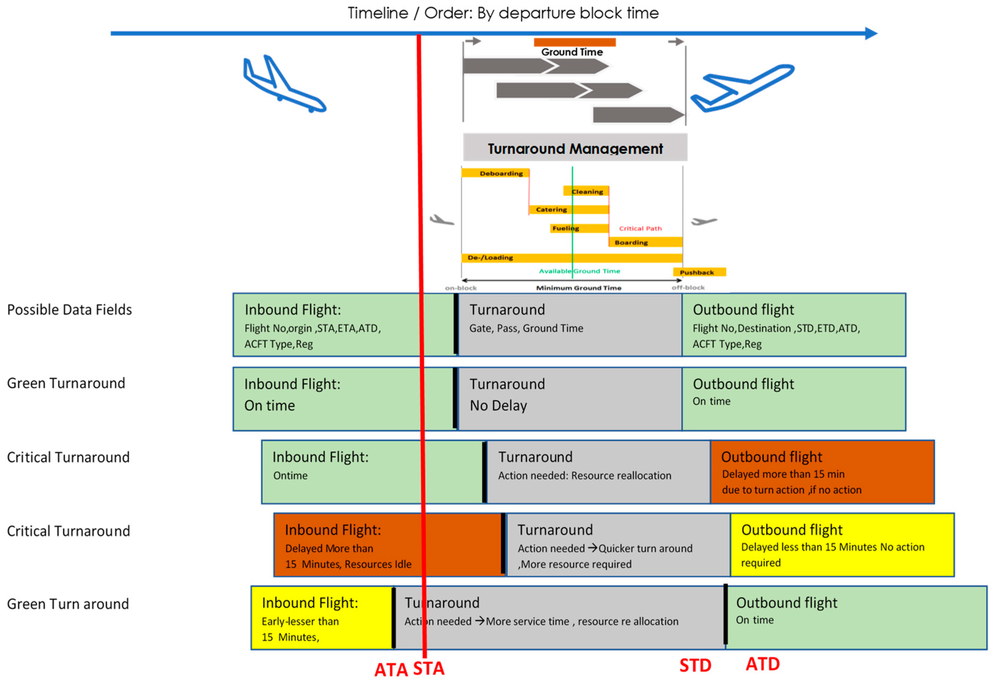
A turnaround management system should be able to determine the target and actual times for every ground handling (sub-)process. The most significant and challenging aspect of establishing a competent turnaround management system is gathering essential data on activities performed by service providers (or internal airline departments) during ground handling. Figure 1 shows the overall Gantt chart schematic for turnaround time and the impact of flight time variation. If the actual time of arrival (ATA) is within a tolerance value (decided by the operator/regulator) of +/−15 min of the scheduled time of arrival (STA), we consider it on time and the corresponding departure actual time of departure (ATD) is within a tolerance limit of +/−15 min of the scheduled departure time, we can consider it on time and it is indicated in green turnaround (green colour in Figure 1). When flight arrival is delayed, there is a potential that the entire turnaround procedure will be delayed, which we refer to as the critical turnaround process. If the inbound aircraft is delayed and the scheduled padding time (the extra buffer time between arrival and departure) is insufficient, the outbound flight will be delayed. Figure 1 highlights how ground resource management affects various procedures involved in the turnaround (such as de-boarding, cleaning, catering, fueling, and boarding) and how delays in these processes might cause further delays in departure.

Machine learning models, such as multiple linear regression (MLR) and multilayer perceptron (MLP), are increasingly used to predict flight arrival and departure times and improve the efficiency of resource allocation during the turnaround process. The MLR-based model is commonly used to predict arrival time based on the departure time from the same airport, leveraging historical data. MLP, on the other hand, can capture more complex relationships between variables but requires more data and computational resources. Several studies have explored the use of these models for predicting flight arrival and departure times, including Koo and Cheong’s analysis of airline on-time performance [29] and Aoki et al.’s study on predicting flight arrival times with machine learning methods [30]. Effective feature engineering is crucial to the success of machine learning models such as multiple linear regression (MLR) and multilayer perceptron (MLP) in predicting flight arrival and departure times [29]. By carefully selecting and engineering relevant features, these models can capture important patterns and relationships in the data, leading to more accurate predictions. We will discuss the process of feature engineering in more detail in the next session. We used the MLR regression model to predict arrival time based on departure time from the same airport (for example, based on the flight’s departure time from Dubai Airport, the same flight’s return arrival time at Dubai Airport would be predicted based on historical data).

2.2. Exploratory Data Analysis

The data used is on the scheduled and actual movement of flights operated to and from Dubai Airport from October 2021 to October 2022. According to Airport Council International records, Dubai International Airport is ranked first in terms of overall international passenger handling (29,110, 609—international passengers enplaned and deplaned) during the year 2021 [31], and the airport handles a wide range of aircraft types. We chose Dubai International Airport data for our research because it has growing passenger and aircraft movement and, thus, in the near future resource planning will be a key concern for ground handling.

The data was extracted from Flightradar24 [32]. We first compared scheduled hourly flight movement to actual flight movement. For this analysis, we used the scheduled and actual flight arrival and departure times for every hour of the day. Based on the data collected, we performed a comprehensive numerical and graphical comparative analysis of variation in actual and scheduled flights for Dubai International Airport on various days. 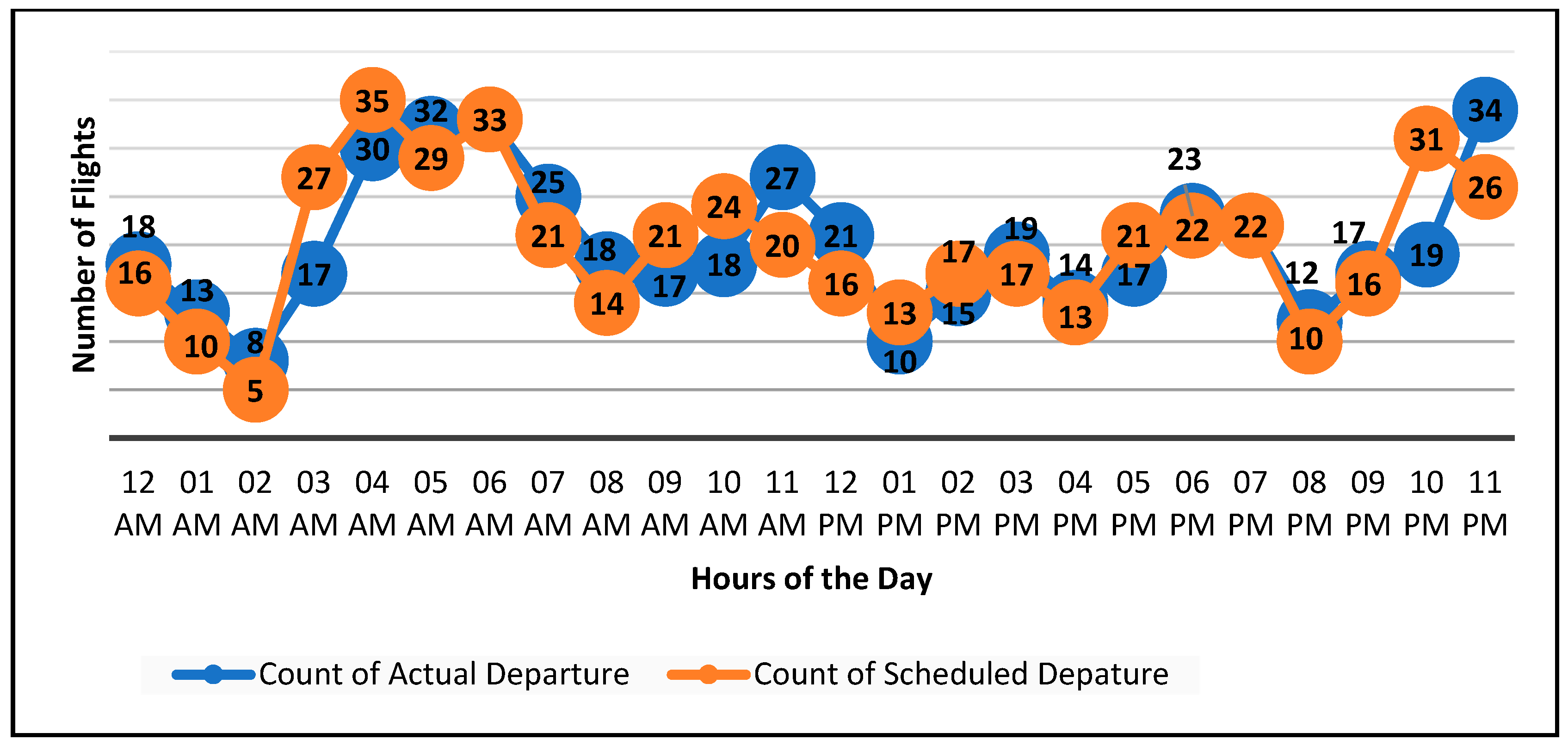Figure 2 shows a detailed comparison of hourly departure flights planned as per schedule with actual departures from Dubai International Airport for each day. Figure 2 shows that the number of flights handled every hour varies significantly between scheduled and actual movement. This will result in variations in ground resource requirements during the day, as certain ground resource requirements will remain so until the flight departs. This will have an impact on arrivals for which ground resources are assigned, and it may also introduce delays in service for the arrival of subsequent departures if the ground handling resource planner is unable to foresee such requirements. 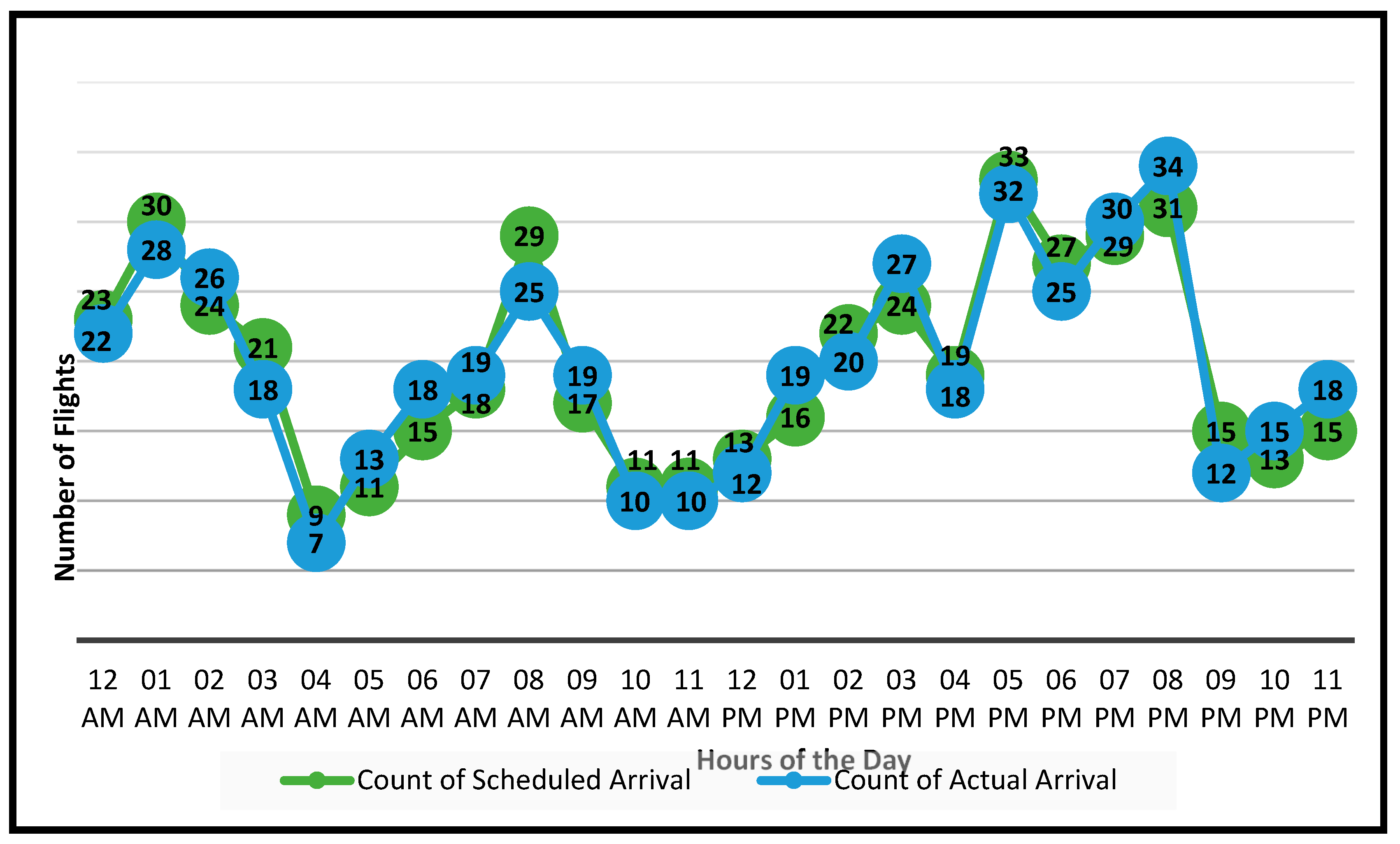A similar comparison was made for arrival flights in Figure 3.

Figure 3 shows that the actual number of arrivals differs considerably from the schedule most of the time. Typically, ground handling workforce allocation planning for future flights on the same day is done well in advance based on schedules (8–10 h in advance based on shift timings with duty roster) [33]. Most airports have arrival flights followed by departure flights, termed a bank, which results in large peaks in airport resource demand [34]. To generate demand curves, evaluations mainly use resources for flight schedules, which are frequently insufficient in real-time. In certain cases, tasks may be linked to flight locations. The flight position is important in defining the resources available; there are different types, such as a hard stand or a tube stand. Flight delay or early arrival usually results in a different stand allocation and resource planning.

Figure 4 illustrates a comprehensive view of scheduled and actual flights arriving between 00:00–08:00 h. The graph in Figure 4 shows that the number of scheduled flight arrivals and actual flight arrivals vary substantially depending on the hour of the day. Consider the first hour (01:00–01:59 h), when 30 arriving aircraft were scheduled for the hour and 21 flights landed in the same hour. The remaining 6 flights landed between 00:00–00:59 h, with 2 flights landing between 02:00 and 02:59 h and 1 flight landing between 23:00–23:59 h. Such flight delays (both early and late from the scheduled time) could potentially result in significant variations in ground resource mobilisation and simultaneous ground resource requirements at different hours of the day. It can also be inferred from Figure 4 that the shift in the number of aircraft resulted in a variation of the fleet combination scheduled for the hour and this will result in fluctuations in ground resource requirements.

We then analysed aircraft-specific arrival time variation to assess the impact of actual and scheduled flight time variation. We classified the difference between actual flight arrival and scheduled flight arrival time. If the difference between the actual and scheduled arrival time is more than 15 min, it is classified as ‘Delay’; if the difference between the actual and scheduled landing time is less than −15 min, it is classified as ‘Early’; and if the flight arrives within +/−15 min of the scheduled time, it is classified as ‘On Time’. Initially, we examined the most frequent type of aircraft operating at Dubai Airport for 3 days and computed total schedule temporal variations (On time, Early, and Delay) using the above classification criteria. We then analysed aircraft-specific arrival time variation to assess the impact of actual and scheduled flight time variation.

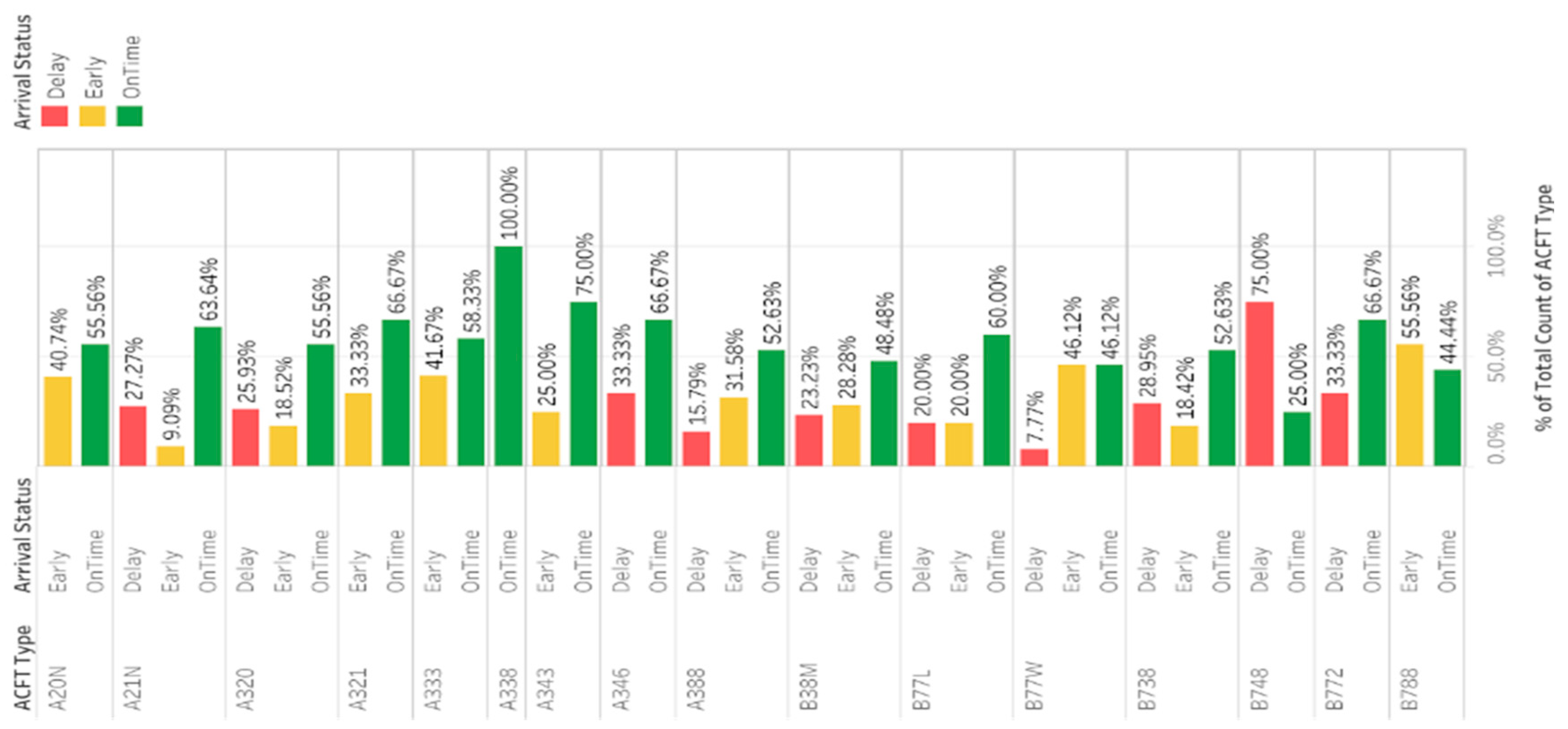
The distribution in Figure 5 shows that more than 70% of flights are either ‘Early’ or ‘On Time’ in most aircraft types. However, because the departure schedule time is dependent on the departure schedule/slot, the aircraft may occupy the bay for an extended period and various ground resources teams (ladder, boarding, a.m.Es, auxiliary power unit) may provide additional service time to specific aircraft. This will also affect the operational efficiency and productivity of ground handling resources (both human and equipment) in most aircraft types.

One of the consequences of delayed arrivals and departures is the allocation of aircraft stands in remote locations. If the ground resource planner distributes resources to an adjacent bay and the delayed arrival apron management allocates a stand at a remote location, service delay will be imposed—the issue being that the movement of resources to their (remote) point of use adds waste to the process. All these factors have an impact on operational efficiency and the underutilisation of airport resources, which requires machine learning approaches to predict arrival time and improve stand and resource allocation. In this study, we also examine the utility of a linear regression model in predicting the exact landing/arrival time for each flight based on flight departure time from the same airport. This will allow the ground resource management team to assign resources to the same aircraft based on its departure time and utilise optimal ground resource requirements for specific hours, as well as establish a future efficient stand allotment strategy.

Finally, we comprehensively examined the influence of arrival time variation on departure time variation.

Table 1. Comparative analysis of arrival time variation and its impact on corresponding departure of Dubai International Airport.

Arrival	Early			OnTime			Delay
Departure	Delay	Early	On Time	Delay	Early	On Time	Delay	Early	On Time
Hours
12 a.m.	11%	0%	89%	24%	0%	76%	78%	0%	22%
01 a.m.	16%	0%	84%	27%	1%	72%	87%	1%	12%
02 a.m.	14%	4%	82%	26%	1%	72%	70%	0%	30%
03 a.m.	13%	0%	87%	17%	0%	83%	63%	0%	37%
04 a.m.	6%	3%	91%	16%	1%	83%	60%	0%	40%
05 a.m.	33%	0%	67%	26%	0%	74%	78%	0%	22%
06 a.m.	13%	0%	87%	21%	0%	79%	65%	0%	35%
07 a.m.	10%	0%	90%	16%	0%	84%	72%	0%	28%
08 a.m.	20%	0%	80%	27%	0%	73%	88%	0%	12%
09 a.m.	9%	3%	88%	16%	1%	83%	70%	0%	30%
10 a.m.	9%	0%	90%	20%	0%	80%	63%	0%	37%
11 a.m.	8%	2%	91%	25%	1%	74%	80%	0%	20%
12 p.m.	8%	1%	91%	20%	0%	80%	69%	0%	31%
01 p.m.	11%	1%	88%	21%	0%	79%	84%	0%	16%
02 p.m.	18%	0%	82%	22%	0%	78%	79%	0%	21%
03 p.m.	15%	0%	85%	23%	1%	76%	82%	0%	18%
04 p.m.	6%	1%	93%	19%	0%	80%	81%	0%	19%
05 p.m.	10%	1%	89%	35%	0%	65%	88%	0%	12%
06 p.m.	-%	1%	93%	19%	0%	80%	84%	0%	16%
07 p.m.	10%	0%	90%	17%	0%	83%	55%	0%	45%
08 p.m.	10%	1%	89%	20%	0%	80%	71%	0%	29%
09 p.m.	18%	0%	82%	25%	0%	75%	68%	0%	32%
10 p.m.	14%	0%	85%	28%	1%	72%	91%	0%	9%
11 p.m.	0%	0%	100%	75%	0%	25%	100%	0%	0%
Day	11%	1%	88%	22%	0%	78%	74%	0%	26%

illustrates the number of hourly percentage arrival time variation categories in relation to the corresponding departure category during the day. The same aircraft was scheduled to depart from Dubai Airport during the day, both on time and late. The results indicate that 74% of delayed arrivals (aircraft with the same registration depart within 3 hours of their scheduled arrival time) from Dubai Airport during the study period. Similarly, 11% of the early-arrived flights were delayed. However, 26% of delayed planes were able to recoup their time in Dubai. The arrival time variation fluctuates throughout the day, indicating the corresponding departure time. The overall variation indicates the importance of arrival time in the turnaround process. The aggregate variation arrival and departure variations are shown in the last row of Table 1.

Exploratory data analysis provided a greater insight into the various factors affecting ground resource allocation at airports. It has been found that the number of flights, the type of aircraft variation, arrival delays, and departure delays all have an impact on resource allocation. In addition, predicting the arrival time of round-trip flights based on the departure time from the same airport can be highly beneficial for efficient resource allocation. This is because more than 50% of the arrival traffic at the airport is actually departing from the same airport.

By accurately predicting the arrival time of round-trip flights, airport ground staff can proactively allocate resources, such as gates, baggage carousels, and ground handling equipment, to the flights. This reduces wait times for passengers and improves their overall experience. Furthermore, it can help airport operators optimise the use of their resources, reducing waste and improving profitability.

Moreover, knowing the distribution of hourly arrivals and the type of aircraft that are scheduled to arrive can also help in allocating resources efficiently. For example, if there is a higher number of heavy or wide-body aircraft like the B777 and A380 scheduled to arrive, the airport ground staff can allocate more ground handling equipment and personnel to accommodate these flights. Similarly, if there are more narrow-body aircraft arriving during off-peak hours, the airport can allocate fewer resources to these flights and optimise the use of resources elsewhere.

2.3. The Feature Engineering

Exploratory data analysis, as described in Section 2.2, played a crucial role in identifying key features in the dataset. For our model development, we initially used 40 features, including derived features such as departure and arrival information for the first and second departure stations, scheduled and actual flying times, departure delays, and departure delay categories (On Time/Early/Delay). Additionally, we created a derived feature, the exponential moving average (EMA) of the previous flying times based on the previous flight (same aircraft type) on the same origin–destination (OD), to capture the temporal variation of flying time [7].

Based on domain expertise and descriptive analytics, we identified critical features with an impact on arrival delay. To perform feature engineering, we used the backward elimination approach, where categorical variables were converted to numerical variables using the one-hot encoding technique. First, a multiple linear regression model was fit with the most relevant features based on domain expertise. Then, the feature with the highest p-value (i.e., the least significant) was removed from the model, and the model was refit. This process was repeated until all remaining features had a significant p-value.

The study focuses on predicting the arrival delay time and its classification (multiclass: Early, On Time, Delay). For both classification and regression problems, the same set of features identified through the feature engineering process were used.

Table 2. Features selected for model development.

SN.	Feature	Description
1	WEEK_DAY	weekday in which the flight was performed
2	Aircraft ID_2	schedule ID from Origin 2
3	Origin 2	airport of second departure
4	Destination 2:	airport of arrival
5	SFT	scheduled flying time
6	ATD_1: Actual DEP	actual departure time
7	DEP_DEL_CAT_1	departure delay category of Origin 1
8	DEP_DEL_1	departure delay in minutes of Origin 1
9	STA_2	scheduled arrival time at same departure airport
10	AICRAFT_2	type of aircraft
11	EMA_FT	exponential moving average of flying time
12	ARR delay	arrival delay in minutes (one of our dependent variables)
13	ARV_DEL_CAT	classification arrival delay (one of our dependent variables)

lists the dependent and independent variables used for machine learning model development (training and testing), which included basic and derived features. Among these variables, the arrival delay in minutes (ARR delay) and its classification (ARV_DEL_CAT) were considered dependent variables while the remaining features were treated as independent variables.

2.4. Multiple Linear Regression (MLR)

Linear regression is a modelling technique for analysing data to make predictions [35]. We consider the landing time prediction problem as a regression problem. The linear regression model fits a linear equation from observed data between the dependent variable (Y) and input independent variables (X), including derived features that capture relevant information from the data. Linear models are characterized by linear predictor functions, which estimate unknown model parameters from the data. These models enable the estimate, E[Y], to depend on multiple independent variables and to exhibit shapes other than straight lines, although they do not allow for arbitrary shapes. The significance of incorporating derived features in a multiple linear regression model lies in the improved accuracy and interpretability of the model, as these features help capture complex relationships and patterns in the data, leading to more accurate predictions. Adding this feature helps capture complex relationships and patterns in the data, particularly the influence of historical flight duration trends on the current landing time. This information allows the model to account for any gradual changes or fluctuations in flying time, leading to more accurate predictions and a better understanding of the underlying factors affecting landing time.

The MLR model for predicting arrival delay ($AR{R}_{Delay})$ using features in Table 2 is as follows:

$$\begin{gathered} AR{R}_{Delay}={\beta }_0+{\beta }_{1}WEE{K}_{DAY}+{\beta }_{2}Flight I{D}_2+{\beta }_{3}Origin 2+{\beta }_{4}Destination 2 \\ \hspace{1em}\hspace{1em}\hspace{1em}\hspace{1em}\hspace{1em} \hspace{1em}\hspace{1em}\hspace{1em}+{\beta }_{5}SFT+{\beta }_{6}ATD\_1+{\beta }_{7}DEP\_DEL\_CAT\_1+{\beta }_{8}DEP\_DEL\_1 \\ \hspace{1em}\hspace{1em} +{\beta }_{9}STA\_2+{\beta }_{10}AIR\_CRAFT\_2+{\beta }_{11}EMA\_FT+\epsilon \end{gathered}$$

(1)

where:

ARR_Delay is the dependent variable or the output variable that we are trying to predict or explain, which represents the arrival delay in minutes for a flight.

β₀ is the intercept or constant term of the model, which represents the expected value of ARR_Delay when all the independent variables are zero. β₁–β₁₁ are the regression coefficients for the respective independent variables, which indicate the strength and direction of the relationship between each variable and the ARR_Delay.

WEEK_DAY is a categorical variable representing the day of the week, which is typically encoded as a set of binary variables (e.g., 0/1 for Monday/Tuesday). Flight ID₂, Origin 2, and Destination 2 are categorical variables representing the flight ID, origin airport, and destination airport, respectively, which are typically encoded using dummy variables. SFT, ATD_1, DEP_DEL_CAT_1, DEP_DEL_1, STA_2, AIR_CRAFT_2, and EMA_FT are continuous variables representing the scheduled flight time, actual time of departure from origin airport 1, departure delay category, departure delay, scheduled time of arrival, aircraft type, and estimated maximum altitude, respectively. ε is the error term or residual, which represents the variability or uncertainty in the model that is not explained by the independent variables.

The goal of the multiple linear regression model is to estimate the values of the regression coefficients that minimise the sum of the squared errors between the predicted and actual values of ARR_Delay. This enables us to identify the most important independent variables that are associated with ARR_Delay and make predictions of ARR_Delay for new flights based on the values of the independent variables.

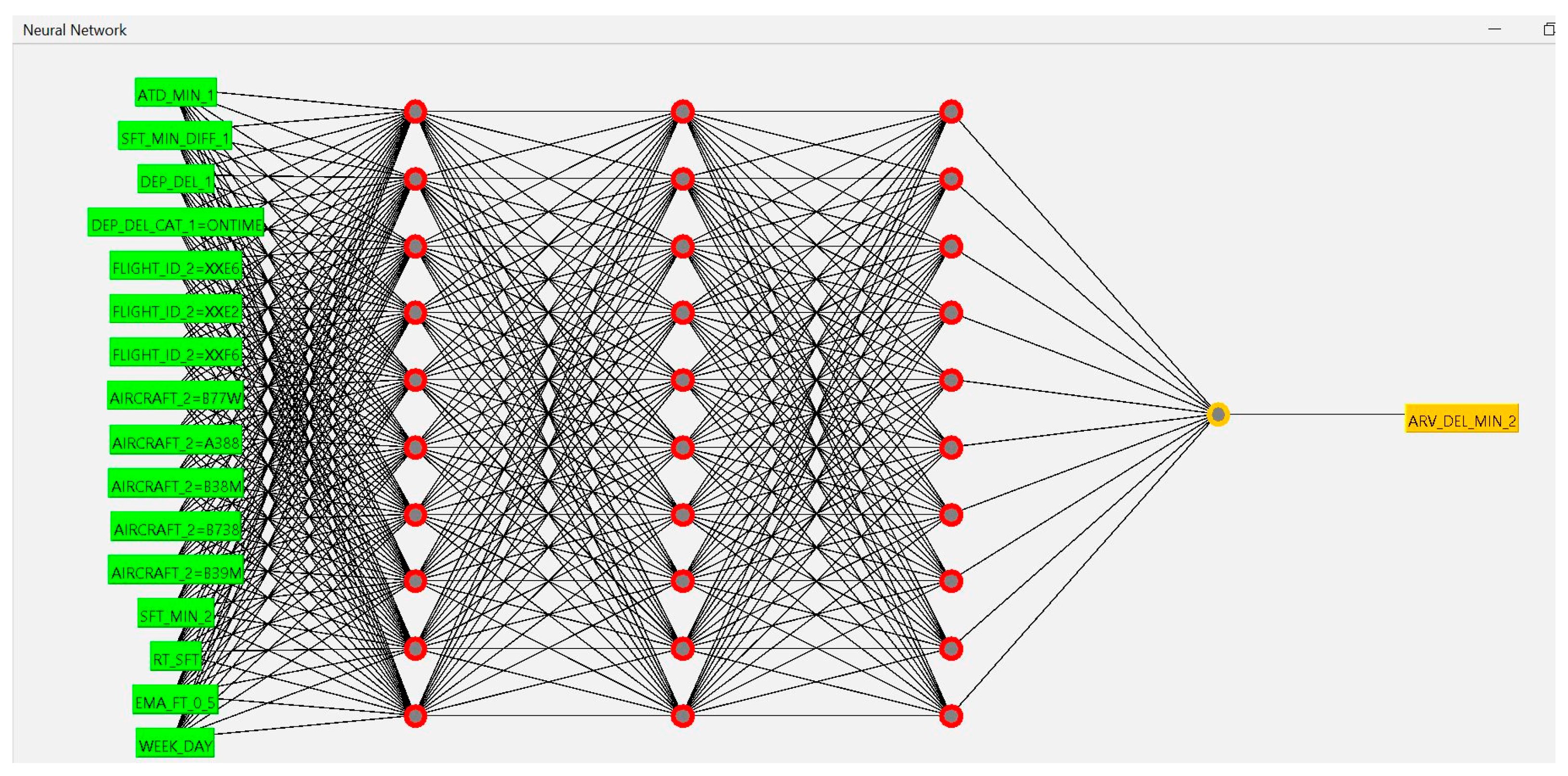
2.5. Multilayer Perceptron (MLP)

Artificial neural networks (ANN) have recently been widely used in different sectors, such as medical applications, pharmaceutical sciences, engineering, finance, social media, and other areas [36]. One of its most significant benefits is its capacity to quickly learn from its surroundings (e.g., data and tasks). During training, it can also detect redundant and noisy variables [36]. Because of its reliability and superior performance, we selected the multilayer perceptron (MLP) to predict scheduled flight arrival times using ANN. Most machine learning algorithms generate excellent results only when their parameters are calibrated and modified appropriately [37]. MLP is a type of neural network that consists of an input layer, one or more hidden layers, and an output layer. In the case of multiclass classification, the MLP is designed to predict the class of a given input by assigning it to one of several possible categories.

Input Layer:

The input layer takes the input features $X=(x_1,x_2,...,x_n)$ and applies no activation function. Therefore, the output of the input layer is the same as the input features, which can be written as:

$$H^0=X$$

(2)

Hidden Layers:

Each hidden layer in the MLP applies an activation function g to the linear combination of the input features or the outputs of the previous layer. The output of the l^th hidden layer, denoted as $H^l=h^{l_1},h^{l_2}\dots ,h^{l_{N-1}}$, can be obtained using the following equation:

$$H^l=g\left(W^l{H}^{l-1}\right)+b^l$$

(3)

where $W^l$ is the weight matrix of the l-th layer, $b^l$ is the bias vector of the l^th layer, and g is the activation function applied element-wise to the linear combination of the input features or the outputs of the previous layer.

Output Layer:

The output layer applies a specific activation function f depending on the problem type, such as softmax for multiclass classification, sigmoid for binary classification, or linear for regression. The output of the MLP, denoted as Y, is computed as follows:

$$Y=f\left(W^L{H}^{L-1}\right)+b^L$$

(4)

where $W^L$ is the weight matrix of the output layer, $b^L$ is the bias vector of the output layer, and $H^{L-1}$ is the output of the last hidden layer.

Note that in this notation, superscript l refers to the layer number, and the notation superscript $l_j$ refers to the j^th unit in the l^th layer.

In the case of multiclass classification, the softmax function is commonly used to ensure that the output probabilities sum to 1. The output of the MLP can be represented as a vector $Y=y_1,y_2,..y_k$ where k is the number of classes and $y_i$ represents the probability of the input data belonging to the i-th class.

For model training and testing, we utilised the specified 75–25 split with k-fold cross-validation; in our case, k was equal to ten (k =10). Following various trails experiments with our dataset, the following hyperparameters were chosen: (a) hidden layer sizes: (10, 10, 10); (b) epoch: 500; (c) learning rate: 0.3; (d) solvers: stochastic gradient descent (Sgd) and Adam; and (e) L2 penalty (regularisation term) parameters: 0.001 and 0.05, 10.

In this study, we propose MLP models to predict both arrival time and arrival delay classification (Early, On Time, and Delay). Since the output variable is categorical, the MLR model was not chosen for this classification. The MLP was trained using input features corresponding to serial numbers 1–11 in Table 2, and the output variable was the predicted arrival delay in minutes (SN-12 in Table 2). Additionally, we used the features listed in Table 2, corresponding to serial numbers 1–11, to classify the round-trip arrival categories based on departure time. The output variable for this classification task was ARV_DEL_CAT (SN-13 in Table 2).

The performance of supervised learning models for predicting landing time was evaluated using mean absolute error (MAE) and root mean squared error (RMSE), R-squared (R2), T-statistics, and p-values where

MAE: This metric measures the average absolute difference between the predicted values ($\widehat{y}$) and the true values (y) over a set of n instances.

$$MAE=\frac{1}{n}\sum _{k=1}^n|y_k-{\widehat{y}}_k|$$

(5)

A smaller value of MAE means better performance, as the model predictions will be closer to true values on average.

RMSE: This metric measures the square root of the average squared difference between the predicted values and the true values over a set of n instances.

$$RMSE=\sqrt{\frac{1}{n}\sum _{k=1}^n(y_k-{\widehat{y}}_k)\text{^}2}$$

(6)

Like MAE, a smaller value of RMSE also means better model performance. However, RMSE places more emphasis on large errors, as it involves taking the square root of the sum of squared errors, which gives higher weight to larger errors.

R-squared (R2): This measures the proportion of variation in the dependent variable that is explained by the independent variables in the model. It ranges from 0 to 1, with higher values indicating a better fit.

T-statistics: These are used to test the significance of each independent variable in the model. A t-value greater than 2 or less than −2 typically indicates statistical significance at the 95% confidence level.

p-values: These are used to test the null hypothesis that the coefficient for each independent variable is zero. A p-value less than 0.05 (or whatever alpha level is chosen) indicates statistical significance at the chosen level.

Accuracy: The performance of the classification of the MLP model was evaluated by accuracy. One commonly used metric is the “accuracy score”, which is the ratio of the number of correctly classified instances to the total number of instances in the dataset.

Accuracy = (True Positive + True Negative)/Total Number of Sample

(7)

3. Results

3.1. Scenario 1 (One Origin–One Destination—1 Round-trip)

The analysis was carried out to predict different segments of multileg flights. Initially, we analysed the prediction capability of the proposed method in predicting the landing time of two legs using departure time variation, aircraft type, hours of operation, destination, aircraft registration, the exponential moving average of flying of previous flights, and scheduled flying time for both outbound and inbound. Holt [38] introduced exponentially weighted moving averages (EMA) for seasonal and trend forecasting. The EMA’s reaction is directly dependent on the data pattern. The EMA offers more weight to recent values of flying time, and as a result, it could be a superior model for capturing trends over time in a faster manner [7]. The data was split into training (80%) and test set (20%). The MLR model was developed through 10-fold cross-validation.

The model predicted the arrival time with an RMSE of 8.01 min and an MAE of 7.56 min. This means that, under normal operating conditions, based on the departure time from Dubai Airport, the same flight’s arrival time (return from the destination airport) to Dubai Airport can be predicted with an accuracy of 8 min. A sample of prediction results using test data for a scheduled flight operated between Dubai International Airport (DXB) and Jakarta International Airport (CGK), and return to Dubai International Airport on different days, as shown in Table 1. The last column (Predicted _ATA) in

Table 3. Sample prediction results with relevant fields for scheduled aircraft arrival time predicted by proposed model (Predicted ATA_2) and actual arrival time (ATA_2) at Dubai airport on various days.

ID	DATE	Orgin	Dest	Aircraft	Flight Time	STD	ATD	Dep Delay_1	ID_2	Dest_2	Flight Time_2	STA_2	ATA_2	Predicted ATA_2
XX	25/09/2022	DXB	CGK	B77W	08:02:00	00:10:00	00:37:00	27	XY	DXB	07:15:00	18:55:00	18:19:00	18:30:00
XX	24/09/2022	DXB	CGK	B77W	08:04:00	00:10:00	00:26:00	16	XY	DXB	07:11:00	18:55:00	18:29:00	18:24:00
XX	23/09/2022	DXB	CGK	B77W	07:58:00	00:10:00	00:26:00	16	XY	DXB	07:13:00	18:55:00	18:14:00	18:15:00
XX	22/09/2022	DXB	CGK	B77W	08:02:00	00:10:00	00:39:00	29	XY	DXB	07:12:00	18:55:00	18:13:00	18:18:00
XX	21/09/2022	DXB	CGK	B77W	08:06:00	00:10:00	00:22:00	12	XY	DXB	07:11:00	18:55:00	18:17:00	18:21:00
XX	20/09/2022	DXB	CGK	B77W	07:54:00	00:10:00	00:24:00	14	XY	DXB	07:18:00	18:55:00	18:28:00	18:27:00
XX	19/09/2022	DXB	CGK	B77W	07:49:00	00:10:00	00:21:00	11	XY	DXB	07:22:00	18:55:00	18:22:00	18:30:00
XX	18/09/2022	DXB	CGK	B77W	07:55:00	00:10:00	00:28:00	18	XY	DXB	07:21:00	18:55:00	18:24:00	18:20:00

represents the arrival time predicted by the proposed model, whereas ATA_2 provides the actual arrival time and STA_2 represents the scheduled arrival time. A similar analysis was carried out for flights from Dubai (DXB) to Paris (CDG) and returning to Dubai, and the ETA was estimated with an RMSE of 10.2 min.

Our findings showed that, in using feature engineering, the MLR model was able to predict the arrival time with 10 min of variation before 14 h (hours) to 16 h (for example, in Table 3, the destination airport is located at around 7 h of flying time) of the actual arrival time of the scheduled flight. The MLR model was able to predict the variation in arrival time based on historical travel time and its temporal variations. This will enable the ground resources management team to optimally deploy resources and determine hourly traffic density well in advance.

Based on data analysis, we observed that, on average, 50% of scheduled flights originating from Dubai (Emirates and Fly Dubai airlines are the top 2 airlines operated from Dubai airport to multiple destination round-trip flights) to other airports return to Dubai after a normal turnaround time since it is a hub airport, making the prediction of next arrival time from the departure time of the same airport practically achievable. Most of these round-trip flights return to Dubai within 3 h to 16 h (depending on the length of the short and long-haul flights) of their scheduled departure time.

3.2. Scenario 2 (One Origin–Multiple Destination—Multiple Round-trip)

The analysis was performed to predict several scheduled flights with different destination airports. In the previous section, we examined the MLR method’s suitability to estimate the landing time of the two legs. In comparison to the preceding Scenario 1 input attributes, the Origin and Aircraft ID were regarded as new features for the MLP model due to the involvement of several flights with various destinations in this model. In this scenario, we used MLR and a multilayer perception model to estimate arrival time delays and classify arriving flights based on whether they would arrive early, late, or on time. In order to assess the model’s suitability and robustness, we compared the prediction results of scheduled flights from Dubai to three international airports: Venice, Madrid, and Karachi (IATA: VCE, MAD, and KHI) by different airlines and aircraft types (B77W, A388, and B738). This includes different flight lengths and different types of carriers and different flight types with their 1-year operations. The performance of both conventional and selected processes was measured using the classic evaluation metric coefficient of determination R2, which is the measure of deviation between the regression line and the observed points.

In statistical hypothesis testing, p-values represent the probability of obtaining results as extreme as the observed results, assuming that the null hypothesis is true. A p-value less than the significance level (typically 0.05) indicates that the observed results are unlikely to have occurred by chance alone, and therefore, the null hypothesis can be rejected. In the table above, the p-values and t-values correspond to each variable included in the regression model. The t-values represent the number of standard deviations that the estimate is from the null hypothesis. A positive t-value means that the estimate is higher than the null hypothesis, while a negative t-value means that the estimate is lower than the null hypothesis. The results in

Table 4. The p-values and t-values correspond to each variable included in the regression model.

Variable	t-Value	p-Value
ATD_MIN_1	3.608071	3.41 × 10−4
SFT_MIN_DIFF_1	−0.05753	9.54 × 10−1
DEP_DEL_1	5.810073	1.14 × 10−8
SFT_MIN_2	−2.858086	4.45 × 10−3
RT_SFT	−2.252719	2.47 × 10−2
EMA_FT_0_5	−2.231050	9.82 × 10−2
WEEK_DAY	0.683288	4.95 × 10−1
AIRCRAFT_1_A388	−2.050793	4.08 × 10−2
AIRCRAFT_1_B38M	−3.999751	7.35 × 10−5
AIRCRAFT_1_B39M	−3.984051	7.83 × 10−5
AIRCRAFT_1_B738	−3.995765	7.47 × 10−5
AIRCRAFT_1_B77W	−2.114035	3.50 × 10−2
AIRCRAFT_2_A388	−2.050793	4.08 × 10−2
AIRCRAFT_2_B38M	−3.999751	7.35 × 10−5
AIRCRAFT_2_B39M	−3.984051	7.83 × 10−5
AIRCRAFT_2_B738	−3.995765	7.47 × 10−5
AIRCRAFT_2_B77W	−2.114035	3.50 × 10−2
DEP_DEL_CAT_1_DELAY	−2.953275	3.30 × 10−3
DEP_DEL_CAT_1_ONTIME	−2.906892	3.82 × 10−3
FLIGHT_ID_2_XXE2	−1.416237	1.57 × 10−1
FLIGHT_ID_2_XXE6	−2.93281	3.52 × 10−3
FLIGHT_ID_2_XXF6	−4.036457	6.32 × 10−5

indicate that a significant number of variables exhibit p-values below 0.05, suggesting their statistical significance and leading to the rejection of the null hypothesis for these variables. These variables include DEP_DEL_1, EMA_FT_0_5, AIRCRAFT_1_B38M, AIRCRAFT_1_B39M, AIRCRAFT_1_B738, AIRCRAFT_2_B38M, AIRCRAFT_2_B39M, AIRCRAFT_2_B738, FLIGHT_ID_2_XXE6, FLIGHT_ID_2_XXF6, DEP_DEL_CAT_1_DELAY, and DEP_DEL_CAT_1_ONTIME. For the t-values (Table 4), we can see that variables with absolute t-values greater than 2 can be considered statistically significant. Therefore, DEP_DEL_1, EMA_FT_0_5, DEP_DEL_CAT_1_DELAY, DEP_DEL_CAT_1_ONTIME, AIRCRAFT_1_B38M, AIRCRAFT_1_B39M, AIRCRAFT_1_B738, AIRCRAFT_2_B38M, AIRCRAFT_2_B39M, AIRCRAFT_2_B738, FLIGHT_ID_2_XXE6, and FLIGHT_ID_2_XXF6 can be considered statistically significant.

The MLR model prediction performance for the features selected was evaluated using residual analysis. The residual ($\epsilon$) is calculated using

$$\epsilon =y-\widehat{y}$$

(8)

where y is the actual (observed) value and $\widehat{y}$ is the predicted value.

The heteroscedasticity plot in Figure 6a indicates the residuals have a constant variance across the predicted value. The residuals are centred around zero and have a symmetrical distribution, with most of the residuals being close to zero. This is a good indication that the model has a good fit for the data and the residuals are randomly distributed around zero. However, the low density of points away from the origin may indicate the presence of some outliers or influential data points that are having a significant impact on the model. It is important to investigate these points further to ensure they are not skewing the model results. The MLR model has a good fit to the data, as the residuals are randomly distributed around zero and the Q-Q plot shows that the residuals follow a normal distribution. The fact that most of the residuals are within 2 times the standard deviation line also indicates that the model is doing a good job of predicting the response variable. The Q-Q plot in Figure 6b is a graphical method for assessing whether the residuals follow a normal distribution. Some of the points in the Q-Q plot deviate from the 45-degree (red) line, which suggests that the residuals are not perfectly normally distributed. Specifically, the points at the ends of the Q-Q plot are deviating from the red line, which indicates that the tails of the distribution are not perfectly normal.

The departure from normality observed in the model could be attributed to a number of factors, including the existence of outliers or the presence of a nonlinear relationship between the predictors and the response variable. To address these potential issues, it is important to further investigate and evaluate the model using alternative techniques to ensure that it is still performing well despite the deviations from normality. In this regard, an MLP model with 3 hidden layers was developed to predict arrival delays, as depicted in Figure 7. The MLP model can be used to identify nonlinearity or outliers that may be present in the data and help improve the overall performance of the model.

The MLP model has three hidden layers, each containing 10 neurons. The activation function used is the rectified linear unit (ReLU). The solver used is the adaptive moment estimation (Adam) algorithm, which is an optimisation algorithm that is well-suited for large datasets. The model is trained for a maximum of 500 iterations (epochs), and the random state is set to 2 to ensure the reproducibility of the results. The evaluation of the model shows a moderate correlation coefficient of 0.6406, which indicates a good linear relationship between the predicted and actual target values. The mean absolute error and root mean squared error are 9.2085 and 11.188, respectively, which indicates that the model’s predictions have a moderate degree of error.

3.3. Classification of Arrival Category

Here, we configured a MLP classification model for predicting the arrival delay category (ARV_DEL_CAT) based on the departure delay category and other input parameters from the first origin. The MLP model was configured with the same inputs as the MLP regression model and the output variable was classified into three categories: Early, On Time, and Delay. The proposed MLP classification model is illustrated in Figure 8, which consists of one input layer, three hidden layers, and one output layer with three classes as the output. The model was able to classify the arriving category (Early/On Time/Delay) of round-trip flights at Dubai International Airport, using input parameters of departing time, departure delay category, and other relevant factors.

Since most delay prediction studies [14,30,39,40] considered arrival time based on previous departure time (same leg), our study predicts arrival time based on departure time before the two flight legs’ departure time, and there are no prior benchmarks available for prediction performance comparison. However, we evaluated the proposed model’s performance metrics using MLR and MLP, as shown in

Table 5. Performance comparison of arrival delay time prediction.

	MLR	MLP
Correlation coefficient (R2)	0.698	0.6406
MAE	7.7423	9.2085
RMSE	10.0768	11.188

. The findings show that the MLR model performs slightly better than the multilayer perceptron with 11 input attributes for round-trip aircraft arrival delay prediction, and the MLR model was able to capture fluctuations using a linear combination of elements. Because there are no benchmarks available to compare our model to multileg arrival time prediction, we compared our prediction result to a single leg with a shorter forecast horizon.

In the given Table 5, the MLR model has a lower MAE and RMSE than the MLP model, indicating that the MLR model provides better accuracy in predicting the dependent variable. Further analysis was carried out to determine the reason for the MLR model’s better performance. It was found that the MLR model was able to provide good prediction accuracy for small variations, but struggled with large nonlinear variations. The MLP model was not able to capture these nonlinearities. The data had some nonlinearity/outliers that could not be modelled by the selected parameters in the available features of the dataset. The domain knowledge suggested that these variations were due to random variations in flying time caused by speed variation, weather, traffic density, and deviations, which were not available in the present dataset. However, considering the prediction horizon and the intended usage of the model for resource allocation, the accuracy of the model was significantly good for resource planning.

In

Table 6. Performance comparison of arrival delay classification prediction with previous studies.

Study	Model	Number of Features	Number of Flight Legs Ahead	Accuracy (%)
Thiagarajan et al. [40]	Gradient Boosting with Binary Classification (Delay/No Delay)	16	1	94.3
Qu et al. [39]	SE-DenseNet with Multiclass	81	1	93.19
Proposed Model	MLP with Multiclass (Early, On Time, and Delay)	11	2	93.57

, we compare the accuracy of our model to that of previous studies [30,32] that classified arrival time based on previous departure time. Previous studies were mostly focused on single-leg flight operations from origin to destination; however, the proposed study focuses on round-trip arrival time prediction for that prediction horizon with greater than double the duration of the single-leg flight. Our model for Dubai International Airport with training and testing had a score of 93.57% and is comparable to [40], which achieved a mean accurate prediction of 94.3%. The prediction time horizon of the two models can be analysed as follows: The first model predicts the arrival time at Dubai airport from the origin airport with a lead time of 5 h. On the other hand, the proposed model predicts the arrival time at the origin airport when departing from Dubai airport for the next leg operation, with a lead time of 11–12 h. Furthermore, although the classification provided in [40] was binary, either Delay or No Delay, the proposed model is multiclass with Early, On Time, and Delay classification capabilities.

Another comparison was made with the multiclass classification of arrival delay for single-leg aircraft operations presented by Qu et al. [32], with deep neural network models having a higher number of attributes along with weather information. In addition to the slightly higher accuracy of our proposed model compared to the 93.19% reported in [39], our model can classify the arrival time more accurately without weather information, which is a significant achievement given that accurate weather prediction 10–12 h before flight arrival is a complex process. The introduction of an exponential moving average of previous flight time increases forecast accuracy because the model could capture short-term temporal fluctuations in arrival delay.

The proposed model with the same features was further analysed (trained and tested) for predicting actual in-block time (AIBT) variation, also known as arrival gate-in time of arriving flight, for one of the peak hour arrival traffic periods. For this analysis, we considered round-trip departures from Dubai Airport to multiple airports, involving multiple aircraft types and varying flight lengths.

The model we used achieved an average accuracy of 90.6%. However, the accuracy of the model was reduced due to a decrease in the classification accuracy of the “Early” category, which was found to be 84.2%.

4. Discussion

Based on the actual flight departure time from Dubai, the proposed model using MLP provided 93.57% accuracy in categorising the arrival time. The regression data between departure delay from Dubai and round-trip arrival delay to Dubai were R2 = 0.28, p-value < 0.001. This indicates that departure delay has some impact on arrival delay but is not highly correlated; however, the model with high variability data and the departure delay variable alone cannot predict arrival time accurately. One explanation is that, due to additional time padding in airline schedules, departure delays from Dubai Airport with 30 min of scheduled departure time have very little correlation with arrival delay classification. The addition of an exponential moving average of historical flight time variations improved our model over previous work delays.

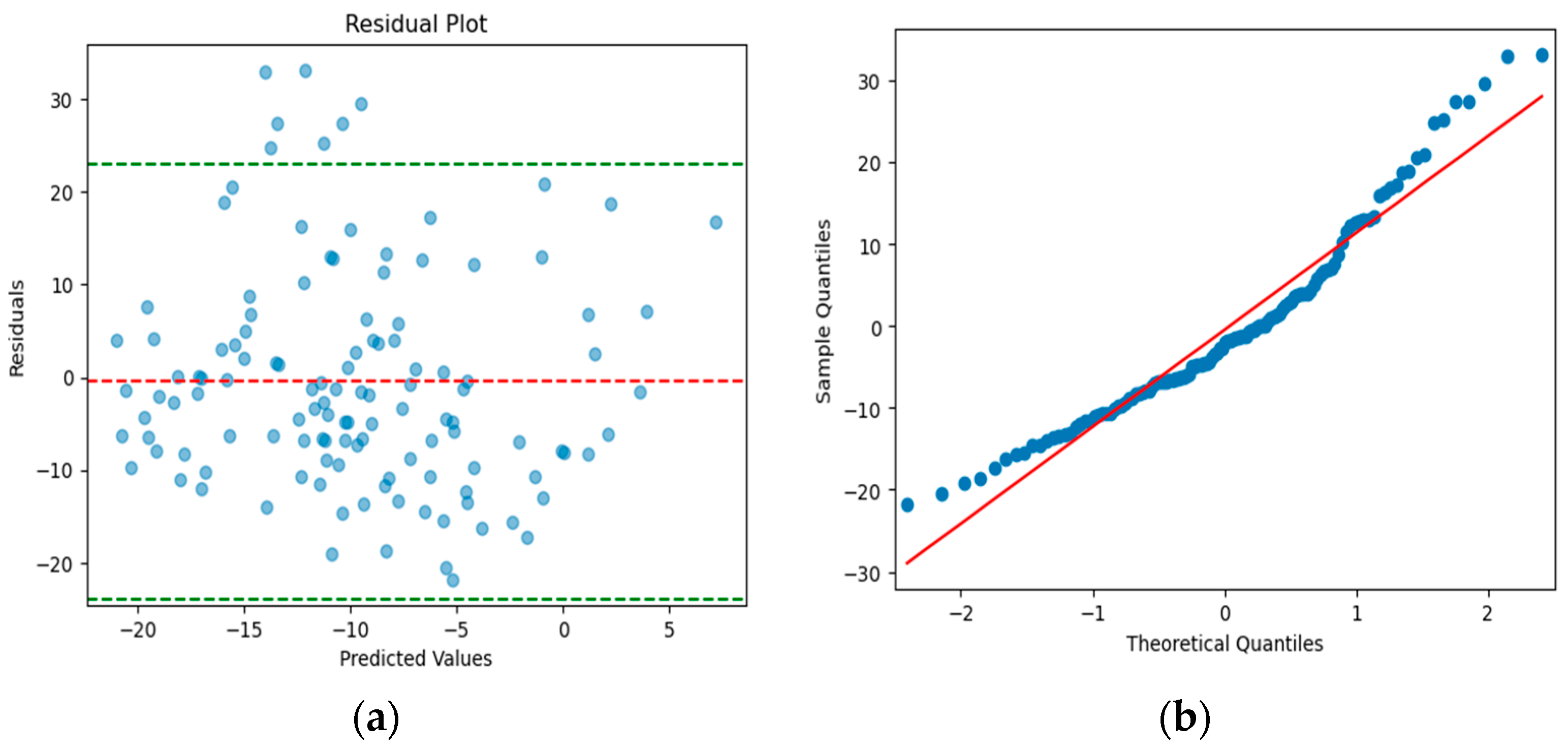
The residual of the MLR model output showed some nonlinearity towards the end, which may have been caused by outliers or a nonlinear relationship between the predictors and the response variable. To address these issues, alternative techniques should be used to further investigate and evaluate the model’s performance. The MLP model did not provide better prediction accuracy, and while it was better at predicting large variations, its performance was inferior to the MLR model for smaller variations. The RMSE was around 10 min and a possible reason could be the unavailability of some dynamic variation in delay and control features in the current independent variables. These variations could be attributed to flight speed changes, weather deviations, or traffic density at terminal areas on a specific day. However, the proposed model is suitable for better resource allocation for round-trip flight times as it outperforms existing models that rely mainly on schedule-based resource allocation.

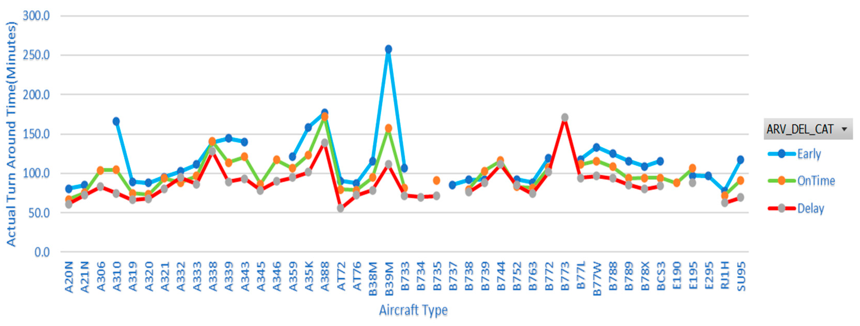
Another notable finding from the analysis was the impact of arrival time variation on actual turnaround process time for various types of aircraft. Figure 9 shows a comprehensive graphical comparison of the average turnaround time for flights to Dubai that arrive early, on schedule, or late. The average turnaround time of scheduled flights operated with all aircraft types arrived in the delay category (“Delay”—delayed more than 15 min from scheduled arrival time) had a shorter time than flights that arrived on time (“OnTime”) and early (“Early”). This implies that in multiple turnaround processes, accurate arrival time prediction has a significant impact on the total turnaround and offers opportunities to optimise existing ground resource planning. Figure 8 shows that the typical turnaround time for the majority of aircraft types ranges between 50 and 100 min. The largest aircraft, the Airbus A388 (largest aircraft), operated from its origin to Dubai with a minimum turnaround time of 114 min and an average turnaround time of 160 min. Another key consideration is that early arrivals to Dubai Airport need a longer actual turnaround time than on-time (“OnTime”) and delayed (“Delay”) arrivals, which can increase ground resource utilisation and lead to delays for other aircraft operating during the same period of operations. This demonstrates the significance of machine learning arrival time prediction for airport ground resource management and planning

Finally, we conducted a comparative case study on resource allocation requirements based on schedule and actual flight arrival time variation for an hour (between 06:00 and 07:00 in Figure 2). There were 15 flights scheduled for that hour, but 18 flights were landed.

Table 7. Comparison of variation of ground resource (manpower) requirements based on scheduled and actual flight movements.

	As Per Scheduled Movement			As Per Actual Flight Movement
Aircraft Type	Flight Count	Manpower/Flight	Total Manpower	Flight Count	Manpower/Flight	Total Manpower
A20N	4	13	52	4	13	52
A320	3	13	39	3	13	39
B38M	3	13	39	4	13	52
B738	3	13	39	3	13	39
B772	1	26	26	1	26	26
B788	1	26	26	1	26	26
A388			0	1	27	27
SU95			0	1	8	8
Total Manpower (ground resource) for the hour			221			269
% of additional manpower required for the hour due to the actual arrival time variation						22%

compares the total manpower required for each aircraft type based on the number of scheduled flights and the actual number of flights landed during the hour.

The ground resource (manpower) required for each aircraft type is based on a hypothetical assumption-based process involved and the number of human resources required in the turnaround process, so the actual manpower requirement per flight in the table may vary slightly based on airline policy and regulatory requirements. Based on the scheduled flight movements, the A20N aircraft type had the largest manpower demand, with 4 flights and a total manpower requirement of 52. The actual flight movements reflect a similar pattern, with the A20N aircraft type having the largest manpower demand with 4 flights and a total manpower requirement of 52. However, there were additional flights that were not accounted for in the scheduled movements, such as 1-A388, 1-B738, and 1-SU95, resulting in a total manpower demand of 269, which is 22% greater than the manpower required based on the scheduled movements. This demonstrates the significance of accurately predicting actual aircraft movements in order to optimise ground resource allocation and minimise inefficiencies.

5. Conclusions

Even though flight schedules are predetermined, flight delays are unavoidable for several reasons, some of which are not human related. These delays cost the aviation industry. One major challenge the aviation industry encounters is early detection of the occurrence of flight delays so that proactive measures can be taken to minimise their impact and costs, especially in ground resource management. We posed an optimisation problem with the goal of optimising the allocation of ground resources at airports by minimising the total number of resources required across all time slots while taking into account the scheduled and actual arrival times of each aircraft type, the maximum number of resources required for each aircraft type, and the availability of resources at each time slot. With the addition of variables that capture variations between scheduled and actual arrivals (arrival delays), the model can robustly optimise ground resource allocation and minimise inefficiencies in airport operations. Based on exploratory data analysis, we assessed the significance of round-trip flight arrival time variation (among 50% of scheduled flights originating from the same airport), hourly arrival count, and ground resource requirements. We proposed a hybrid machine learning model with an exponential moving average to predict arrival delays, especially in round-trip flights. The model was used to calculate reactive arrival delays in aircraft itineraries, which arise as a result of turnaround intervals and arrival delays encountered by flights. To efficiently trace temporal stochastic fluctuations, the proposed model used an exponential moving average of various flight segments. The MLR model has a good fit to the data, as the residuals have a constant variance and are randomly distributed around zero, but the presence of outliers or a nonlinear relationship between the predictors and the response variable could be contributing to the departure from normality observed in the Q-Q plot. In contrast to previous studies [39,40], more accurate and reliable arrival time predictions for multileg flight operations would result in informed decision making and resource planning. The proposed model can predict landing time with an RMSE of 8 min using a minimal number of attributes, making the approach practically feasible for deployment. The model for the classification of arrival time was able to achieve an accuracy of 93.57%. A more accurate arrival time prediction based on machine learning approaches will enable the ground resources management team to optimally deploy resources and establish hourly traffic density well in advance, thus making ground resource optimisation practically feasible. The robustness of the model was validated using various departure destination pairs and diverse types of aircraft. Future research in this area will broaden the current framework to include other complex airport-based characteristics such as runway changes, arrival data, equipment outages, wind speed effect, delay propagation, gate allocation and their effects on departure delay, as well as predict hourly traffic density with fleet mix and estimate ground resource requirements.