Article

Incipient Fault Detection and Reconstruction Using an Adaptive Sliding-Mode Observer for the Actuators of Fixed-Wing Aircraft

1
School of Civil Aviation, Northwestern Polytechnical University, Xi’an 710021, China
2
Shenzhen Research Institute, Northwestern Polytechnical University, Shenzhen 518057, China
*
Author to whom correspondence should be addressed.
Aerospace 2023, 10(5), 422; https://doi.org/10.3390/aerospace10050422
Submission received: 14 September 2022 / Revised: 20 February 2023 / Accepted: 21 March 2023 / Published: 29 April 2023
(This article belongs to the Collection Avionic Systems)

Abstract

:
This paper proposes a new method of detection and reconstruction of the incipient fault of fixed-wing actuators based on an adaptive sliding-mode observer. First, a mathematical model of a fixed-wing aircraft is derived under certain assumptions, considering nonlinear terms and system disturbances. Second, by introducing a nonsingular coordinate transformation, the incipient faults are separated from the disturbances. For a subsystem with no disturbances, the Luenberger observer can estimate the incipient fault. For a subsystem with disturbances, the sliding-mode observer is robust against these disturbances. The Lyapunov stability theory guarantees dynamic error convergence and system stability. The evaluation function was designed to realize residual evaluation and threshold judgment. Third, based on the concept of equivalent output injection, an adaptive sliding-mode observer method is proposed to reconstruct actuator faults precisely under the condition of the uncertain system structure. The design steps of the proposed reconstruction method are introduced in the form of a linear matrix inequality problem, which provides an effective method for calculating the design parameters. Finally, the simulation results of the De Havilland DHC-2 “Beaver” aircraft demonstrate the correctness and effectiveness of the proposed method.

1. Introduction

Fixed-wing unmanned aerial vehicles (UAVs) are widely used in geological mapping, resource surveys, environmental monitoring, meteorological observations, and other fields because of their long flight ranges, large cruising areas, fast flight speeds, and high flight altitudes [1]. However, most UAVs in daily life do not consider fault diagnosis or fault-tolerant control, even if simple fault detection and recovery strategies are applied. These simple strategies cannot effectively ensure the flight safety of UAVs [2]. Fixed-wing UAVs often perform long-term tasks through remote control in poor working environments [3]. In doing so, they are affected by various types of interference and damage, which lead to different faults for these vehicles, such as voltage control faults, actuator lock-in-place physical aging, structural damage, leakage, and fatigue. These faults inevitably affect the performance of UAVs [4]. Therefore, the reliability, stability, and safety of fixed-wing UAV flight are extremely important. Consequently, fault detection of actuators for fixed-wing aircraft has important practical significance and has drawn considerable research attention in recent years [5,6].
In fault detection, abrupt faults have received extensive attention; however, incipient faults have often been ignored [7]. In particular, the incipient faults caused by wear and tear in the mechanical structures of actuators have not been studied thoroughly. If incipient faults are not detected and warnings are not issued in time, these faults may expand and lead to catastrophic consequences [7,8]. Actuator jamming, voltage control faults, structural damage, and other abrupt faults have obvious effects on system performance. Because these abrupt faults are clearly different from disturbances, appropriate thresholds can be selected to detect abrupt faults [9]. Traditional observers, such as unknown input observers, Luenberger observers, and sliding-mode observers (SMOs), can deal with these faults effectively. In a previous study, a sliding-mode control assignment scheme with linear variable parameters was devised for actuator faults. When an actuator fails, the sliding mode first starts and then redistributes control signals to other actuators [10]. Traditional Luenberger observers and SMOs have been designed to manage system uncertainties and abrupt actuator faults [11]. A neural network sliding-mode observer has been designed for the fault detection and estimation of actuators [12]. In linear time-delay systems, adaptive observers are used to detect abrupt actuator faults, and this method can be applied to nonlinear systems [13]. In the case of system interference, extended state observer (ESO) approaches have been devised to detect actuator faults [14]. In the last decade, almost all methods have assumed that the original system is linear, and they have mainly dealt with obvious and serious faults. For the situation in which the system described by the Takagi–Sugeno fuzzy method has a time delay and external disturbance, a fuzzy description learning observer was proposed to realize the simultaneous reconstruction of the system state and an abrupt actuator fault [9,10,11,12,13,14,15]. Higher-order sliding-mode unknown input observers have been proposed to detect abrupt actuator faults and provide the necessary analytical redundancy [16,17]. SMOs are designed to realize the simultaneous detection of actuator faults and sensor faults when the hypothesis is established, whereas an adaptive observer was designed to estimate the sensor faults after the assumptions had been properly relaxed [18]. However, the various methods mentioned above are aimed at abrupt actuator faults. Therefore, it is necessary to detect incipient faults to maintain system stability, which was the inspiration for the present study. In this study, a new adaptive SMO was designed to detect and reconstruct incipient actuator faults.
An incipient fault is a fault that has little impact on the system in the initial stage and can hardly be detected [19]. However, it can grow slowly over time and has a serious impact on the system. Because the effects of faults on the system can be reflected by the symptoms caused by faults, the symptoms caused by faults are divided into significant symptoms and minor symptoms [7,8,20,21]. Incipient faults almost develop gradually in the process of low speed and low frequency, and can hardly be detected in the early stage, which is easy to be covered by the changes of a time-varying process [19,20,21,22]. The term “incipient fault” has two meanings: one refers to the incipient stages of other faults, and the other refers to minor or potential faults that have no obvious symptoms. Timely and effective monitoring of small faults with only minor abnormal signs that may endanger the safe operation of the system is often called incipient fault diagnosis [22]. Generally speaking, according to the time performance of faults, they can be divided into three categories: incipient fault, sudden fault, and intermittent fault [23]. In addition, according to the location of the fault, it can be divided into actuator fault, process fault, and sensor fault. UAVs are often affected by noise, airflow interference, and vibration signals. Regardless of the number of faults or their severity, they start as incipient faults. Because these incipient faults are difficult to find in the initial stage, there have been not a lot of convincing or effective attempts at incipient fault diagnosis in academia. However, incipient faults can cause serious problems, although they develop slowly and are tolerable when they first appear. It seems that it is necessary to detect incipient faults to maintain system stability [23]. UAVs are often affected by noise, airflow interference, and vibration signals. Therefore, it is very difficult to detect and reconstruct incipient faults with disturbances, which was the starting point of this study.
In the past decade, several studies have been conducted on incipient fault detection. Because adaptive fault-tolerant control can reduce the effects of initial faults, a scheme for constructing an unknown input observer was proposed [24]. An incipient fault detection method based on SMO was also presented, which considers physical structure aging [25]. Further, an incipient fault detection method based on neural networks was proposed for a class of nonlinear systems [23]. Inspired by the closed-loop fault diagnosis method [26], an incipient fault detection and estimation method for high-speed trains was introduced [27]. The designs of an SMO and a Luenberger observer for incipient fault detection were described. Under certain conditions, the original system was converted into two subsystems via decoupling. The Luenberger observer was designed for one subsystem with no disturbance, whereas the SMO was designed for the other subsystem with disturbance to ensure the sensitivity of the entire system to the incipient fault. In this scheme, the system residuals were only sensitive to incipient faults; therefore, they could detect faults in a manipulator system [14].
However, the research on incipient fault detection of actuators for fixed-wing UAVs is limited at present. The incipient fault characteristics of such actuators are not obvious, and fixed-wing UAVs are out of the direct control of humans; in addition, their high flight speeds and complex working environments make it difficult to detect incipient faults. Inspired by the previous literature [7,14], this report proposes a correlative robust adaptive SMO to detect and reconstruct incipient actuator faults. By considering the advantages of the combination of an adaptive observer and SMO, the robust detection of incipient faults can be realized, which solves the problem that the previous method [14] cannot reconstruct such actuator faults. This feature represents an innovation of the present study. The main contributions are as follows: First, a nonsingular transformation matrix was designed to decouple an original system with incipient faults and disturbances, and a Luenberger observer and SMO were designed for the decoupled system. The concept of equivalent output injection was introduced into the SMO to estimate the influence of uncertainty on the system. Second, a residual evaluation function was derived for residual evaluation and threshold judgment. Third, based on the uncertainty and unstructured system, an adaptive rate was designed, and the concept of equivalent output error was incorporated to realize actuator fault reconstruction. Finally, the design problem of the adaptive SMO was expressed as a set of linear constraints, which were transformed by the Schur lemma many times and solved by the linear matrix inequality (LMI) technique.
The remainder of this paper is organized as follows: Section 2 describes the mathematical model of a fixed-wing aircraft. Section 3 introduces the robust fault detection and fault reconstruction method of the actuator fault for the system model, proves the stability of the proposed method using Lyapunov analysis, and discusses the accessibility of the designed sliding surface. Section 4 describes some simulation conditions and presents and discusses the mature aircraft model simulations performed in this study. Finally, Section 5 summarizes the conclusions and topics for future work.

2. Problem Formulation

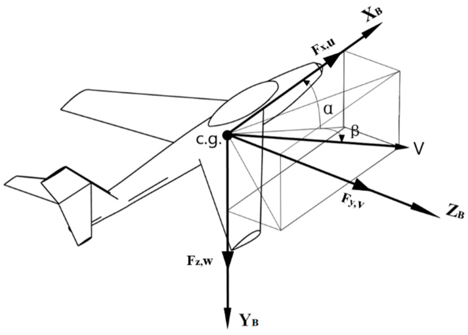
When a fixed-wing aircraft flies in the atmosphere at a high speed, aerodynamic forces and aerodynamic moments are generated owing to the interaction with the air. In addition, under the action of these aerodynamic forces and aerodynamic moments, the gravity and thrust of the aircraft cause elastic deformation of the fuselage, leading to changes in the aerodynamic characteristics of the aircraft. The elastic deformation increases the difficulty of aircraft space motion and flight control technology research. In addition, the mass of the aircraft will change during flight, and the inherent properties of the earth itself will affect the nonlinear and complex relationships among the aircraft aerodynamics, aircraft shape, and flight parameters [28]. For the convenience of this study, the following reasonable assumptions were made.
A fixed-wing aircraft is a complex multi-input multioutput system. By using the six-degree-of-freedom kinematic equation of three centroid motions and three angular motions, the motion state of the aircraft at any moment can be solved. Based on the definitions of the relevant parameters and aircraft coordinates, the aircraft motion is defined by the dynamic equation and motion equation [28]. The equation of state of the aircraft is obtained through many derivations and calculations, including the force, kinematic, moment, and navigation equations presented in (1), (2), (3), and (4), respectively. Figure 1 provides a schematic diagram of the aircraft parameters, and Table 1 lists the respective parameter definitions.
Force equations:
{ u ˙ = v r w q g sin θ + F x m v ˙ = u r + w p + g cos θ sin ϕ + F y m w ˙ = u q v p + g cos θ cos ϕ + F z m
Kinematic equations:
{ θ ˙ = q cos ϕ r sin ϕ ϕ ˙ = p + ( r cos ϕ + q sin ϕ ) tan θ ψ ˙ = 1 cos θ ( r cos ϕ + q sin ϕ )
Moment equations:
{ p ˙ = ( c 1 r + c 2 p ) q + c 3 L ¯ + c 4 N q ˙ = c 5 p r c 6 ( p 2 r 2 ) + c 7 M r ˙ = ( c 8 p c 2 r ) q + c 4 L ¯ + c 9 N
Navigation equations:
{ x ˙ g = V cos μ cos φ y ˙ g = V cos μ sin φ h ˙ = V sin μ
Here,  x = [ u ,   v ,   w ,   ϕ ,   θ ,   ψ ,   p ,   q ,   r ,   x g ,   y g ,   h ] T  is the state vector and  δ = [ δ a ,   δ r ,   δ e ,   δ p ] T  is the control vector. Table A1 (see Appendix A) lists the specific meanings of the aircraft parameters, and Table A2 (see Appendix A) presents the parameter definitions for the dynamic mathematical model. In Table A2, the dimensional derivative parameters of the aircraft can be consulted, and the specific values of these parameters are given in the simulation section. For an aircraft with an actuator fault, the dynamic mathematical models of the longitudinal and lateral directions can be described as follows:
{ x ˙ l d ( l ) ( t ) = A l d ( l ) x l d ( l ) ( t ) + B l d ( l ) u l d ( l ) ( t ) + D l d ( l ) f a ( t ) y l d ( l ) ( t ) = C l d ( l ) x ( t )
In this study, the system satisfied the Lipschitz condition. Under the simultaneous influence of the nonlinear term and system disturbance, the system differential equation can be expressed as follows:
{ x ˙ ( t ) = A x ( t ) + B u ( t ) + ξ ( x , t ) + D f a ( t ) + E ψ ( t ) y ( t ) = C x ( t )
where  { x l d ,   x l } x R n { u l d ,   u l } u R n , and  y R n  are the system state, input vector, and output vector, respectively, and  { A l d ,   A l } A { B l d ,   B l } B { C l d ,   C l } C , and  { D l d ,   D l } D  are known matrices. The pair  ( A ,   C )  is observable.  C  and  E  are the known constant matrix with full rank, respectively;  ξ ( x , t )  is the known nonlinear continuous term;  f a = [ f a 1 ,   f a 2 ,   ,   f a m ] T  is the actuator fault; and  ψ ( t )  represents the lumped uncertainties and disturbances experienced by the system.
Assumption 1.
The known nonlinear term,  ξ ( x , t ) , satisfies the Lipschitz condition in  x , and  γ  is the known Lipschitz constant.
ξ ( x , t ) ξ ( x ^ , t ) γ x x ^ ,   x , x ^ n
Assumption 2.
f a  satisfies the following constraints:
f a ρ a   and   ψ ( t )
Assumption 3.
r a n k ( C E ) = r a n k ( E ) .
Under the previous assumptions, two nonsingular matrices can be found to decouple the system. After applying transformation matrices, system (6) can be changed into the following two subsystems:
{ x ˙ 1 = A 1 x 1 + A 2 x 2 + 1 ξ 1 ( 1 x , t ) + B 1 ( u + f a ) + E 1 ψ y 1 = C 1 x 1
{ x ˙ 2 = A 3 x 1 + A 4 x 2 + 2 ξ 2 ( 1 x , t ) + B 2 ( u + f a ) y 2 = C 4 x 2
where  = [ 1 2 ] T  and  = [ 1 2 ] T  are the nonsingular matrices.  A 11 R r × r A 2 R r × ( n r ) A 3 R ( n r ) × r A 4 R ( n r ) × ( n r ) B 1 R r × m B 2 R ( n r ) × m C 1 R r × r C 4 R ( p r ) × ( n r ) x = [ x 1 x 2 ] T x 1 R r x 2 R n r ξ 1 R r ξ 2 R n r y = [ y 1   y 2 ] y 1 R r y 2 R p r .
The matrix transformations in (9) and (10) are formulated as follows [29]:
A 1 = [ A 1   A 2 A 3   A 4 ] ,   B = [ B 1 B 2 ] ,   C 1 = [ C 1 0 0 C 4 ] ,   E = [ E 1 0 ] .
Remark 1.
System (9) has both actuator faults  f a  and unknown disturbances  ξ , whereas (10) only includes actuator faults  f a  without unknown disturbances  ξ . The system can be decoupled through such transformations.

3. Adaptive Robust Fault Detection and Reconstruction Method

This section presents the design of the proposed robust fault reconstruction method for the actuator faults of fixed-wing aircraft. First, a synthetic observer was designed for the interference estimation and fault detection of the unknown system. An adaptive SMO was proposed to address the problems of fault detection and reconstruction. The fault signals were accurately reconstructed using the concept of equivalent output injection. Second, considering that the system structure cannot be completely decoupled from a fault, the reconstruction method of the actuator fault (RAF) was constructed to estimate the state quantity and faults. The stability of the observer was analyzed using an LMI solution. Finally, an actuator fault reconstruction approach was developed to reconstruct the actuator fault and all state quantities. Figure 2 shows the diagnosis block diagram.

3.1. Actuator Fault Detection

The detection of actuator faults (DAF) is the first step in determining if a fault has occurred. When a significant change in residuals is observed, it is possible that a fault has occurred. If the adaptive state estimator is directly designed for the original system, when the gain of (13) is significantly large, the residual will be within the chattering range or below the preset threshold. Therefore, incipient actuator fault detection is difficult. By analyzing the two subsystems after the transformation matrix, a synthetic observer comprising SMOs and the Luenberger observer was constructed in this section to simultaneously detect faults and estimate disturbances.

3.1.1. SMO Design

Assumption 4.
The minimum phase condition (see [30]).
Lemma 1.
In the case of Assumption 4, pair (A4, C4) is detectable, and there exist matrices L0, such that  A 4 L 0 C 4  is stable; furthermore, the following Lyapunov equation is applicable [31]:
( A 4 L 0 C 4 ) T P 0 + P 0 ( A 4 L 0 C 4 ) = Q 0
where  P 0   and   Q 0  are symmetric positive definite matrices.
For (9), the proposed SMO is designed as follows:
{ x ^ ˙ 1 = A 1 x ^ 1 + A 2 x ^ 2 + ξ 1 ( T 1 x ^ , t ) + B 1 u + w 1 + ( A 1 A 1 s ) C 1 1 ( y 1 y ^ 1 ) y ^ 1 = C 1 x ^ 1
where  A 1 s R r × r  and  w 1  can be defined by
w 1 = { ( E 1 + η 1 ) P 1 ( x 1 x ^ 1 ) P 1 ( x 1 x ^ 1 ) if x 1 x ^ 1 0 0   if x 1 x ^ 1 = 0
where  η 1  is a positive scalar, determined using (28), and  P 1  is the Lyapunov matrix of  A 1 s .
For (10), the proposed observer is:
{ x ^ ˙ 2 = A 4 x ^ 2 + A 3 x ^ 1 + ξ 2 ( T 1 x ^ , t ) + B 2 u + L 0 ( y 2 y ^ 2 ) y ^ 2 = C 4 x ^ 2
where L0 is the gain of the Luenberger observer.
Based on (12) and (14), the corresponding error dynamic equations can be expressed as follows:
e ˙ 1 = x ˙ 1 x ^ ˙ 1 = A 1 s e 1 + A 2 e 2 + ξ 1 ( T 1 x , t ) ξ 1 ( T 1 x ^ , t ) + E 1 ψ w 1
e ˙ 2 = x ˙ 2 x ^ ˙ 2 = ( A 4 L 0 C 4 ) e 2 + ξ 2 ( T 1 x , t ) ξ 2 ( T 1 x ^ , t )

3.1.2. Stability Analysis

Proposition 1.
If there are matrices  A 1 s < 0 P 0 = P 0 T > 0 P 1 = P 1 T > 0 , and  α 1   and   α 2  satisfy (17), the error dynamics are asymptotically stable:
Λ : = [ Π 1 + 1 α 1 P 1 P 1 P 1 A 2 A 2 T P 1 Π 2 + 1 α 2 P 0 P 0 + a I n r ] < 0
where  Π 1 = A 1 s T P 1 + P 1 A 1 s α 1 > 0 ,   α 2 > 0 ,   Π 2 = ( A 4 L 0 C 4 ) T P 0 + P 0 ( A 4 L 0 C 4 ) a = α 1 γ f 1 2 1 2 + α 2 γ f 2 2 1 2 .
Proof of Proposition 1.
From (15), V1 becomes
V ˙ 1 = e ˙ 1 T P 1 e 1 + e 1 T P 1 e ˙ 1 = e 1 T ( A 1 s T P 1 + J 1 A 1 s ) e 1 + 2 e 1 T P 1 ( ξ 1 ( 1 x , t ) ξ 1 ( 1 x ^ , t ) ) + 2 e 1 T P 1 E 1 ψ + 2 e 1 T P 1 A 2 e 2 2 e 1 T P 1 w 1
Similarly, the derivative of V2 together with (16) can be obtained:
V ˙ 2 = e ˙ 2 T P 0 e 2 + e 2 T P 0 e ˙ 2 = e 2 T ( P 0 ( A 4 L 0 C 4 ) + ( A 4 L 0 C 4 ) T P 0 ) e 2 + 2 e 2 T P 0 ( ξ 2 ( 1 x , t ) ξ 2 ( 1 x ^ , t ) )
From (13), it is easy to obtain  e 1 T J 1 w 1 = ( E 1 + η 1 ) J 1 e 1 .
Therefore, under Assumption 1,
2 e 1 T P 1 E 1 ψ 2 E 1 ψ P 1 e 1 2 E 1 P 1 e 1
Thus, (1), (18) and (19) can be respectively simplified as follows:
V ˙ 1 e 1 T 1 e 1 + 1 α 1 e 1 T P 1 P 1 e 1 + α 1 γ ξ 1 2 1 2 e 2 2 + 2 e 1 T P 1 A 2 e 2 2 η 1 P 1 e 1 e 1 T ( 1 + 1 α 1 P 1 P 1 ) e 1 + α 1 γ ξ 1 2 1 2 e 2 2 + 2 e 1 T P 1 A 2 e 2
V ˙ 2 = e 2 T P 0 e ˙ 2 + e ˙ 2 T P 0 e 2 e 2 T ( 2 + 1 α 2 P 0 P 0 ) e 2 + α 2 γ ξ 2 2 1 2 e 2 2
Then, combining (21) and (22), we can obtain:
V ˙ = V ˙ 1 + V ˙ 2 e 1 T ( 1 + 1 α 1 P 1 P 1 ) e 1 + e 2 T ( 2 + 1 α 2 P 0 P 0 + a I n r ) e 2 + 2 e 1 T P 1 A 2 e 2 = [ e 1 e 2 ] T Λ [ e 1 e 2 ]
From Proposition 1, it can be deduced that  [ e 1 e 2 ] T 0  and  V ˙ < 0 ; furthermore, the error dynamics in (15) and (16) are asymptotically stable.
Therefore, Proposition 1 shows that the error dynamics system is asymptotically stable. Because (17) is not easy to solve directly using MATLAB, it can be changed into the LMI feasibility problem in (24) by using the Schur complement [32]:
[ X + X T P 1 P 1 A 2 0 P 1 α 1 I 0 0 A 2 T P 1 0 N P 2 0 0 P 0 α 2 I ] < 0
where  N = A 4 T P 0 + P 0 A 4 C 4 T Y T Y C 4 + a I X = P 1 A 1 s , and  Y = P 0 L 0 , and  α 1   and   α 2  are positive scalars. □

3.1.3. Reachability Condition Analysis

In (16),  e 2 ( t )  can be written as
e 2 ( t ) = 0 t e ( A 4 L 0 C 4 ) ( t τ ) ( ξ ( x , t ) ξ ( x ^ , t ) ) d τ + e ( A 4 L 0 C 4 ) t e 0 ( 0 ) c 0 γ ξ 2 1 0 t e b 0 ( t τ ) e 2 ( τ ) d τ + c 0 e b 0 t e 2 ( 0 )
where  b 0   and   c 0  can be obtained using  e ( A 4 L 0 C 4 ) t c 0 e b 0 t Λ = A 4 L 0 C 4 . Applying the Gronwall–Bellman inequality [33] to (25) yields
e 2 ( t ) c 0 e 2 ( 0 ) e ( c 0 γ ξ 2 1 b 0 ) t
The sliding-mode surface is
ς = { ( e 1 , e 2 ) | e 1 = 0 }
Proposition 2.
If the LMI formulated in (24) is solvable and the gain  η 1  is expressed as in (28), the state error dynamics (15) and (16) can be driven to the sliding-mode surface:
η 1 ( A 2 + γ ξ 1 1 ) ε + η 2
Proof of Proposition 2.
(18)(1) is written as follows under Assumption 2:
V ˙ 1 2 P 1 e 1 A 2 e 2 + 2 P 1 e 1 E 1 + 2 P 1 e 1 γ ξ 1 1 e 2 2 P 1 e 1 ( E 1 + η 1 ) 2 P 1 e 1 ( ( A 2 + γ ξ 1 1 ) e 2 η 1 ) 2 η 2 P 1 e 1 2 η 2 V 1 λ min ( P 1 )
Therefore, (29) satisfies the reachability condition [4].
When the fault occurs at time  t f e ˙ 2  becomes
e ˙ 2 = ( A 4 L 0 C 4 ) e 2 + ( ξ 2 ( 1 x , t ) ξ 2 ( 1 x ^ , t ) ) + B 2 f a
In general, it can be simply determined whether a fault occurs by comparing the residual characteristics with the threshold value. In this study, we used the following logical relationships to determine the occurrence of faults:
J r ( t ) J t h f a u l t   occurs     alarm
J r ( t ) < J t h   no   f a u l t   occurs     no   alarm
J r ( t ) = [ t t + T 1 r T ( t ) r ( t ) d t ] 1 2
where the residual signal  r  can be expressed as  y y ^ J r ( t )  is the residual evaluation function, and  T 1  is the evaluation time window of finite length. □
Proposition 3.
For the nonlinear faulty system in (9) and (10), the above evaluation function,  J r ( t ) , and observer (12), when  J r ( t )  exceeds  J t h , the occurrence of a fault can be determined. The threshold,  J t h , can be expressed as follows:
J t h = [ t t + T 1 ( k ( η ¯ + L D ψ ¯ 1 ) C λ k γ + ( k ε k ( η ¯ + L D ψ ¯ 1 ) c 0 b 0 γ 1 ) C e ( c 0 b 0 γ ) τ + D ψ ¯ 1 ) 2 d τ ] 1 2
where  b 0   and   c 0  can be obtained from (26) and  ε  is a constant bound.
Proof of Proposition 3.
Under Assumptions 1–3, applying the triangle inequality, the upper bound on the norm of x can be written as follows:
x ˙ ( t ) e Λ t x ˙ ( 0 ) + 0 t e Λ ( t τ ) ξ ( x , t ) ξ ( x , t ) + L ψ d τ e Λ t x ˙ ( 0 ) + 0 t e Λ ( t τ ) ( f ( x ( τ ) , u ( τ ) ) f ( x ^ , t )   + L ψ ) d τ e Λ t ε + γ 0 t e Λ ( t τ ) x ( τ ) x ^ ( τ ) d τ + ( L ψ ¯ 1 ) 0 t e Λ ( t τ ) d τ e Λ t ε + γ 0 t e Λ ( t τ ) x ( τ ) x ^ ( τ ) d τ + ( L ψ ¯ 1 ) 0 t e Λ ( t τ ) d τ
Using (26), (35) has the following form:
x ˙ ( t ) b 0 c 0 e λ t + b 0 γ 0 t x ˙ ( τ ) e λ ( t τ ) d τ + b 0 L ψ ¯ 1 λ ( 1 e λ t )
Considering (9), the residual signal  r  can be obtained. Therefore, based on the selected evaluation function in (31), the evaluation threshold is as follows:
J th = [ t t + T 1 ( k ( η ¯ + L D ψ ¯ 1 ) C λ k γ + ( k ε k ( η ¯ + L D ψ ¯ 1 ) c 0 b 0 γ 1 ) C e ( c 0 b 0 γ ) τ + D ψ ¯ 1 ) 2 d τ ] 1 2
It should be noted that this is a worst-case estimate of the possible effects of the estimation error norm in the fault-free case. □
Remark 2.
From Lemma 1,  J r ( t )  is close to zero before an actuator fault occurs. Based on (26) and (30),  J r ( t ) is treated as a residual to detect actuator faults. From (26), when (6) is healthy,  J r ( t )  tends to be zero. However, when (6) has actuator faults, a threshold,  J t h , can be selected. After fault detection and alarm signals were generated, an adaptive reconstruction strategy was initiated to reconstruct the unknown fault. Table 2 summarizes the steps of actuator fault diagnosis.

3.2. Actuator Fault Reconstruction

This section describes the actuator fault reconstruction performed after DAF. The difference between the reconstruction actuator method and most fault diagnoses is that the reconstruction actuator method can detect and isolate actuator faults and provide detailed information regarding them. Therefore, it is particularly suitable for incipient fault diagnosis, which is difficult to detect. In this section, when the system uncertainty is unstructured, a new adaptive SMO-based reconstruction actuator method can be designed.
When the system uncertainty is unstructured, (6) can be expressed as
{ x ˙ ( t ) = A x ( t ) + B u ( t ) + ξ ( x , t ) + D f a ( t ) + ψ ( t ) y ( t ) = C x ( t )
Assume that  A = [ A 1 A 2 A 3 A 4 ] , D = [ D 1 D 2 ] , and if  C = [ 0   I p ] , it is possible to find a nonsingular transformation matrix as follows:
T c = [ N c T   C ] T
In doing so,  C T c 1 = [ 0   I p ] N c R n × ( n p ) , and the columns span the null space of C.
Assumption 5.
The matrix pair (A, C) is detectable, such that A-LC is stable; thus, for any M > 0, the Lyapunov equation in (40) has a unique solution S > 0:
( A L C ) T J + J ( A L C ) = M
where  J = [ J 1 J 2 J 2 T J 3 ]   and   M = [ M 1 M 2 M 2 T M 3 ] .
Assumption 6.
There is an arbitrary matrix F that satisfies the equation
D T J = F C
Lemma 2.
Under Assumptions 5 and 6, the following two equations can be obtained [34]:
(a)  D 1 + J 1 1 J 2 D 2 = 0  (b)  A 1 + J 1 1 J 2 A 3  is stable.

3.2.1. SMO Design

By introducing a transformation matrix in this form,  U = [ U 1 U 2 ] = [ I n p J 1 1 J 2 0 I p ] , (38) can be changed into the system:
{ x ˙ ( t ) = A U x ( t ) + U ξ ( U 1 x , t ) + B U u ( t ) + U ψ ( t ) + D U f a ( t ) y ( t ) = C U x ( t )
where
A U = [ A ¯ 1 A ¯ 2 A ¯ 3 A ¯ 4 ] = [ A 1 + J 1 1 J 2 A 3 A 2 A 1 J 1 1 J 2 + J 1 1 J 2 ( A 4 A 3 J 1 1 J 2 ) A 3 A 4 A 3 J 1 1 J 2 ]
B U = [ B ¯ 1 B ¯ 2 ] = [ B 1 + J 1 1 J 2 B 2 B 2 ]
D U = [ D ¯ 1 D ¯ 2 ] = [ D 1 + J 1 1 J 2 D 2 D 2 ] = [ 0 D 2 ]
C U = [ 0 I p ]
System (42) can further be expressed as follows:
{ x ˙ 1 = A ¯ 1 x 1 + A ¯ 2 x 2 + U 1 ξ ( T 1 x , t ) + B ¯ 1 u ( t ) + U 1 ψ ( t ) x ˙ 2 = A 3 z 1 + A ¯ 4 z 2 + U 2 ξ ( T 1 x , t ) + B ¯ 2 u ( t ) + D 2 f a + U 2 ψ ( t ) y = x 2
For (47), the SMO can be constructed as follows:
{ x ^ ˙ 1 = A ¯ 1 x 1 + A ¯ 2 y + U 1 ξ ( T 1 x ^ , t ) + B ¯ 1 u ( t ) x ^ ˙ 2 = A 3 z 1 + A ¯ 4 z 2 + U 2 ξ ( T 1 x ^ , t ) + B ¯ 2 u ( t ) + ( A ¯ 4 A 0 ) ( y y ^ ) + w 3 y ^ = x ^ 2
and
w 3 = { ( D 2 ρ a + η 1 ) J 0 ( y y ^ ) J 0 ( y y ^ ) + δ if   y y ^ 0 0 if   y y ^ = 0
where  δ  is a small positive scalar that reduces the effect of chattering.  η 1  is a positive scalar, and J0 is a symmetric positive-definite matrix.
By defining the state estimation errors,  e 1 = x 1 x ^ 1  and  e 2 = x 2 x ^ 2 , based on (47) and (48), the corresponding error dynamic equations can be written:
e ˙ 1 = A ¯ 1 e 1 + U 1 ( ξ ( U 1 x , t ) ξ ( U 1 x ^ , t ) ) + U 1 ψ
e ˙ 2 = A 0 e 2 + A 3 e 1 + U 2 ( ξ ( U 1 x , t ) ξ ( U 1 x ^ , t ) ) + D 2 f a + U 2 ψ w 3

3.2.2. Stability Analysis

Proposition 4.
For (42), under Assumptions 1, 2, 5, and 6, if  J 0 = J 0 T > 0 ,  J 1 = J 1 T > 0 ,  A 0 ,  Y ,  Z ,  ν , and positive scalars  α 1   and   α 0  satisfy (51) and (52), and the LMI feasibility problem has the solution in (54). With the prescribed  H  disturbance attenuation level  μ > 0 , the error dynamics is asymptotically stable:
J 1 D 1 + J 2 D 2 = 0
[ Θ 1 + I n p A 3 T J 0 J 1 J 2 J 0 A 3 Θ 2 + I p 0 J 0 J 1 0 μ I n p 0 J 2 T J 0 0 μ I p ] < 0
[ Θ 3 A 3 T J 0 Z G 1 Z G 2 Z G 1 Z G 2 0 J 0 A 3 Θ 4 0 J 0 0 0 J 0 G 1 T Z T 0 μ I n p 0 0 0 0 G 2 T Z T P 0 0 μ I p 0 0 0 G 1 T Z T 0 0 0 α 1 I n p 0 0 G 2 T Z T 0 0 0 0 α 1 I p 0 0 J 0 0 0 0 0 α 0 I p ] < 0
H : = sup ψ 2 0 e 2 ψ 2 μ
The adaptive fault estimation algorithm is given by
f ^ ˙ = ν F C ¯ 1 e 1
where
Θ 1 = A 1 T J 1 + J 1 A 1 + A 3 T J 2 T + J 2 A 3 + 1 α 1 ( J 1 J 1 + J 2 J 2 T ) + ( α 1 + α 0 ) γ ξ 2 I n p
Θ 2 = A 0 T J 0 + J 0 A 0 + 1 α 0 J 0 J 0
Θ 3 = A 1 T G 1 T Z T + Z G 1 A 1 + A 3 T G 2 T Z T + Z G 2 A 3 + ( α 1 + α 0 ) γ f 2 I n p + I n p
Θ 4 = Y + Y T + I p
G 1 = ( I n D D + ) [ I n p 0 ] ,   G 2 = ( I n D D + ) [ 0 I p ] ,   D + = ( D T D ) 1 D T
where  D +  is the generalized inverse of D. The linear matrix equality in (52) is difficult to solve directly, so it becomes a minimization problem [35].
In actuator fault reconstruction, the adaptive method in (54) is proposed to solve the problem and to obtain an accurate solution.
Proof of Proposition 4.
From (52),  D 1 + J 1 1 J 2 D 2 = 0  is equivalent to (50) and can be written as follows:
[ J 1 J 2 ] D = 0
Under  r a n k [ D 0 ] = r a n k [ D ] , (62) can be rewritten as
[ J 1 J 2 ] = Ω ( I n D ( D T D ) 1 D T )
where  Ω  denotes the design matrix. Substituting  J 1 = Ω ( I n D D + ) [ I n p 0 ]  and  J 2 = Ω ( I n D D + ) [ 0 I p ]  into (53) and using the Schur complement, (54) can be proven.
For the following function:
V = V 1 ( e 1 ) + V 2 ( e 2 ) = e 1 T J 1 e 1 + e 2 T J 0 e 2
where  J x = [ J 1 0 0 J 0 ]  is a new coordinate and  J 0 = J 2 T J 1 T J 2 + J 3 .
Combined with (50), the time derivative of V1 can be expressed as follows:
V ˙ 1 = e ˙ 1 T J 1 e 1 + e 1 T J 1 e ˙ 1 = 2 e 1 T J 1 U 1 ( ξ ( U 1 x , t ) ξ ( U 1 x ^ , t ) ) + e 1 T ( A ¯ 1 T J 1 + J 1 A ¯ 1 ) e 1 + 2 e 1 T J 1 U 1 ψ
Similarly, the derivative of V2 together with (51) can be written as
V ˙ 2 = e ˙ 2 T J 0 e 2 + e 2 T J 0 e ˙ 2 = 2 e 2 T J 0 U 2 ( ξ ( U 1 x , t ) ξ ( U 1 x ^ , t ) ) + e 2 T ( A 0 T J 0 + J 0 A 0 ) e 2 + 2 e 2 T J 0 A 3 e 1 + 2 e 2 T J 0 D 2 f a + 2 e 2 T J 0 U 2 ψ 2 e 2 T J 0 w 3
As the forms
U 1 [ x y ] U 1 [ x ^ y ] = U 1 [ e 0 ] = e
and
ξ ( U 1 x , t ) ξ ( U 1 x ^ , t ) γ ξ e
exist, if  ε > 0 ,    then
2 X T Y 1 ε X T X + ε Y T Y
Combining (65)–(68), it has
V ˙ = V ˙ 1 + V ˙ 2 = e 1 T 1 e 1 + e 2 T 2 e 2 + 2 e 2 T J 0 A 3 e 1 + 2 e 1 T J 1 U 1 ψ + 2 e 2 T J 0 U 2 ψ
If  ψ = 0 , then
V ˙ [ e 1 e 2 ] T [ Θ 1 A 3 T J 0 J 0 A 3 Θ 2 ] [ e 1 e 2 ]
Under (53), if  [ Θ 1 A 3 T J 0 J 0 A 3 Θ 2 ] < 0 , then  V ˙ < 0 ; that is, when  t 0 ,   e 0 .
If  ψ 0 , to achieve robustness to disturbance, the performance index can be introduced [36]:
Γ = 0 ( e 2 μ ψ 2 ) d t
As  V ( ) > 0 V ( 0 ) = 0 . Then, (72) becomes
Γ = 0 ( e 2 μ ψ 2 + V ˙ ) d t 0 V ˙ d t   0 ( [ e 1 e 2 ψ ] T [ 1 0 0 0 1 0 0 0 μ ] [ e 1 e 2 ψ ] ) d t
Under (53), then  Γ < 0 ; that is,  e 2 μ ψ 2 . Therefore, the detection indicator has been constructed. □

3.2.3. Reachability Condition Analysis

The sliding-mode surface is defined for the error dynamics (50) and (51) as follows:
ς = { ( e 1 , e 2 ) | e 2 = 0 }
Proposition 5.
For the designed observer (48), if the LMI formulated in (54) and gain  η 1  from (49) Error! satisfying (75) are solvable, the state error dynamics in (50) and (51) can be driven to the sliding-mode surface in finite time and remain on it:
η 1 A 3 ε + γ ξ ε + χ + η 2
where  e ε  and  η 2  is a scalar.
Proof of Proposition 5.
For the Lyapunov candidate function as  W ( e 2 ) = e 2 T J 0 e 2 , the derivative of the Lyapunov function  W  with respect to time is as follows:
W ˙ = e 2 T ( A 0 T J 0 + J 0 A 0 ) e 2 + 2 e 2 T J 0 A 3 e 1 + 2 e 2 T J 0 U 2 ( ξ ( U 1 x , t ) ξ ( U 1 x ^ , t ) ) + 2 e 2 T J 0 D 2 f a + 2 e 2 T J 0 U 2 ψ 2 e 2 T J 0 w 3
As  A 0 T J 0 + J 0 A 0 < 0 e ε , can be written as
W ˙ 2 e 2 T J 0 A 3 e 1 + 2 e 2 T J 0 U 2 ( ξ ( U 1 x , t ) ξ ( U 1 x ^ , t ) ) 2 ( D 2 ρ a + η 1 ) J 0 e 2 + 2 e 2 T J 0 D 2 f a + 2 e 2 T J 0 U 2 ψ 2 J 0 e 2 ( A 3 e 1 + γ f e 1 + D 2 ρ a + χ D 2 ρ a η 1 = 2 J 0 e 2 ( A 3 ε + γ f ε + χ η 1 )
If (75) exists, then  W ˙  can be expressed as
W ˙ 2 η 2 J 0 e 2 2 η 2 W λ min ( J 0 )
where  λ min ( J 0 )  is the smallest eigenvalue of  J 0 .
Under Proposition 5, a sliding motion is achieved and  e 2 = e ˙ 2 = 0  represents perfect sliding. The error dynamics in (51) can be rewritten as (79). Because the discontinuous vector in (49) can only be approximated, the error dynamics cannot slide perfectly on surface  ς  [28,37]:
0 = A 3 e 1 + U 2 ( ξ ( U 1 x , t ) ξ ( U 1 x ^ , t ) ) + D 2 f a + U 2 ψ w 3 e q
where  w 3 e q  is the equivalent output error injection.
Define  f ^ a = D 2 + w 3 e q . Then, (79) can be expressed as
f a f ^ a = D 2 + U 2 ( ξ ( U 1 x , t ) ξ ( U 1 x ^ , t ) ) D 2 + A 3 e 1 D 2 + U 2 ψ
As  e 2 μ ψ 2 , computing the norm of (80) yields
f a f ^ a 2 ( μ σ max ( D 2 + A 3 ) + μ r f σ max ( D 2 + ) + σ max ( D 2 + ) ) ψ 2 = ( μ β 1 + β 2 ) ψ 2
where  β 1 = σ max ( D 2 + A 3 ) + r f σ max ( D 2 + )  and  β 2 = σ max ( D 2 + ) .
If there is a small  Δ = ( μ β 1 + β 2 ) ψ 2 , then  f ^ a  can be written as
f ^ a = k ν D 2 + J 0 ( y y ^ ) J 0 ( y y ^ ) + δ
where  ν  is the adaptive rate,  β 1 = σ max ( D 2 + A 3 ) + γ ξ σ max ( D 2 + ) , and  β 2 = σ max ( D 2 + ) . □
From (64), the actuator fault estimation is related to the system uncertainties and  Δ . Generally, it is impossible to accurately estimate actuator faults in the presence of unknown disturbances. However, when  μ  is sufficiently small, the proposed method can effectively maintain the shape of the fault signal. By minimizing  μ , the robustness of the proposed observer to the unknown signal can be enhanced, and the ideal accuracy of the fault estimation can finally be obtained. Table 3 summarizes the steps of actuator fault reconstruction.
In the following section, a simulation is used to verify the performance of the proposed method. It is worth noting that the simulation in this study uses the longitudinal model of fixed-wing aircraft, and this method is also applicable to the lateral model of fixed-wing aircraft, so the method proposed in this paper is universal.

4. Simulation Results

This section may be divided by subheadings. It should provide a concise and precise description of the experimental results, their interpretation, and the experimental conclusions that can be drawn.
As shown in Figure 3, a De Havilland DHC-2 “Beaver” aircraft with Air Canada number 1244 was used as the simulation object to verify the overall performance of the proposed adaptive fault detection and fault reconstruction method [
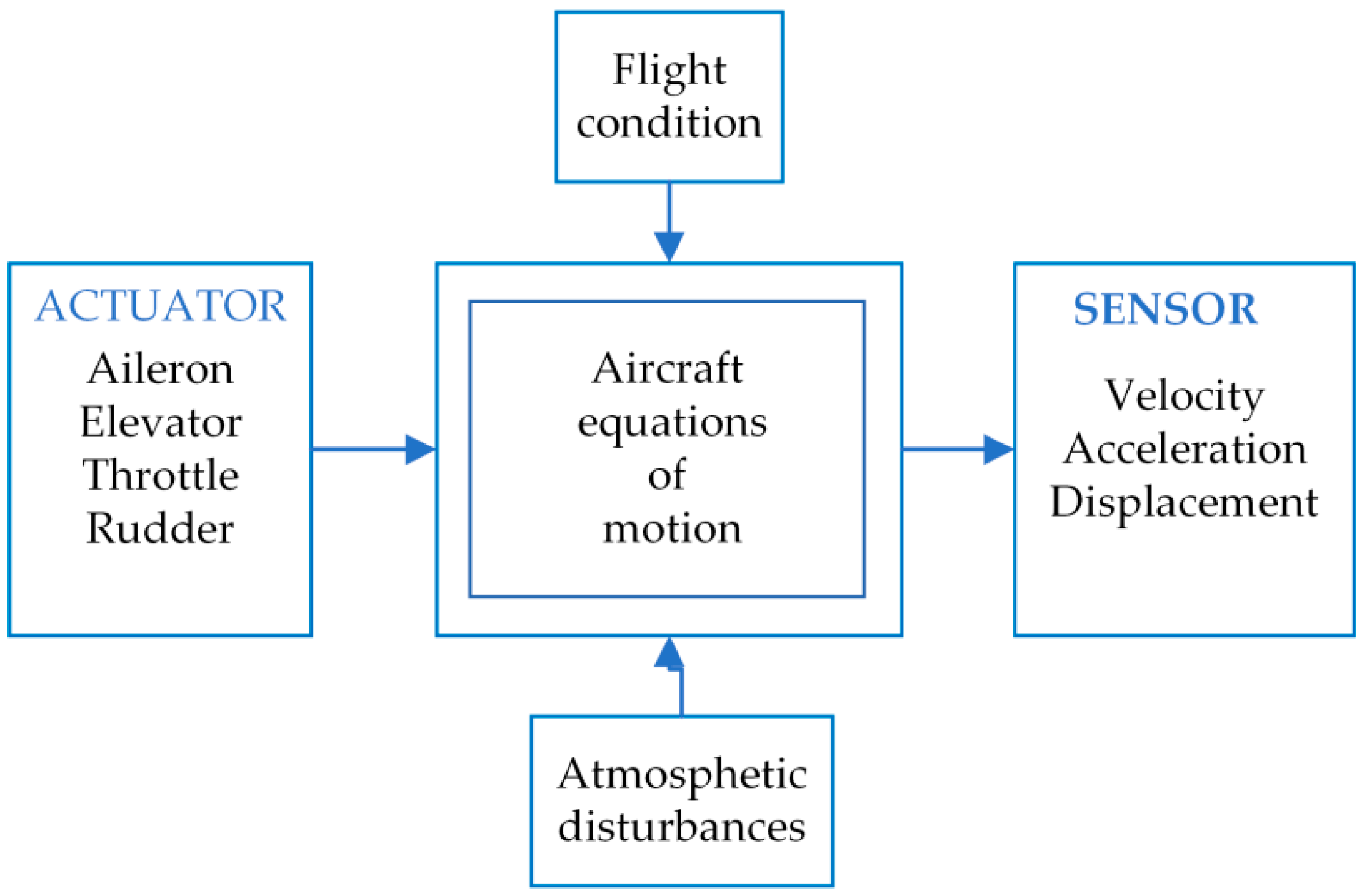
38]. Fixed-wing aircraft have been extensively studied from flight control design to fault reconstruction. Under certain flight conditions and disturbances, the control response relation of the aircraft motion equation includes the actuator of the input unit and the sensor of the output unit. Thus, the importance of actuator fault diagnosis and reconstruction is critical. Figure 4 shows the basic control–response relationship for “Beaver”, and Table 4 lists the relevant parameter values.
The dimensional derivative parameters of the aircraft are as follows:  L p = 5.4022 L δ α = 7.2976 M q = 3.0292 X α = 5.4534   M δ e = 10.6 X v = 0.0389 X δ T = 0.7489 N r = 0.552 , and  N δ r = 2.6058 . Using this model, the correlation coefficient matrix was calculated to be
A l = [ 0 . 0384 5.4145 0.4084 9.7766 0.0085 1.2882 0.9764 0.0022 0.0124 6.7753 3.0292 0 0 0 1 0 ]
B l = [ 0.7271 1.6888 0.1104 0.3645 10.6009 2.2471 0 0 ] C l = [ 1 0 0 0 0 1 0 0 0 0 1 0 0 0 0 1 ]
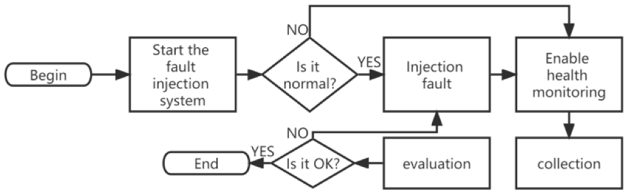
After selecting the faults to be injected from the failure mode library, the fault injection experiment is started. The experimental procedure is as shown in 
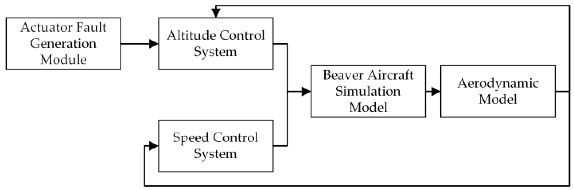
Figure 5. To simulate faults, a flight control simulation model was designed, as shown in Figure 6.
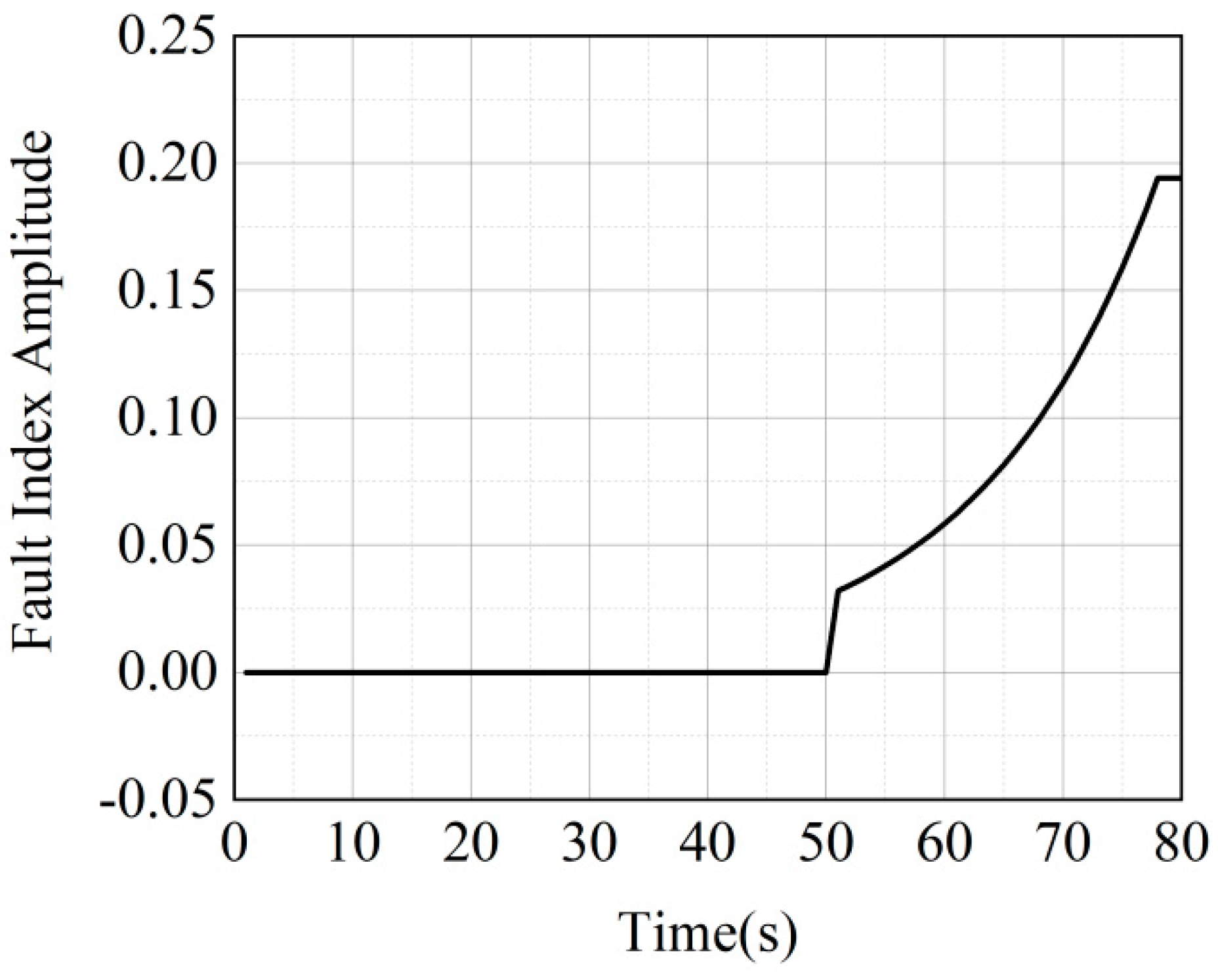
The simulation module consists of four parts: a longitudinal linearization model of an aircraft, an altitude control unit with a stability enhancement algorithm, a speed control unit, and a fault simulation module. The microvariation of the control input on the elevator drive motor involved in simulation case 1 is shown in 
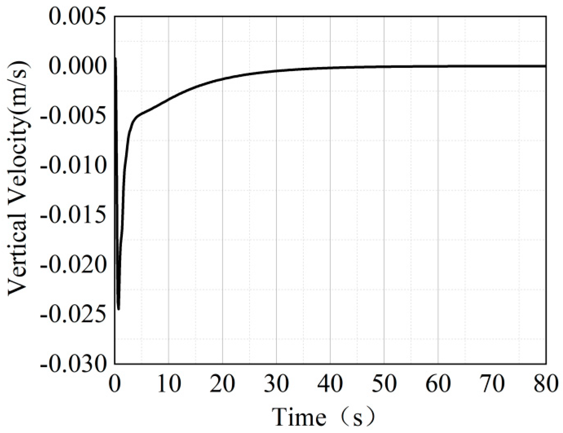
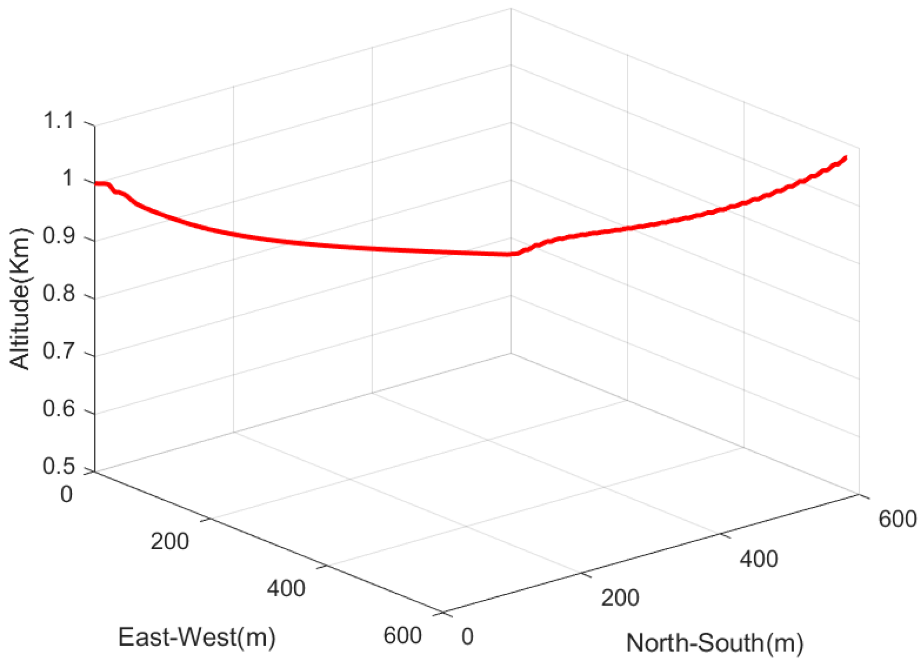
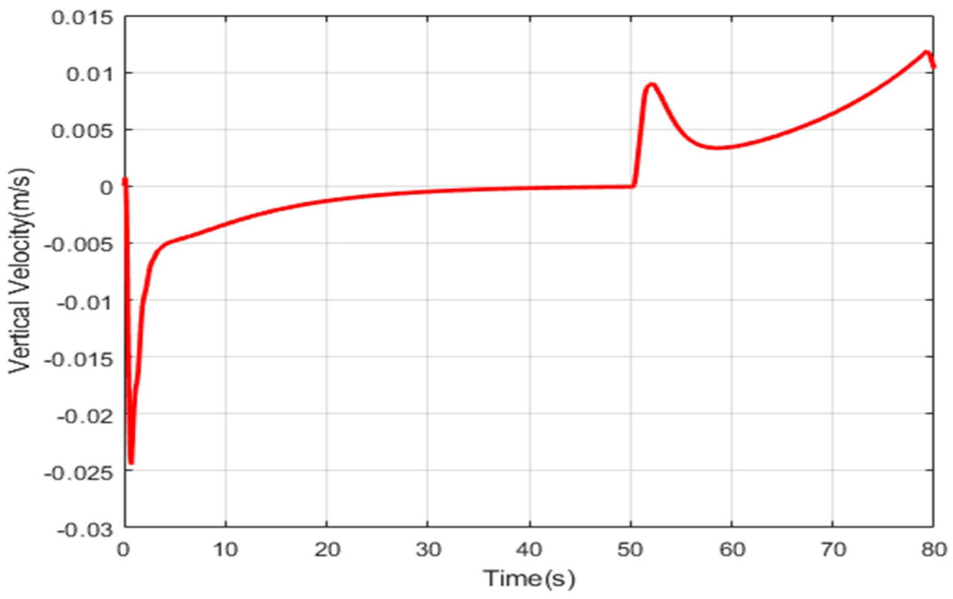
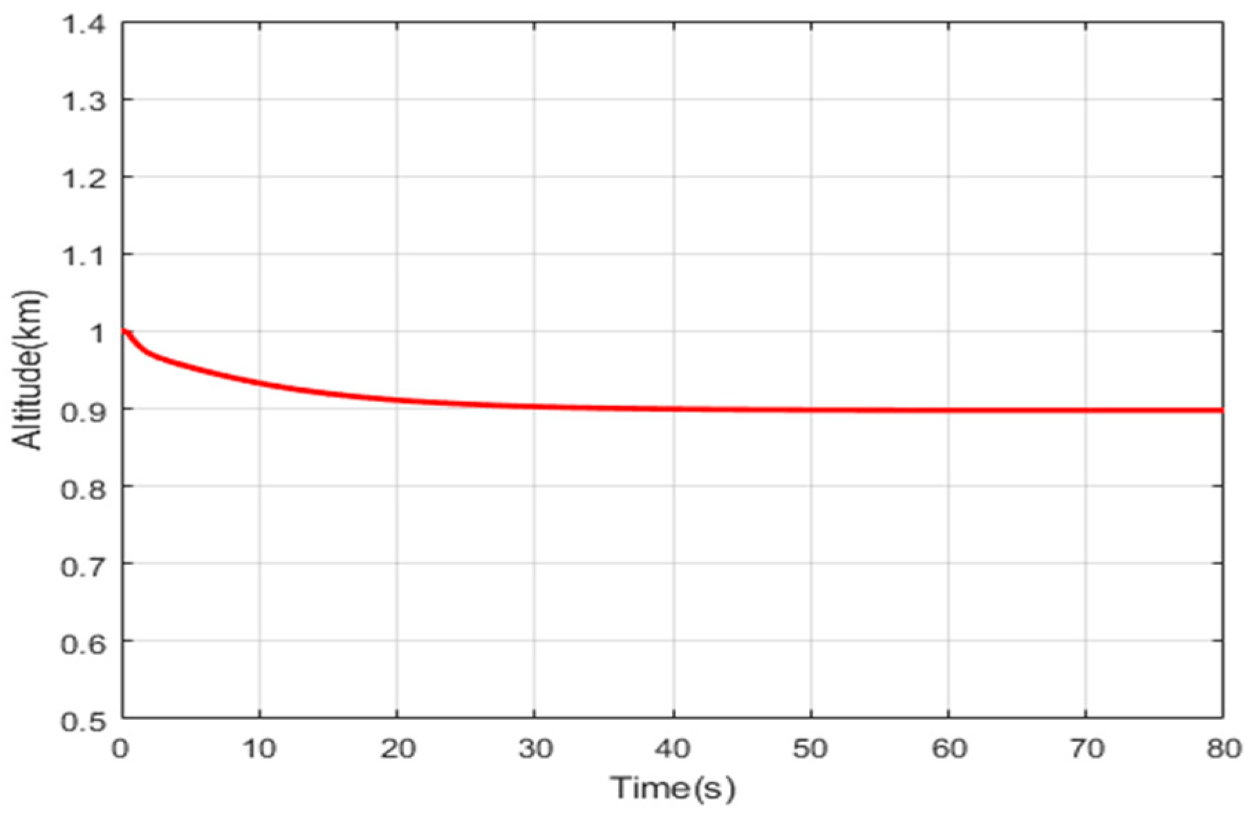
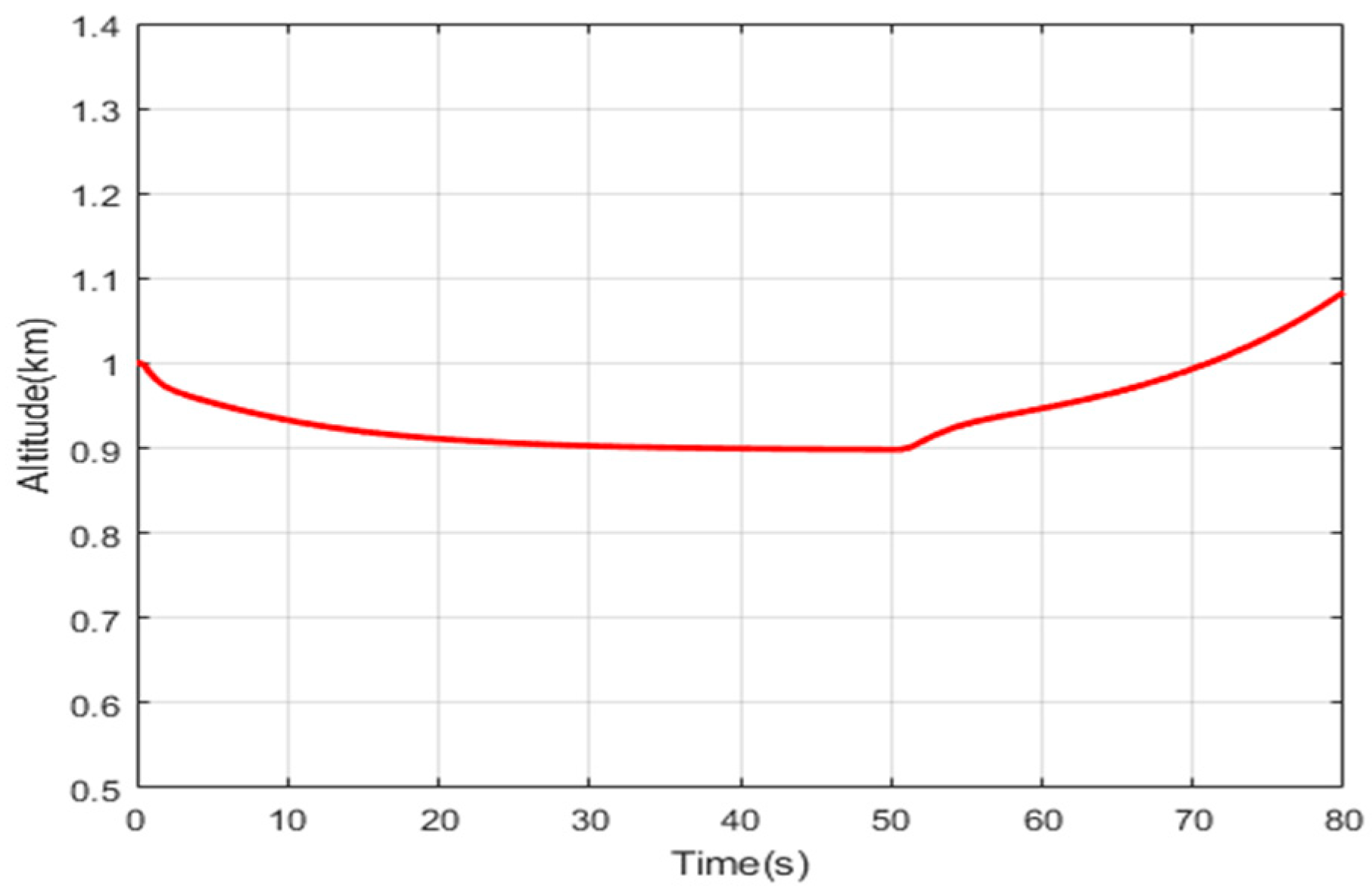
Figure 7. In the simulation performed in this study, the time of fault was consistent; however, to improve the readability of this article, the timeline is slightly adjusted in the displayed graphs. The linearized longitudinal state matrix of the “Beaver” aircraft was input into the flight control simulation model to collect the vertical velocity (Figure 8) and flight track of the aircraft under fault-free conditions (Figure 9) and the vertical velocity, altitude, and flight track of the aircraft under the fault condition (Figure 10, Figure 11 and Figure 12, respectively). In comparison, when the fault signal is added at 50 s, there will be slight fluctuations in the vertical velocity and altitude control of the aircraft. It can be seen from the flight track chart that the pitch angle of the aircraft increases slightly, and the altitude also increases.
Here, the detection and estimation of actuator element and gain faults are discussed to verify the proposed method. In addition, the robustness of the method to model uncertainties and disturbances is confirmed. We compare the performance of the proposed method with those of previously reported methods to verify its effectiveness.
The performance of the proposed method is evaluated via the simulation of actuator process and gain failures.
In the following simulation, we utilized  E = [ 1 1 0 0 ] T x ( 0 ) = [ 0 ,   0 ,   0 ,   0 ] T , and  ξ ( x , t ) = [ sin ( x 2 ) 0 sin ( x 2 ) 0 ] T . To transform the original model, the nonsingular transformation matrices   and   were calculated as follows:
= [ 0.7071 0.7071 0 0 0 0.7071 0.7071 0 0 0 0 0 1 0 0 0 0 0 1 0 0 0 0 0 1 ] = [ 0.7071   0.7071 0 0 0 0.7071 0.7071 0 0 0 0 0 1 0 0 0 0 0 1 0 0 0 0 0 1 ] . Then,  A 1 = [ 0.8345 4 . 7076 1 . 9559 0.1513 0 0 . 5162 4 . 7460 0 . 5847 0.1513 0 0 . 7804 0 . 4508 0 . 5519 0 0 0 . 7071 0 . 7071 0 . 1369 0 0 0 0 1.0093 0 0 ]   B = [ 5.1616 0 . 2495 5 . 1713 0.3134 0 . 1993 2 . 605 0 0 0 0 ] . In the simulation, the system disturbance is assumed to be bounded as  ψ      with  = 1.5  and  γ = 1 . By solving the LMI feasibility problems with the YALMIP toolbox, the following parameters were obtained:
α 1 = 1.6022 ,   μ = 0.0025 ,   P 1 = 0.0038 ,   P 2 = [ 0.0106 0.0483 0 ]
P 0 = [ 19.454 813.02 0 813.02 3.6131 0 0 0 3.6131 ] ,   F = [ 2620.7 1086.7 0.1082 0.0088 1542.5 21695 0.0064 0.0095 ]
L 0 = [ 42.0899 1.4076 15.8202 1.4011 2.4884 1.7884 1.1792 1.3974 0.3604 0.0645 0.9257 0 0 0.5047 0 0.9255 ]
Case 1: Actuator aging fatigue may cause incipient faults. The trend of incipient faults is slow. To simulate an incipient fault, it is preferable to choose the microvariation of the control input on the elevator drive motor as the simulation object. The system disturbance was selected as  ψ ( t ) = 0.02 × sin ( 300 t ) , corresponding to high-frequency interference. The incipient faults occurring in the input channel of the system  B l = D l  were considered. Figure 11, Figure 12 and Figure 13 show the detection of the fault  f a 1 = 0.03 × e 0.0667 t  with  t > 10   s  via the proposed method with  ν = 60 k = 5   and   δ = 0 . 01 .
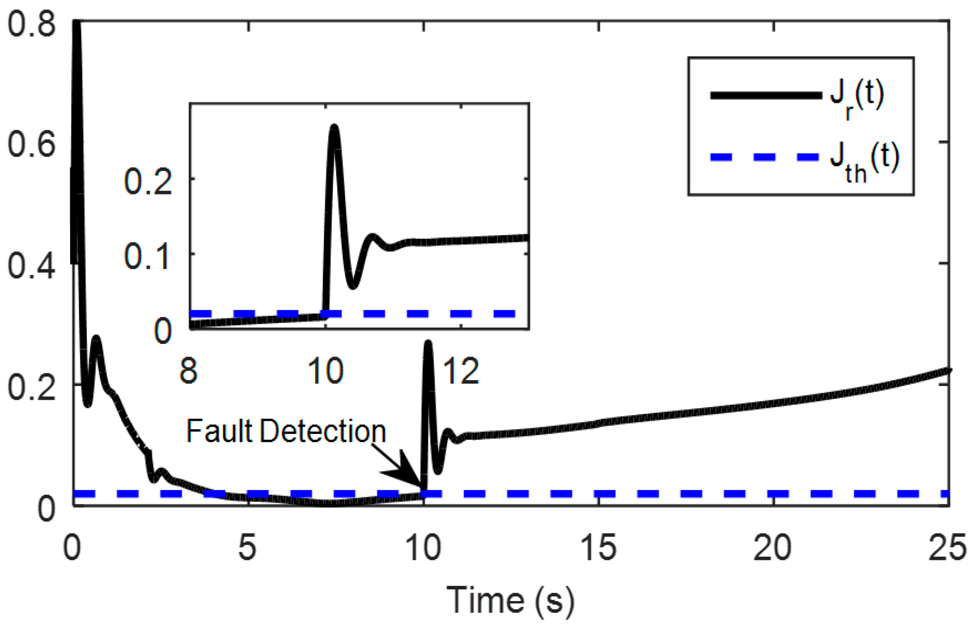
If there is no actuator fault in the system according to Remark 2, the evaluation function  J r  approaches zero.  J r  is close to zero before 10 s. When an actuator fault occurs, the evaluation function  J r  deviates from zero, as shown in Figure 13, Figure 14 and Figure 15 demonstrate that  J r  exceeds the threshold function  J t h  at approximately 10.15 s, which is the time at which the actuator fault occurs. Therefore, an actuator fault is detected and an alarm signal is generated. The convergence of the evaluation function shows that the proposed method is accurate for fault estimation of the actuator and that the adaptive reconstruction method is accurate for actual fault estimation.
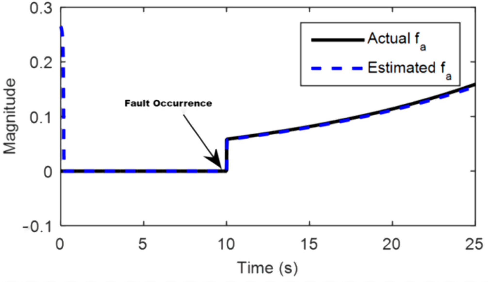
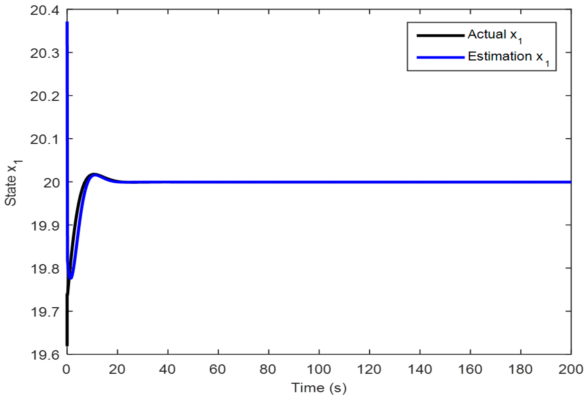
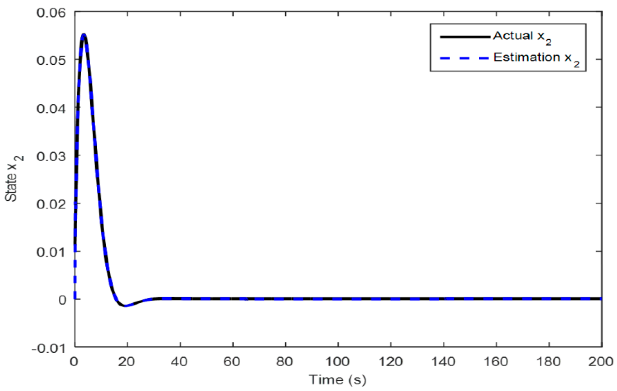
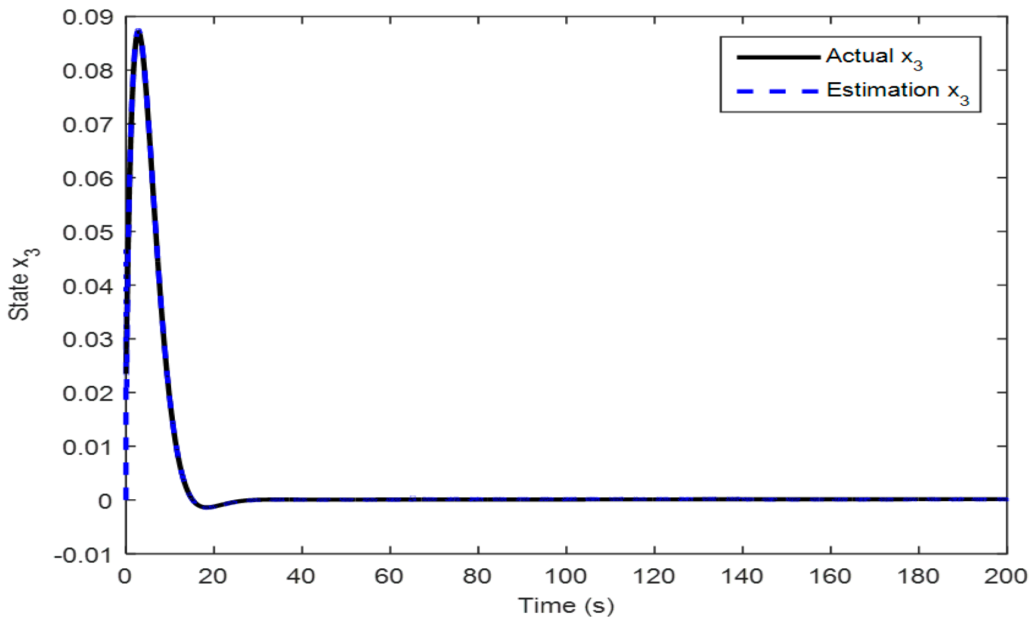
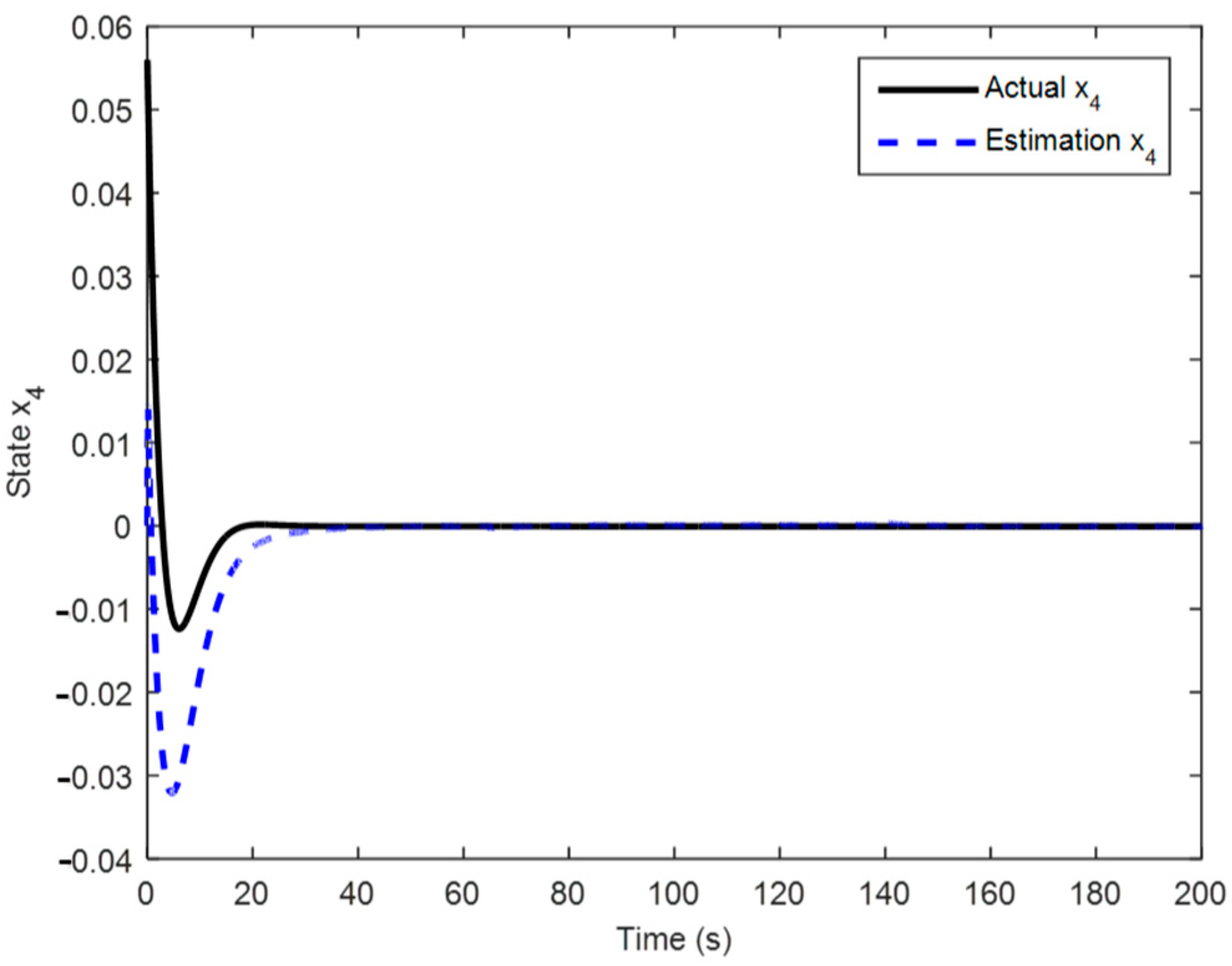
Figure 16, Figure 17, Figure 18 and Figure 19 present the trajectories of the state variables and their estimated values. These results demonstrate that the proposed method can accurately estimate the states. Further, the proposed method can avoid the influence of system interference and accurately reconstruct actuator faults. Minimizing the coefficient value of the proposed method improves the robustness of unknown signals and achieves the desired actuator fault reconstruction and state variable accuracy.
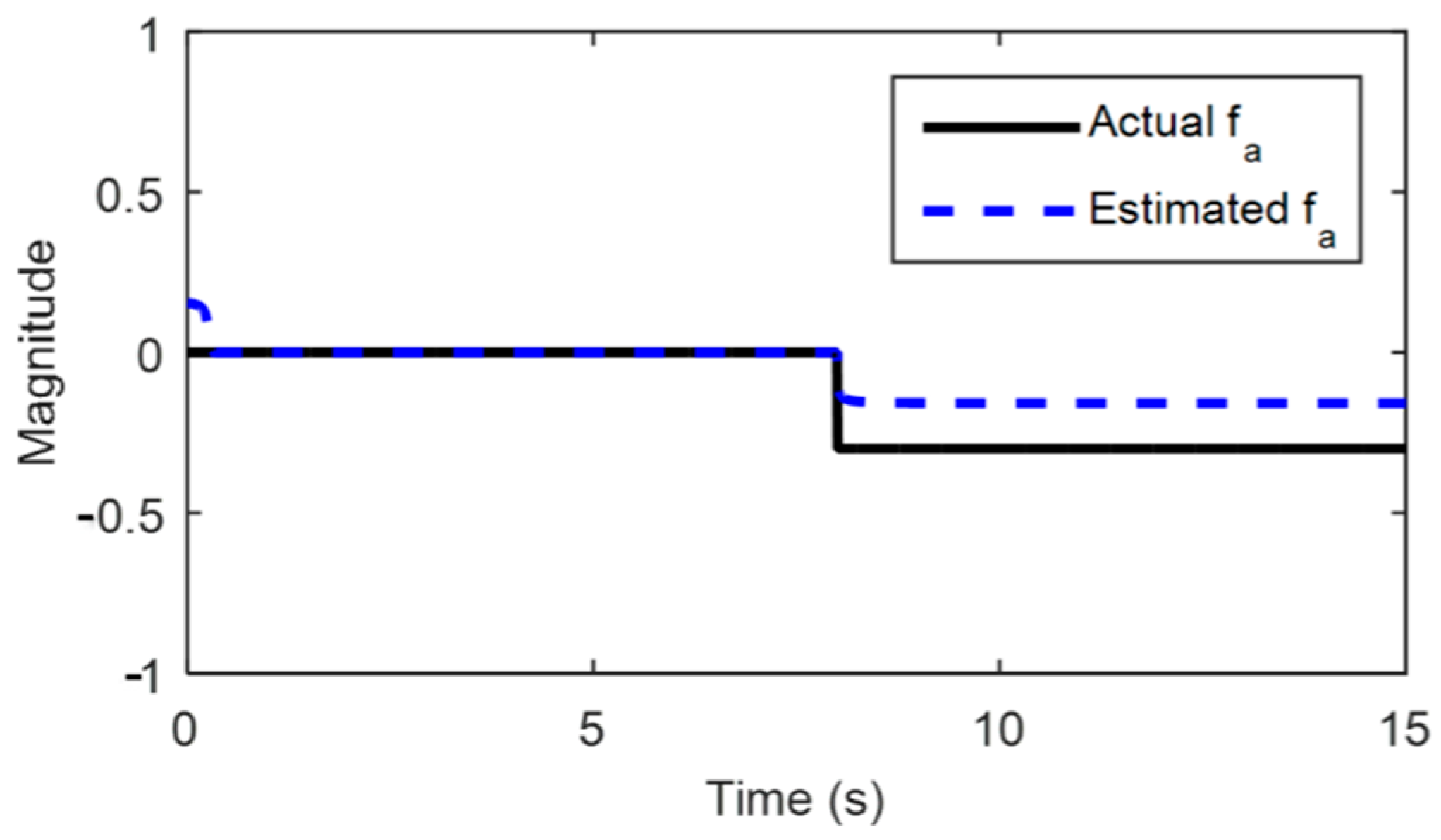
Case 2: In this case, an actuator gain fault (partial fault of the actuator control input) occurs. When the aircraft flight control system is unloaded, it is easily disturbed by the external airflow during flight, and the driving voltage cannot be accurately located on the reference voltage, which leads to small jumps and faults in the control input. This type of fault is minor, causing a very small number of faults, and is not easily detected. Partial faults and weak jumps of the control inputs were simulated in Simulation 2. The disturbance was selected as  ψ ( t ) = 0.02 × sin ( 300 t ) , corresponding to high-frequency interference. Consider the incipient faults occurring in the input channel of the system. Figure 20 and Figure 21 show the detection of the fault  f a 1 = 0.3 ε ( t 8 )  with  t 8   s  via the proposed method, with  ν = 42 k = 1.5   and   δ = 0 . 02 .
According to the second part of the theory, if there is no fault, the evaluation function  J r  approaches zero. In this case,  J r  is close to zero before 8 s. When an actuator fault occurs, the evaluation function  J r  deviates from zero, as shown in Figure 20. Figure 20 and Figure 21 demonstrate that  J r  exceeds the threshold function,  J t h , at 8.2 s. The convergence of the evaluation function shows that the proposed method can accurately estimate actuator faults, while the adaptive reconstruction method can accurately estimate actual faults.
The proposed method is verified using two fault examples, and the simulation results are compared with those obtained using the existing methods. For the incipient fault detection of closed-loop control systems, the total measurable fault information residual (ToMFIR) was proposed for the first time [39], which can collect comprehensive fault information in a closed-loop system. The ToMFIR consists of two parts: output residuals collected at the system output and controller residuals collected at the controller output. The output residuals represent the fault information for which the controller cannot compensate, and the compensated fault information exists in the controller residuals. In [39], an improved ToMFIR-based incipient fault detection and estimation method was proposed and applied to a high-speed railway vehicle suspension system. Although the improved ToMFIR method considered the system disturbance and utilized a more general framework, the incipient fault estimation method developed in this study removes the fault type limitation in [
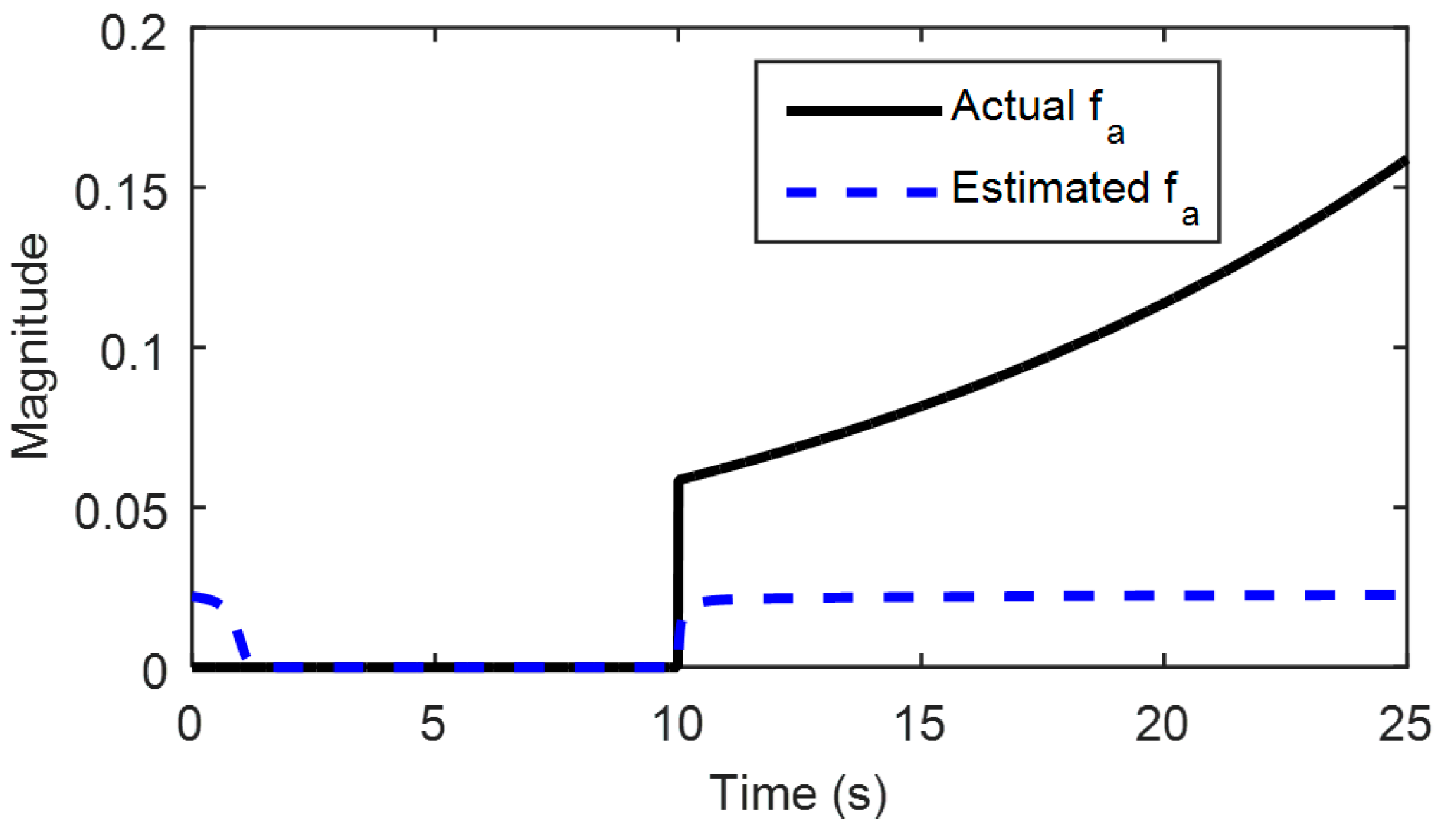
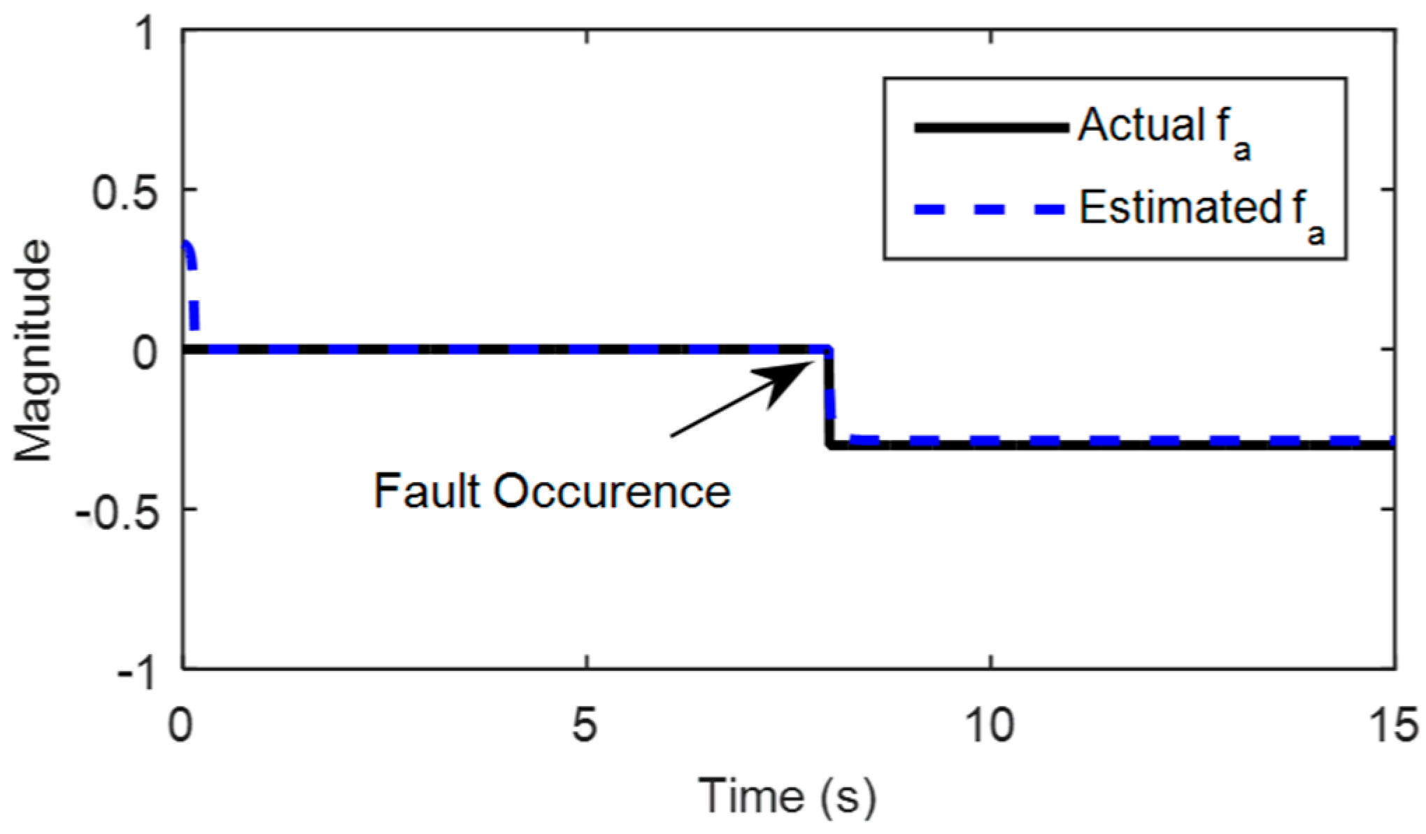
39]. The incipient fault estimation methods were used to estimate the faults of typical fixed-wing aircraft actuators, as shown in Figure 15 and Figure 22. The detection time, mean square error (MSE), and robustness of the methods to uncertainty were investigated. Table 5 summarizes the results of comparing the effectiveness of adaptive fault detection and fault reconstruction with that of the method reported in [39]. Comparisons of Figure 14 with Figure 15 and Figure 22 with Figure 23 reveal that the proposed method can match the actual actuator values more closely than the previous approach and thus has better estimation performance.

5. Conclusions

A robust fault detection and reconstruction method is proposed for a fixed-wing UAV model, which is represented by a nonlinear system with modeling and measurement uncertainties. Many previous studies have assumed that the state of the system can be measured and that the fault function is an additional term, which is different from the current approach. The method developed in this study focuses on fault detection and reconstruction of multiplicative actuator faults. Most component and actuator faults can be represented as multiplication faults, which the proposed method can detect and reconstruct. The developed method utilizes a Luenberger SMO and a robust adaptive strategy, which can simultaneously estimate the system state, generate residual signals, evaluate residual and reconstruct faults, and realize incipient fault detection and reconstruction. Finally, a De Havilland DHC-2 “Beaver” aircraft with Air Canada number 1244 was taken as an example to verify the effectiveness and robustness of the proposed method.
In the future, we will consider applying this method to more types of aircraft models and extend the fault detection and reconstruction method to the sensor.

Author Contributions

Conceptualization, L.W. and W.Z.; methodology, X.Z.; software, L.W.; validation, Q.D. and L.W.; formal analysis, L.W.; investigation, Z.L.; data curation, L.W. and K.W.; writing—original draft preparation, L.W.; writing—review and editing, X.Z.; visualization, Q.D.; supervision, W.Z.; project administration, Z.L.; funding acquisition, Z.L. All authors have read and agreed to the published version of the manuscript.

Funding

This research is supported in part by the National Natural Science Foundation Fund (No. 52072309), in part by the Key Research and Development Program of Shaanxi (No. 2019ZDLGY14-02-01), in part by the Shenzhen Fundamental Research Program (No. JCYJ20190806152203506), in part by the Aeronautical Science Foundation of China (No. ASFC-2018ZC53026), in part by the Stability Support Program for Higher Education Institutions in Shenzhen (No. 20200830220334001), and in part by the Beijing Institute of Spacecraft System Engineering (No. JSZL2020203B004).

Conflicts of Interest

The authors declare no conflict of interest.

Appendix A

Table A1. Aircraft parameter definitions.
ParameterMeaningUnits
β Sideslip anglerad
p Roll raterad s−1
γ Yaw raterad s−1
ϕ ˙ Back anglerad
ψ ˙ Yaw anglerad
θ Pitch anglerad
v True airspeedm s−1
α Attack anglerad
q Pitch raterad s−1
δ a Deflection of aileronsrad
δ r Deflection of rudderrad
δ e Deflection of elevatorrad
δ f Deflection of flapsrad
f a Actuator fault of aircraft
D l d ,   D l Known distribution matrix of actuator faults
Table A2. Model parameter definitions.
VariableDefinition
x l d [ β ,   ρ ,   γ ,   ϕ ,   ψ ] T
x l [ V ,   α ,   q ,   θ ] T
μ l d [ δ a ,   δ γ ]
μ l [ δ e ,   δ f ]
A l d [ Y ¯ β α ϕ + Y ¯ ρ Y ¯ γ 1 g cos θ ϕ / V ϕ 0 L ¯ β L ¯ ρ L ¯ γ 0 0 N ¯ β N ¯ ρ N ¯ γ 0 0 0 1 tan θ ϕ 0 0 0 1 1 / cos θ ϕ 0 0 ]
B l d [ 0 L δ α ¯ N δ α ¯ 0 0 Y δ γ ¯ L δ γ ¯ L δ γ ¯ 0 0 ] T
C l d 5D identity matrix
A l [ X V X α + g cos γ ϕ 0 g cos γ ϕ Z V Z α + g sin γ ϕ / V ϕ 1 g sin γ ϕ / V M ¯ V M ¯ α Z V M ¯ α M ¯ α ( Z α g sin γ ϕ / V ϕ ) M ¯ q + M ¯ α M ¯ α sin γ ϕ / V 0 0 1 0 ]
B l [ X δ d Z δ d M ¯ δ d M ¯ α Z δ d 0 X δ γ Z δ ρ M ¯ δ ρ M α Z δ ρ 0 ] T
C l 4D identity matrix

References

  1. Zhang, K.; Jiang, B.; Yan, X.G.; Shen, J.; He, X. Incipient fault detection based on robust threshold generators: A sliding mode interval estimation approach. IFAC-Pap. OnLine 2017, 50, 5067–5672. [Google Scholar] [CrossRef]
  2. Wang, D.; Shi, P.; Wang, W. Robust fault detection for continue-time switched delay systems: An linear matrix approach. IET Control Theory Appl. 2010, 4, 100–108. [Google Scholar] [CrossRef]
  3. Ke, Y.; Wang, K.; Chen, B.M. Design and Implementation of a hybrid UAV with model-based flight capabilities. IEEE/ASME Trans. Mechatron 2018, 23, 1114–1125. [Google Scholar] [CrossRef]
  4. Alwi, H.; Edwards, C. An adaptive sliding mode differentiator for actuator oscillatory failure case reconstruction. Automatica 2013, 49, 642–651. [Google Scholar] [CrossRef]
  5. Mao, Z.; Yan, X.G.; Jiang, B.; Chen, M. Adaptive fault-tolerant sliding-mode control for high-speed trains with actuator faults and uncertainties. IEEE Trans. Intell. Transp. Syst. 2020, 21, 2449–2460. [Google Scholar] [CrossRef]
  6. Jin, X.; Qin, J.; Shi, Y.; Zheng, W.X. Auxiliary fault tolerant control with actuator amplitude saturation and limited rate. IEEE Trans. Syst. Man Cybern. Syst. 2018, 48, 1816–1825. [Google Scholar] [CrossRef]
  7. Safaeipour, H.; Forouzanfar, M.; Casavola, A. A survey and classification of incipient fault diagnosis approaches. J. Process Control 2021, 97, 1–16. [Google Scholar] [CrossRef]
  8. Clark, R.N. Instrument fault detection. IEEE Trans. Aerosp. Electron. Syst. 1978, 14, 456–465. [Google Scholar] [CrossRef]
  9. Liu, J.; Yang, L.; Xu, M.; Zhang, Q.; Yan, R.; Chen, X. Model-based detection of soft faults using the smoothed residual for a control system. Meas. Sci. Technol. 2021, 32, 015107. [Google Scholar] [CrossRef]
  10. Chandra, K.P.B.; Chen, L.; Alwi, H.; Edwards, C. Development and evaluation of sliding mode schemes for the reconfigure benchmark problem. In Proceedings of the Conference on Control and Fault-Tolerant Systems, Barcelona, Spain, 7–9 September 2016; pp. 805–810. [Google Scholar]
  11. Zhang, J.; Swain, A.K.; Nguang, S.K. Detection and isolation of incipient sensor faults for a class of uncertain non-linear systems. IET Control Theory Appl. 2012, 6, 1870–1880. [Google Scholar] [CrossRef]
  12. Yan, K.; Chen, M.; Wu, Q.; Jiang, B. Extended state observer-based sliding mode fault-tolerant control for unmanned autonomous helicopter with wind gusts. IET Control Theory Appl. 2019, 13, 1454–1465. [Google Scholar] [CrossRef]
  13. Yan, X.G.; Edwards, C. Adaptive sliding-mode-observer-based fault reconstruction for nonlinear systems with parametric uncertainties. IEEE Trans. Ind. Electron. 2008, 55, 4029–4036. [Google Scholar]
  14. Zhang, J.; Swain, A.K.; Nguang, S.K. Robust sliding mode observer-based fault estimation for certain class of uncertain nonlinear systems. Asian J. Control 2015, 17, 1296–1309. [Google Scholar] [CrossRef]
  15. Chen, F.; Wang, Z.; Tao, G.; Jiang, B. Robust adaptive fault-tolerant control for hypersonic flight vehicles with multiple faults. J. Aerospace Eng. 2015, 28, 04014111. [Google Scholar] [CrossRef]
  16. Tan, C.P.; Edwards, C. An LMI approach for designing sliding mode observers for fault detection and isolation. In Proceedings of the European Control Conference, Pprto, Portugal, 4–7 September 2001; pp. 481–486. [Google Scholar]
  17. Nateghi, S.; Shtessel, Y.; Barbot, J.P.; Edwards, C. Cyber attack reconstruction of nonlinear systems via higher-order sliding-mode observer and sparse recovery algorithm. In Proceedings of the IEEE Conference on Decision and Control, Miami Beach, FL, USA, 17–19 December 2018; pp. 5963–5968. [Google Scholar]
  18. Shahriari-kahkeshi, M.; Sheikholeslam, F.; Askari, J. Adaptive fault detection and estimation scheme for a class of uncertain nonlinear systems. Nonlinear Dyn. 2015, 79, 2623–2637. [Google Scholar] [CrossRef]
  19. Zhang, X.; Polycarpou, M.M.; Parisini, T. A robust detection and isolation scheme for abrupt and incipient faults in nonlinear systems. IEEE Trans. Automat. Control 2002, 47, 576–593. [Google Scholar] [CrossRef]
  20. Liu, C.; Jiang, B.; Zhang, K. Incipient fault detection using an associated adaptive and sliding-mode observer for quadrotor helicopter attitude control systems. Circuits Syst. Signal Process. 2016, 35, 3555–3574. [Google Scholar] [CrossRef]
  21. Ding, B.; Fang, H. Fault prediction for nonlinear stochastic system with incipient faults based on particle filter and nonlinear regression. ISA Trans. 2017, 68, 327–334. [Google Scholar] [CrossRef]
  22. Zhang, Y.; Jiang, B. Bibliographical review on reconfigurable fault-tolerant control systems. Ann. Rev. Control 2008, 32, 229–252. [Google Scholar] [CrossRef]
  23. Quan, L.; Jiang, B.; Yang, P. Actuator fault diagnosis for flight control system based on sliding mode observer. In Proceedings of the 30th Chinese Control and Decision Conference, Shenyang, China, 9–11 June 2018; pp. 3243–3247. [Google Scholar]
  24. Hamayun, M.T.; Edwards, C.; Alwi, H. An output integral sliding mode FTC scheme using control allocation. Stud. Syst. Decis. Control 2016, 61, 81–101. [Google Scholar]
  25. Alwi, H.; Edwards, C.; Tan, C.P. Sliding mode estimation schemes for incipient sensor faults. Automatica 2009, 45, 1679–1685. [Google Scholar] [CrossRef]
  26. Chen, W.; Yeh, C.P.; Yang, H. ToMFIR-based fault detection approach in frequency domain. J. Syst. Eng. Electron. 2011, 22, 33–37. [Google Scholar] [CrossRef]
  27. Wu, Y.; Jiang, B.; Lu, N. Incipient winding fault detection and isolation for induction motors of high-speed trains. In Proceedings of the Prognostics and System Health Management Conference, Harbin, China, 9–12 July 2017; pp. 1–6. [Google Scholar]
  28. McLean, D. Automatic Flight Control Systems; Prentice Hall: Hertfordshire, UK, 1990. [Google Scholar]
  29. Martin, C.; Jay, T. State and input estimation for a class of uncertain systems. Automatica 1998, 34, 757–764. [Google Scholar]
  30. Ben Brahim, A.; Dhahri, S.; Ben Hmida, F.; Sellami, A. Simultaneous actuator and sensor faults reconstruction based on robust sliding mode observer for a class of nonlinear systems. Asian J. Control 2017, 19, 362–371. [Google Scholar] [CrossRef]
  31. Zhou, M.; Wang, Z.; Shen, Y. Fault detection and isolation method based on H−/H∞ unknown input observer design in finite frequency domain. Asian J. Control 2017, 19, 1777–1790. [Google Scholar] [CrossRef]
  32. Yu, L.; Xu, J.M.; Han, Q.L. Optimal guaranteed cost control of singular systems with delayed state and parameter uncertainties. In Proceedings of the American Control Conference, Boston, MA, USA, 30 June–2 July 2004; pp. 4811–4816. [Google Scholar]
  33. Edwards, C.; Tan, C.P. A comparison of sliding mode and unknown input observers for fault reconstruction. Euro J. Control 2006, 12, 245–260. [Google Scholar] [CrossRef]
  34. Nagesh, I.; Edwards, C.; Alwi, H. Comparison between unit vector and super-twisting sliding mode FDI design for actuator faults. In Proceedings of the Conference on Control and Fault-Tolerant Systems, Nice, France, 9–11 October 2013; pp. 146–151. [Google Scholar]
  35. Patel, N.; Edwards, C.; Spurgeon, S.K. An analysis of two nonlinear observers in the presence of noise. In Proceedings of the American Control Conference, Seattle, WA, USA, 11–13 June 2008; pp. 242–247. [Google Scholar]
  36. Zhao, K.; Li, P.; Zhang, C.; Li, X.; He, J.; Lin, Y. Sliding mode observer-based current sensor fault reconstruction and unknown load disturbance estimation for PMSM driven system. Sensors 2017, 17, 2833. [Google Scholar] [CrossRef]
  37. Fang, P.; Chen, W.; Zhang, G. Flight Dynamics of Aeronautical Vehicles; Beijing University of Aeronautics and Astronautics Press: Beijing, China, 2005; pp. 40–64. [Google Scholar]
  38. Rauw, M. A Simulink Environment for Flight Dynamics and Control Analysis Application to the DHC-2 ‘Beaver’. Ph.D. Thesis, Delft University of Technology, Delft, The Netherlands, 1993; pp. 152–180. [Google Scholar]
  39. Wu, Y.; Jiang, B.; Lu, N.; Yang, H.; Zhou, Y. Multiple incipient sensor faults diagnosis with application to high-speed railway traction devices. ISA Trans. 2017, 67, 183–192. [Google Scholar] [CrossRef] [PubMed]
Figure 1. Schematic diagram of aircraft parameters.
Aerospace 10 00422 g001
Figure 2. Block diagram of the proposed robust fault diagnosis method.
Aerospace 10 00422 g002
Figure 3. The model of De Havilland DHC-2 “Beaver” aircraft.
Aerospace 10 00422 g003
Figure 4. Basic control–response relationships for “Beaver”.
Aerospace 10 00422 g004
Figure 5. Fault injection flow chart.
Aerospace 10 00422 g005
Figure 6. Flight control simulation model.
Aerospace 10 00422 g006
Figure 7. Fault signal in case 1.
Aerospace 10 00422 g007
Figure 8. Vertical velocity under fault-free conditions.
Aerospace 10 00422 g008
Figure 9. Altitude under fault-free conditions.
Aerospace 10 00422 g009
Figure 10. Flight track under fault-free conditions.
Aerospace 10 00422 g010
Figure 11. Vertical velocity under fault condition.
Aerospace 10 00422 g011
Figure 12. Altitude under fault condition.
Aerospace 10 00422 g012
Figure 13. Flight track under fault conditions.
Aerospace 10 00422 g013
Figure 14. Evaluation function and threshold.
Aerospace 10 00422 g014
Figure 15. Actual fault and its estimation with DAF.
Aerospace 10 00422 g015
Figure 16. Actual fault and its estimation with ToMFIR.
Aerospace 10 00422 g016
Figure 17. State x1 and its estimation.
Aerospace 10 00422 g017
Figure 18. State x2 and its estimation.
Aerospace 10 00422 g018
Figure 19. State x3 and its estimation.
Aerospace 10 00422 g019
Figure 20. State x4 and its estimation.
Aerospace 10 00422 g020
Figure 21. Evaluation function and threshold.
Aerospace 10 00422 g021
Figure 22. Actual fault and its estimation with DAF.
Aerospace 10 00422 g022
Figure 23. Actual fault and its estimation with ToMFIR.
Aerospace 10 00422 g023
Table 1. Parameter definitions.
ParameterMeaning
FMMeasurement reference frame
FSStability reference frame
FRSpecial body-fixed reference frame for the “Beaver”
FWFlight-path reference frame
FVVehicle-carried vertical reference frame
FxTotal external force along XB
FyTotal external force along YB
FzTotal external force along ZB
Table 2. Actuator fault diagnosis steps.
StepDescription
Step 1Set the matching conditions of the system and make relevant assumptions
Step 2Establish the system model, and make it meet certain conditions
Step 3Calculate the nonsingular transformation matrix to decouple the system model
Step 4Design the observer according to the transformed form of the system
Step 5Based on the establishment of the error equation of state estimation, the evaluation function and threshold are obtained according to the theoretical knowledge in Chapter 3
Step 6Calculate relevant parameters according to the LMI algorithm
Step 7Use the calculated relevant parameters to substitute them into the observer algorithm for actuator fault diagnosis
Table 3. Actuator fault reconstruction steps.
StepsDescription
Step 1Set system matching conditions and make relevant assumptions based on fault detection
Step 2Calculate the tensor matrix and transform the output matrix in the system model
Step 3Calculate the nonsingular transformation matrix to further decouple the system model
Step 4Design the observer algorithm according to the transformed model
Step 5The idea of solving the problem is converted into LMI form, and the observer parameters are calculated by the LMI algorithm
Step 6Reconstruct actuator faults through adaptive fault reconstruction
Table 4. “Beaver” parameter definitions.
ParameterValue
Wing span b14.63 m
Wing area S23.23 m2
Mean aerodynamic chord c1.5875 m
Wing dihedral
Wing profileNACA 64 A 416
Fuselage length9.22 m
Max. take-off weight2280 kg
Empty weight1497 kg
Max. power450 Hp at n = 2300 RPM, pz = 26″Hg
Table 5. Performances of the adaptive fault detection and reconstruction method and ToMFIR [26,39].
CriteriaAdaptive Fault Detection and Reconstruction MethodToMFIR
Detection time of case 110.15 s-
Detection time of case 28.2 s-
MSE of case 15.6921 × 10−44.1245
MSE of case 22.9911 × 10−43.5828
Disclaimer/Publisher’s Note: The statements, opinions and data contained in all publications are solely those of the individual author(s) and contributor(s) and not of MDPI and/or the editor(s). MDPI and/or the editor(s) disclaim responsibility for any injury to people or property resulting from any ideas, methods, instructions or products referred to in the content.

