
Aerodynamic Optimization Design of Supersonic Wing Based on Discrete Adjoint
1
School of Aeronautics, Northwestern Polytechnical University, Xi’an 710072, China
2
School of Aeronautics, Xi’an Jiaotong University, Xi’an 710049, China
3
AVIC the First Aircraft Institute, Xi’an 710089, China
*
Author to whom correspondence should be addressed.
Aerospace 2023, 10(5), 420; https://doi.org/10.3390/aerospace10050420
Submission received: 25 February 2023
/
Revised: 24 April 2023
/
Accepted: 25 April 2023
/
Published: 29 April 2023
(This article belongs to the Special Issue Adjoint Method for Aerodynamic Design and Other Applications in CFD)
Abstract
:Reducing fuel consumption and improving the economy by effectively reducing cruising drag is the main objective of the aerodynamic design of supersonic civil aircraft. In this paper, the aerodynamic optimization design system based on the Reynolds-Averaged Navier–Stokes (RANS) equation and discrete adjoint theory is applied to supersonic wing design. Based on this system, a single-point optimization design study of aerodynamic drag reduction in cruise conditions was carried out for two typical supersonic wing layouts, subsonic leading edge and supersonic leading edge, and the drag reduction reached 3.78% and 4.53%, respectively. The aerodynamic design characteristics of different types of supersonic wings were explored from the perspectives of wing load, twist angle distribution, pressure distribution, airfoil shape characteristics, and flow field characteristics. The optimization results show that the drag reduction of the subsonic leading edge configuration is dominated by the induced drag, while the optimizer mainly focuses on reducing the shock wave drag for the supersonic leading edge configuration. By comparing the sensitivity analysis of lift and drag coefficients to airfoil deformation with the optimization results, the optimized dominant directions of two types of supersonic wings are qualitatively analyzed. The derivatives obtained from discrete adjoint equations are useful to elaborate the design tendency and the reason for the trade-off generation of supersonic wings under specific layouts and engineering constraints, which provides a reference for the design of supersonic wings in the future.
1. Introduction
With the rapid development of the air transport industry, transoceanic flights have greatly promoted political, economic, and cultural exchanges among countries around the world. Although high-subsonic transport aircraft have achieved great success, long flight times have seriously reduced comfort and travel efficiency for long distance flights [1]. In transoceanic flight, supersonic civil aircraft can save about half of the time compared with non-supersonic, which has its own unique advantages in the market competition. Therefore, supersonic civil aircraft has become a key area of focus for future civil aircraft development. The first-generation supersonic civil aircraft, such as “Concorde” and Tu-144 [2,3], verified the technical feasibility of supersonic transport (SST). However, for complicated reasons, no new-generation supersonic civil aircraft has been put into operation so far, but research on the new-generation SST in the United States, Japan, and Europe has never stopped. For example, the United States has proposed the Supersonic Cruise Research (SCR) program and the High Speed Civil Transport (HSCT) program [4] to establish a feasible supersonic cruise technology and to conduct technical basic research on eco-friendly supersonic civil aircraft. Europe has formulated a High Speed Aircraft (HISAC) research program [5], and Japan has launched a National Experimental Supersonic Transport (NEXST) program [6]. The increasing requirements of various countries for reducing fuel consumption, sonic boom, and noise have created huge technical challenges and high cost issues for the research of large supersonic civil aircraft. Therefore, the National Aeronautics and Space Administration (NASA) has proposed the research plan for the next three generations of supersonic civil aircraft [7], which will shift the focus of recent research to medium and small supersonic business jets with a cruising Mach number of 1.6–1.8 or even lower speeds. By promoting the development of related technologies to gradually achieve the goal of designing large supersonic civil aircraft, the United States has made some efforts to develop three types of supersonic business jets, Aerion AS2, Spike S-512, and NASA X-59, although Aerion AS2 was canceled in 2021.
The aerodynamic shape determines the aerodynamic performance of an aircraft to a large extent. Reducing the overall drag mainly depends on the design of the aerodynamic shape of the aircraft. Therefore, for supersonic civil aircraft, effectively reducing the overall drag has become the main goal of aerodynamic design. Aerodynamic shape optimization design uses the numerical optimization algorithm and its auxiliary technologies, combined with Computational Fluid Dynamics (CFD) technology to implement the automatic design of aerodynamic shape and pursue the optimal aerodynamic performance. At present, the aerodynamic shape optimization design has been widely recognized and was successfully conducted in multiple engineering applications [8,9,10,11].
Supersonic civil aircraft are streamlined to reduce the drag. The finely designed wing usually has the best combination of bend and twist, which makes the design space for supersonic wings more complicated, and there are interference problems between the wing and the fuselage. Based on the above characteristics, three-dimensional integrated fine design is necessary for the aerodynamic shape optimization design of supersonic civil aircraft, so the related optimization problems involve large-scale design variables and constraints.
The optimization algorithm used in the aerodynamic shape optimization design controls the entire design process and determines the direction of the optimization design. According to whether gradient information needs to be solved, optimization algorithms can be divided into gradient-free algorithms and gradient-based algorithms. Lyu et al. [12] studied the growth law of the number of calls to the objective function by different optimization algorithms as the number of design variables increased. The results show that as the number of design variables increases, the number of calls to the objective function by the gradient-based optimization algorithm basically increases linearly, while the gradient-free optimization algorithm increases by the second power or higher. When solving the gradient based on the discrete adjoint approach, the calculation amount is almost not dependent on the number of design variables, but only related to the number of objective functions or constraints, so it can quickly and accurately handle aerodynamic optimization design problems involving large-scale design variables and constraints. Therefore, for the large-scale design variables in the aerodynamic shape optimization design of supersonic civil aircraft, the gradient-based optimization method based on discrete adjoint can take into account both high efficiency and reliability [13,14].
For the aerodynamic shape optimization of SST, relevant results have been obtained based on gradient and heuristic methods. Using the optimization method combining the simplex method and the genetic algorithm, Chan [15] carried out a comprehensive optimization design research study on low sonic boom and low drag for SST aircraft. By constructing a surrogate model of aerodynamic force and sonic boom response, Choi et al. [16] conducted a low-boom and low-drag comprehensive optimization design for supersonic business jets. Kirz [17] carried out multi-objective optimization of coupling aerodynamic and sonic boom for the JAXA S4 supersonic airliner based on the surrogate model approach.
Compared with heuristic methods, gradient-based optimization design has been more widely studied and applied due to its high efficiency. Kiyici and Aradag [18] carried out the aerodynamic optimization design for supersonic business jets using the high-fidelity combined CFD solver and optimizer SU2 for numerical simulation calculations. Based on the gradient-based optimization algorithm, the supersonic drag was reduced by 14% and the lift-to-drag ratio was increased by 10%. The high-fidelity multidisciplinary optimization framework MACH based on the RANS equation is currently an advanced and relatively mature discrete-adjoint optimization design system in this field. It has obvious advantages such as calculation efficiency in dealing with the optimization design with massive design variables. Based on the MACH optimization framework, Li et al. [19] carried out research on the aerodynamic optimization design of supersonic aircraft for reducing drag. Using a gradient-based aerodynamic optimization design system, the optimization result effectively suppressed the shock wave region of the wing, and the shock wave intensity was significantly reduced. The drag reduction of the whole configuration reached 5.7%. Liu et al. [20] improved the aerodynamic optimization framework. The gradient of the sonic boom value was obtained using the finite difference method and combined with the gradient of the aerodynamic objective function with respect to the design variables. They established an aerodynamic optimization design method considering the sonic boom characteristics, and carried out an optimization design study on the wing-body configuration of a supersonic business jet. Liu et al. [21] proposed an adjoint optimization method for coupling aerodynamic and near-field sonic boom characteristics. Aiming at the supersonic airliner standard model, a comparative study was carried out under three strategies, namely, low-drag optimization, near-field low sonic boom reverse design, and adjoint optimization for coupling aerodynamic and near-field sonic boom characteristics.
The design of an SST aircraft needs to consider the compromise between high-speed performance and low-speed stability, and numerical optimization provides the opportunity to obtain the best high-speed performance while maintaining low-speed stability. Seraj and Martins [22] used the component-based geometric parameterization method to optimize the aerodynamic shape based on the RANS equation. The drag minimization study for the supersonic cruise condition was performed separately with and without the subsonic pitch stability constraint, and the supersonic drag penalty associated with the subsonic stability constraint was quantified. This provides a reference for the compromise design between supersonic performance and subsonic stability. Based on the MACH framework, Bons et al. [23] and others carried out a multidisciplinary optimization design for the AS2 configuration of Aerion Company. They explored the compromise design space between aerodynamics and structure and reduced the passive load of the wing through static aeroelastic tailoring.
According to the published design scheme of SST [24,25], the wings of supersonic civil aircraft mainly have two layout forms: the subsonic leading edge and supersonic leading edge. Their different flow physical characteristics make the two types of supersonic wings have different aerodynamic drag reduction principles. Understanding the aerodynamic design principles of different types of supersonic wings is of great significance to the development of supersonic civil aircraft. However, there is currently limited research on the differences in the aerodynamic optimization design of two typical supersonic wing layouts. Meanwhile, there is a lack of work on the use of gradient information fields to analyze the optimal design direction of supersonic wings and the effective trade-off between different aerodynamic drags, which is the key to guiding the design of supersonic wings in the future. Therefore, this paper takes the subsonic leading edge and supersonic leading edge as the research objects, and the aerodynamic optimization design system based on discrete adjoint is adopted to carry out the single point optimization design for reducing aerodynamic drag at cruise conditions. The principle of aerodynamic drag reduction is explored from the perspectives of wing load, twist distribution, pressure distribution, airfoil shape characteristics, and flow field characteristics. The similarities and differences between the aerodynamic design principles of two different types of supersonic wings are preliminarily revealed. The sensitivity analysis results of the lift and drag coefficient to the wing deformation are obtained by using the gradient information. Combined with the optimization results, the optimization dominant direction of the supersonic aircraft and the effective trade-off between lift and drag, and wing profile deformation and constraints during the optimization process are analyzed qualitatively.
This paper is structured as follows. Section 2 introduces the numerical simulation method and discrete adjoint method. Section 3 describes the establishment of the optimization framework. The optimization results of two types of supersonic configuration are, respectively, shown in Section 4 and Section 5. Finally, we summarize our work in Section 6.
2. Numerical Simulation Method and Discrete Adjoint Equation
2.1. Numerical Simulation Method
Accurate numerical simulation of flow field is the basis of aerodynamic optimization design. This paper uses RANS solver ADflow [26] for structured mesh and overset mesh, which can accurately predict aerodynamic force and perform gradient calculation based on the discrete adjoint approach.
The numerical simulation uses the three-dimensional compressible RANS equation as the governing equation of the flow field, and its integral form is defined as Equation (1).
where V is the volume boundary of the control volume, is the conserved variable of the flow field, and are the inviscid flux and the viscous flux, respectively. The Spalart–Allmaras (SA) one-equation turbulence model is used in this work [27].
The spatial discretization adopts the Jameson–Schmidt–Turkel (JST) second-order central difference scheme based on the finite volume method [28]. ADflow supports several explicit and implicit pseudo-time-advancing methods. The explicit method includes the five-order Runge–Kutta (RK) method [28]; the implicit method includes the Diagonalized-Diagonally-Dominant Alternating Direct Implicit (D3ADI) method [29], Newton–Krylov method (NK) [30,31], Approximate Newton–Krylov method (ANK) [32] and LU-SGS method [33]. The ADflow solver can implement the efficient solution and deep convergence of the RANS equation. The specific solution process is as follows. Firstly, the RK, D3ADI, or ANK algorithm is used to solve a better initial solution . When the flow field residual reaches a certain convergence standard, the solver switches to the NK algorithm, which can make the flow field solution converge quickly and deeply. When solving large-scale coefficient linear systems, ADflow uses the Generalized Minimal Residual (GMRES) method of the open source Petsc library.
2.2. Validation of Simulation Method
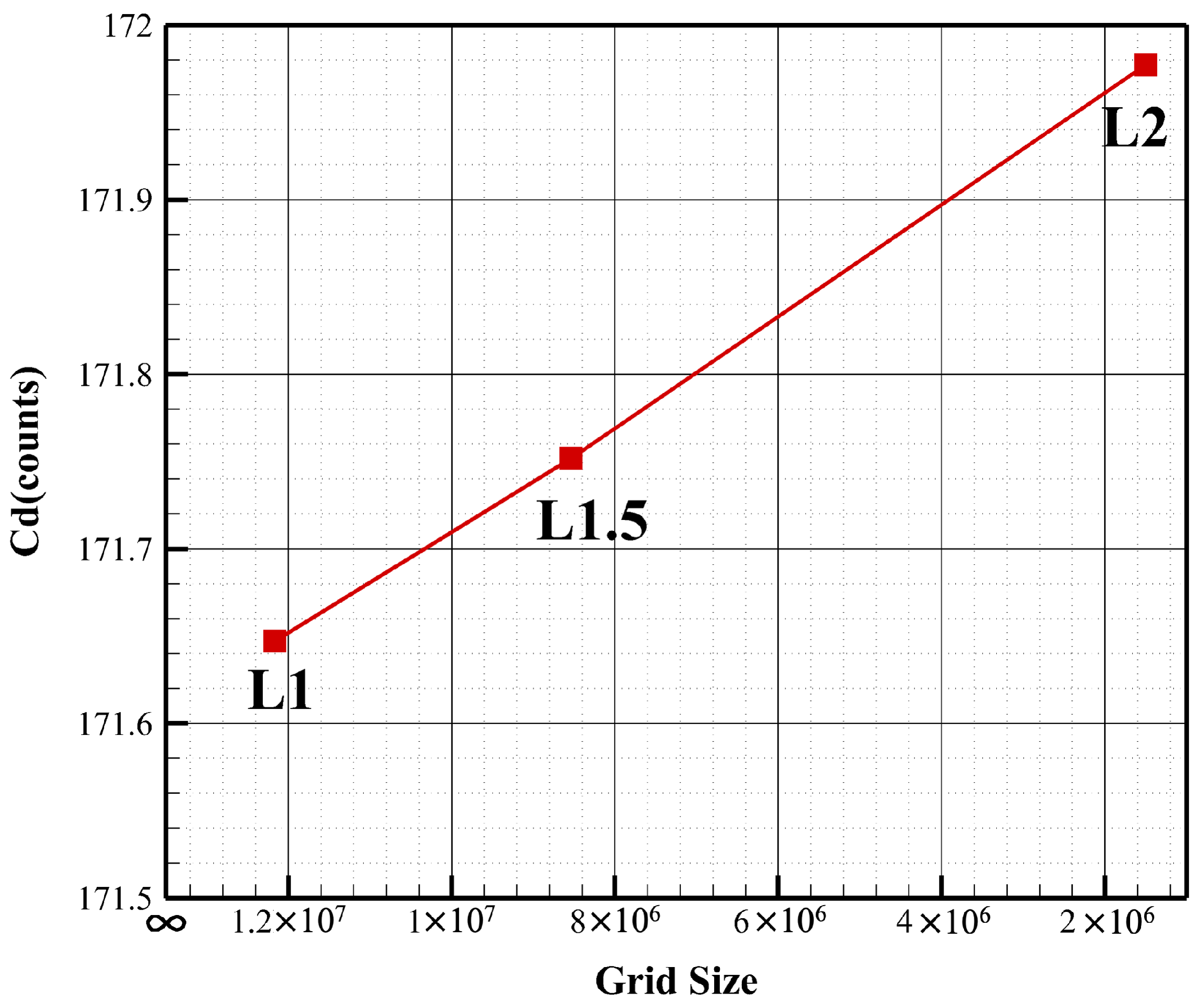
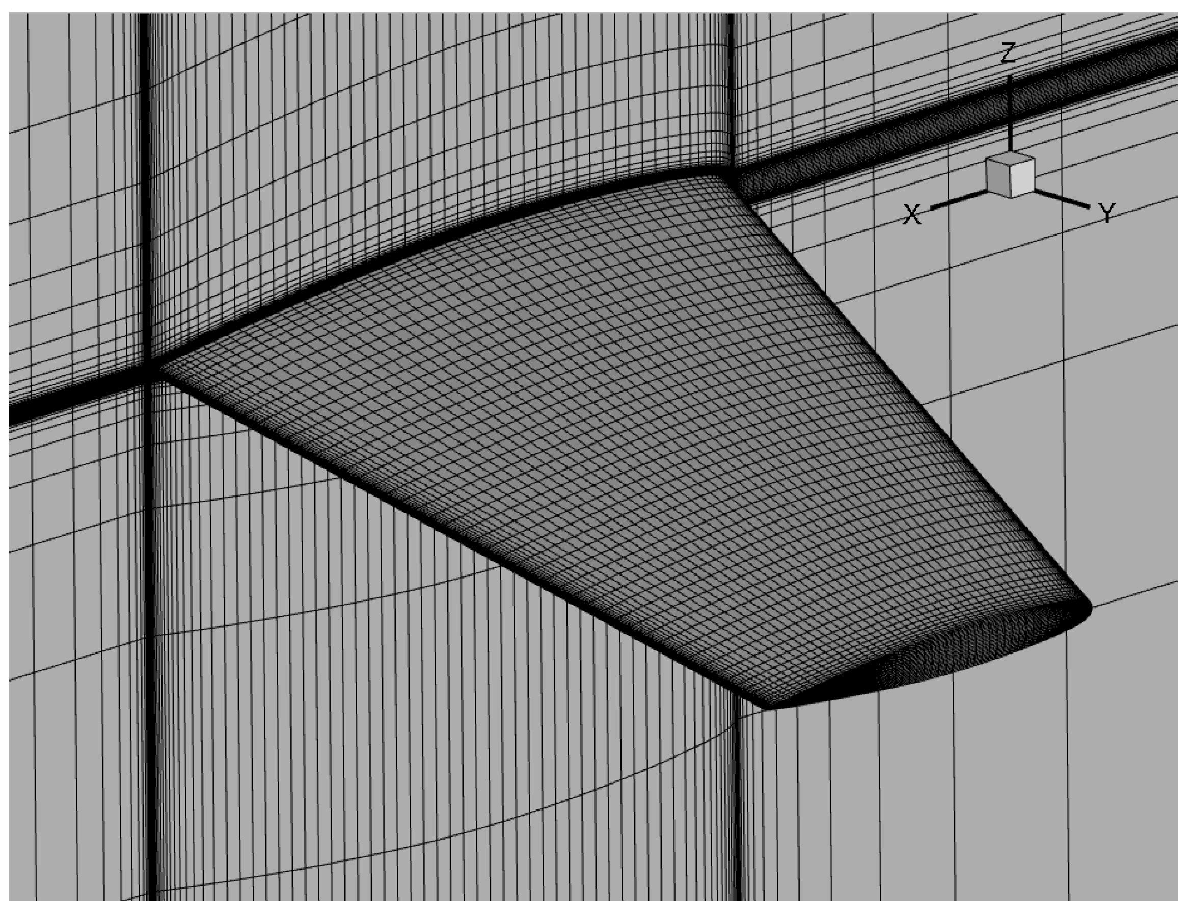
We validate the solver accuracy using the ONERA-M6 airfoil. The calculation condition is , , and angle of attack is . The reason for choosing this condition is because there are detailed experimental data [34]. Using commercial software ICEM to divide multi-block structure mesh. For the solver used in this paper, we have conducted a mesh convergency study using three levels of the grid, named coarse (L2, 1.5 million), medium (L1.5, 8 million), and fine (L1, 12 million). The numerical simulation of the flow field is carried out on the M6 wing, and the results are shown in Figure 1. It can be seen from the figure that the drag deviation calculated by the three levels of grids does not exceed 0.5 counts, the L2 grid with a grid volume of 1.5 million can perform a good calculation and evaluation of the drag of the M6 wing, and the grid amount is relatively small. The L2 grid is shown in Figure 2.
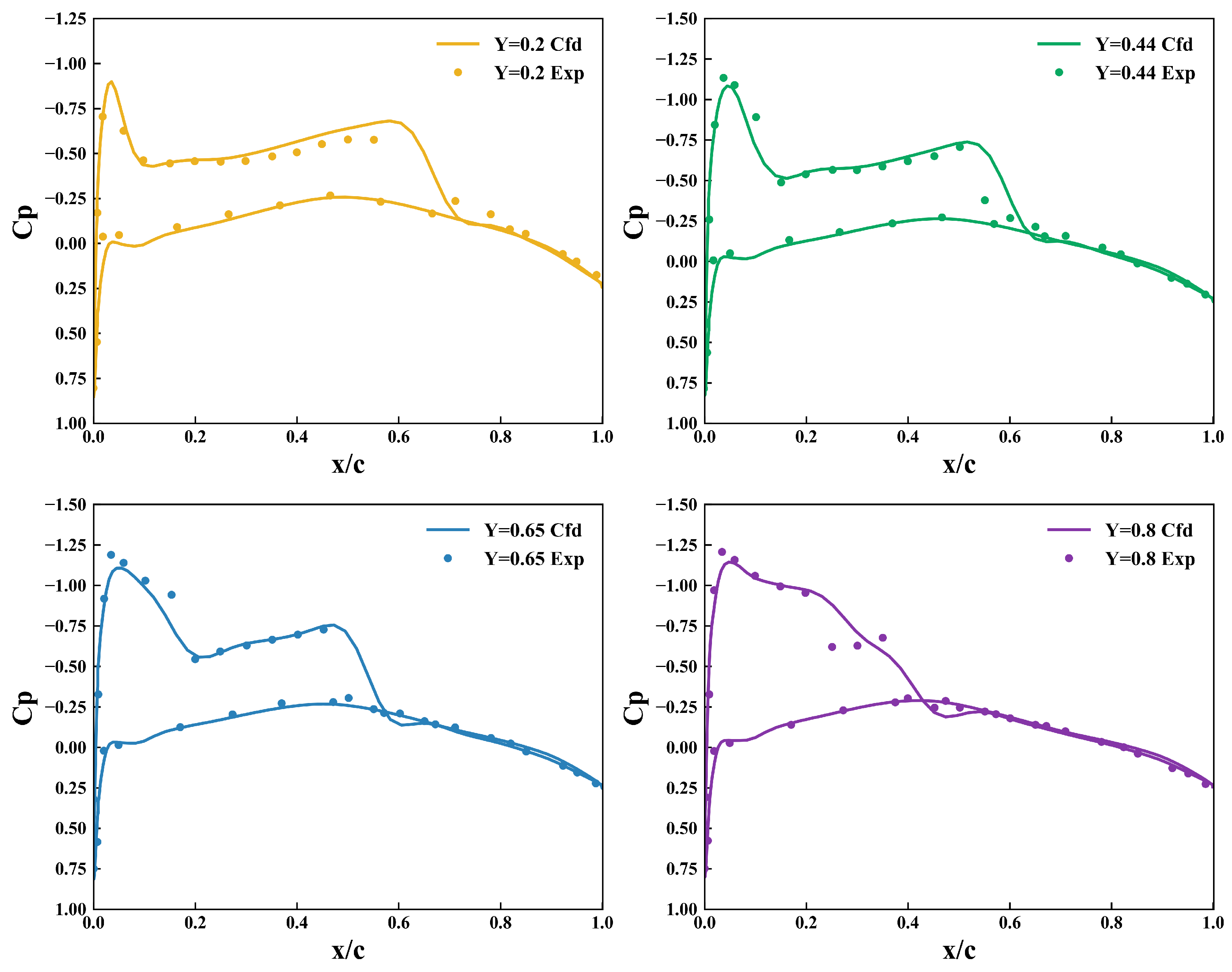
Four sections of 20%, 44%, 65%, and 80% semi-span were taken along the span of the wing. The comparison between the calculation results of the solver and the experimental data is shown in Figure 3. The circular data points in the figure are the experimental data, and the solid line is the calculated cross-sectional pressure distribution. It can be seen that the calculation results and the experimental data are in good agreement in each spanwise section of the wing, indicating that the CFD solver meets the accuracy requirements of the optimal design.
2.3. Discrete Adjoint Equation
In the gradient-based optimization design, it is a key step to efficiently and accurately obtain the derivative of the objective function with respect to the design variables. Commonly used gradient solution methods include the finite difference method, complex variable difference method, and adjoint equation method. The calculation cost of the finite difference method and the complex variable difference method is not acceptable when the design variables increase, so they are not suitable for aerodynamic optimization design problems with high-dimensional characteristics. The efficiency of solving the gradient with the adjoint equation method is almost not affected by the number of design variables, which has obvious advantages.
The adjoint theory is based on the concept of optimal control and was first derived by Jameson [35]. Afterward, the use of the adjoint method was widely promoted, from the initial two-dimensional Euler to the three-dimensional RANS equation [36], from fully turbulent flow design [37] to laminar flow configuration optimization design [38,39], from aerodynamic optimization to aerodynamic structural coupling applications [40]. At present, the adjoint equation based on the RANS equation is widely used in the fine design of aviation aircraft and has been implemented in many solvers, such as the unstructured solver SU2 [41], OpenFOAM [42], FUN3d [36], and structure solver ADflow (https://github.com/mdolab/adflow (accessed on 24 October 2019)) [26].
The adjoint equation method can be classified into the continuous adjoint method and the discrete adjoint method. The difference between the two lies in the form of the governing equation and objective function when deriving the adjoint equation. The continuous adjoint method is more complicated, and it needs special treatment for discontinuities (such as shock waves) and boundary conditions in CFD. The discrete adjoint method does not need special treatment, and the calculation accuracy does not depend on the grid quality, numerical format, etc., in CFD, and has good applicability. Therefore, we used the discrete adjoint equation method.
The discrete adjoint equation method derives the adjoint equation in discrete form based on the discretized objective function and the governing equation of the flow and solves it so as to obtain the gradient information of the aerodynamic function with respect to the design variables.
Considering as a set of design variables (e.g., Mach number M, angle of attack , Reynolds number ) about the aerodynamic shape, and is the computational mesh depending on the design variables. The flow field solution vector can be obtained by solving the flow governing equations.
When the numerical solution of the flow obtains a stable and convergent flow field solution vector, the residual of flow governing equations after the discretization of the volume mesh are:
The aerodynamic objective function (e.g., aerodynamic force coefficient ) is a function of the surface mesh, flow state variables, and design variables, which can be expressed as:
When is given, according to the chain derivation rule, the gradient of the objective function with respect to the design variables can be obtained:
When solving the partial derivative with respect to the conserved variable , it is necessary to ensure that the solution of Equation (2) converges. That is, its total derivative exists:
where the derivative solution of is the most time-consuming because it depends on the solution of the flow field. Equation (6) provides the idea of solving the total derivative , that is, solving the linear system to obtain , the equation can be further written as:
Deriving Equation (6) from Equation (4) we can obtain:
If each item in Equation (7) is solved separately, the inverse matrix needs to be solved. The inversion operation of large-scale matrices will generate huge computational consumption. Therefore, the adjoint vector is defined as:
so the solution of the inverse matrix can be converted into the solution of linear equations, that is, into the solution of the adjoint vector:
From the composition of the adjoint equation (Equation (9)), it can be seen that the calculation of the adjoint vector does not depend on the design variables. For an objective function, only one adjoint equation needs to be solved. After obtaining the adjoint vector , the total derivative of the objective function with respect to the design variables can be expressed as:
where can be obtained by calculating the partial derivative of the convergent flow solution; can also be obtained in the flow solution; can be obtained by geometric parameterization and the mesh deformation algorithm.
2.4. Gradient Verification
In the gradient-based optimization design, the gradient solution controls the direction of optimization, so it is necessary to verify the accuracy of the gradient solution for supersonic conditions. The finite difference method is used to verify the gradient obtained from the discrete adjoint equation. In order to ensure the universality, a supersonic double-arc airfoil is randomly selected for gradient verification. As shown in Figure 4, the FFD control frame is arranged around the airfoil. Twelve FFD control points are arranged in the chord direction of the control frame, and the moving direction is the y axis. Movement constraints of control points were added to the leading and trailing edges of the airfoil. The displacements of the control points on the upper and lower surfaces in the y direction are equal and opposite so as to ensure that the positions of the leading and trailing edges remain unchanged. Therefore, the total number of design variables is 22.
The calculation condition is , , and . Table 1 and Table 2 show the derivative values calculated by using the finite difference method and the discrete adjoint equation for the objective functions and , respectively. There is an optimal step size in the finite difference method, and the range of the different step size selected in the verification example in this paper is . From the data in the table, the gradient calculation based on the discrete adjoint equation is in good agreement with the finite difference method, and the relative error is below , indicating that the solution accuracy is high.
3. Optimization Design Framework for Supersonic Wing
3.1. FFD Geometry Parameterization
The main purpose of geometric parameterization is to establish the mathematical mapping relationship between design variables and geometric shapes. When a set of design variables are given, a unique geometric shape surface can be determined. This paper adopts the B-spline-based Free Form Deform (FFD) method [43], which constructs the relationship between FFD parameter coordinates (parameter space) and geometric object surface coordinates (physical space) through the mapping relationship . By changing the coordinates of the FFD control points, the geometric shape can be changed indirectly. This mapping relationship can be specifically expressed as:
where is the local coordinate of the parameterized geometry in the FFD control frame, and the range is . is the physical coordinate of each control point in the control frame, and is the coordinate of the parameterized geometry in physical space. are order basis functions in directions. The B-spline basis functions are:
During the deformation process, when the displacement of a certain control point is , the increment of its global coordinates can be calculated using Equation (13). Then, the new global coordinates of the final design shape surface are .
3.2. IDW Mesh Warping
The purpose of the mesh deformation module is to establish the mapping relationship between volume mesh and surface mesh. We use mesh warping technology based on the Inverse Distance Weighting (IDW) algorithm [44].
We define and as the volume mesh and the surface mesh, respectively. The deformation of the volume mesh is determined by the translation and twist of all mesh points on the object surface. The interpolation weight coefficient of the jth position, that is, the weighted average, is inversely proportional to the distance from the volume mesh interpolation point to the surface mesh interpolation base point, and its expression is as follows:
where p is a constant whose value is greater than 1. When the value p is large, the deformation of the volume mesh is mainly affected by the surrounding base points; otherwise, it is affected by a larger range of base points.
The core formula of the IDW algorithm can be expressed as:
where N is the number of interpolation base points. is the deformation displacement of the volume mesh cell, and is the deformation displacement of the surface mesh interpolation base point including twist angle and translation.
3.3. SNOPT Optimization Algorithm
The optimization algorithm is the core of the entire aerodynamic optimization design system. It is mainly responsible for updating the design variables and controlling the optimization process in each iteration so that the design shape continually approaches the optimization objective. After much practice, it has been found that the Sequential Quadratic Programming (SQP) algorithm is one of the best-performing algorithms for smooth nonlinear programming problems with large-scale design variables in high-dimension design space. The basic optimization problem is defined as follows:
where is the design variable vector and n is the number of design variables. is a smooth and derivable nonlinear multivariate objective function, A is a coefficient matrix with linear constraints, and is a derivable nonlinear constraint function. and are the lower and upper bound of the constraint, respectively.
3.4. Optimization Framework
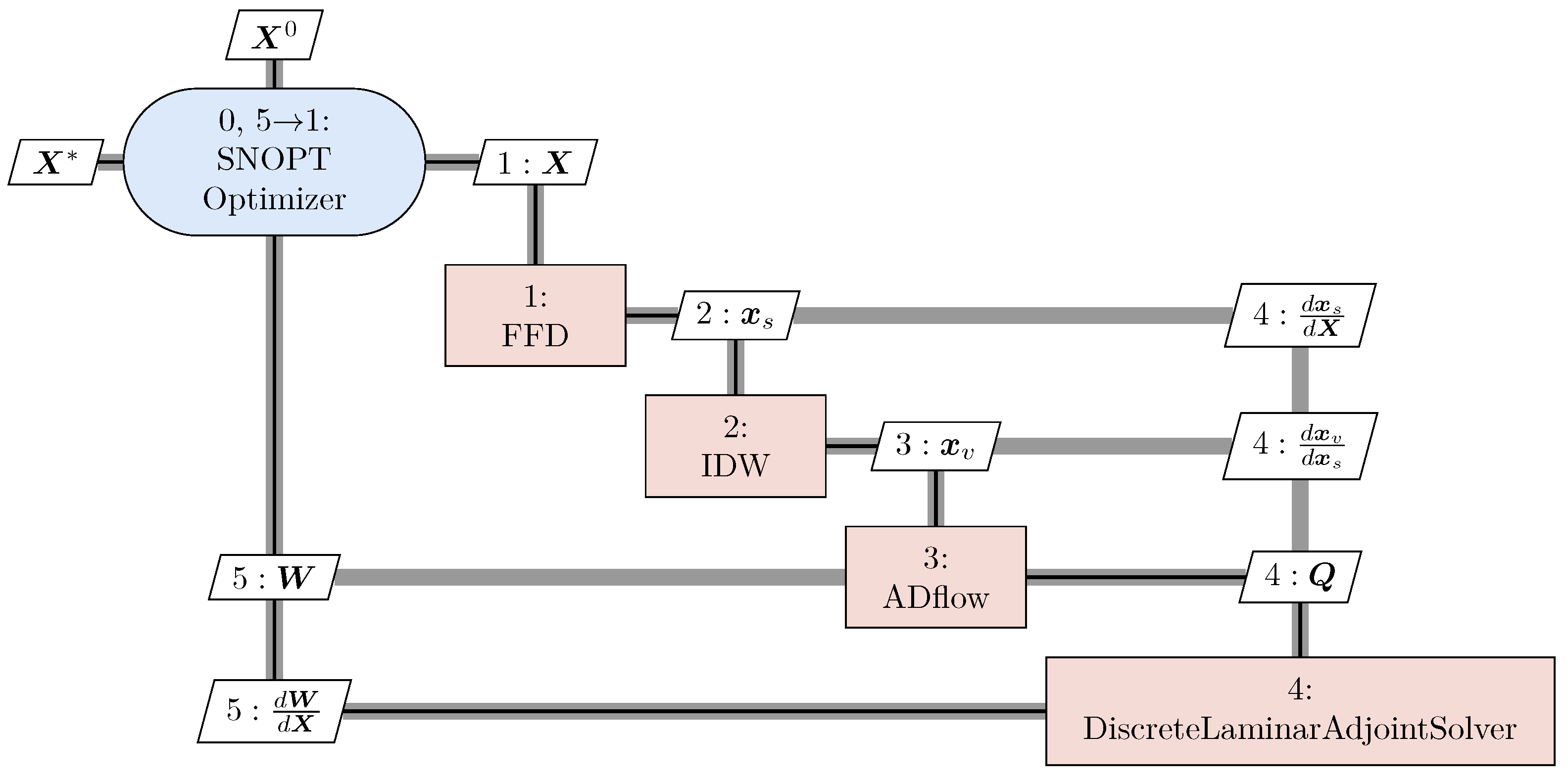
Combined with the auxiliary technology of optimization design, a supersonic wing optimization design system based on discrete adjoint is built, as shown in Figure 5. The optimization process is:
- 1
- Constructing the initial model and the corresponding mesh, and giving the initial design variable ;
- 2
- The surface mesh is parameterized using the FFD method;
- 3
- Based on the deformed surface mesh, the deformed volume mesh is obtained through IDW mesh warping technology;
- 4
- Using ADflow solver to solve the RANS equation to obtain the convergent flow solution vector and the aerodynamic objective function value ;
- 5
- Based on the flow field results, ADflow constructs the adjoint equation and solves it through the GMRES algorithm. Finally, the gradient of the aerodynamic objective function with respect to the design variables is obtained;
- 6
- Combining the calculation results of the flow field in step 4 and the gradient information in step 5, the SNOPT optimization algorithm is used to update the design variables;
- 7
- Repeating steps 2 to 6 until the optimization design converges.
4. Aerodynamic Optimization Design of Subsonic Leading Edge Configuration
4.1. Optimization Problem
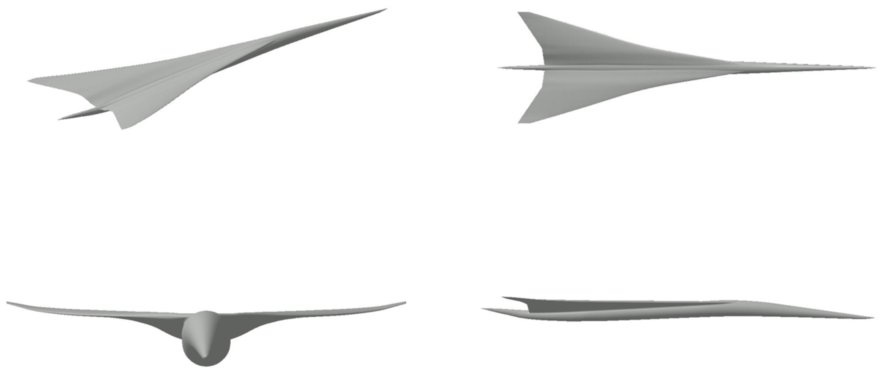
Lockheed Martin (LM) 1021 developed by NASA N + 2 supersonic verification program [24] is selected as the initial configuration, as shown in Figure 6, and the geometric parameters are shown in Table 3 (https://lbpw-ftp.larc.nasa.gov/lbpw1/lm-1021/geometry/ accessed on 3 June 2020).
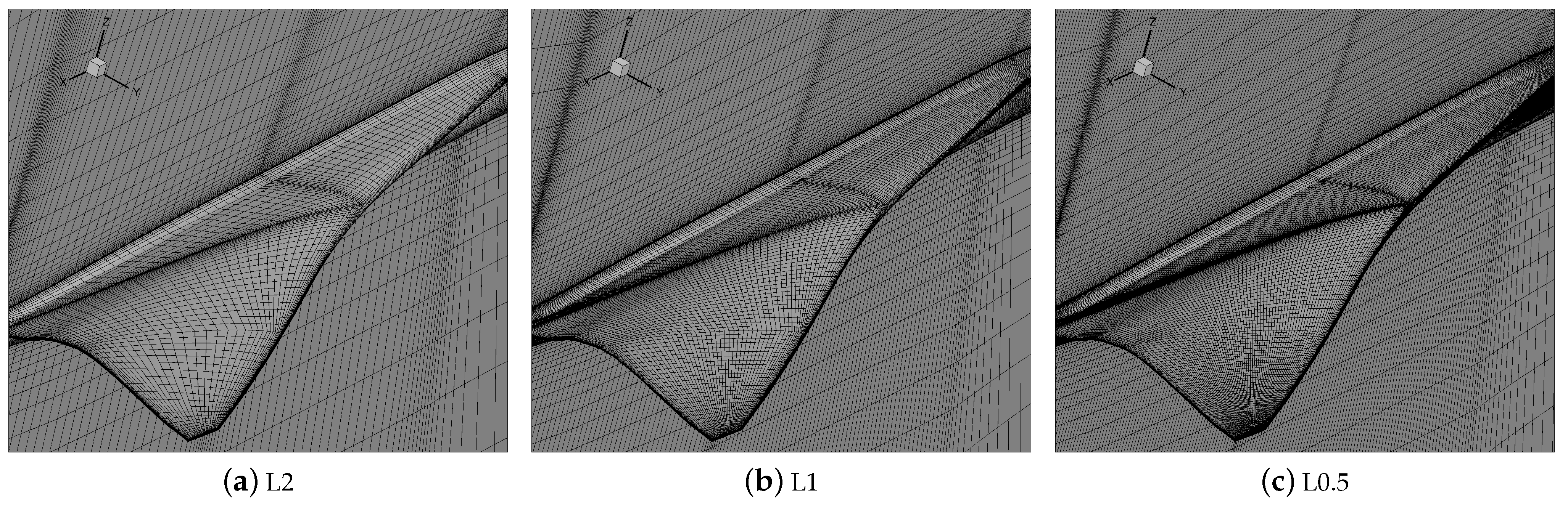
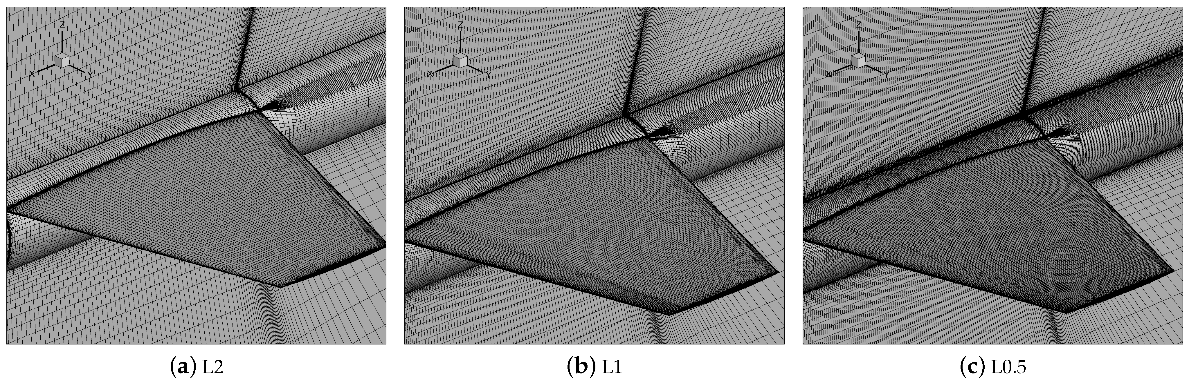
We use commercial software ANSYS-ICEM to generate the structural grid of the initial configuration. A grid convergence study was carried out to determine the resolution accuracy of the grid. To accurately depict the outcomes of grid convergence studies, Roache introduced the Grid Convergence Index (GCI) [45,46]. While it is possible to compute the GCI using two grid levels, it is recommended to use three levels to more accurately determine the order of convergence and ensure that the solutions fall within the asymptotic convergence range. In this research, three grid levels are used, named L2, L1, and L0.5, in which L2 is the most coarse grid, as shown in Figure 7. The GCI between L1 and L0.5 can be defined as follows:
The relative error between the two grids is represented by . In this case, the refinement ratio r is approximately 1.62, and p denotes the order of convergence. The safety factor is given by . Furthermore, the GCI between L2 and L1 can be described as follows.
Table 4 displays the various mesh amount, corresponding drag coefficients, and GCIs, illustrating a converging trend. For each grid level, the solutions should be within the asymptotic range of convergence for the calculated solution. By employing two GCI values computed across three grid levels, this can be verified, as demonstrated in Equation (18).
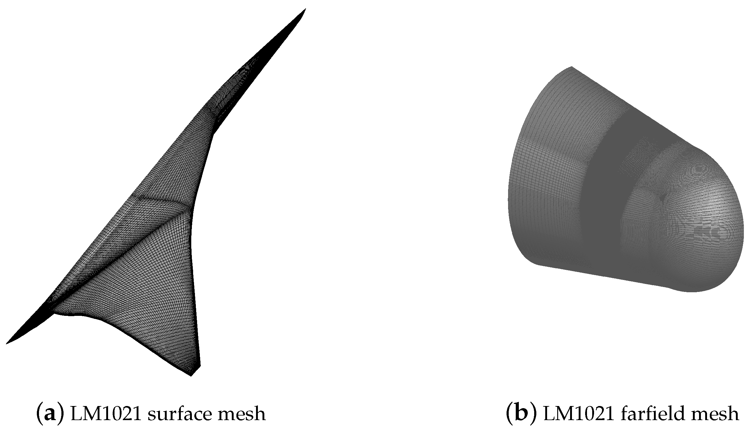
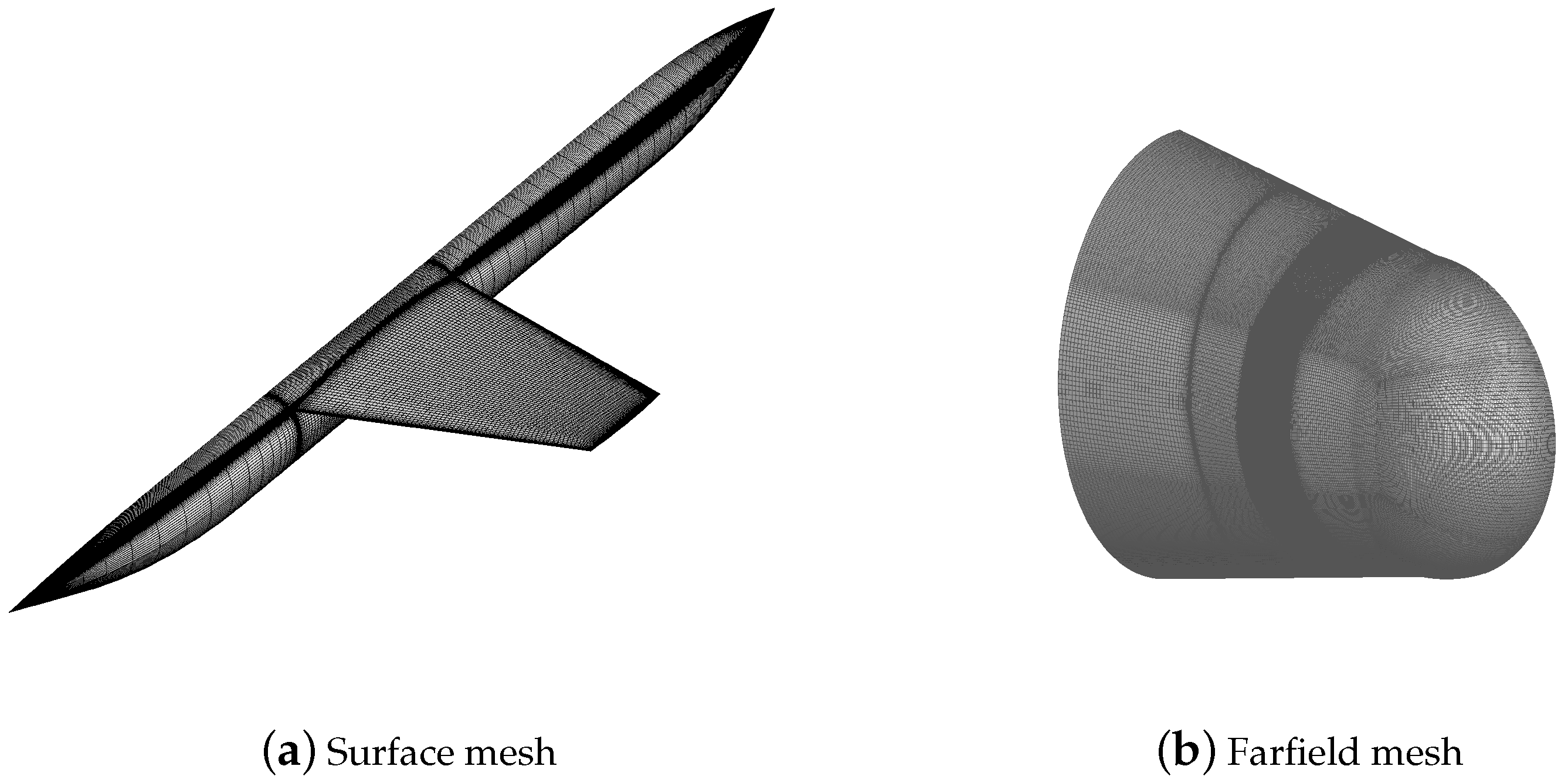
It can be observed that the L1 mesh offers adequate accuracy. Therefore, we use the L1 level in the optimization design. The surface of L1 mesh is shown in Figure 8, the total amount of mesh is 5.3 million, and the height of the first layer of the boundary layer is .
A conical far field whose size is twice the length of the fuselage is used.
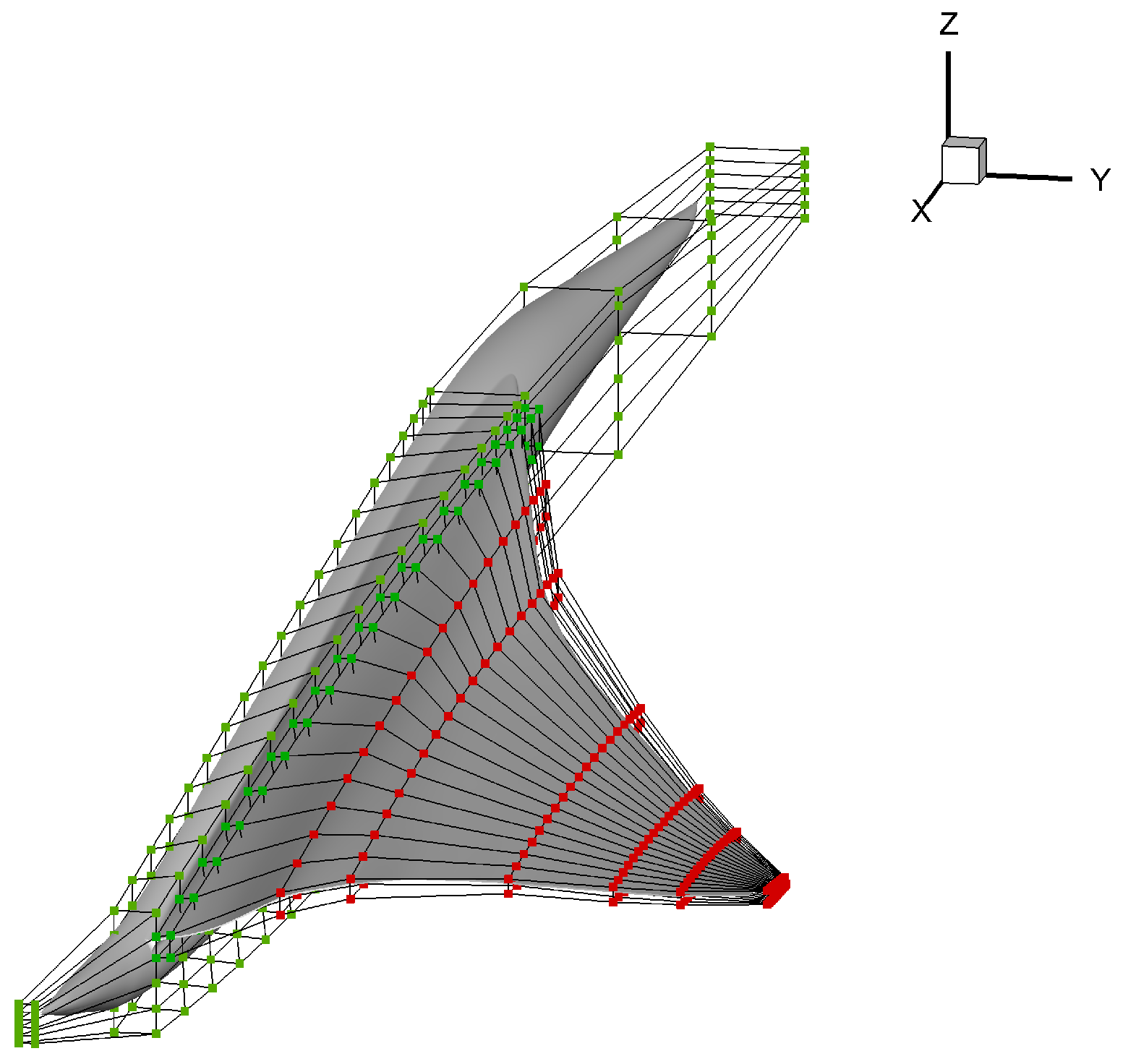
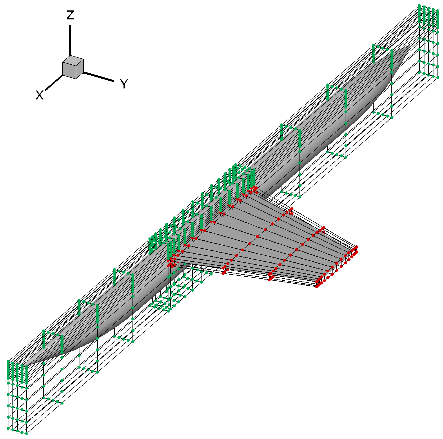
The FFD control frame is shown in Figure 9, where the frame composed of red points is the design variable, and the fuselage and wing root remain unchanged (green points). Meanwhile, the leading and trailing edges of the wing are restricted to remain unchanged too. The parameterization is mainly conducted for the shape deformation of the wing. There are a total of 240 FFD control points on the wing, of which 6 sections are distributed along the span direction, 20 positions are distributed along the chord direction, and 2 layers are in the normal direction. Five sections are selected to twist in the span direction except for the wing root. The deflection of each section is operated by rotating 40 FFD control points at the same span section around a given rotation axis which is always the leading edge.
The design condition is , , . The optimization objective is to minimize the total drag coefficient, and the design variables are the angle of attack, the displacement of FFD control points (a total of 240 design variables) on the wing and five deflection angles of FFD control profile.
Considering engineering application, the wing needs to meet certain structural and volume requirements, so the thickness and volume of the wing must be constrained. Thickness constraints are shown in Figure 10, distributed in seven spanwise positions of the semi-span, and each section is evenly distributed 25 within the range of 5–90% of the chord length. The thickness of each constrained position is not less than 97% of the initial configuration thickness. The volume constraints are defined between 50 cross-sectional positions in the semi-span. There are 25 parts in each cross-section within the range of 20–70% of the chord length so as to ensure that the volume of the optimized wing is not smaller than that of the initial configuration.
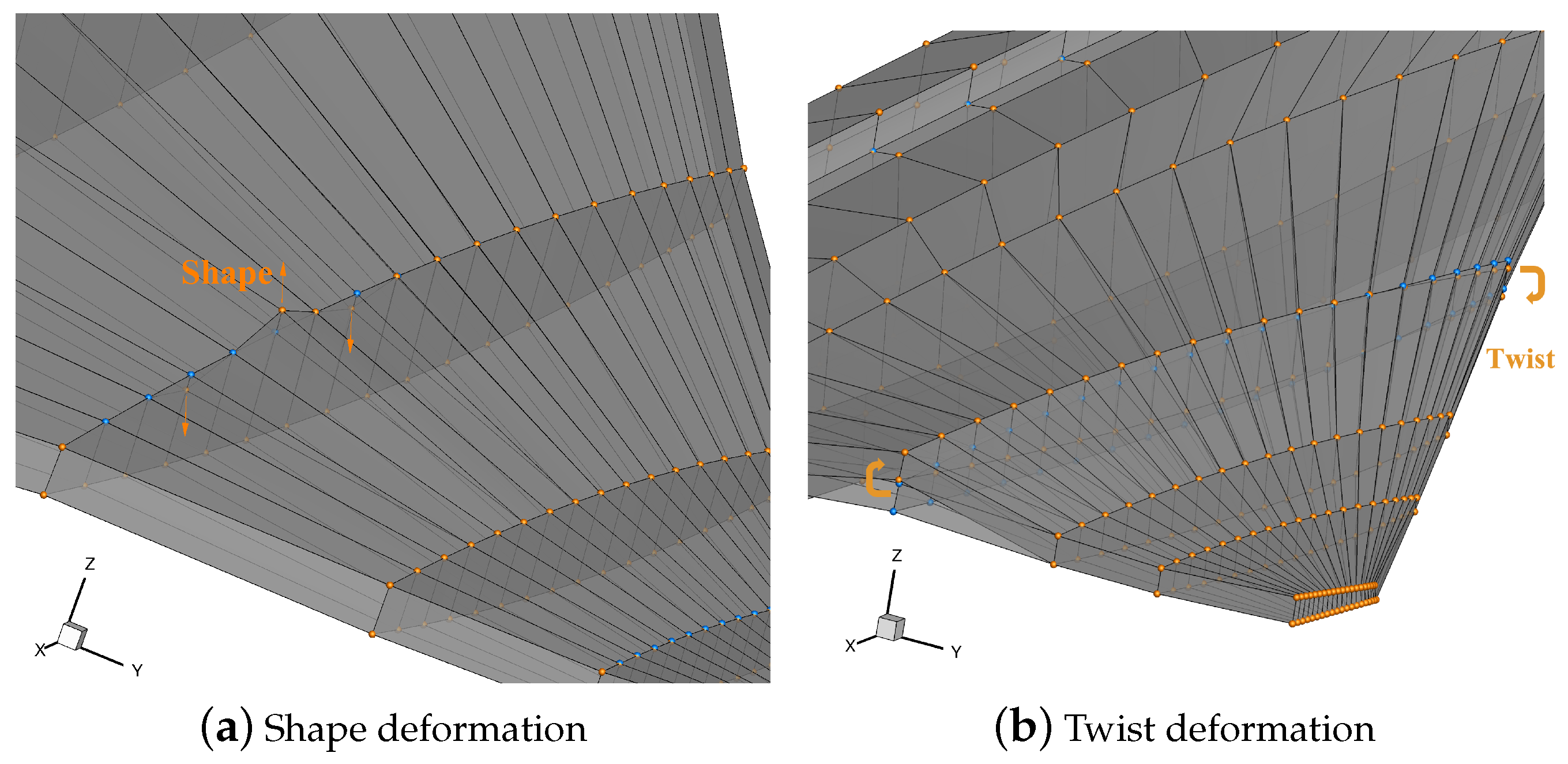
Without the pitch moment constraint, the optimizer would add a pitch moment that is unfavorable to the trim drag, thereby affecting the overall design of the aircraft. Therefore, the pitch moment constraint is crucial for a feasible result. We restrict the pitching moment coefficient to a range not less than 0. Overall, the optimization problem settings are shown in Table 5. To clarify, the specific moving characteristics of the FFD frame of the shape deformation and the twist deformation are shown in Figure 11. The shape deformation is that the FFD control points move in the z-direction to change the geometry. For twist deformation, each FFD control profile along the y direction can be twisted around a fixed axis so that the airfoil profiles can be geometrically twisted to change the local angle of attack. We totally conducted two kinds of optimization for the subsonic leading edge configuration. The first one is the optimization with only shape variables. The second one is the optimization with both shape variables and twist variables. When performing shape+twist optimization, the deformation of the FFD frame is also the coupling of the two deformation forms.
4.2. Optimization Results
The optimized design is, respectively, carried out under the condition of whether there are twist variables. The comparison of aerodynamic force coefficients before and after optimization is shown in Table 6. The optimization results show that the optimized configuration with twist variables (Twist + Shape) can obtain greater drag reduction, and the total drag coefficient is reduced by 5.78 counts compared with the initial configuration, a reduction of 3.78%. Compared with the initial configuration, the total drag coefficient of the optimized configuration without twist variables (Shape) is reduced by 3.87 counts, a decrease of 2.53%. The change in the angle of attack, which is also used as a design variable, is small in the optimization process. Meanwhile, the pitching moment coefficient remains basically unchanged, which satisfies the constraints.
The distribution of spanwise lift load and twist angle between the optimized configuration and the initial configuration is shown in Figure 12. Compared with the initial configuration, the two optimal configurations both show an increasing lift load in the inner wing and a decreasing lift load in the outer wing so that the distribution of lift load is closer to the elliptical distribution, which can effectively reduce the induced drag. The geometric twist has a more significant effect on adjusting the spanwise lift load distribution and reducing the induced drag.
The comparison of spanwise drag distribution before and after optimization is shown in Figure 13. Compared with the initial configuration, the optimized configuration adding twist variables has obvious changes, corresponding to the change trend of spanwise lift load and twist angle. Correspondingly, the large positive twist angle of the outer wing leads to a local drag penalty, but the tendency of the load to move outward is conducive to the effective improvement of the overall performance.
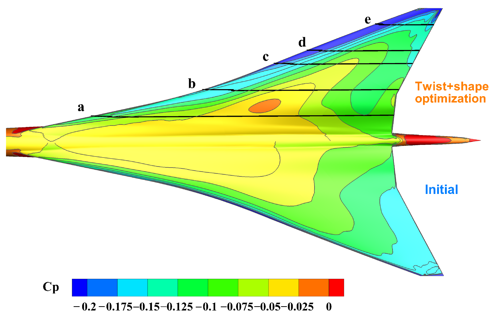
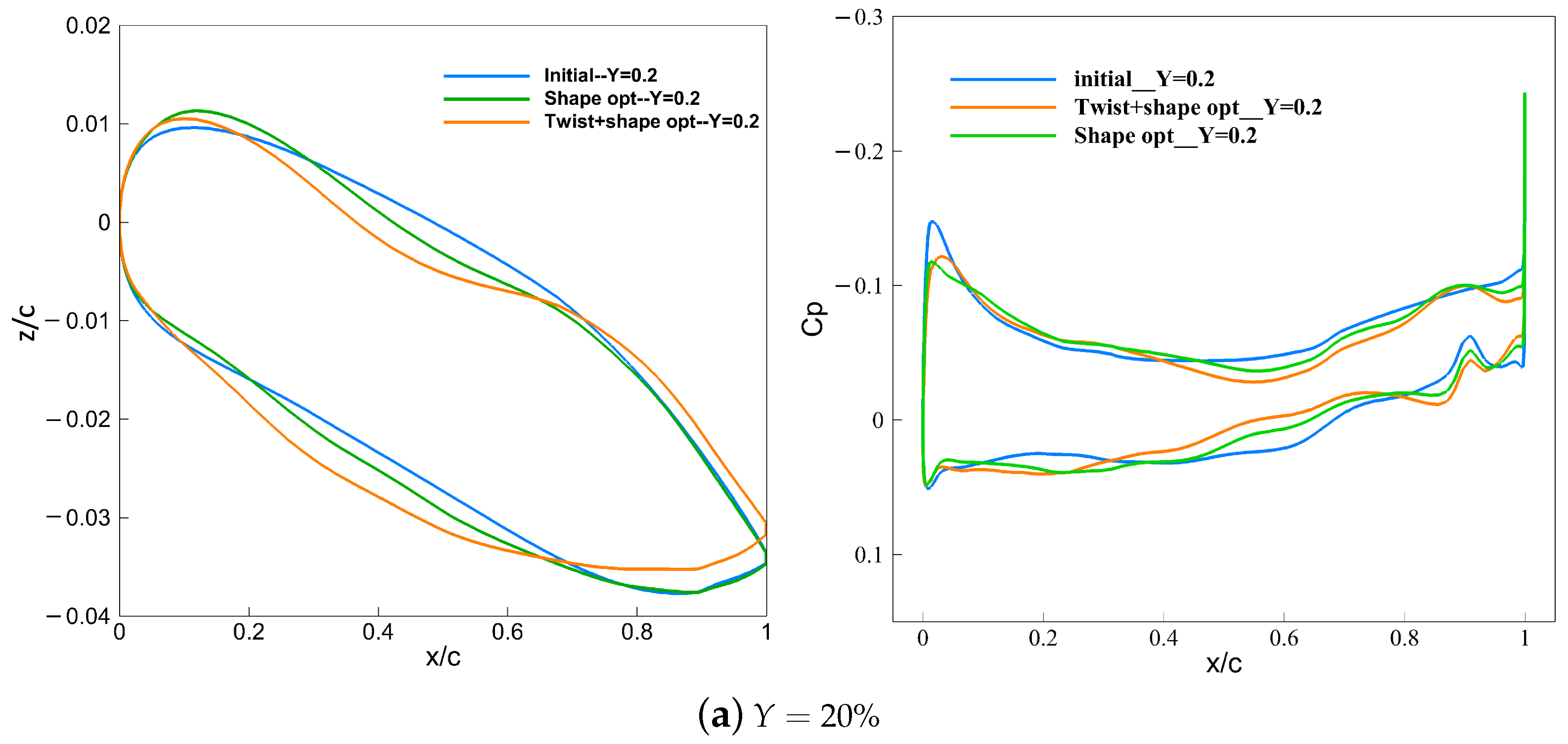
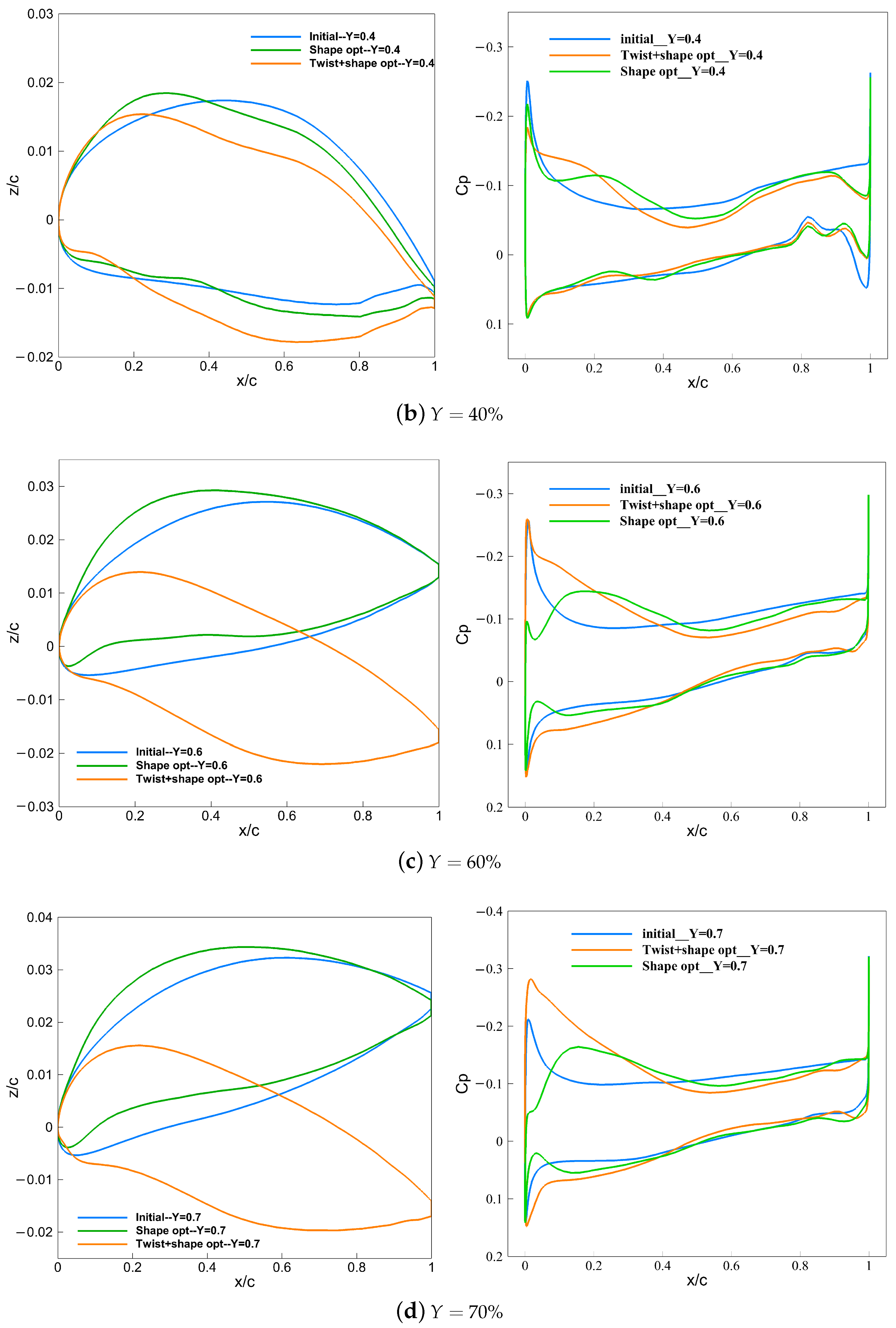
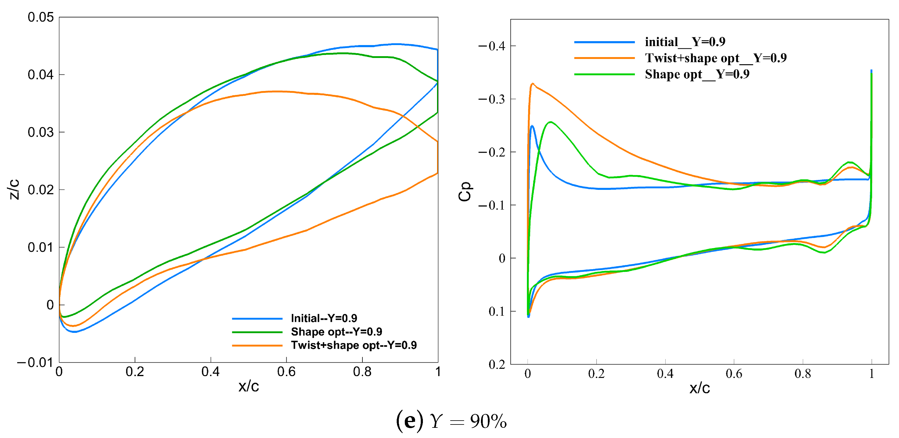
Figure 14 shows the contour of the pressure coefficient on the upper surface of the wing with the optimized configuration and the initial configuration. Corresponding to Figure 15, a-e represents the slices in the spanwise direction, respectively .
The comparison of the surface pressure distribution and the airfoil in a typical section before and after optimization is shown in Figure 15. In the inner wing, unloading is mainly achieved in two ways. On the one hand, increasing the curvature radius of the leading edge weakens the peak suction force and decreases the adverse pressure gradient, which is beneficial to the reduction in pressure drag. On the other hand, the unloading of the inner wing section is achieved by reducing the camber of the middle and rear sections of the airfoil. In the outer wing section, the optimized configuration with twist variables mainly increases the lift load with a large positive twist angle, while the optimized configuration without twist variables only changes the shape of airfoil; for instance, increasing the camber of the airfoil.
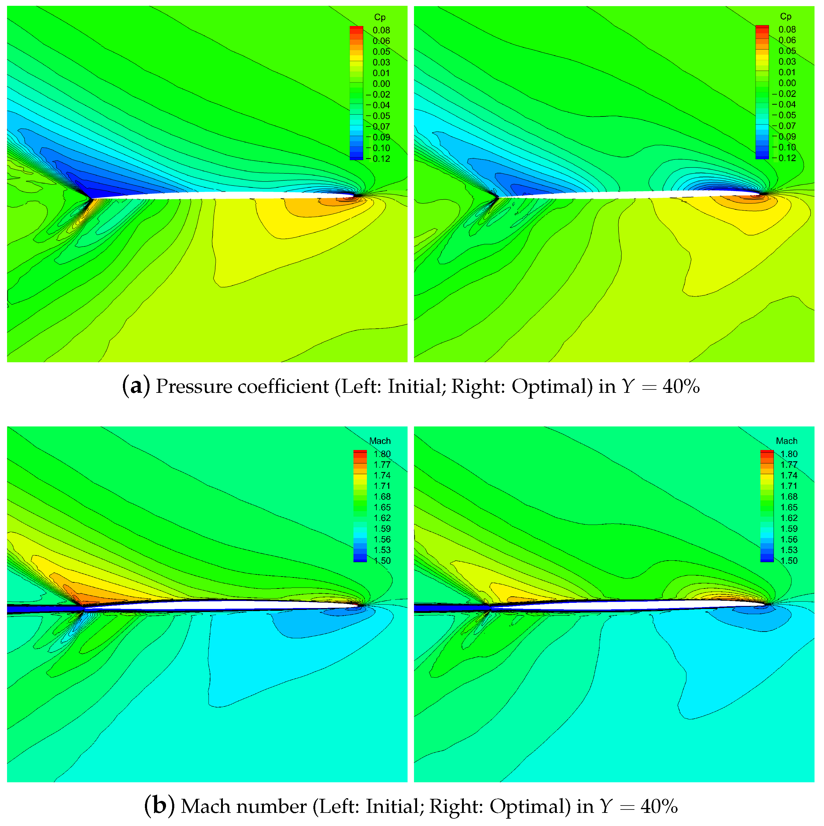
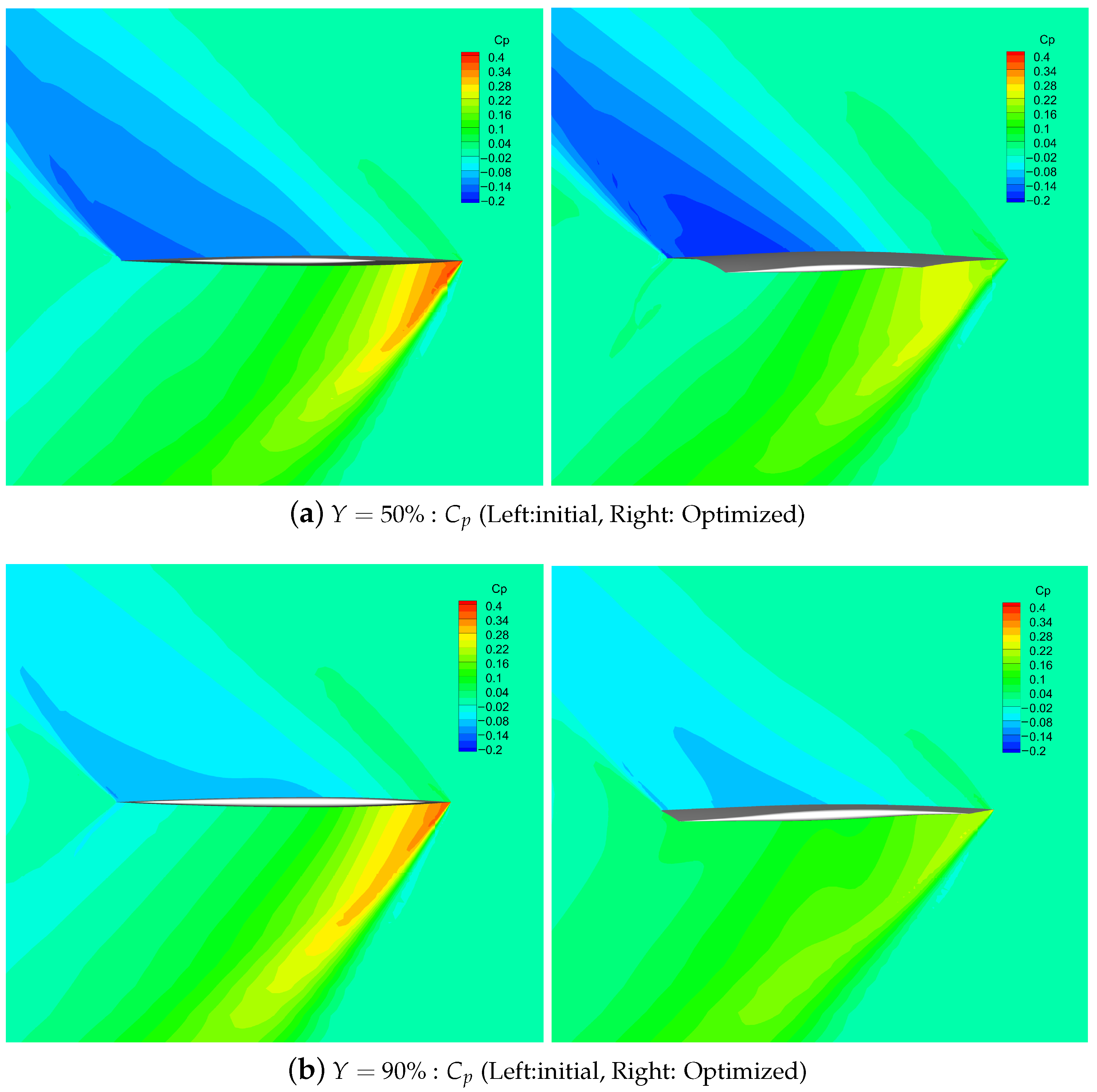
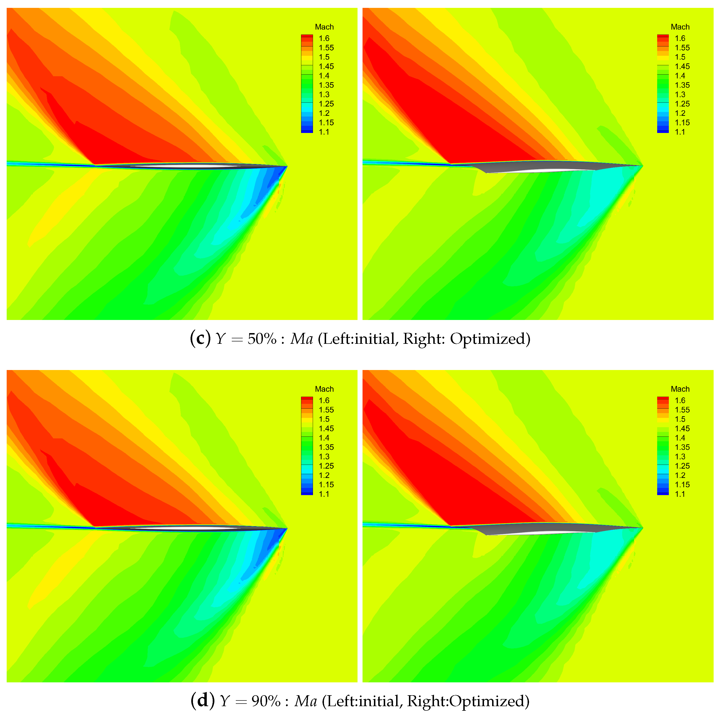
The spatial distribution of the pressure coefficient and Mach number of the typical spanwise section of the initial configuration and the optimized configuration with twist variables are shown in Figure 16. Compared with the initial configuration, the spatial pressure recovery near the upper surface of the trailing edge of the optimized configuration is more gentle, which can effectively reduce the wave drag. Meanwhile, the spatial areas with extreme negative pressure (dark blue part in Figure 16) on the upper surface of the optimized configuration are reduced at the tailing edge of the wing, and they all move forward along the chord direction. Corresponding to the trend of the wing lift load moving towards the leading edge and the outer wing section, the spatial areas with extreme negative pressure near the upper surface of the leading edge gradually increase from the inner wing section along the span direction.
The spatial distribution of the Mach number before and after optimization has the same change pattern. Compared with the initial configuration, the spatial areas with a high Mach number (dark red part in Figure 16) of the optimized configuration are reduced at the tail of the wing and move forward along the chord direction. Meanwhile, the high Mach number region near the upper surface of the leading edge gradually increases from the inner wing section along the spanwise direction.
For a supersonic wing with a subsonic leading edge, the airflow velocity increases continuously from the leading edge to the trailing edge, so there are obvious compression waves in the space near the trailing edge. At the trailing edge of the inner wing section, the spatial pressure coefficient changes significantly before and after optimization, so we slice the pressure coefficient distribution and mach distribution at the 40% position. As shown in Figure 17, the contour lines of pressure coefficient and Mach number at the tail of the upper surface of the optimized configuration are both sparser than those of the initial configuration, indicating that the compression wave intensity is reduced after optimization, thereby reducing the wave drag.
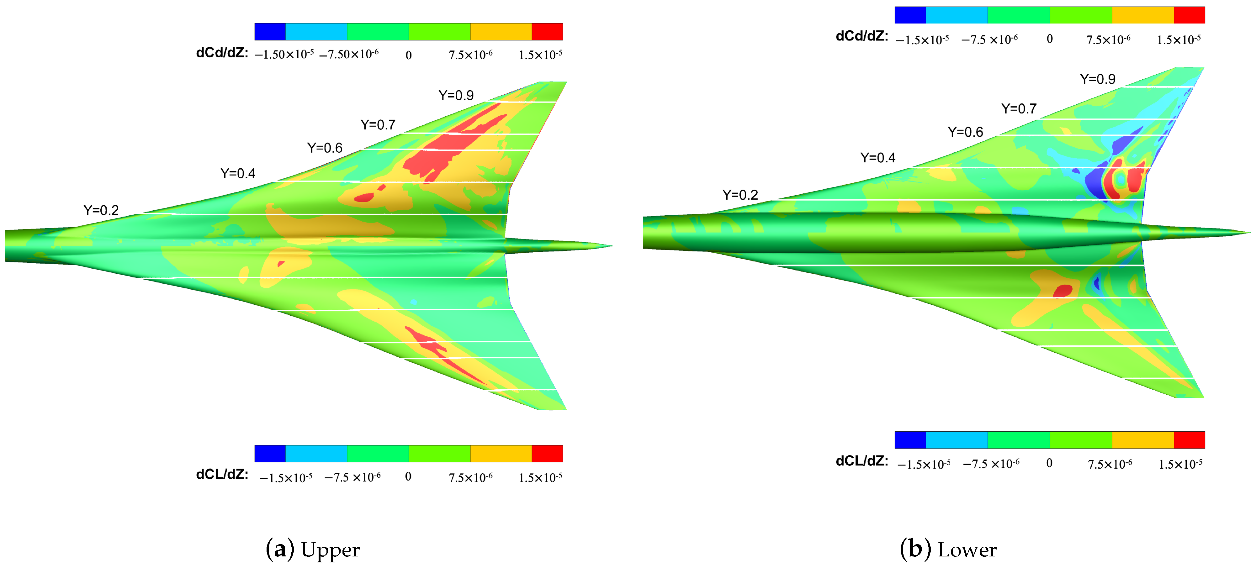
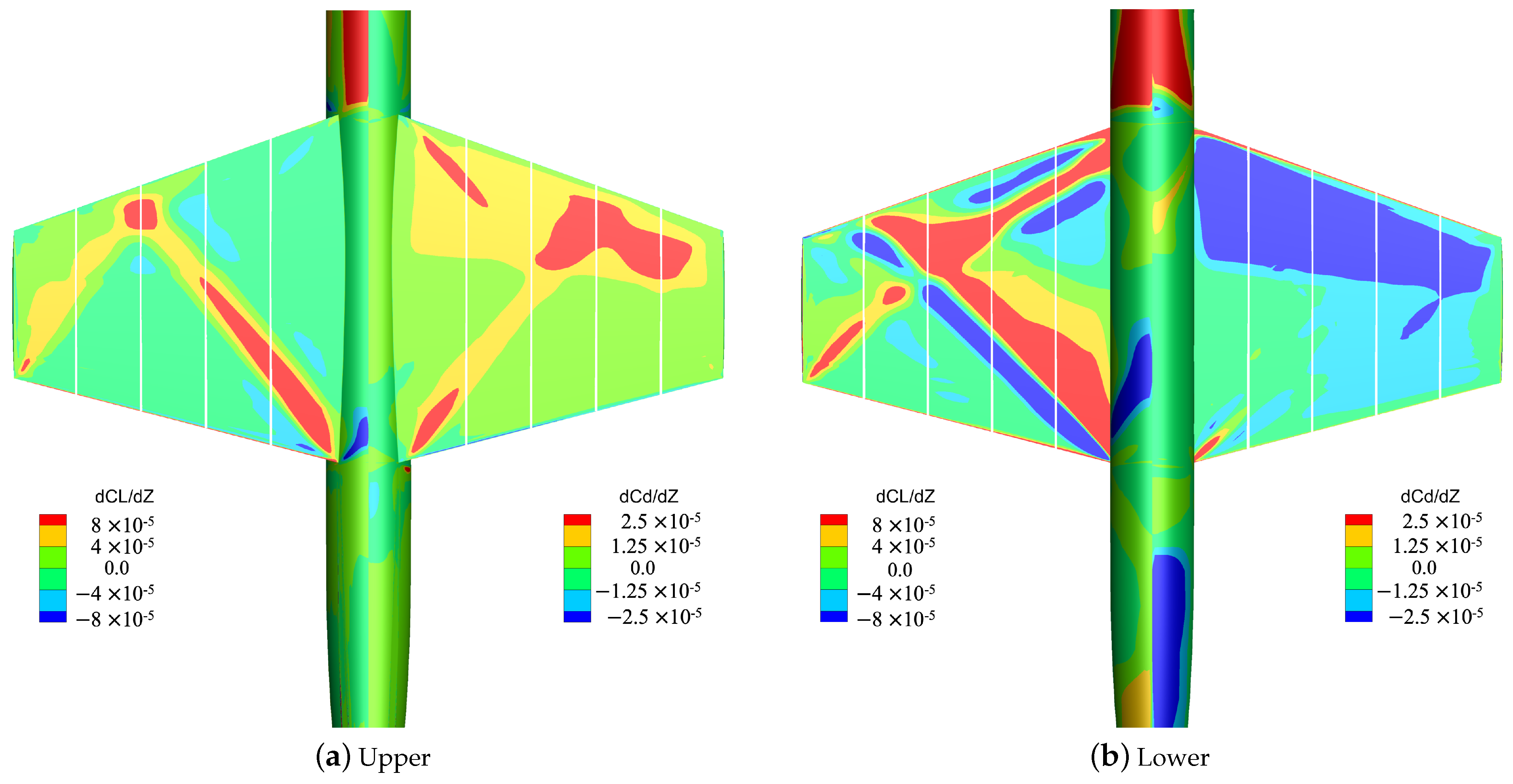
In order to qualitatively analyze the trade-off between lift and drag, as well as airfoil deformation and constraints in the aerodynamic optimization design, sensitivity analysis is performed using the gradient information obtained from the discrete adjoint equation for the initial configuration. The derivative distribution of the lift/drag coefficients of the upper and lower surfaces with respect to the displacement of the surface grid cells is shown in Figure 18, where the displacement direction is positive along the positive direction of the coordinate axis.
Comparing the most sensitive area of the lift and drag coefficients to the deformation of the airfoil, it can be found that the dark red and dark blue areas of the drag coefficient are larger than those of the lift coefficient in both the upper and lower surface, indicating that when the upper and lower surface deforms along the z axis, it will have a greater impact on the drag coefficient. On the other hand, the dark red and dark blue areas of the upper surface are more than those of the lower surface, indicating that as the airfoil surface deforms along the axis, it has a greater effect on the upper surface than the lower surface. Figure 18 only shows the sensitivity of the aerodynamic function with respect to the change of the surface grid, and the aerodynamic constraints and geometric constraints must be considered in the actual engineering design. Therefore, the optimization algorithm will combine the sensitivity information with the constraints to obtain the most feasible direction of optimization.
According to the comparison of section airfoils before and after optimization (Figure 15), it can be observed that in the optimized configuration, the upper and lower surfaces of each section airfoil deforms along the negative direction of the z axis compared with the initial configuration. Combined with the analysis results of sensitivity, when the upper surface deforms along the negative direction of the z axis, the drag coefficient decreases accordingly, and the drag reduction effect is more significant. Although this deformation trend may lead to a decrease in the lift, large-scale changes in the surface profile can only cause small-scale fluctuations in the lift. Therefore, the optimizer prefers to reduce the drag, which is the dominant direction of optimization, and through the deformation of the local profile ensure that the lift constraint is satisfied.
On the other hand, according to the sensitivity analysis results, the movement of the lower surface of the airfoil along the positive direction of the z axis reduces the drag coefficient; but the actual optimization shows adverse results. The reason is that the drag coefficient is more sensitive to the deformation of the upper surface than to the deformation of the lower surface. On the balance, the optimizer mainly focuses on the upper surface deformation. At the same time, the lower surface is followed to deform according to the deformation of the upper surface so that the final design results satisfy the thickness and volume constraints.
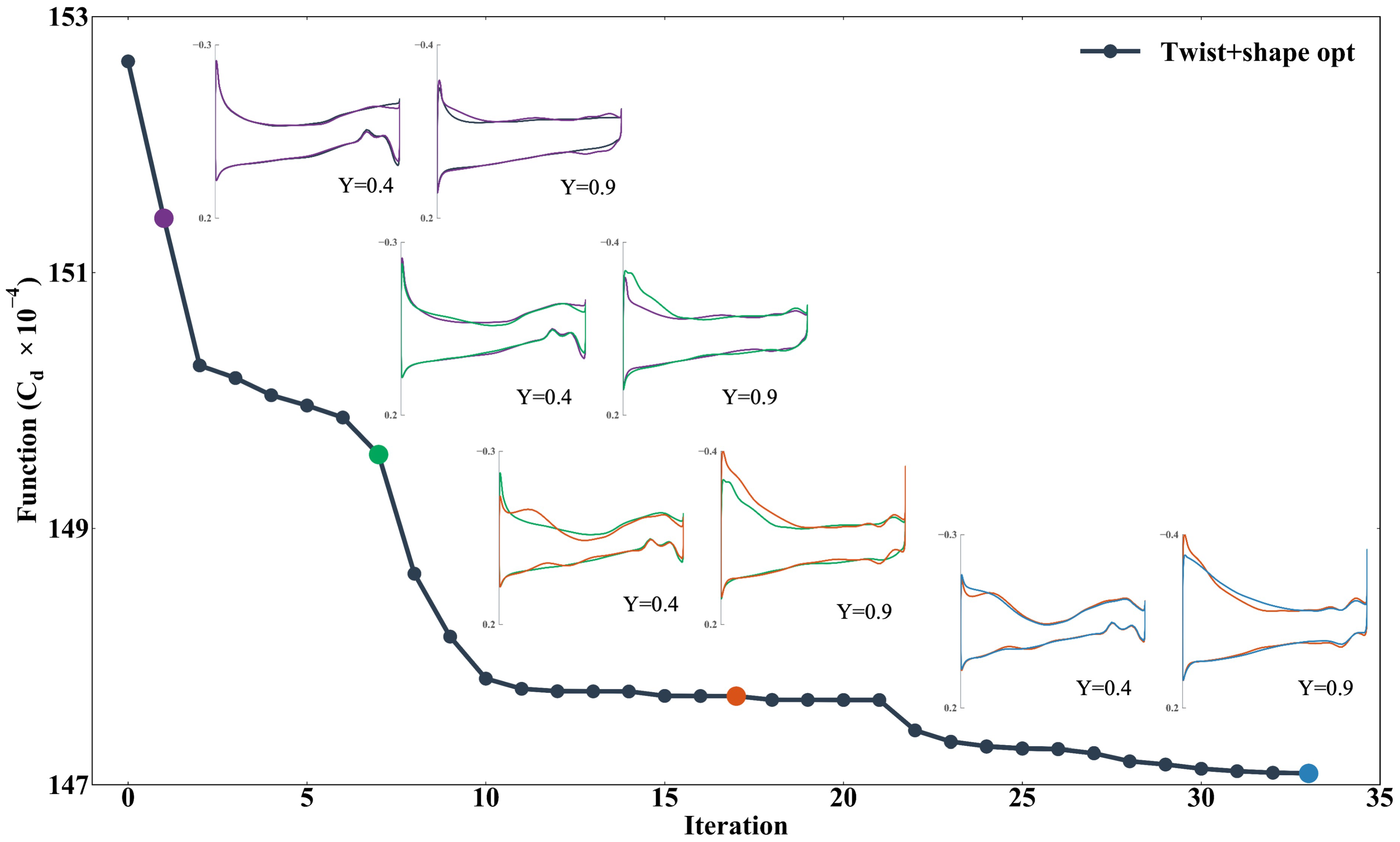
The convergence history of the optimization is shown in Figure 19. The intermediate process of the pressure distribution at the typical sections of the inner wing section and the outer wing section from the initial configuration to the final optimized configuration is given, respectively. After 33 main iterations, the constraints and the convergence conditions of the objective function are met. From the convergence process of the main iteration, the drag coefficient is reduced quickly in the first 10 main iterations of the gradient-based optimization. In the final stage, the drag reduction is small and the optimizer mainly focuses on smoothing the pressure distribution. The optimization process gradually achieves the lift load moves from the inner wing section to the outer wing section.
5. Aerodynamic Optimization Design of Supersonic Leading Edge Configuration
5.1. Optimization Problem
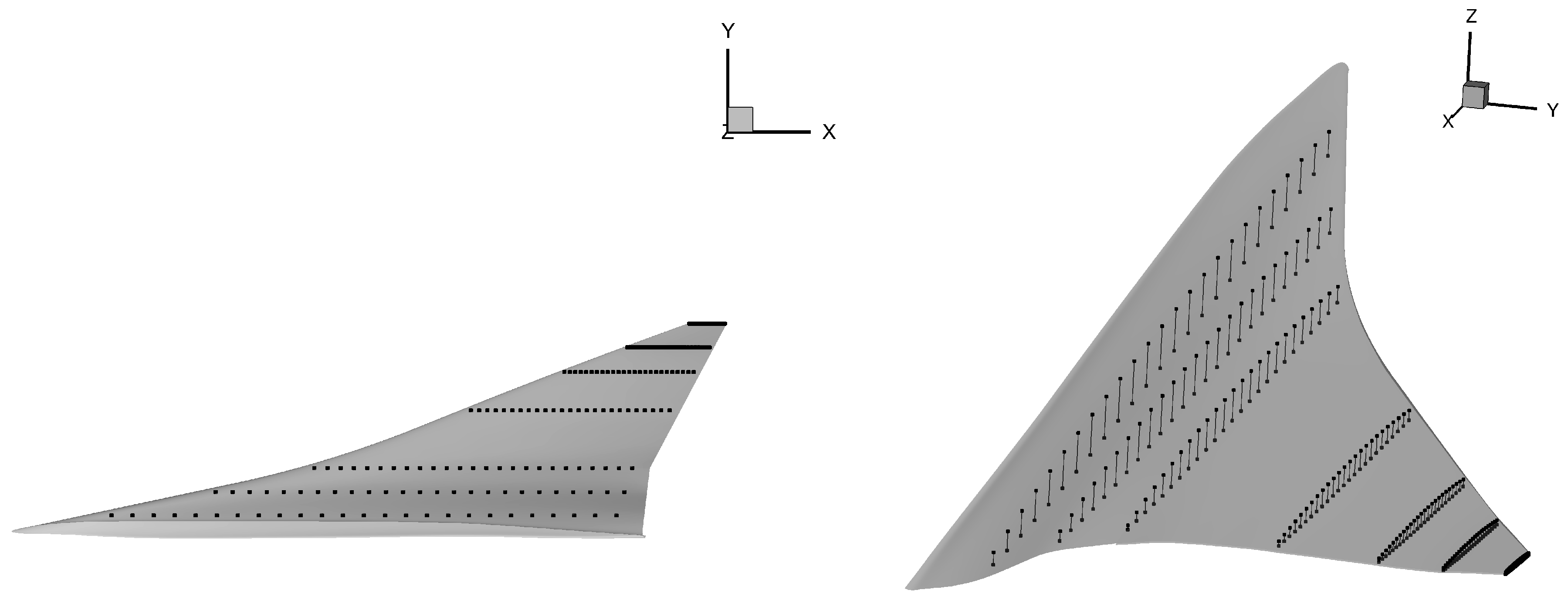
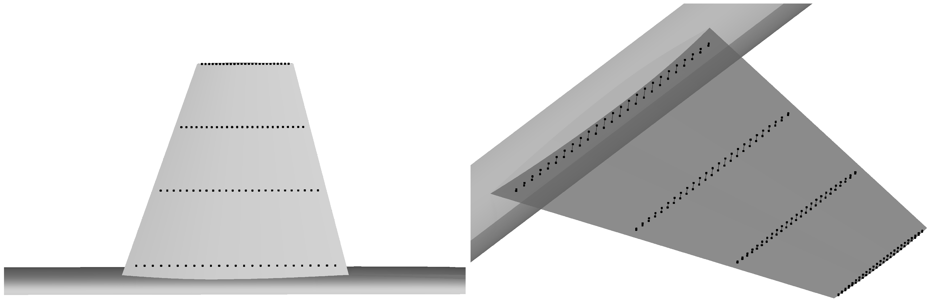
We define a simple trapezoidal wing, as shown in Figure 20, as the initial configuration referring to the design scheme of Aerion AS2, and the geometric parameters are shown in Table 7.
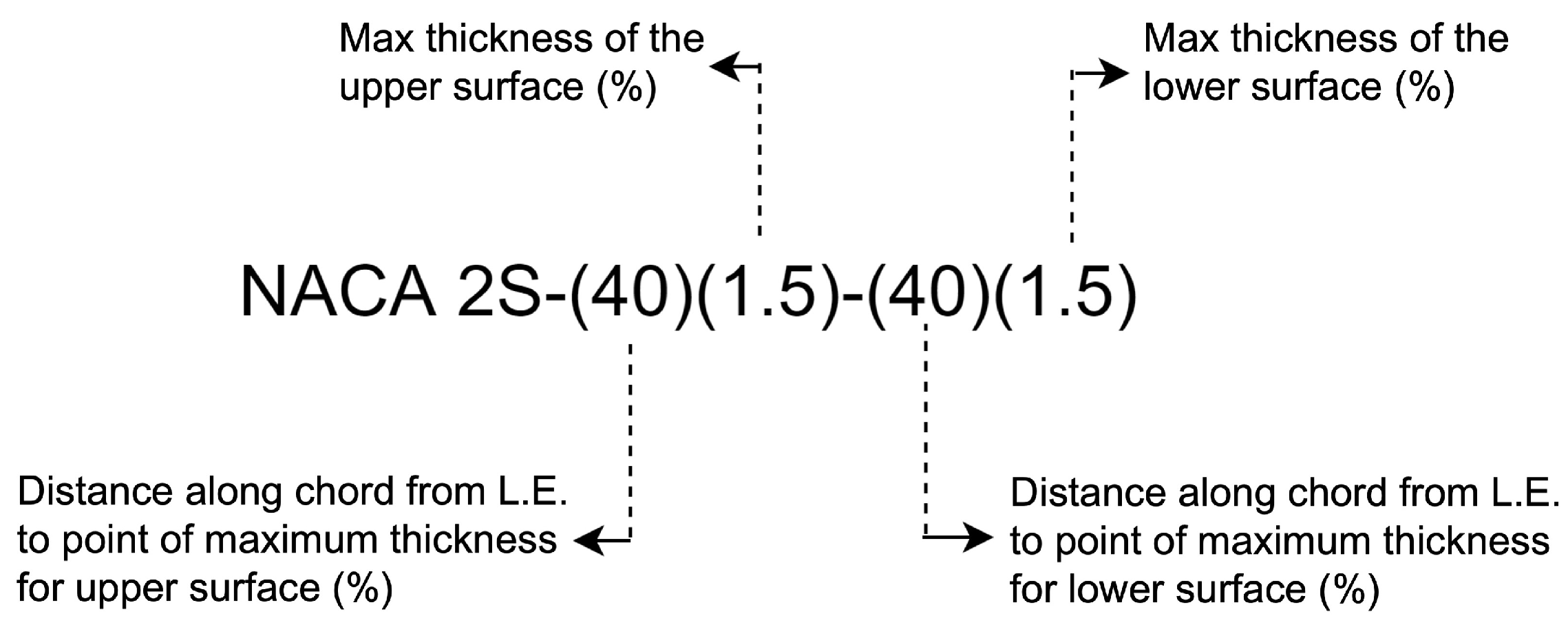
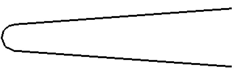
The double-circular-arc supersonic airfoil NACA 2S-(40)(1.5)-(40)(1.5) is used, and its parameters are defined as shown in Figure 21. The existence of a sharp leading edge of a typical supersonic airfoil has an adverse effect on the geometric deformation. The displacement of the FFD control point can make the smooth arc sharp, but because the initial surface is not continuous by order, the reverse process cannot be accomplished. Therefore, we use a small arc instead of the ideal sharp leading edge. The diameter of the small arc is 0.4 mm. The blunted leading edge of the airfoil is shown in Figure 22.
ANSYS-ICEM is used to generate the structural grid of the initial configuration, as shown in Figure 23. Likewise, a grid convergence study is performed on the supersonic leading edge configuration. Figure 24 shows three levels of grids, where the grid is refined from L2 to L0.5. The different mesh amounts, related drag coefficients, and GCIs based on Equations (17) and (19) are shown in Table 8 to show a converging tendency, where the refinement ratio r is 1.29. The solutions should fall within the estimated solution’s asymptotic range of convergence for each grid level. This can be confirmed by using two GCI values calculated over three grid levels, as shown in Equation (20).
Considering the solving efficiency, L1 mesh is utilized in our optimization design, which can provide the solution with sufficient accuracy. The amount of L1 mesh is 6.3 million, and the height of the first layer of the boundary layer is . A conical far field whose size is twice the length of the fuselage is used, as shown in Figure 23.
The FFD control frame is shown in Figure 25, where the red control points are chosen as design variables. The fuselage and wing root remain unchanged, and the leading and trailing edges of the wing are also restricted to remain unchanged (green points). The parameterization is mainly conducted for the shape deformation of the wing. For the wing profile deformation, there are a total of 120 FFD control points, of which four sections are distributed along the span direction, 15 positions are distributed along the chord direction, and two layers are in the normal direction. We select three stations in the span direction except the wing root to control the twist of the wing section and achieve the deflection of each station by rotating the 30 FFD control points at the same span location around a given rotation axis, which is always the leading edge.
The design condition is , , . The optimization objective is to minimize the total drag coefficient, and the design variables are the angle of attack, the displacement of FFD control points (a total of 120 design variables) on the wing and three deflection angles of FFD control profile.
Considering engineering application, the thickness and volume of the wing are also constrained. Thickness constraints are shown in Figure 26, distributed in four spanwise positions of the semi-span. There are 25 parts uniformly distributed in each section within the range of 5–90% chord length. To compare the optimized configurations under different thickness constraints, the optimal design is carried out under the condition that the thickness constraints are, respectively, and . The volume constraints are distributed in the same way as that of the subsonic leading edge configuration. In order to avoid the adverse affect, the pitching moment coefficient is constrained within a range not less than 0. The optimization problem statement for supersonic leading edge configuration is shown in Table 9.
5.2. Optimization Results
The comparison of aerodynamic force coefficients between the optimized configuration and the initial configuration is shown in Table 10, where Opt_0.7t represents the optimized configuration with a thickness constraint of , and Opt_0.9t represents the optimized configuration with a thickness constraint of .
Compared with the initial configuration, the drag coefficient of the Opt_0.7t optimized configuration is reduced by 13.04 counts, a decrease of 4.53%. The drag coefficient of the Opt_0.9t optimized configuration is reduced by 10.1 counts, a decrease of 3.51%. In the optimization process, the angle of attack is also used as a design variable. Compared with the initial configuration, the angle of attack of the optimized configuration of Opt_0.7t and Opt_0.9t increases by 0.03 and 0.01, respectively, which are small. Meanwhile, the pitching moment coefficient changes slightly before and after optimization, which satisfies the pitching moment constraint.
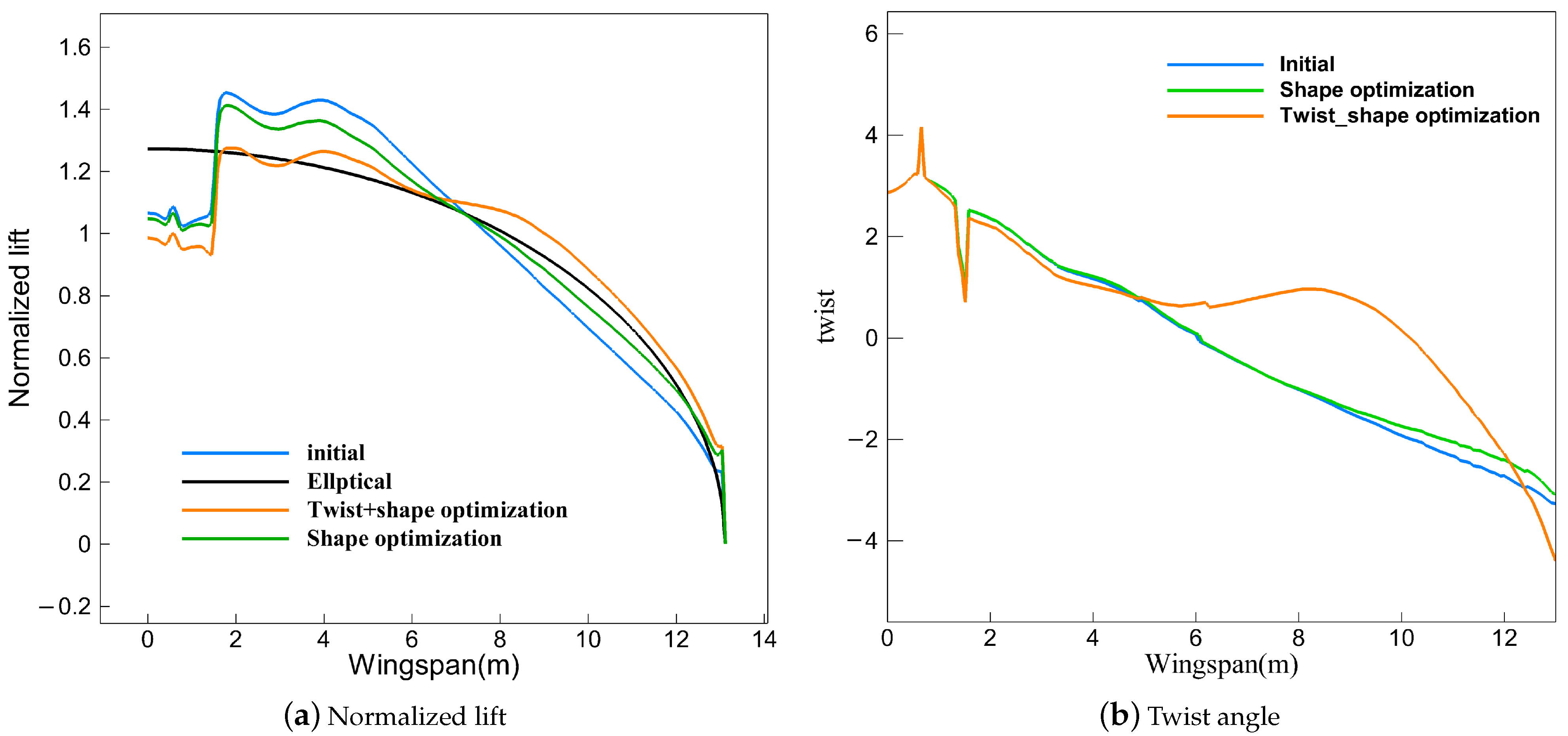
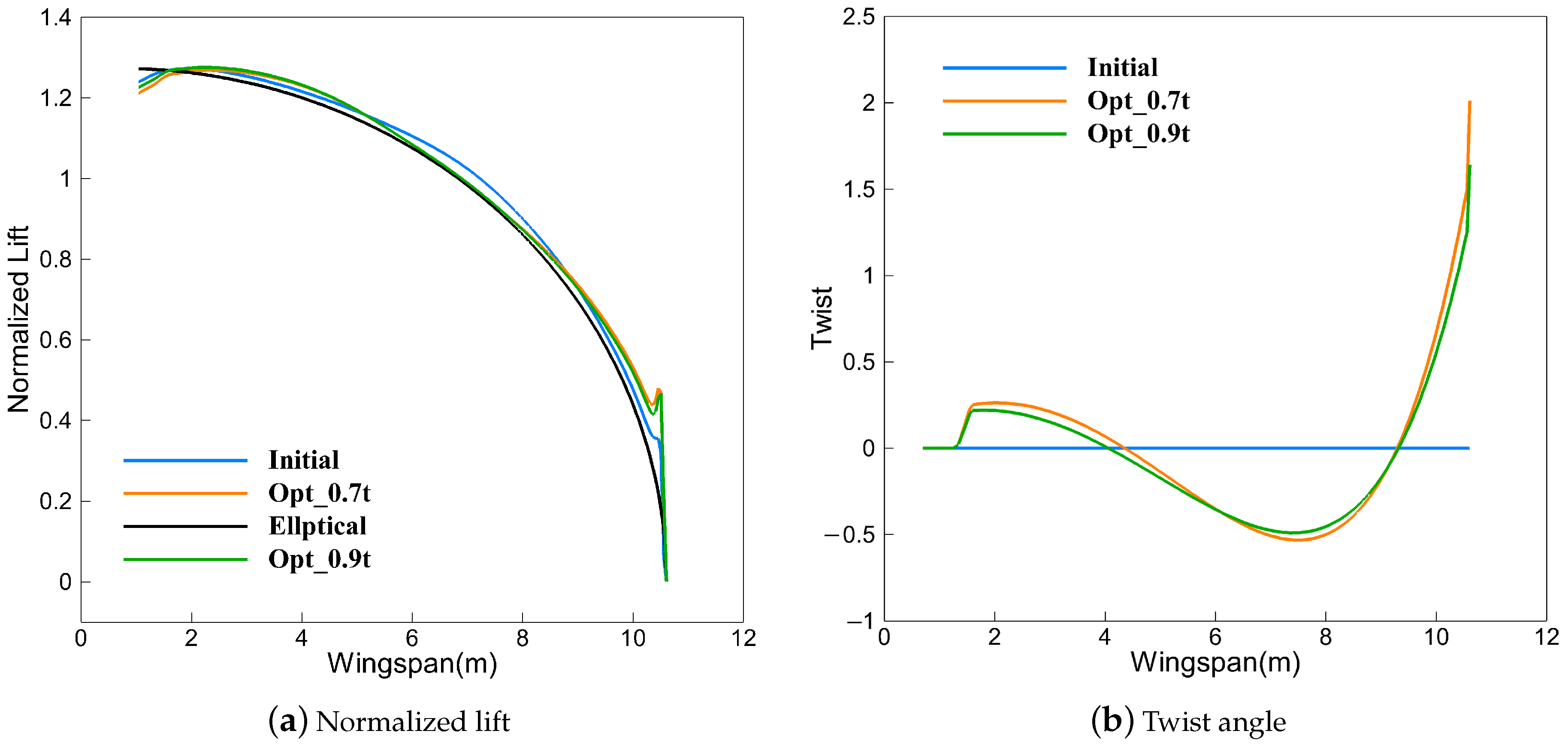
The comparison of normalized lift and twist angle distribution along the span direction before and after optimization is shown in Figure 27. Since the initial configuration is the spanwise chord length distribution of the trapezoidal plane, the initial lift load is close to the elliptical distribution, which is an ideal distribution to reduce the induced drag. However, the lift distribution of the two optimized configurations shows a tendency to deviate from the elliptical lift distribution. Therefore, unlike the subsonic leading edge configuration, the supersonic leading edge configuration takes reducing shock wave drag as the optimization dominant direction. Compared with the initial configuration, the lift in the optimized configuration increases in the inner wing section. It decreases nonlinearly in the middle wing section, which is close to an elliptical lift distribution. In the outer wing section, the lift gradually increases, and the overall lift load is transferred to the wing root and wing tip.
Corresponding to the changing trend of lift, while the middle wing section is negatively twisted, both the inner wing section and the outer wing section have positive twist angles, and the lift is influenced by the local angle of attack. Moreover, the changing trend of the twist angle under the two thickness constraints is the same compared with the initial configuration, and there is only a slight difference in the amount of change.
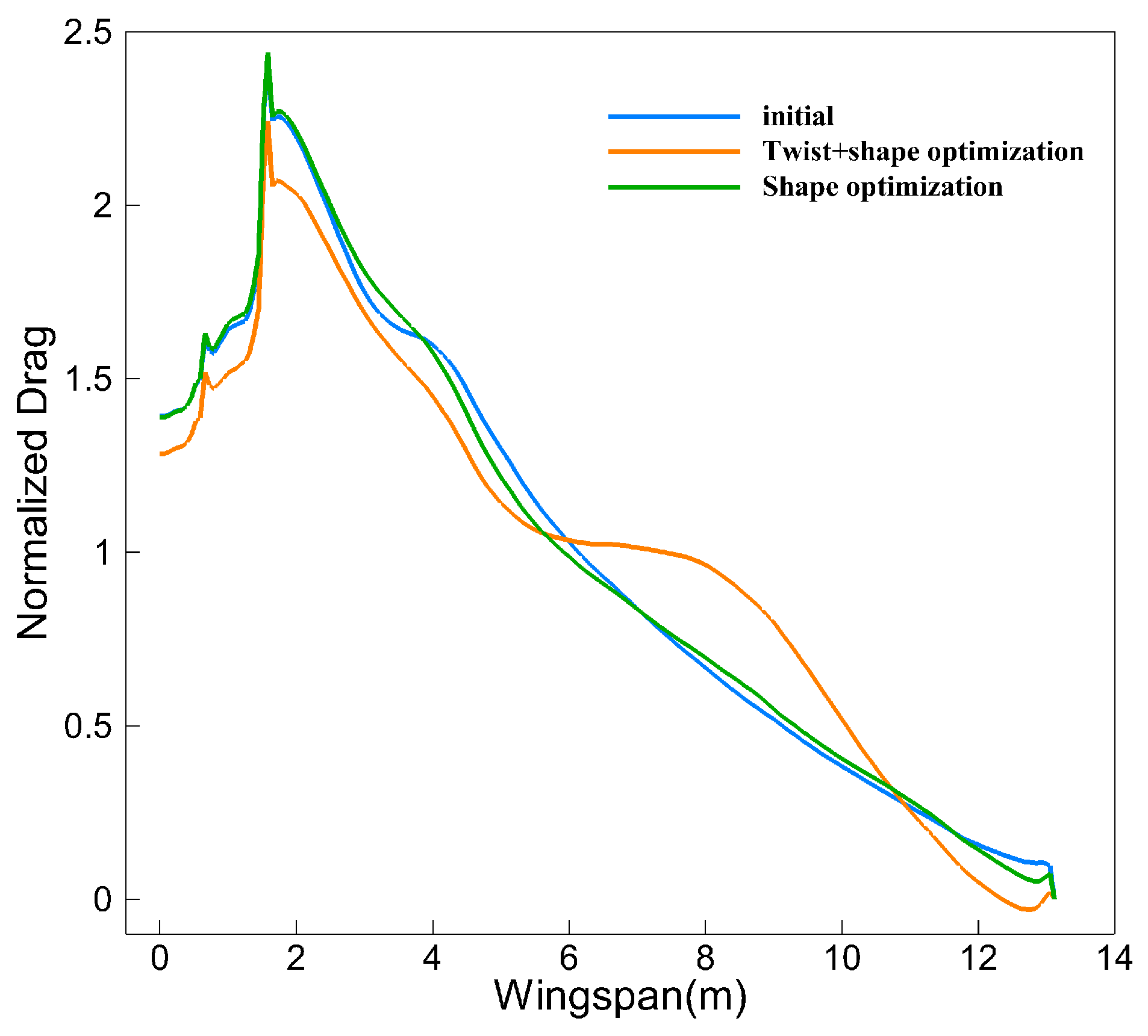
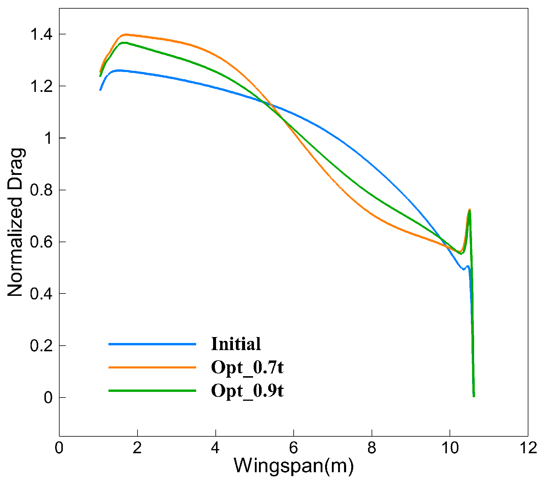
Figure 28 shows the distribution of normalized drag along the span direction before and after optimization. Compared with the initial configuration, the drag change trend of Opt_0.7t and Opt_0.9t is the same. The drag decreases in the range of 40–90% semi-span and increases in the range of 10% semi-spans of the wingtip. For a supersonic airliner, the volume wave drag is closely related to the thickness of the wing. Therefore, compared with the Opt_0.9t optimized configuration, the Opt_0.7t optimized configuration further reduces the thickness of the outer wing section, which further reduces the volume wave drag, and finally obtains greater drag reduction.
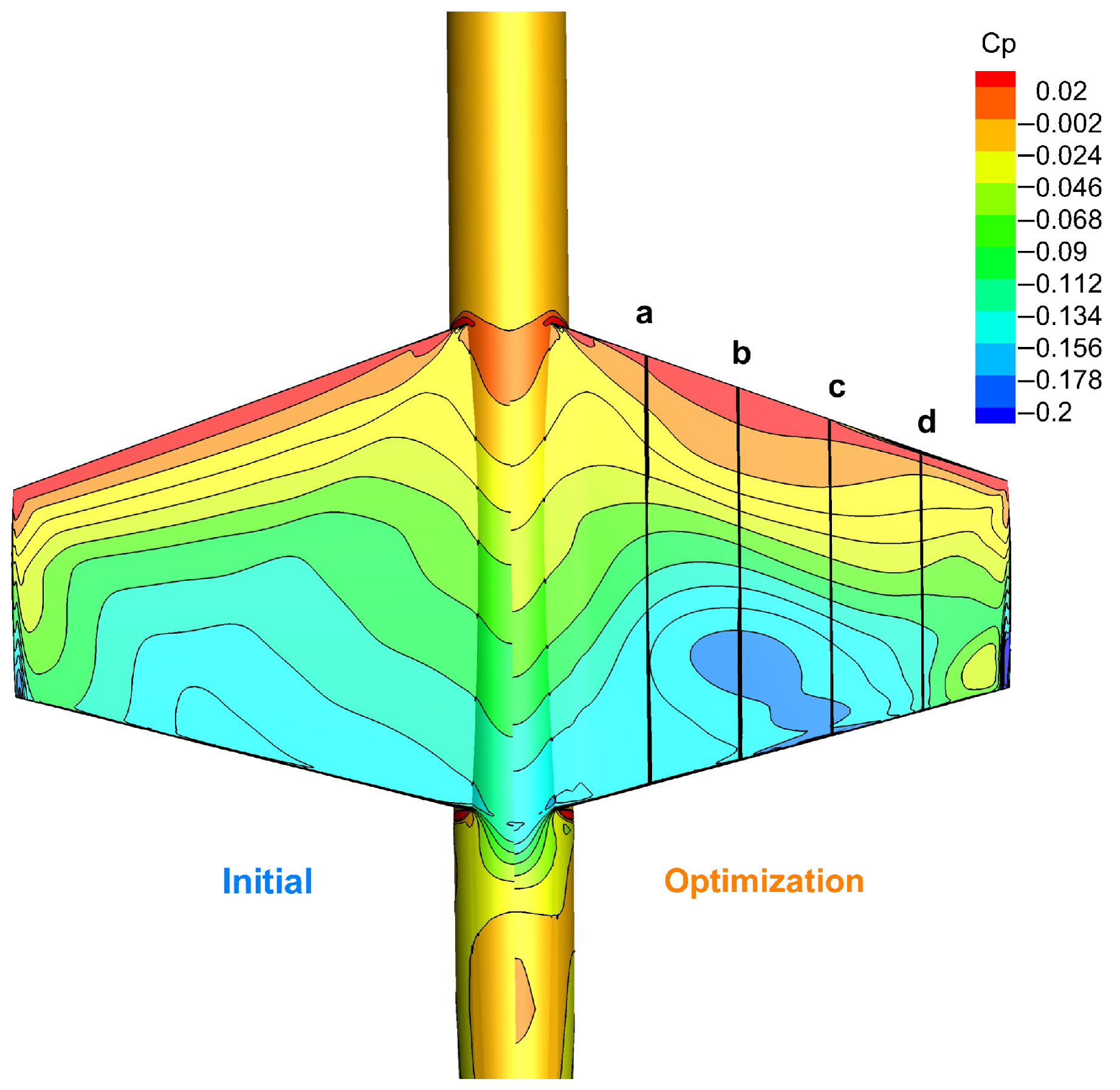
The contour of the pressure coefficient on the upper surface of the wing with the optimized configuration and the initial configuration is shown in Figure 29. Corresponding to Figure 30, a–d represents the slices in spanwise direction, respectively . The pressure distribution and airfoil comparison of a typical section is shown in Figure 30.
According to Figure 30a,b, in the inner wing section, compared with the initial configuration, the optimized configuration reduces the thickness of the leading and trailing edges, which is conducive to weakening the shock wave strength at the leading edge and reducing wave drag. At the same time, the thickness of the airfoil increases at , and the position of the maximum thickness is delayed.
Comparing the airfoil before and after optimization in Figure 30c,d, it can be found that in the outer wing section, the thickness of the optimized airfoil is smaller than that of the initial airfoil in the entire chord length range. Corresponding to the change in the spanwise distribution of normalized drag in Figure 28, the reduction in the airfoil thickness of the middle and outer wing sections reduces the drag. Although the drag of the inner wing may increase because of the larger thickness to satisfy the volume constraint, it is beneficial to the improvement of the overall drag performance.
The spatial distribution of the pressure coefficient and Mach number at the 50% and 90% of the wing span before and after optimization is shown in Figure 31. The results show that there are obvious differences, mainly on the lower surface of the leading edge on the wing, and each section presents the same change trend. After optimization, the pressure coefficient of the leading edge of each section after the shock wave is significantly reduced, and the Mach number after the wave is obviously increased. Therefore, the optimized configuration weakens the shock wave intensity at the leading edge of the wing and effectively reduces the shock wave drag.
For the purpose of qualitatively analyzing the trade-offs between lift and drag, as well as airfoil deformation and constraints in aerodynamic optimization design, sensitivity analysis is performed using gradient information obtained from the discrete adjoint equation for the initial configuration.
The derivative distribution of the lift/drag coefficient on the upper and lower surfaces of the wing with respect to the z displacement of the surface grid points in the initial configuration is shown in Figure 32, where the displacement direction is positive along the positive direction of the coordinate axis. For the supersonic leading edge configuration, when the lower surface deforms along the z axis, it has a greater influence on the lift/drag coefficient than the upper surface. Compared with the lift coefficient, the drag coefficient is more sensitive to the z displacement of the upper and lower surface.
The comparison of the airfoils before and after optimization (Figure 30) shows that, compared with the initial configuration, the upper and lower surfaces of the optimized configuration both move in a large range along the positive direction of the z axis. Combined with the sensitivity analysis results, when the lower surface moves in the positive direction of the z axis, the drag coefficient decreases accordingly, and the drag reduction effect is more significant. On the one hand, this deformation trend increases the lift coefficient in the dark red area of the sensitivity contour figure. On the other hand, reducing drag is the dominant direction of optimization since the lift can be maintained to meet the constraint through the deformation of the local profile. According to the results of sensitivity analysis, the movement of the upper surface of the wing along the negative direction of the z axis reduces the drag coefficient, but the actual optimization results show a contrary deformation. The reason is that the drag coefficient is more sensitive to the deformation of the lower surface than to the deformation of the upper surface. On balance, the optimizer mainly focuses on the lower surface deformation, and the upper surface moves accordingly to make sure that the final optimization configuration satisfies the thickness and volume constraints.
The convergence process of the optimized supersonic leading edge configuration is shown in Figure 33. After 35 main iterations, the constraints and the convergence conditions of the objective function are satisfied. From the convergence process of the main iteration, we can obtain the same conclusion as in subsonic leading edge optimization that the drag coefficient is reduced quickly in the first 10 main iterations of the gradient-based optimization.
The intermediate process of the airfoil at the typical sections of the inner wing 40% section and the outer wing 90% section from the initial configuration to the final optimized configuration is given, respectively. First, the comparison chart of P1 and P0 shows that in the beginning stage of the optimization, the changing trend of the inner and outer airfoils is the same, and the shock wave strength is weakened by reducing the thickness of the leading and trailing edges, while the camber of the airfoil increases, and the position of the maximum thickness moves backward. Compared with P1, the airfoil thickness of the inner and outer wing sections of P2 is reduced in a larger range near the leading and trailing edges, and the position of the maximum thickness is further moved back. Furthermore, the thickness of the airfoil of the outer wing section of P3 is reduced in the entire chord length range, while the thickness of the airfoil of the inner wing section is mainly increased in the middle section. The main reason for this phenomenon is that, considering the combined effect of the drag reduction objective and constraints, the optimizer increases the thickness of the inner wing section in exchange for a reduction in the thickness of the outer wing section and an overall greater drag reduction benefit. In the final stage of optimization, P4 has minor changes compared to P3, mainly to make small adjustments to the airfoil shape to make it smoother.
6. Conclusions
In this paper, the aerodynamic optimization design of supersonic wings was carried out by using the optimization design method based on discrete adjoint theory. The aerodynamic drag reduction principle and aerodynamic design characteristics of subsonic leading edge supersonic wing and supersonic leading edge supersonic wing are explored.
Aiming at the supersonic wing with a subsonic leading edge, the aerodynamic drag reduction single-point optimization design was carried out in the cruising state. Compared with the initial configuration, the optimized configuration with or without twist variables obtained 3.78% and 2.53% drag reduction, respectively. The optimized design mainly achieved the lift unloading of the inner wing section, the lift loading of the outer wing section, and the forward movement of the lift load by adjusting the geometric twist and increasing the airfoil camber, so that the wing load was closer to the elliptical lift distribution, thereby effectively reducing the induced drag without making a noticeable deterioration on pitching moment.
For the supersonic wing with a supersonic leading edge, compared with the initial configuration, the optimized configuration with the thickness constraints of and obtained drag reduction gains of 4.53% and 3.51%, respectively. Different from the optimized direction of the configuration with a subsonic leading edge, for the configuration with a supersonic leading edge, the wing load was transferred from the middle section to the wing root and wing tip through the geometric twist. Although the lift distribution deviated from the elliptical distribution, the optimized configuration significantly weakened the shock wave intensity. In other words, shock wave drag became the main contradiction in the design of this kind of configuration, rather than induced drag.
The analysis of the sensitivity contour and optimization results was conducted to show the difference between the two configuration optimization directions. The upper surface was particularly important for the design of the subsonic leading edge configurations; although, for the supersonic leading edge configuration, the lower surface dominated the lift and drag coefficients. For the trade-off between lift and drag, the drag coefficient of the two configurations was more affected by the deformation of the wing than the lift coefficient, so the optimizer treated reducing the drag as the dominant direction of optimization, and guaranteed lift constraints with the local deformation.
In this paper, the research on two kinds of supersonic wings shows that the optimization method can effectively improve the aerodynamic performance of the supersonic wing. The sensitivity results based on the discrete adjoint can qualitatively analyze the trade-off between aerodynamic force and airfoil deformation and constraint and can be used to guide the design of the future supersonic wings. Indeed, there is a conflict between the performance of supersonic wings at high speed and low speed, which requires further consideration of multi-point wide-speed domain aerodynamic optimization design. Meanwhile, simply considering the optimal design of aerodynamics cannot meet the needs of actual engineering. From the results of this paper, an increase in outer wing loads, which is beneficial to drag reduction, causes an increase in wing root bending moment that results in an increase in structural weight. An increase in the overall mass of the aircraft might negate the aerodynamic drag reduction. Therefore, a multidiscipline optimization design is necessary.
Author Contributions
Conceptualization, H.R., Y.S., J.B., Y.C., T.Y. and J.L.; methodology, Y.S., J.B. and J.L.; software, Y.C.; validation, H.R., Y.C., T.Y. and J.L.; formal analysis, H.R., Y.S., J.B., Y.C., T.Y. and J.L.; investigation, H.R., Y.S., J.B., Y.C., T.Y. and J.L.; resources, Y.S., J.B., T.Y. and J.L.; data curation, H.R., Y.S., J.B., Y.C., T.Y. and J.L.; writing—original draft preparation, H.R., Y.S., J.B., Y.C., T.Y. and J.L.; writing—review and editing, H.R., Y.S., J.B., Y.C., T.Y. and J.L.; visualization, H.R. and Y.C.; supervision, Y.S., J.B. and, J.L.; project administration, Y.S., T.Y. and J.B. All authors have read and agreed to the published version of the manuscript.
Funding
This research was funded by National Natural Science Foundation of China grant number 12002284.
Data Availability Statement
The data that support the findings of this study are available from the corresponding author upon reasonable request.
Conflicts of Interest
The authors declare that they have no known competing financial interests or personal relationships that could have appeared to influence the work reported in this paper.
References
- Han, Z.; Qiao, J.; Ding, Y.; Wang, G.; Song, B.; Song, W. Key technologies for next-generation environmentally-friendly supersonic transport aircraft: A review of recent progress. Acta Aerodyn. 2019, 37, 620–635. (In Chinese) [Google Scholar]
- Ang, H. General layout design analysis of large aircraft. Aviat. Manuf. Technol. 2009, 52, 40–43. (In Chinese) [Google Scholar]
- Gao, P. Civil aircraft design reference model Tu-144 supersonic transport aircraft. Civ. Aircr. Des. Res. 2015, 4. (In Chinese) [Google Scholar] [CrossRef]
- Sun, Y.; Smith, H. Review and prospect of supersonic business jet design. Prog. Aerosp. Sci. 2017, 90, 12–38. [Google Scholar] [CrossRef]
- Pietremont, N.; Deremaux, Y. Executive Public Summary of the Three Preliminary Aircraft Configuration Families; HISAC Publishable Activity Report; HISAC: Ormond Beach, FL, USA, 2005. [Google Scholar]
- Hanai, T.; Yoshida, K.; Usuki, K.; Tamaki, T. Research trend in supersonic transport. J. Jpn. Soc. Aeronaut. Space Sci. 1989, 37, 1–13. [Google Scholar]
- Chen, L.; Yang, X. Research progress and development trend of American supersonic business jet. Aeronaut. Sci. Technol. 2014, 11–15. (In Chinese) [Google Scholar] [CrossRef]
- Jameson, A. Advances in aerodynamic shape optimization. In Computational Fluid Dynamics 2004; Springer: Berlin/Heidelberg, Germany, 2006; pp. 687–698. [Google Scholar]
- Wu, H.; Da, X.; Wang, D.; Huang, X. Multi-Row Turbomachinery Aerodynamic Design Optimization by an Efficient and Accurate Discrete Adjoint Solver. Aerospace 2023, 10, 106. [Google Scholar] [CrossRef]
- Semlitsch, B.; Huscava, A. Shape Optimisation of Turbomachinery Components. In Proceedings of the 8th European Congress on Computational Methods in Applied Sciences and Engineering-ECCOMAS Congress 2022, Oslo, Norway, 5–9 June 2022. [Google Scholar]
- Rao, H.; Chen, Y.; Shi, Y.; Yang, T.; Liu, H. Adjoint-Based Aerodynamic Design Optimization and Drag Reduction Analysis of a Military Transport Aircraft Afterbody. Aerospace 2023, 10, 331. [Google Scholar] [CrossRef]
- Lyu, Z.; Xu, Z.; Martins, J. Benchmarking optimization algorithms for wing aerodynamic design optimization. In Proceedings of the Proceedings of the 8th International Conference on Computational Fluid Dynamics, Chengdu, China, 14–18 July 2014; Volume 11, p. 585. [Google Scholar]
- Mader, C.A.; Martins, J.R.; Alonso, J.J.; Van Der Weide, E. ADjoint: An approach for the rapid development of discrete adjoint solvers. AIAA J. 2008, 46, 863–873. [Google Scholar] [CrossRef]
- Marta, A.; Mader, C.; Martins, J.; Van der Weide, E.; Alonso, J. A methodology for the development of discrete adjoint solvers using automatic differentiation tools. Int. J. Comput. Fluid Dyn. 2007, 21, 307–327. [Google Scholar] [CrossRef]
- Chan, M.K.Y. Supersonic Aircraft Optimization for Minimizing Drag and Sonic Boom; Stanford University: Stanford, CA, USA, 2003. [Google Scholar]
- Choi, S.; Alonso, J.J.; Kroo, I.M.; Wintzer, M. Multifidelity design optimization of low-boom supersonic jets. J. Aircr. 2008, 45, 106–118. [Google Scholar] [CrossRef]
- Kirz, J. Surrogate-Based Low-Boom Low-Drag Nose Design for the JAXA S4 Supersonic Airliner. In Proceedings of the AIAA SCITECH 2022 Forum, San Diego, CA, USA, 3–7 January 2022; p. 0706. [Google Scholar]
- Kiyici, F.; Aradag, S. Design and optimization of a supersonic business jet. In Proceedings of the 22nd AIAA Computational Fluid Dynamics Conference, Dallas, TX, USA, 22–26 June 2015; p. 3064. [Google Scholar]
- Li, L.; Bai, J.; Guo, T.; Fu, Z.; Chen, S. Aerodynamic optimization design of supersonic airliner wing based on adjoint method. J. Northwestern Polytech. Univ. 2017, 35, 843–849. (In Chinese) [Google Scholar]
- Liu, S.; Bai, J.; Yu, P.; Chen, B.; Zhou, B. Aerodynamic optimization design of supersonic airliner considering sonic boom characteristics. J. Northwestern Polytech. Univ. 2020, 38, 271. (In Chinese) [Google Scholar] [CrossRef]
- Liu, B.; Hao, H.; Li, D.; Liang, Y. Adjoint optimization considering both aerodynamic and near-field sonic boom characteristics. Acta Aerodyn. Sin. 2022, 40, 1–11. (In Chinese) [Google Scholar]
- Seraj, S.; Martins, J.R. Aerodynamic Shape Optimization of a Supersonic Transport Considering Low-Speed Stability. In Proceedings of the AIAA Scitech 2022 Forum, San Diego, CA, USA, 3–7 January 2022; p. 2177. [Google Scholar]
- Bons, N.; Martins, J.R.; Mader, C.A.; McMullen, M.S.; Suen, M. High-fidelity aerostructural optimization studies of the Aerion AS2 supersonic business jet. In Proceedings of the AIAA Aviation 2020 Forum, Online, 15–19 June 2020; p. 3182. [Google Scholar]
- Morgenstern, J.; Norstrud, N.; Sokhey, J.; Martens, S.; Alonso, J.J. Advanced Concept Studies for Supersonic Commercial Transports Entering Service in the 2018 to 2020 Period; Technical Report; Lockheed Martin Corporation: Palmdale, CA, USA, 2013. [Google Scholar]
- Mangano, M.; Martins, J.R. Multipoint aerodynamic shape optimization for subsonic and supersonic regimes. J. Aircr. 2021, 58, 650–662. [Google Scholar] [CrossRef]
- Kenway, G.K.; Mader, C.A.; He, P.; Martins, J.R. Effective adjoint approaches for computational fluid dynamics. Prog. Aerosp. Sci. 2019, 110, 100542. [Google Scholar] [CrossRef]
- Spalart, P.; Allmaras, S. A one-equation turbulence model for aerodynamic flows. In Proceedings of the 30th Aerospace Sciences Meeting and Exhibit, Reno, NV, USA, 6–9 January 1992; p. 439. [Google Scholar] [CrossRef]
- Jameson, A.; Schmidt, W.; Turkel, E. Numerical solution of the Euler equations by finite volume methods using Runge Kutta time stepping schemes. In Proceedings of the 14th Fluid and Plasma Dynamics Conference, Palo Alto, CA, USA, 23–25 June 1981; p. 1259. [Google Scholar]
- Klopfer, G.; Hung, C.; Van der Wijngaart, R.; Onufer, J. A diagonalized diagonal dominant alternating direction implicit (D3ADI) scheme and subiteration correction. In Proceedings of the 29th AIAA, Fluid Dynamics Conference, Albuquerque, NM, USA, 15–18 June 1998; p. 2824. [Google Scholar]
- Biros, G.; Ghattas, O. Parallel Lagrange–Newton–Krylov–Schur methods for PDE-constrained optimization. Part I: The Krylov–Schur solver. SIAM J. Sci. Comput. 2005, 27, 687–713. [Google Scholar] [CrossRef]
- Knoll, D.A.; Keyes, D.E. Jacobian-free Newton–Krylov methods: A survey of approaches and applications. J. Comput. Phys. 2004, 193, 357–397. [Google Scholar] [CrossRef]
- Yildirim, A.; Kenway, G.K.; Mader, C.A.; Martins, J.R. A Jacobian-free approximate Newton–Krylov startup strategy for RANS simulations. J. Comput. Phys. 2019, 397, 108741. [Google Scholar] [CrossRef]
- Yoon, S.; Jameson, A. Lower-upper symmetric-Gauss-Seidel method for the Euler and Navier-Stokes equations. AIAA J. 1988, 26, 1025–1026. [Google Scholar] [CrossRef]
- Mayeur, J.; Dumont, A.; Destarac, D.; Gleize, V. Reynolds-averaged Navier–Stokes simulations on NACA0012 and ONERA-M6 wing with the ONERA elsA solver. AIAA J. 2016, 54, 2671–2687. [Google Scholar] [CrossRef]
- Jameson, A. Aerodynamic Shape Optimization Using the Adjoint Method; Von Karman Institute: Brussels, Belgium, 2003. [Google Scholar]
- Mavriplis, D.J. Discrete adjoint-based approach for optimization problems on three-dimensional unstructured meshes. AIAA J. 2007, 45, 741–750. [Google Scholar] [CrossRef]
- He, P.; Mader, C.A.; Martins, J.R.; Maki, K.J. An aerodynamic design optimization framework using a discrete adjoint approach with OpenFOAM. Comput. Fluids 2018, 168, 285–303. [Google Scholar] [CrossRef]
- Rashad, R.; Zingg, D.W. Aerodynamic shape optimization for natural laminar flow using a discrete-adjoint approach. AIAA J. 2016, 54, 3321–3337. [Google Scholar] [CrossRef]
- Shi, Y.; Mader, C.A.; He, S.; Halila, G.L.; Martins, J.R. Natural laminar-flow airfoil optimization design using a discrete adjoint approach. AIAA J. 2020, 58, 4702–4722. [Google Scholar] [CrossRef]
- Kenway, G.K.; Martins, J.R. Multipoint high-fidelity aerostructural optimization of a transport aircraft configuration. J. Aircr. 2014, 51, 144–160. [Google Scholar] [CrossRef]
- Albring, T.; Sagebaum, M.; Gauger, N.R. New Results in Numerical and Experimental Fluid Mechanics X: Contributions to the 19th STAB/DGLR Symposium Munich, Germany, 2014; Chapter A Consistent and Robust Discrete Adjoint Solver for the SU2 Framework—Validation and Application; Springer International Publishing: Cham, Switzerland, 2016; pp. 77–86. [Google Scholar] [CrossRef]
- Othmer, C. A continuous adjoint formulation for the computation of topological and surface sensitivities of ducted flows. Int. J. Numer. Methods Fluids 2008, 58, 861–877. [Google Scholar] [CrossRef]
- Andreoli, M.; Ales, J.; Désidéri, J.A. Free-Form-Deformation Parameterization for Multilevel 3D Shape Optimization in Aerodynamics. Ph.D. Thesis, Institute National de Recherche en Informatique et en Automatique, INRIA, Sophia Antipolis, France, 2003. [Google Scholar]
- Luke, E.; Collins, E.; Blades, E. A fast mesh deformation method using explicit interpolation. J. Comput. Phys. 2012, 231, 586–601. [Google Scholar] [CrossRef]
- Roache, P.J.; Ghia, K.N.; White, F.M. Editorial policy statement on the control of numerical accuracy. J. Fluids Eng. 1986, 108, 2. [Google Scholar] [CrossRef]
- Roache, P.J. A method for uniform reporting of grid refinement studies. ASME-Publ.-Fed 1993, 158, 109. [Google Scholar] [CrossRef]
Figure 1.
ONERA-M6 mesh convergence study.

Figure 2.
ONERA-M6 L2 mesh.

Figure 3.
Comparison of M6 wing calculation results with experimental data.

Figure 4.
Airfoil geometry and FFD control points.

Figure 5.
Optimization design system based on discrete adjoint for supersonic wing.

Figure 6.
LM1021 Model.

Figure 7.
Different mesh levels for subsonic leading edge configuration.

Figure 8.
LM1021 Mesh for optimization.

Figure 9.
FFD control frame for subsonic leading edge configuration.

Figure 10.
Thickness constraint for subsonic leading edge configuration.

Figure 11.
Different deformation forms of the FFD frame. (Orange points are after deformation and blue points are before deformation).
Figure 11.
Different deformation forms of the FFD frame. (Orange points are after deformation and blue points are before deformation).

Figure 12.
Comparison of the distribution of spanwise lift and twist angle before and after optimization for subsonic leading edge wing (‘Twist’ represents the geometric angle of the chord of the wing profile relative to the horizontal axis of the fuselage).
Figure 12.
Comparison of the distribution of spanwise lift and twist angle before and after optimization for subsonic leading edge wing (‘Twist’ represents the geometric angle of the chord of the wing profile relative to the horizontal axis of the fuselage).

Figure 13.
Comparison of spanwise drag distribution before and after optimization for subsonic leading edge wing.
Figure 13.
Comparison of spanwise drag distribution before and after optimization for subsonic leading edge wing.

Figure 14.
Comparison of pressure distribution of the upper surface before and after optimization for subsonic leading edge wing.
Figure 14.
Comparison of pressure distribution of the upper surface before and after optimization for subsonic leading edge wing.

Figure 15.
Comparison of pressure coefficients and airfoil before and after optimization for subsonic leading edge wing ( is the nondimensional spanwise percentage position, where y is spanwise coordinates and b is the span).
Figure 15.
Comparison of pressure coefficients and airfoil before and after optimization for subsonic leading edge wing ( is the nondimensional spanwise percentage position, where y is spanwise coordinates and b is the span).


Figure 16.
Comparison of pressure distribution of the upper surface before and after optimization.

Figure 17.
Comparison of pressure distribution and Mach number spatial distribution at 40% of the wingspan before and after optimization ( is the nondimensional spanwise percentage position, where y is spanwise coordinates and b is the span).
Figure 17.
Comparison of pressure distribution and Mach number spatial distribution at 40% of the wingspan before and after optimization ( is the nondimensional spanwise percentage position, where y is spanwise coordinates and b is the span).

Figure 18.
Derivatives of the upper (left) and lower (right) lift/drag coefficients with respect to the Z-axis displacement of the wing surface grid points for subsonic leading edge configuration.
Figure 18.
Derivatives of the upper (left) and lower (right) lift/drag coefficients with respect to the Z-axis displacement of the wing surface grid points for subsonic leading edge configuration.

Figure 19.
The optimization history of the subsonic leading edge configuration. Five typical steps were chosen to visualize the changing trend of pressure distribution during the optimization. The pressure distribution with different colors comes from the dot which has the same color in the function reduction line.

Figure 20.
Initial configuration with supersonic leading edge.

Figure 21.
Parameter definition of double-circular-arc supersonic airfoil.

Figure 22.
Blunted.

Figure 23.
Mesh of supersonic leading edge wing.

Figure 24.
Different mesh levels for supersonic leading edge configuration.

Figure 25.
FFD control frame for supersonic leading edge configuration.

Figure 26.
Thickness constraint of supersonic leading edge configuration.

Figure 27.
Comparison of the distribution of spanwise lift and twist angle before and after optimization for supersonic leading edge wing.
Figure 27.
Comparison of the distribution of spanwise lift and twist angle before and after optimization for supersonic leading edge wing.

Figure 28.
Comparison of spanwise drag distribution before and after optimization for supersonic leading edge wing.
Figure 28.
Comparison of spanwise drag distribution before and after optimization for supersonic leading edge wing.

Figure 29.
Comparison of pressure distribution of the upper surface before and after optimization for supersonic leading edge wing.
Figure 29.
Comparison of pressure distribution of the upper surface before and after optimization for supersonic leading edge wing.

Figure 30.
Comparison of airfoil and pressure coefficients before and after optimization for supersonic leading edge wing ( is the nondimensional spanwise percentage position, where y is spanwise coordinates and b is the span).
Figure 30.
Comparison of airfoil and pressure coefficients before and after optimization for supersonic leading edge wing ( is the nondimensional spanwise percentage position, where y is spanwise coordinates and b is the span).

Figure 31.
Comparison of pressure distribution of the upper surface before and after optimization ( is the nondimensional spanwise percentage position, where y is spanwise coordinates and b is the span).
Figure 31.
Comparison of pressure distribution of the upper surface before and after optimization ( is the nondimensional spanwise percentage position, where y is spanwise coordinates and b is the span).


Figure 32.
Derivatives of the upper (left) and lower (right) lift/drag coefficients with respect to the Z-axis displacement of the wing surface grid points for supersonic leading edge configuration.
Figure 32.
Derivatives of the upper (left) and lower (right) lift/drag coefficients with respect to the Z-axis displacement of the wing surface grid points for supersonic leading edge configuration.

Figure 33.
The optimization history of the supersonic leading edge configuration. Four typical steps were chosen to visualize the changing trend of pressure distribution during the optimization. The pressure distribution with different colors comes from the dot which has the same color in the function reduction line.


Table 1.
Gradient verification of lift coefficients with respect to design variables. (Underlines show the different significant numbers betweent the result from finite difference and adjoint method).
Table 1.
Gradient verification of lift coefficients with respect to design variables. (Underlines show the different significant numbers betweent the result from finite difference and adjoint method).
| Var | Finite Difference | Adjoint Equation | Rel. Error | |
|---|---|---|---|---|
| 4 | 0.0024191310 | 0.0024183648 | ||
| 6 | 0.0018757146 | 0.0018757950 | ||
| 9 | 0.0008184027 | 0.0008184097 | ||
| 16 | −0.0007589824 | −0.0007589494 | ||
| 20 | −0.0018793665 | −0.0018790061 |
Table 2.
Gradient verification of drag coefficients with respect to design variables. (Underlines show the different significant numbers betweent the result from finite difference and adjoint method).
Table 2.
Gradient verification of drag coefficients with respect to design variables. (Underlines show the different significant numbers betweent the result from finite difference and adjoint method).
| Var | Finite Difference | Adjoint Equation | Rel. Error | |
|---|---|---|---|---|
| 4 | −0.0466292505 | −0.0466005468 | ||
| 6 | −0.0361944061 | −0.0361960611 | ||
| 9 | −0.0157922613 | −0.0157923472 | ||
| 16 | 0.0146452139 | 0.0146445737 | ||
| 20 | 0.0362649685 | 0.0362579965 |
Table 3.
Geometric parameters of initial configuration.
| Parameters | Value |
|---|---|
| Length of fuselage (m) | 70.1 |
| Semi-span (m) | 12.8 |
| Reference semi-area () | 153.2 |
| Average aerodynamic chord length (m) | 21.0 |
| Sweep angle of inner wing section () | 78 |
| Sweep angle of outer wing section () | 69 |
Table 4.
Grid convergence study of subsonic leading edge configuration.
| Grid Level | Grid Size (Million) | (Counts) | GCI/% | Order p |
|---|---|---|---|---|
| L2 | 1.3 | 160.88 | / | |
| L1 | 5.3 | 152.87 | 1.488 | |
| L0.5 | 22.6 | 151.39 | 0.266 | 3.57 |
Table 5.
Optimization problem statement for subsonic leading edge configuration.
| Category | Name | Quantity |
|---|---|---|
| Objective | min | 1 |
| Design Variables | Shape | 240 |
| Twist | 5 | |
| AoA | 1 | |
| Constraints | = 0.142 | 1 |
| 1 | ||
| 1 | ||
| 1 |
Table 6.
Comparison of aerodynamic coefficients between the optimized configuration and the initial configuration for subsonic leading edge wing.
Table 6.
Comparison of aerodynamic coefficients between the optimized configuration and the initial configuration for subsonic leading edge wing.
| Configuration | (Counts) | (Counts) | (Counts) | AoA (Degree) | |||
|---|---|---|---|---|---|---|---|
| Initial | 0.142 | 152.87 | / | 86.88 | 66.00 | 2.15 | 0.0039 |
| Twist + Shape | 0.142 | 147.09 | −5.78 | 81.32 | 65.77 | 1.85 | 0.0040 |
| Shape | 0.142 | 149.00 | −3.87 | 83.06 | 65.94 | 2.04 | 0.0040 |
Table 7.
Geometrical parameters of the initial configuration with supersonic leading edge.
| Parameters | Value |
|---|---|
| Length of fuselage (m) | 48.7 |
| Semi-span(m) | 10.5 |
| Reference semi-area () | 71.4 |
| Aspect ratio | 2.6 |
| Average aerodynamic chord length (m) | 7.8 |
| Chord length of wing root | 10.4 |
| Chord length of wing tip | 4.4 |
| Sweep angle of leading edge () | 19.7 |
Table 8.
Grid convergence study of supersonic leading edge configuration.
| Grid Level | Grid Size (Million) | (Counts) | GCI/% | Order p |
|---|---|---|---|---|
| L2 | 3.0 | 289.56 | / | |
| L1 | 6.5 | 288.01 | 0.870 | |
| L0.5 | 14.0 | 287.13 | 0.487 | 2.27 |
Table 9.
Optimization problem statement for supersonic leading edge configuration.
| Category | Name | Quantity |
|---|---|---|
| Objective | min | 1 |
| Design Variables | Shape | 120 |
| Twist | 3 | |
| AoA | 1 | |
| Constraints | = 0.195 | 1 |
| 1 | ||
| 1 | ||
| 1 |
Table 10.
Comparison of aerodynamic coefficients between the optimized configuration and the initial configuration for supersonic leading edge wing.
Table 10.
Comparison of aerodynamic coefficients between the optimized configuration and the initial configuration for supersonic leading edge wing.
| Configuration | (Counts) | (Counts) | (Counts) | AoA (Degree) | |||
|---|---|---|---|---|---|---|---|
| Initial | 0.195 | 288.01 | / | 211.46 | 76.55 | 2.97 | 0.03 |
| Opt_0.7t | 0.195 | 274.97 | −13.04 | 198.30 | 76.67 | 3.00 | 0.02 |
| Opt_0.9t | 0.195 | 277.91 | −10.10 | 201.26 | 76.65 | 2.98 | 0.02 |
Disclaimer/Publisher’s Note: The statements, opinions and data contained in all publications are solely those of the individual author(s) and contributor(s) and not of MDPI and/or the editor(s). MDPI and/or the editor(s) disclaim responsibility for any injury to people or property resulting from any ideas, methods, instructions or products referred to in the content. |
© 2023 by the authors. Licensee MDPI, Basel, Switzerland. This article is an open access article distributed under the terms and conditions of the Creative Commons Attribution (CC BY) license (https://creativecommons.org/licenses/by/4.0/).
Share and Cite
MDPI and ACS Style
Rao, H.; Shi, Y.; Bai, J.; Chen, Y.; Yang, T.; Li, J. Aerodynamic Optimization Design of Supersonic Wing Based on Discrete Adjoint. Aerospace 2023, 10, 420. https://doi.org/10.3390/aerospace10050420
AMA Style
Rao H, Shi Y, Bai J, Chen Y, Yang T, Li J. Aerodynamic Optimization Design of Supersonic Wing Based on Discrete Adjoint. Aerospace. 2023; 10(5):420. https://doi.org/10.3390/aerospace10050420
Chicago/Turabian StyleRao, Hanyue, Yayun Shi, Junqiang Bai, Yifu Chen, Tihao Yang, and Junfu Li. 2023. "Aerodynamic Optimization Design of Supersonic Wing Based on Discrete Adjoint" Aerospace 10, no. 5: 420. https://doi.org/10.3390/aerospace10050420
Note that from the first issue of 2016, this journal uses article numbers instead of page numbers. See further details here.