1. Introduction
Airports play a significant role in regional economic growth and connectivity by providing the infrastructures that serve as nodes for air transportation services. Despite the COVID-19 pandemic’s recent drop in traffic growth, airports have handled a growing number of operations throughout the years [
1]. Nevertheless, existing infrastructure and current operating processes limit airport throughput. This indicates that airports have a restricted capacity [
2]. When expected demand approaches the available capacity, operational congestion arises. Therefore, the potential mismatch between limited airport capacity and growing demand has unfavorable effects [
3]. Access policies determine the outcomes of this possible situation. On the one hand, slot constraints can result in demand losses and/or demand displacement (e.g., to less desired times of the day or to other airports) in airports where access is regulated and capacity is coordinated (e.g., most of the busiest European airports) [
4]. On the other hand, the end effect may be over-capacity scheduling and delays, along with considerable congestion costs, in airports with primarily unrestricted access (e.g., most of the United States’ airports) [
4,
5].
Airport operators can take either supply side or demand-side actions to address the congestion issue [
4,
6,
7]. When looking for strategies to correct the imbalances between capacity and demand, these actions can be divided into three broad categories [
2,
4]: (i) demand management, (ii) infrastructure expansion, and (iii) operational improvements. Although these three interventions are interdependent, they can also be complementary, and typically follow a progressive sequence in which airports first plan their capacity based on demand forecasts, then they optimize operational procedures (on-ground handling and air traffic processes) to maximize capacity and reduce operating costs, and finally they tactically implement demand management schemes if capacity cannot meet airline demand with a certain level of service [
3,
8]. Lastly, in the long run, new capacity developments might be required to meet rising demand [
9].
Investments in Air Traffic Management (ATM) infrastructures mainly affect airside operations and are generally perceived as an intermediate solution between ‘soft’ measures (improvement of operational procedures) and ‘hard’ management of airport facilities (expansion of terminals, runways, and aprons) [
2]. In this sense, these investments include operational enhancements to improve the efficiency, reliability, and sustainability of airport operations. Therefore, they help increase capacity while limiting the impact on the airport infrastructure itself, offering more flexible solutions than traditional expansions of facilities [
10]. However, capacity adjustment poses challenges for airport planners and introduces a complex dynamic behavior of development and investment. It also highlights the problem of the risk aversion of airport operators and regulators and, more generally, the problem of how expectations are formed regarding the likely investment return [
11]. This creates a demand for valuation methods regarding investments in ATM infrastructures.
There are different economic approaches to the capacity expansion problem [
1]. One of the most extended techniques, due to its proven applicability and consolidated methodology, is Cost–Benefit Analysis (CBA). CBA is a systematic tool for calculating the benefits of a decision (often whether to develop a project or not) less the costs related to doing so. CBA allows us to consider externalities such as environmental consequences, regional connectivity, and even intangible effects such as customer satisfaction [
12,
13]. Identifying and measuring benefits and costs (including externalities) during the course of a project is necessary for the economic justification of investment decisions linked to the development of ATM infrastructures. This raises a number of economic challenges, including figuring out the project’s net present value of future flows of benefits and costs, developing feasible project alternatives, examining market institutional limits, and understanding governmental, airport, and airline policies [
10]. Airport investments have positive economic effects on congestion relief, passenger comfort, reduction in access and waiting times, avoidance of traffic diverting to competing airports or other modes of transportation, lower operating costs, enhancements to service predictability and reliability, and traffic growth (deviated and generated). These effects need to be properly evaluated and quantified.
According to neoclassical welfare economics, individuals make decisions that maximize their welfare. This neoclassical approach, which, in its most condensed form, assumes that people act rationally and are primarily motivated by self-interest, is the foundation for traditionally conducted airport capacity analyses, particularly CBA. However, these analyses must change to take into account more recent research in behavioral economics, which examines the psychological components of decision-making [
14,
15]. Particularly, the airport expansion problem should accommodate the most relevant behavioral challenges to conventional analyses: failure of the expected utility hypotheses, dependence of valuations on reference points, and time inconsistency [
14,
16]. Airport managers need methods to address these shortcomings.
Behavioral economics has developed primarily as a result of the greater inclusion of psychological research into models meant to explain or predict economic behavior [
14]. Beginning most notably with the work of Kahneman, Tversky, and Thaler in the late 1970s and early 1980s, behavioral economics challenges neoclassical economics, which frequently relies on von Neumann and Morgenstern’s mid-1940s formulation of expected utility theory. This theory assumes, as a model of decision-making under uncertainty, that individuals allocate utilities to outcomes and prefer the option that maximizes the expected value of this utility. Prospect theory [
17] and related models in behavioral economics reject this paradigm and suggest, in contrast, that preferences depend on the reference point from which they are measured (with losses valued more than gains and diminishing sensitivity with increasing distance from the reference point), and that probabilities are evaluated nonlinearly (with changes in probabilities near zero and crucial variations in intermediate probabilities). Additionally, traditional valuation methodologies such as Cost–Benefit Analysis (CBA), Net Present Value (NPV), and Internal Rate of Return (IRR) utilize increased discount rates to account for risk, providing a time bias effect that promotes short-termism [
18]. Consequently, the use of CBA, NPV, and IRR, which are markedly sensitive to the selection of discount rates, often discourages much-needed infrastructure projects that require large capital investments but yield positive cash flows slowly. Behavioral economics faces this inconsistency in time consideration by using non-exponential discount factors [
19].
In this paper, we are primarily concerned with the use of a behavioral approach to complete a traditional CBA for transportation projects. In particular, our objective is to develop a preliminary framework to determine preferences when evaluating the outcomes of ATM infrastructures in airports. To illustrate the applicability of this framework, we will apply it to a real case scenario: a CBA for evaluating the implementation of Automatic Dependent Surveillance–Broadcast (ADS–B), an investment aimed at improving ATM operational procedures in the airport environment. An aircraft can be tracked through the surveillance technology and electronic conspicuity device known as ADS–B, which uses satellite navigation or other sensors to establish an aircraft’s position and regularly transmits it [
20,
21]. Air traffic control ground stations can receive information as an alternative to secondary surveillance radar since the ground does not need an interrogation signal. In order to offer situational awareness and to allow self-separation, this ADS–B information can also be received by other aircraft [
22]. ADS–B is ‘automatic’ because neither the pilot nor external inputs are needed. As it depends on information from the aircraft’s navigation system, it is ‘dependent’. ADS–B is a cornerstone of both the NextGen program in the United States [
23] and the Single European Sky Air Traffic Management Research Project (SESAR) in Europe [
24]. The advantages of using ADS–B include greater flight efficiency, increased airspace and airport throughput, and enhanced operational predictability and flexibility [
25,
26]. Regarding airport operations, ADS–B, as a new air traffic control surveillance technology for traffic monitoring and information transfer, can be used as a means of tracking the movement of aircraft in the airport environment at a reduced cost: the key advantage is that it provides real-time information about the status of flights and the position of all aircraft within the airport and up to 350 nautical miles around it [
20]. It can also be used to perform post-operational analysis, allowing airport operators to discover the causes of congestion on the airport’s airside and surrounding airspace. The multiple benefits associated with the ADS–B system make it a technology that is being widely implemented in airports around the world. This has established a very extensive and continuously expanding ADS–B coverage. Since ADS–B is an investment aimed at improving ATM operational procedures and throughput, it represents an exceptional candidate for a CBA that evaluates the development of airport infrastructure. In this regard, the case study shows how the proposed novel framework for ATM investment evaluation could be used to better structure the capacity and demand management process in airports.
To adjust valuation methods and, particularly, CBA to behavioral challenges, our goal is to develop a preliminary framework that informs airport managers and policy makers in decision-making processes. We will derive insights on how investment and valuation assessments may be modified by the inclusion of deviations from the traditional model. The paper is structured as follows. In
Section 2, we begin by reviewing the current state of the research fields associated with our study: capacity and demand management, airport investment valuation, and behavioral economic challenges. This will place our findings in a broad context and highlight why they are important. In
Section 3, we present a traditional CBA for airport investments, particularly those aimed at airside infrastructures. This will serve as a basic valuation structure, setting its principles and standards.
Section 4 appraises behavioral economics inputs and how to incorporate them into the previous CBA methodology, achieving a new preliminary framework. In
Section 5,
Section 6 and
Section 7, we evaluate ADS–B as an investment for airport operations enhancement. This will provide us with a case study on investments in ATM infrastructures.
Section 8 provides the insights and findings of the study, particularly on how the new framework affects decision-making.
Section 9 concludes by offering the main results, recommendations, and limitations of the new framework.
Figure 1 illustrates the high-level methodological approach of the paper.
2. Background: How the Evaluation of Airside Investments Can Evolve from a Neoclassical to a Behavioral Approach
Although steady research has been carried out in the last two decades to solve the airport capacity and demand balancing problem [
27], congestion is far from over and is now more prevalent and getting severe. Furthermore, few attempts have been made to incorporate the challenges of behavioral economics in airport investment evaluations.
Several studies have detailed the main opportunities for addressing possible airport capacity and demand mismatches, including the timing and breadth of the available mechanisms (see [
4,
7,
27,
28] for a broad survey). Nonetheless, the literature has mainly focused on the effects of ‘soft’ approaches, which can reduce the cost of the solution but are intended for short- to medium-term implementation [
5,
6]. According to Ryerson and Woodburn [
29], airport operators may ignore or disregard demand management tools due to a variety of factors, including reduced impact and narrow scope, policy conflicts and uncertainty, long-term inefficiency, constrained economic development, and specific requirements for airline hub services (large airports pursue capacity expansions to enhance their ability to accommodate flights, remain hub airports, and provide intangible benefits to the communities they serve). Additionally, Fukui [
30] proved that demand management measures, such as slot allocation systems and congestion pricing plans, might occasionally be undermined by carriers’ hoarding tendencies. Due to these factors, airport managers can view capacity investments as preferable choices to meet rising demand while preserving a reasonable level of delay. ‘Hard’ approaches seek to boost potential capacity by altering the infrastructure itself, either with the construction of new alternative airports or with the extension of existing ones, typically by increasing the number of terminals or runways that are currently in use. These measures can result in substantial gains in capacity and, as a result, can directly address imbalances with demand.
Yet, recent infrastructure projects and past studies [
31,
32] have demonstrated that capacity additions are expensive, have a significant impact on the amount and nature of airport traffic, and are typically slow to accomplish. This usually entails a large time lag between expansion decisions and the final capacity deployment, a time lag that increases the inherent uncertainty of the development process since both traffic demand and the operational environment are subject to change. Decision-making procedures regarding capacity expansions are likely to be influenced by planning uncertainties, especially variability in traffic demand [
33], capacity dynamics and regularity [
34], as well as airport business models and airline competition [
31]. A comprehensive overview of uncertainties that affect the long-term planning of airports can be found in the Airport Cooperative Research Program (ACRP) Report 76 [
35]. In addition, airports are an integral part of the transportation network, where the consequences of delays and congestion can quickly spread throughout the system and affect a wide range of stakeholders. This increases the complexity, but also the need for expanding capacity. De Neufville and Odoni [
9] proposed the idea of dynamic strategic planning in airports to address risks and uncertainties during the expansion process. This approach aims to create adaptable solutions beyond standard what-if or sensitivity assessments. With the use of modular solutions, this concept evolved into dynamic adaptive planning [
36]. A more flexible approach to airport planning must be completed with a link between infrastructure development and airport business and consumer strategies [
37]. Airports are capital-intensive enterprises, as stated by Leucci [
37], and to manage the exposure on large capital expenditure programs more efficiently, airport managers must not only adopt flexible solutions and a step-by-step approach to capacity increase, but they also require novel evaluation methods that consider ‘real’ perceptions of risk and uncertainty.
Regarding the economic approach to airport capacity and demand management, it has evolved from mere documentation mechanisms to the process of assessing the value of additional passengers or additional capacity at an airport [
31,
38]. Now, the field must seek to qualify and quantify the main relationships and trade-offs between capacity, quality of service, and profitability [
38,
39], i.e., to understand the economic benefits of adding airport capacity. Due to the variable and uncertain nature of traffic demand and the nonlinear relationships between variables, the problem is particularly complex when determining the value of a marginal change in capacity for congested airports [
31]. As previously described, the main economic methods to assess capacity expansions (namely airport valuation, cost–benefit analysis, and capacity/demand balancing) are traditionally rooted in neoclassical welfare economics. Weimer [
16] concluded that it is necessary to complete the traditional theoretical approach with practical inputs that reflect the observed deviations from the neoclassical evaluation framework in ‘real’ performance. Based on this, and to better understand how and why people behave and make decisions the way they do in the ‘real world’, behavioral economics tries to introduce insights from other social sciences, particularly psychology, into traditional economic analyses and models. It challenges the idea of neoclassical economics that most people have clearly defined preferences and base their decisions in a well-informed and self-interested manner [
40]. Hence, behavioral economics can be recognized as the study of decisions that do not follow the neoclassical paradigm of people making decisions based on maximizing utility. According to empirical evidence, deviations from neoclassical assumptions tend to be consistent and systematic, which makes them predictable. Individual preferences are not necessarily compatible with coherent choices [
41]. Thus, applied welfare economics must seek a distinct framework for determining public trade-offs to be applied in the assessment of projects [
42]. Behavioral economics plays a growing role in policy evaluation and proposes many cognitive biases and limitations, raising doubts as to whether the revealed willingness to pay is equal to the true willingness to pay [
43]. Recognizing these limitations of the neoclassical approach, airport capacity and demand management, particularly the evaluation of airport infrastructure, should be completed with the most influential behavioral concepts in capacity expansion: risk perception and loss aversion, expected utility deviations, and time inconsistency [
19]. In particular, airport managers and policy makers could take advantage of new conceptual frameworks that complement traditional CBA with behavioral inputs.
Concerns about the implications of behavioral economics for CBA have generated three types of academic responses [
19]. First, some scholars consider revealed or stated preferences as an inappropriate basis for assessing the relative efficiency of alternative public policies, particularly in the context of the many behavioral challenges to the neoclassical paradigm. In this sense, Bronsteen et al. [
44] suggest replacing CBA with a wellbeing analysis based on surveys of people’s stated assessments of their own subjective happiness, while Brennan proposes abandoning CBA in favor of greater reliance on democratic delegation of authority to make decisions or produce regulations. A second type of intellectual response has been attempts to revise welfare economics, the conceptual foundation of CBA, so that it does not depend on assumptions that behavioral economics research often finds violated. For example, Sugden [
45], Bernheim and Rangel [
46], and Bernheim [
47] provide conceptually coherent behavioral alternatives to neoclassical welfare economics. Finally, a third academic response involves accommodating behavioral challenges within the existing CBA framework on a case-by-case basis. It means identifying relevant behavioral challenges in particular contexts, assessing their likely importance for both the prediction and evaluation of policy impacts, and adapting standard methods to accommodate in a consistent way. This was the approach taken by Robinson and Hammit [
14]. As the main goal of this paper is to provide a particular framework for CBA in the field of ATM investments in airports, this third approach appears to be the most useful response to provide guidance for the inclusion of behavioral challenges.
The main objectives of the study arise from the needs observed in the review of the literature review on the subject. The gaps we aim to fill are:
Propose a preliminary model for the CBA of investments in ATM infrastructures that evolves from the traditional approach to consider behavioral economics inputs.
Apply this model to a case study—a CBA for the implementation of ADS–B technology aimed at improving airport operations and increasing available capacity, thus reducing delays and alleviating congestion.
Obtain information on how investment decisions in airport airside facilities would be modified by including behavioral considerations.
Consequently, the purpose of our work is to highlight the most relevant challenges that behavioral economics presents for conventional analysis in order to develop a new framework. This framework aims to help decision-making processes associated with the problem of airport capacity expansion.
3. A Methodological Framework for Classic Cost–Benefit Analysis
The application of behavioral economics concepts will be implemented over a conventional Cost–Benefit Analysis (CBA) methodology for evaluating airport investments. We focus on CBA because it offers widely acknowledged concepts and principles, a solid formulation, a body of shared literature, and has demonstrated its applicability throughout time [
12,
48,
49]. It is one of the most widespread techniques for decision-making in policy plans, including transportation developments [
32,
50,
51]. CBA can generally be thought of as a methodology to calculate the efficiency of policy alternatives [
52].
A CBA of airport infrastructure can be structured using a systematic formulation based on a well-defined and reliable methodology [
32,
50,
51]. The fundamental tenet of this approach is that airport investments should be evaluated as upgrades to infrastructure intended to meet a demand for transportation. As a result, we should concentrate on appraising how the investment would affect the generalized cost of travel for users and identifying the costs related to the provision of the transportation service, including those associated with the airport and the airlines [
11].
Figure 2 summarizes the stages involved in the process of performing a CBA: in order to characterize the affected universe with and without the project or policy intervention and to evaluate the incremental costs and benefits, this analysis involves several iterative and connected steps [
14], which are depicted in the diagram. The first steps involve defining the framework of the analysis, i.e., a complete description of the conditions in the baseline scenario (step one) and in the scenario that results after the intervention (step two). It includes a prediction of the expected consequences of the policy or project that is being evaluated. Costs and benefits are later detected and categorized (steps three and four). Creating a timeline for anticipated costs and benefits throughout the life of a project is crucial to the decision-making and planning processes. These project costs and benefits (including externalities) are quantified in monetary terms and adjusted for the time value of money, thus providing present values (steps five and six). Finally, various decision criteria are applied to decide whether to launch the project or not (for example, an assessment of Benefit–Cost Ratio, NPV, or IRR).
The economic evaluation of airport projects raises issues that are common to every CBA of a major investment in transportation infrastructure. The comparison of benefits and costs (either social or financial), as well as measures and standards to avoid errors and biases, are not appreciably different: definition of the base case; identification and quantification of relevant effects (including externalities); use of appropriate assumptions and parameter values; and prevention of double or triple counting [
32].
The idea behind CBA is to evaluate the
NPV of the investment [
53].
Figure 3 shows the typical time-stream of a project’s net benefits [
12]. Investment costs in the initial years of a project’s life lead to net benefits being negative (costs exceed benefits). In the later stages, net benefits are positive (benefits exceed operating costs and capital replacement costs). We seek to evaluate if this time-stream of project values results in a positive net present value (
NPV > 0).
The
NPV of an investment in transportation infrastructure can be simplified to Equation (1) [
16], assuming that investment costs are realized in year 0 (or in the case of a larger period before year 0, converted into year 0 values) and changes in benefits and costs of the implemented project occur in year 1 onwards (replacement costs during the project’s life will also be converted to their present value):
where
I represent the investment costs (the initial capital costs and the present value of the replacement costs),
T is the project life, ∆
CSt is the change in consumer surplus in year
t, ∆
PSt is the change in producer surplus in year
t,
i is the discount rate (annualized rate of interest), and
is the discount factor (the factor by which any future cash flow should be multiplied to obtain its present value). The graphical representation of this model, with respect to the practical approach of the CBA, will be shown in Figure 15 (
Section 7).
The change in consumer surplus can be estimated with ‘the rule of a half’, as shown in Equation (2) and
Figure 4. The consumer surplus reflects the potential reduction in prices and the time-saving effects of the investment project.
with
, where
gt0 is the generalized cost in year
t without the investment;
gt1 is the generalized cost in year
t with the investment;
qt0 is the volume of airport users in year
t without the investment;
qt1 is the volume of airport users in year
t with the investment;
p is the price per trip including airport charges, airline ticket, and access and egress money costs; and
τ is the value of total trip time (flying, access, egress, and waiting).
The change in producer surplus (for any of the affected producers) is given by Equation (3). Changes in producer surplus require estimating incremental revenues and costs for the airport operator, airlines, and other companies directly affected by the project.
where
and
denote total variable costs without the project and with the project.
Equation (1) assumes that the discount factor for the investment follows the traditional exponential curve: , i.e., discount factors for future periods fall at an exponential rate tending to zero over time. By definition, the discount factor at present time (t = 0) is 1.0.
The economic benefits of investments in airport infrastructure can be ascertained through a decrease in resource costs if we assume competitive markets for airlines and other companies offering airport services. To exemplify these benefits, let us consider an airport project that reduces total travel time (
τ1 −
τ0) and assume that prices remain unchanged (
Section 7 presents a case of investment in ADS–B technology, which follows these assumptions). This kind of investment, which ultimately results in higher capacity [
11,
32], is illustrated in
Figure 5. The vertical axis measures the generalized costs of passengers and their willingness to pay for airport services, while the horizontal axis measures the number of passengers per unit of time. Curve
D represents demand conditions for air traffic at a period of time, and curve
C represents the cost to the average passenger.
The analysis proceeds by considering the demand for which the airport represents the preferred mode of transportation. As demand grows, the demand curve shifts to the right. Capacity in the initial situation corresponds to the pair (
qa,
g0), meaning that when the conditions faced by the airport are as described by curve
D0, a maximum of
qa passengers can be attended to over a period, at a constant generalized cost equal to
g0. The average generalized cost function
C implies that if the critical point
qa is reached, at this capacity level there can only be an increase in traffic at a higher average cost. According to this initial situation, demand in a period (
D0) has an imperfect substitute (e.g., another less convenient flight, airport, or mode of transportation) available at a generalized cost of
g1 that is higher than that of
g0. However, with demand
D0, all passengers willing to pay
g0 will be served. From that point onwards, further demand growth will cause congestion in the airport, creating time costs and delays, forcing passengers to travel at less preferred times if there are no investments in capacity. This is represented in
Figure 5 by curve
C, which provides a higher cost to the average passenger when demand grows. If the airport decides not to add capacity as demand increases, pushing the demand curve to the right, the airport throughput would exceed
qa, resulting in increased congestion. Eventually, congestion and the corresponding generalized cost to passengers would reach a level where the average passenger would not have a preference between using the airport or the alternative means of transportation. The intersection of curves
C and ‘Alternative’ represents this situation. At that moment, the generalized cost incurred by the average passenger would be
g1, which is the generalized cost to passengers (for whom the airport is the preferred mode of transit) of diverting to the alternative mode of transportation. Let us presume that the growth in demand in the following period
t leads to
Dt. Depending on which cost (
g0 or
g1) applies,
Dt would be fully served by the airport if the project is implemented (
qd), but would only be partially satisfied by the existing airport facilities if the project is not carried out (
qb). In the latter case, there will be some deviated traffic to the second-best alternative (
qc −
qb), and some ‘discouraged’ or deterred traffic
(qd −
qc) that cannot be attended to at these costs. The project leads to higher capacity, so the situation with the project is illustrated by the possibility of maintaining a generalized cost of
g0 as demand changes to
Dt (
qd). At a demand level equal to
Dt, without the project, the equilibrium point in the airport would be
qb <
qd. Therefore, the equilibrium level for demand
Dt with and without the project has been determined (
qd and
qb, respectively), and we can evaluate the economic benefit of the investment project.
Figure 5 identifies three categories of user benefits: (i) benefits to existing users (
qb); (ii) benefits from avoided diversion costs (
qc −
qb); and (iii) benefits from new generated traffic (
qd −
qc). These benefits can be measured as follows. The benefits to current users are given by (
g1 −
g0)·
qb, since the alternative travel option now determines the maximum number of passengers (
qb). The benefits from avoided diversion costs are given by (
g1 −
g0) · (
qc −
qb), since passengers in the portion (
qc −
qb) will deviate to a less desirable alternative. The diversion could be ‘in time’ if passengers are compelled to depart at less convenient times or ‘in mode’ if they must choose an alternative airport or mode of transportation. The ‘rule of a half’, as shown in Equation (2) and
Figure 4, applies equally to both diverted and generated traffic. The benefits of diverted traffic are given by the difference (
g1 −
g0) in
Figure 5. This amount should be understood as the average, which is equal to half of the time savings interval. The benefits from new generated traffic due to the project are given by 0.5·(
g1 −
g0)·(
qd −
qc). This benefit can also be read as the amount of deterred traffic that is avoided as a result of the investment, given a future demand prediction equal to
Dt. Note that additional benefits (taxes and revenues above incremental costs) may be linked to deviated and generated traffic.
This simplified analysis ignores three elements: first, the potential existence of administrative capacity rationing; second, the possibility that there could be different generalized costs for existing and deviated passengers; and finally, the possibility of insufficient capacity to meet demand during the project’s lifetime.
Figure 6 illustrates the framework for a project to expand the capacity of an airport, showing the distinct types of traffic with and without the project. The reduction in costs for passengers and firms could lead to an increase in traffic. This is what it is known as induced traffic, with two basic types: deviated and generated.
Changes in producer surplus, assuming a financial and economic approach, will entail the estimation of incremental benefits and costs for the airport, airlines, and other companies and communities directly affected by the project. Adopting a supply led model suggests that improving the transportation infrastructure or increasing the quality of the supply of transportation services in a region will automatically stimulate economic activity and boost local development. This might happen for a number of reasons [
54], including the widening of markets, greater production, and multiplier effects or indirect effects on employment in construction and operations.
Therefore, financial benefits derived from investment in ATM infrastructure, which mainly affects airside operations, correspond to the revenues obtained by the airport authority, airlines, and retail firms with commercial operations at the airport directly affected by the project. Investment on the airside will also produce two expected economic benefits (apart from the potential ability to manage more traffic):
First, an expansion in airside capacity will allow for an increase in both departure frequency and the number of routes available from the airport. This will reduce the frequency delay and perhaps even the duration of the trip, both of which help to lower the generalized cost of transportation. The frequency delay represents the difference between the preferred departure time for an average passenger and the closest actual flight departure that is acceptable to the passenger [
32]. Other things being equal, the higher the departure frequency, the lower the frequency delay, and, consequently, the time cost of travel for the passenger.
Second, airside investments might shorten the process time for aircraft, saving operating costs for airlines. These projects improve flight efficiency and, for instance, would reduce fuel consumption (internal benefit). The greater number of efficient procedures would, in some cases, enhance air transportation sustainability (external benefit) by lowering harmful emissions for the environment (reducing air pollution) or limiting noise in the airport vicinity.
Consequently, results derived from airside investments can be summarized into four categories: first, reductions in travel, access, and waiting time; second, improvements in service reliability and predictability; third, reduction in operating costs; and finally, increases in traffic.
5. Problem Statement: Investments in Air Traffic Management Infrastructures
The definition and specification of capacity is an essential issue when assessing investments in airport infrastructure. Due to its complex and dynamic nature, airport capacity is quite difficult to describe. It depends not only on the available infrastructure but also on operational processes and external factors. Anyway, we can understand capacity as the ability of an airport, or a part of it, to process entities (aircraft, passengers, luggage, goods, vehicles, etc.) over a certain period of time [
2,
55]. Airport capacity is commonly expressed in units such as passengers per year or operations per hour. Nevertheless, the implications of potential traffic congestion, required levels of service, and tolerable delays are not taken into account by this definition. Due to this particularity, rooted in the difference between infrastructural and operational capacity, the following two terms are typically used to characterize airport capacity: throughput and practical capacity [
9].
Throughput capacity is the maximum rate at which aircraft operations can be managed without accounting for any minor delays that can be caused by operational flaws or unforeseen random events. Meanwhile, practical capacity is the number of operations that can be handled over time with no more than a certain amount of delay. This introduces the concept of ‘level of service’, typically expressed through a threshold related to the maximum tolerable average delay. As practical capacity is defined in terms of delay while throughput capacity is not, this represents a significant difference between the two measures of capacity. In order to ensure airport users an acceptable level of service, such as an average daily flight delay of four minutes, airports operate and serve demand below their practical capacity. Therefore, although throughput capacity is the most accurate theoretical definition of capacity and the foundation for airport capacity planning [
65], practical or sustainable capacity should not be exceeded for extended periods in order to ensure a given level of service.
Figure 10a shows the theoretical relationship between capacity and delay, illustrating that delay does not appear only at the capacity limit.
Long before airport operations reach throughput capacity (leading to queueing), there will be some delay, and as demand rises, the amount of delay increases exponentially. As mentioned in
Section 1, congestion depicts a scenario in which demand surpasses capacity and normal operations are therefore hampered. Guidelines for congestion relief or mitigation through demand and capacity management are provided by this non-linear relationship between capacity and delay. Airport performance is particularly sensitive to even slight changes in airport capacity from a supply standpoint.
Figure 10b depicts an average distribution of aircraft delays at a given level of demand; in this example, data were collected during a busy day at a major European hub. It should be noted that most delays were low and that, despite the average delay being short (5 min), a small number of aircraft experienced quite lengthy delays of 15 min or more.
The capacity of the airport airside depends not only on the facilities, but also on their use. When increasing capacity by adding new facilities or by improving operational procedures, we can find two ‘limit’ situations. If the acceptable delay threshold is maintained, there is an increase in practical capacity. If expected demand is maintained, there is a reduction in average delay, which means a higher level of service is provided.
Figure 11 illustrates these situations: increasing capacity shifts the curve rightward, providing a new asymptotic value for throughput capacity. An investment in capacity usually brings an intermediate scenario where both effects can be registered: the practical capacity is increased (allowing the airport to manage more traffic), and the delay threshold is partially reduced.
For the purpose of our analysis, we consider ATM investments that imply a combination of both effects: (i) an expansion in practical capacity and, therefore, an increase in induced traffic brought by the higher aircraft movement capacity of the airport; and (ii) an improvement in the level of service reached by lower waiting times and reduced average delay. This is the case of investments in ADS–B technology, as appraised in
Section 7.
Three effects arise when an airport increases its aircraft movement capacity. First, it allows for potential growth in the capacity for handling passengers and cargo. Second, it provides a higher flight frequency, which benefits passengers by enabling increased departure time options. This greater choice results in frequency delay reductions, meaning that the time gap between the passengers’ preferred departure time and the closest available departure time is lowered [
66,
67,
68]. Third, the average size of the aircraft using the airport may vary as departure frequency increases. Larger aircraft are less costly to operate per seat than smaller aircraft [
69], so a change in aircraft size has a large effect on airline operating costs. Due to the indivisibilities of airport expansion, runway capacity cannot increase proportionally with traffic. As an airport manages more passengers, the runway will eventually have to handle larger aircraft.
When an airport increases its capacity for aircraft movement, two effects can produce reductions in the average size of aircraft [
70]. First, airlines would increase the frequency of flights in order to compete for time-sensitive business passengers, a tendency that would require using smaller aircraft [
71]. Second, there will be new airlines operating at the airport, typically using smaller aircraft when developing new routes. In the scenario without a project, when there is no increase in airside capacity, airlines will be forced to operate larger aircraft so that traffic growth can be accommodated. Consequently, the decision to invest in airside capacity will have to consider the possible trade-off between reduced frequency delay at a higher cost per seat (with project) and constant frequency delay at a lower cost per seat (without project).
Figure 12a illustrates the trade-off between aircraft size and departure frequency, considering both airlines and airports [
11,
32]. The marginal frequency delay (the cost associated with not having a departure flight available at the requested time), which decreases as the flight frequency grows, is shown by the downward-sloping frequency delay curve (
FD). The vertical axis on the left side measures the monetary value of the frequency delay (e.g., in Euros), and the vertical axis on the right side measures the inverse of the aircraft size (
AS). The departure frequency (
F) is measured along the horizontal axis. According to airline strategies,
FD varies directly with the average
AS, meaning that the larger the aircraft, the lower
F and the higher
FD for a given number of seats supplied. As a result, the
FD curve grows (or shrinks inversely) with
AS, as depicted by the vertical axis on the right side. The inverse relationship between
F and the generalized cost is indicated by the marginal
FD curve (negative slope). The
FD curve moves upward in response to an increase in the value of time. Assuming constant returns to scale when providing an enhancement of airside capacity, the marginal cost to the airport of adding an additional flight is represented by the horizontal
Ca curve. The total cost of providing the service, including both airport and airline costs, is characterized by the
C curve. The slope of the
C curve is positive because, for a given number of seats supplied, as
F increases, there is a reduction in
AS, implying higher costs per seat as smaller aircraft register larger unit costs [
69]. Hence, the
C curve reflects the direct relationship between
F and cost per seat regarding the vertical axis on the left side and the inverse relationship between
F and
AS regarding the vertical axis on the right side.
AS will have to grow as overall traffic increases for a certain level of
F, lowering the marginal cost per seat and rotating the
C curve clockwise, downwards. Note that in
Figure 12, traffic along the horizontal axis is not constant: increased
F generates traffic because it improves service quality and reduces
FD. This effect is taken into account by cost curve
C.
The departure frequency (
F) capacities of the system before and after the airside investment project are shown in
Figure 12a by the vertical ‘Movements 1’ and ‘Movements 2’ curves, respectively. According to the example in
Section 7, the ‘Movements 1’ curve represents the
F capacity of the airport without ADS–B, which is equal to
f1, and the ‘Movements 2’ curve represents the
F capacity when adding ADS–B technology, which is higher and equal to
f2. Therefore, the ‘Movement’ curves represent two levels of airside capacity, before and after equipment enhancement. When the airside capacity of the airport is given by ‘Movements 1’ and
F is limited at
f1 (point
a, and a capacity for aircraft movements of
f1), the vertical axis on the left side indicates that the marginal benefit of adding a departure frequency is
fd1. This value is higher than the marginal cost of decreasing
AS, given by
c1 (point
d). Expanding airside capacity to ‘Movements 2’ increases
F to
f2, which is accompanied by a decrease in
AS. This can be explained by the fact that in
f1 the passenger costs due to
FD are
fd1, higher than the marginal operating costs, which are equal to
c1. Then, the willingness of passengers to pay for an additional frequency is greater than the marginal cost associated with reducing
AS (
fd1 >
c1), and thus airlines have an incentive to increase
F, implying a decrease in
AS. Therefore, flight frequency increases to equilibrium at
f′ (point
b), resulting in a decrease in
AS. At this point
b, the marginal benefit of improving
FD is equal to the marginal cost of decreasing
AS (
fd′ =
c′). The benefit of expanding airside capacity from ‘Movements 1’ to Movements 2’, allowing for an increase in
F, is equal to the area ‘
abd’. There would be, at least initially, excess airside capacity (
f2 >
f′). The provision of facilities operating at less than full capacity is due to technological invisibility in production functions (although this may well be the welfare-maximizing option; traffic growth generally means that capacity is ultimately covered).
Therefore, an investment in ADS–B technology expands airport airside capacity and allows for an increase in flight frequency (reduction in frequency delay).
Time will bring about two effects: growth in traffic, shifting the
C curve downward, and increases in the value of time as income grows, shifting the
FD curve upward.
Figure 12b reflects the effects of the increasing incomes, which change the
FD curve from
FD′ to
FD″. This shifts the equilibrium level of frequency from
f′ to
f″. Frequency level
f′ is lower than the maximum capacity brought by the airside project, but frequency level
f″ would require an increase in airside capacity. Therefore, the higher income and accompanying higher value of time makes the case for airside investments even at the expense of higher operating costs resulting from operating smaller aircraft. The effects of time (
C curve moving downward and the
FD curve moving upward) would expand the ‘
abd’ area (benefit of expanding airside capacity) from its three corners, which means that the benefit of adding airside capacity increases over time. The economic returns from investing in airside capacity are given by the present value of the future stream of benefits determined by the ‘
abd’ area in each year during the life of the project and by the present value of the capital investment required for the added capacity. Until point b exceeds the capacity of ‘Movements 2’, there will be no benefit from an additional investment in airside capacity.
Variations in the
C curve can only be explained by external changes in traffic caused by technology, population, and income growth. In this regard,
Figure 12b also illustrates the effect of technology, which determines the shape of curve
C. Even though technology can be understood as a given input in the short and medium terms, improvements in technology may make aircraft more cost-effective in the long term, which would shift curve
C downward. This would support investing in airside capacity for any given amount of income and traffic, other factors being equal. In contrast, the
C curve would be shifted upward for any level of technology if there were an increase in fuel prices or polluting emissions, requiring less airside capacity for a given amount of income and traffic. Developments in aircraft technology are usually guided toward advances in fuel efficiency. Therefore, increasing income and advances in technology (curve
C moved downward) support the addition of airside capacity, whereas higher costs of energy and polluting emissions discourage investments in airside capacity (curve
C moved upward).
6. ADS–B as an Investment for Airport Operations Enhancement
Automatic Dependent Surveillance-Broadcast (ADS–B) is a surveillance technique that enables the tracking of aircraft by periodically broadcasting their location, which the aircraft itself determines using satellite navigation or other sensors. Thus, ADS–B combines a network of satellites, transmitters, and receivers to update air traffic controllers and flight crews on the position and velocity of nearby aircraft [
21]. Since ground-based interrogation signals are unnecessary, the data can be received by air traffic control ground stations as a replacement for secondary surveillance radar. To allow self-separation and to give situational awareness, other aircraft can also receive ADS–B data [
20]. Future air traffic control is intended to be transformed with ADS–B technology that ensures more reliable and accurate tracking of aircraft in flight and on the ground.
ADS–B is widely implemented throughout the world. It is seen as a key enabler of the future ATM network and will be vital to the achievement of the objectives related to the United States’ NextGen program [
23] and Europe’s Single European Sky Air Traffic Management Research Programme (SESAR) [
24], including safety, capacity, efficiency, and environmental sustainability.
The operation and implications of ADS–B technology are given by its acronym [
20,
72]:
Automatic—Position and velocity information is automatically transmitted periodically (at least once every second) without flight crew or operator input. Other parameters in the transmission are preselected and static.
Dependent—The transmission is dependent on the proper operation of on-board equipment that determines position and velocity and the availability of a sending system.
Surveillance—Position, velocity, and other aircraft information are transmitted as surveillance data.
Broadcast—The information is broadcast to any aircraft or ground station with an ADS–B receiver. Current mode S Air Traffic Control (ATC) transponders are interrogated and then send a reply.
Aircraft equipped with Global Navigation Satellite System (GNSS) receivers may establish their own position and velocity using the accurate timing information that navigation satellites transmit. ADS–B Out-equipped aircraft broadcast accurate position, velocity, and other information, such as flight number and emergency status, via a digital datalink to other aircraft and ground ADS–B receivers. The ADS–B Out signals travel line-of-sight from the transmitter to the receiver. Consequently, an optimal site with an unobstructed view of the aircraft is required. ADS–B receivers, which can be included in ATC systems on the ground or installed aboard other aircraft (i.e., ADS–B In), enable users to obtain a precise representation of real-time aviation traffic: the lateral position (latitude and longitude), altitude, velocity, and flight number of the transmitting aircraft are displayed to the receiving aircraft pilot or presented to air traffic controllers at ATC ground stations. Unlike conventional radar, ADS–B works at low altitudes and on the ground so that it can be used to monitor traffic on the taxiways and runways of an airport. This brings several benefits for airport operations [
72,
73].
With appropriate ground and airborne equipage updates and operational procedure readiness, ADS–B may provide airport operations with several benefits, including greater flexibility and adaptability, along with assuring improved traffic flow, capacity, efficiency, and safety. Benefits for airport operations can be summarized as follows [
20]:
Safety—ADS–B offers more precise and commonly shared traffic information. All participants have a common operational picture in real time. Therefore, ADS–B significantly improves the situational awareness of flight crews and air traffic controllers. Moreover, ADS–B provides more accurate and timely surveillance information than radar, with more frequent updates; it allows for a much greater margin in which to implement conflict detection and resolution measures. Additionally, ADS–B displays both airborne and ground traffic.
Capacity—ADS–B can provide a substantial increase in the number of flights that the ATC system can accommodate. More aircraft can occupy a given airspace simultaneously if separation standards are reduced, and the increased precision of ADS–B enables the reduction of separation standards while maintaining safety. ADS–B not only enhances the accuracy and integrity of position reports, but also increases the frequency of these reports for a better understanding of the air traffic environment in the air and on the ground. Therefore, unwanted waiting times and delays are reduced, which releases capacity. ADS–B also (i) increases runway capacity with improved arrival accuracy to the metering fix; (ii) helps maintain runway approaches using cockpit display of traffic information in marginal visual weather conditions; (iii) enhances visibility of all aircraft in the area to allow more aircraft to use the same runway; and (iv) potentially allows for a reduction in separation.
Efficiency—ADS–B allows substantial improvement in the accuracy of surveillance data within the ATC system. This helps ATC understand the actual separation between aircraft and allows controllers to avoid inefficient vectoring commands to maintain separation assurance, therefore improving efficiency both for flights and for ground movement. Then, the amount of fuel consumed is reduced because aircraft follow a more efficient path. With the implementation of ADS–B, there is affordable and effective surveillance of all air and ground traffic, even on airport taxiways and runways and in airspace where radar is ineffective or unavailable. Airlines can reduce the cost per passenger kilometer by flying more direct routes at more efficient altitudes and speeds with uninterrupted climbs and descents. Finally, airport operations increase their efficiency with the use of ADS–B data, because more accurate and timely surveillance information reduces unnecessary waiting times on ground movement and limits traffic delays.
Environmental impact—ADS–B allows for more efficient movement of aircraft on the ground, which implies fewer waiting times, better routing and monitoring, and optimized paths. This results in fewer polluting emissions. Moreover, engine emissions and aircraft noise are reduced through continuous descent and curved approaches.
Previous studies have already assessed how ADS–B technology could be used in the airport environment to improve predictability when sequencing arrival flows [
75,
76]; to monitor and optimize aircraft movement on the ground [
77,
78]; to help manage runway occupancy times [
79]; to complement and evaluate Airport Collaborative Decision Making (A-CDM) operational milestones [
80]; to ensure airport surface surveillance [
81,
82]; and to increase safety by facilitating better situational awareness of departure flows [
83]. These studies discuss the application of ADS–B technology and present potential uses with different approaches: some are based on post-operational data analysis [
75,
77,
78,
79,
80,
81,
83,
84], while some represent real field trials [
76,
82].
Therefore, ADS–B is an investment in ATM infrastructure that might enhance operational procedures and increase capacity. As discussed in
Section 1, these improvements would help airport operators cope with the increasing demand. ADS–B technology represents a third way between demand management schemes and pure capacity expansion projects. To evaluate the impacts of this policy, the next section will introduce the CBA of its implementation.
7. A Practical Example for the New Cost–Benefit Analysis Framework
This section develops a case study to generate a deeper understanding of how a behavioral economics approach would modify the CBA of ATM investments in airports. This practical research approach is applied to the implementation of ADS–B technology in an airport for the appraisal of its implications. We consider the problem of capacity expansion at an existing, capacity-constrained airport that is subject to significant delays and growing demand. From an economic perspective, the adoption of ADS–B can be understood as an airport project that brings about a reduction in total trip time, while we can assume that prices do not change. This represents the case analyzed in
Section 3.
First, the traditional framework for the CBA of airport investments will be applied, following the guidelines reviewed in
Section 3 and
Section 5. The behavioral challenges evaluated in
Section 4 will then be included in the analysis by considering non-exponential discounting (PGL 1) and, finally, including utility considerations (PGL 2). We will take into account the ADS–B characteristics that were presented in
Section 6.
As introduced in
Section 3, CBA is a protocol for systematically assessing the economic efficiency of alternatives to current policy. It provides principles and conventions to monetize the benefits and costs of the proposed policies relative to the current policy for society as a whole [
12]. Benefits and costs in CBA are expressed in monetary terms and are adjusted for the time value of money; all flows of benefits and costs over time are presented on a common basis in terms of their net present value, regardless of whether they are incurred at separate times. This prediction of net benefits (the difference between benefits and costs) serves as a metric for economic efficiency.
Figure 14 represents the ‘with and without’ approach to CBA.
The decision tree has two paths: following the left-hand path by allocating scarce resources to the project will result in output valued at USD
X being produced. The right-hand path considers alternative uses for these scarce resources, which would result in the production of output valued at USD
Y. The results inform us about whether we should undertake the project (
X) or allocate resources to alternative uses (
Y). USD (
X–
Y) > 0 indicates better use of inputs than the best alternative, applying a measure of economic welfare change known as the Kaldor–Hicks criterion [
13]. This represents the ‘incremental or differential’ approach to the problem, where the situation with the project and the situation without the project are evaluated simultaneously. Therefore, we consider the costs and benefits of the ‘without project’ situation as the baseline scenario and evaluate the costs and benefits of the ‘with project’ situation as incremental results. This means that the cash flows obtained will be differential because they respond to the difference in the flows in the baseline scenario and the scenario in which the project is implemented. The Net Present Value (
NPV), resulting from the conversion of net benefit streams (determined as net cash flows) to present values, is the measure of the extent to which the project is a better (
NPV > 0) or worse (
NPV < 0) use of scarce resources than the best alternative. For the differential approach, if
NPV (
X −
Y) > 0, the project’s rate of return will be above the discount rate and airport managers should consider moving forward with the investment.
There are different CBA approaches, as the project may have a wider impact than the infrastructure expansion itself. Net benefits (inputs and outputs) can only consider the financial implications of the project or a wider economic vision regarding society (externalities) [
12,
52]:
Financial CBA. The financial appraisal of an investment project involves estimating revenues and costs (market prices), including financing costs.
Economic (social) CBA. The result of an economic appraisal informs the public sector investor about the economic viability of a project for society, independently of its financial returns.
In financial analysis, the identification of cash flows is much simpler: benefits are revenues and costs are the payment of inputs valued at market prices. However, in economic analysis, benefits are those that are enjoyed by the individual independently of their conversion into revenues, and costs are net social benefits lost in the best available alternative [
13]. In technical terms, the simple differences between the basic commercial and social welfare-maximizing approaches are seen in
Figure 15 [
85], which provides the graphical representation of Equation (1). The profit maximizer is only interested in ‘producer surplus’, the difference between money paid out to make the investment and the subsequent revenue earned, whereas the broader approach takes account of both the ‘producer surplus’ and the ‘consumer surplus’, the amount society would have been willing to pay for the investment beyond the costs incurred; the combination forms the social surplus.
7.1. Traditional CBA for the Adoption of ADS–B Infrastructure
The inclusion of the Practical Guidelines (PGL) associated with behavioral challenges (inconsistency in time adjustment and utility deviations) will be structured over a traditional CBA model (see
Section 3). However, we will not only consider the benefits and costs to the owners of the equity (the shareholders) in the airport, which represents a ‘private CBA’. Our analysis will be broadened to include all benefits and costs to members of the referent group (airport, airlines, passengers, and society in the vicinity of the airport): this means that we will follow a financial and economic approach, where the economic analysis includes both internal and external effects of the project. This ‘project CBA’ tells us whether, in the absence of loans and taxes, the project has a positive
NPV.
NPV is measured at market prices for the financial part of the appraisal and non-market or shadow prices for the economic part [
12]. The project’s
NPV calculated in this way is neither the pure private
NPV (the value of the project to private equity holders) nor the pure social
NPV (the value of the project to society). Therefore, the equity holders (i.e., the airport) do not stand to receive all the benefits of the project or incur all the costs. As discussed before, we will consider an incremental approach, which means that the cash flows obtained will be differential: we will show the costs and benefits of the ‘with project’ situation reflecting its difference from the costs and benefits of the ‘without project’ situation (the baseline scenario).
7.1.1. Identification of the Project Objectives and Relevant Alternatives (Problem Statement)
Let us consider an existing airport that is subject to delays and growing demand, so it faces the need to expand capacity and improve the efficiency of operations. There are four options in the decision framework: (i) a ‘do nothing’ alternative, which will lead to limitations on traffic growth and potential reductions in the level of service; (ii) modifications to demand management schemes and characteristics (demand-side measures); (iii) operational enhancements (supply side—soft measures); and (iv) the expansion of existing infrastructure (supply side—hard measures). We assume that the airport needs an effective and quick enhancement of airport capacity and operational efficiency, so the deployment of ATM improvements, particularly ADS–B, is the chosen option.
The main objective of the project is therefore to increase capacity and improve operational predictability in the airport environment thanks to the implementation of ADS–B technology. The alternative that will be considered for this differential analysis contemplates the airport operating without ADS–B as a baseline scenario to establish a comparison and evaluate the project’s viability. Hence, the project scenario will be proposed incrementally, starting from the base case, and progressively identifying what it means to add ADS–B technology.
7.1.2. Identification of the Time Horizon for the Evaluation
The time frame for the evaluation of the project corresponds to the set period in which the maximum return on the investment is expected. We will consider 20 years, which is approximately the useful life of current radar stations [
86], and it is also a commonly applied horizon for airport asset depreciation purposes [
84,
87]. This time frame covers the useful life of an ADS–B ground station (12 years) [
20]. Thus, if the initial investment is to occur in the year 2023, the analysis will cover the period from 2023 to 2043. It will be assumed that the gap between the start of the ADS–B implementation and the start of the benefits obtained at full operational capacity (coinciding with the end of implementation) will be one year [
88,
89].
7.1.3. Identification of Costs and Benefits
At the airport level, the installation of ADS–B technology can lead to the optimization of ground operations by reducing delays due to aircraft waiting times on the ground, which are usually attributed to inefficient taxi times. This situation occurs when information about arrival flows or on-ground movement is not precise, which can require the use of an aircraft corresponding stand (parking position) for a longer time, therefore causing the next aircraft with that same stand to be assigned to another free stand, giving rise to a longer turnaround and taxiing time.
In projects or policies aimed primarily at increasing airside capacity, the analyst must make critical assumptions about airline and passenger behavior both in the ‘with project’ and ‘without project’ scenarios. If the project is not executed, airlines may choose alternative routes or larger aircraft, and passengers may choose alternative departure times or routes. These assumptions about airline and passenger behavior are not self-evident, but can have a significant impact on the expected returns of the project. For projects or policies that only seek to improve flight efficiency, there is no need to make assumptions about passenger or airline behavior in the ‘without project’ scenario since it will simply represent the current situation. If the airline market were competitive and, therefore, the cost savings were passed directly on to passengers, the project might generate traffic. In that case, traffic volumes with and without the project would differ.
In our case study, the effects on capacity can be expected to be limited (it is a soft measure aimed at solving initial mismatches in demand, as explained in
Section 1), so the induced traffic would only make a small difference in the estimated returns. Therefore, we assume that there is no need to evaluate the behavior of passengers or airlines in the ‘without project’ scenario.
To develop the CBA, it is necessary to identify the capital investment costs (and the equipment replacement expenditure), as well as the differential operating benefits and costs. This will result in a sequence of differential cash flows, all in gross terms and measured in a common unit of account.
Figure 16 includes all economically quantifiable indicators (costs and benefits) of an investment in ADS–B technology for airport operations. Operational benefits are derived from the fact that the ADS–B infrastructure provides advanced and improved ground and flight surveillance data, which implies reducing delays by lowering waiting times, as discussed in
Section 6.
These statements about the effects of ADS–B technology are consistent with the previous arguments expressed in
Section 6, when we described our choice regarding ADS–B technology as a representative ATM investment in airports. Furthermore, the benefits shown in
Figure 16 support our assumptions in terms of the combination of increased capacity and reduced delay.
It should be noted that a large percentage of limitations due to airside capacity come primarily from delays in both arrivals and departures, especially under adverse weather conditions [
70,
90]. Implementing ADS–B would make it possible to increase the frequency of departures and the range of available airport routes, in turn reducing passenger travel time, providing significant added value. This time can also be reduced due to the shortening of the separation minima, as mentioned in
Section 6. Therefore, ADS–B can improve airport operations by enhancing ground movement management and air traffic tracking. This can result in several benefits, including improved safety (increased situation awareness and visibility), efficiency (reduced fuel consumption and optimized taxiing paths), and traffic capacity (reduced waiting times and delays). A greater number of efficient procedures would also reduce environmental impacts by limiting noise footprints and improve air quality in the vicinity of the airport.
It is important to note that there are some potential limitations related to the implementation of ADS–B technology that could prevent its extensive application and, therefore, reduce the extent to which the associated benefits are achieved. Analysts should address this possibility in each particular case of study using a probabilistic approach that evaluates different scenarios and outcomes depending on the level of deployment of ADS–B technology. These limitations arise from the current weaknesses and drawbacks of ADS–B [
72,
73,
91,
92]: dependence on aircraft avionics, equipage rates increasing but far from completion, optimum site with unobstructed view to aircraft required, limits due to transmitter power and receiver sensitivity, some outages expected due to poor GNSS geometry when satellites are out of service, and latent security flaws. Hence, limitations could be of a technical, practical, infrastructural, or operational nature, and the CBA must assess its impact on expected benefits.
7.1.4. Assessment of the Distribution of Costs and Benefits throughout the Evaluation Horizon
Table 1 illustrates the concepts that are considered in a traditional CBA for the implementation of ADS–B technology at an airport. We show the most characteristic years of the project: the implementation year (year 0), the year when the system will be fully operative (year 2), the year when the equipment should be replaced (year 12), and the final year of the project (year 20).
Table 1 presents the key input variables and the result. The benefits consist of: (i) a reduction in waiting times that implies lower delays and, therefore, an increase in available capacity and induced traffic (row three); (ii) an improvement in efficiency that can be expressed through a reduction in operating costs (row five), a reduction in passengers’ waiting time (row six) and fuel saved by the airlines (row seven); and (iii) a limitation in environmental impacts, expressed via lower air pollution to residents in the vicinity of the airport (row nine). The costs consist of: (i) the capital investment and replacement expenditure, which includes ADS–B equipment, Controller Working Position (CWP), software actualization, Human Machine Interface (HMI), communications equipment, and training of technical staff (rows 11 to 16); and (ii) the project operating costs that can be divided into ADS–B equipment maintenance and maintenance staff (rows 18 and 19, respectively). Replacement expenditure is required in year 12 (2035) since the operating life of the installed equipment is expected to be 12 years (replacement costs during the project’s life will also be converted to its present value). The project’s time horizon is extended to 20 years, which is approximately the useful life of current radar stations.
The project’s cash flow (row 20) is the difference between benefits (row 1) and investments (row 10) and costs (row 17). The project’s
NPV is the discounted outcome and stands at approximately EUR 1.2 million, shown in row (21). This corresponds to Equation (1) in
Section 3.
NPV is obtained using an exponential discount factor with a rate of 5%. The project’s
NPV indicates that, subject to no budget restrictions, it is worth undertaking. Other measures of project return are the benefit–cost ratio (B–C) and the IRR. The project’s IRR is the discount rate at which the
NPV equals zero, which is 40.4%. Therefore, the investment is clearly viable, with a strong economic return of about 40%.
The calculation of the concepts included in
Table 1 and their consideration for the CBA is as follows.
Project investment costs and replacement expenditures are obtained from previous ADS–B implementations and studies [
74,
78,
82,
93,
94], with price adjustments based on the Consumer Price Index (CPI), calculated by the US Bureau of Labor Statistics [
95], and the Harmonized Index of Consumer Prices (HICP), calculated by Eurostat [
96]. Those indexes account for inflation and deflation. We consider both the equipment costs (ADS–B, Controller Working Positions, software, Human Machine Interfaces, and communication facilities) and the technical training for the technology use.
The project operating costs are also obtained from previous ADS–B experiences [
74,
78,
82,
93,
94]. Again, prices are adjusted to account for inflation. We consider both the maintenance costs of the equipment and the labor costs related to maintenance staff.
As depicted in
Figure 16, the main operational benefits arise from improved monitoring and surveillance data that allow for a reduction in delays due to shorter waiting times on the ground. A reduction in delays is reflected in an increase in capacity, which represents new benefits due to ‘non-diverted’ and ‘induced’ traffic in the project scenario according to the differential approach (see
Section 3 and
Section 5). The theoretical relationship between capacity and delay is illustrated in
Figure 10a (see
Section 5), which shows that delay is not a phenomenon that occurs only at the limit of capacity. Some amount of delay will be experienced long before capacity is reached (leading to the formation of queues), and it grows exponentially as demand increases. The term congestion describes a situation where demand is high in relation to capacity, and normal operations are accordingly compromised. Following this graphical theoretical model, an exponential relationship is proposed between delay and capacity utilization [
34,
38,
97], resulting in the following Equation (8):
where
U is capacity utilization,
U = DEP/CT,
DEP is the number of departures per hour,
CT is the throughput capacity,
φt (in minutes) is the average delay at departure, and
γ is a parameter related to the delay generated when traffic is extremely low. A calibration of Equation (8) with departure delay data from the EUROCONTROL’s Central Office for Delays Analysis [
98] provides us with the fitting values of
φo = 115 min and
γ = 1, which validates the findings of previous studies [
38]. Following Equation (8) and using the reference data presented in
Table 2, we can estimate the monetary benefits derived from an increase in capacity (induced traffic) due to delay reductions.
In addition, lower delays and waiting times on the ground improve efficiency and result in a reduction in the operating costs of airlines and a reduction in passengers’ waiting times (an overall reduction in the generalized cost of transportation), as well as a decrease in fuel consumption (this was not considered previously in operating costs of airlines to avoid double counting). The monetary values assigned to all these benefits are calculated from the estimated reduction in delays throughout the project’s time frame and using the reference data presented in
Table 2. Finally, we can also consider the benefits of limiting environmental impact through a reduction in polluting emissions (CO
2 and NO
x), because of the decrease in fuel consumption. This last benefit can be expressed in monetary values using data from
Table 2. The computed benefits are of a financial and social nature, since they not only generate income for the referent group, but also include externalities that increase well-being and sustainability.
Note that the structural impacts of COVID-19 on the air transportation industry can create changes not only in global connectivity, but also in both mobility dynamics and travel behaviors. Recognizing that airports play a key role in the transportation network, these changes would particularly affect some of the inputs considered to illustrate the models in our study, such as value of time for passengers, delay costs, traffic growth rates, airline operating costs, load factors, aircraft size, airport business models, and strategies regarding fleet planning and frequency scheduling. These effects have been thoroughly evaluated in recent work [
99,
100,
101,
102]. For instance, with an increase in point-to-point flights, value of time and aircraft technology have become fundamental issues. The higher the value of time, the higher the probability that an investment in ATM infrastructure will be economically viable, and, subsequently, the stronger the justification for greater capacity for any level of traffic. However, although these effects could modify the CBA results, the proposed framework would still be useful for evaluating ATM investments in airports.
The following two steps show how to apply the previous Practical Guidelines (PGL) described in
Section 4, in order to help policy makers and airport operators when facing a capacity development decision and considering behavioral challenges.
7.2. Inclusion of PGL 1: Non-Exponential Discounting
As discussed in
Section 3 and
Section 4, a key issue in CBA is the calculation of the
NPV of the project’s cash flow:
(see Equation (4)). The discount factor δ models time or ‘delay’ discounting. Assuming that individuals have a global utility that can be expressed as the sum of exponentially discounted future-period utilities is a strong assumption that often appears violated by the display of impatience in immediate choices. Non-exponential discounting may be relevant to benefit validity. Specifically, an individual may have a willingness to pay for policies that reduce the disutility of self-control in responding to immediate temptations. Recognizing the need to address the inconsistency in time discounting, we propose including non-exponential discounting in the airport capacity expansion problem. This can be achieved by using a discount factor that reflects the ‘real’ time perception of the decision maker.
In particular,
Table 3 shows discounted cash flows using a traditional approach (exponential discounting) and a behavioral adaptation (hyperbolic discounting). Hyperbolic discounting implies greater impatience and better represents the perception of time by decision makers. It can help to understand time discounting in terms of utility and avoid time bias effects. The results in year 12 account for the equipment replacement costs and represent a disturbance in the project’s cash flow evolution.
There are three discounting approaches in
Table 3. The first corresponds to a traditional method, where future streams of benefits and costs are brought to their present value using an exponential discounting formula:
. The discount rate (
) is set at 0.05 (5%), which is a commonly used rate in transportation projects with an expected horizon of more than 10 years [
88,
89]. This ‘social discount rate’ is selected following a prescriptive approach (see
Section 4). Note that if
NPV > 0, the project’s rate of return will be above the discount rate and airport managers should consider moving forward with the investment. The second discounting approach incorporates behavioral inputs and uses a hyperbolic formula
. The discount rate in this second case is set at 0.08 (8%), since it is calibrated to provide a discount factor approximately equal to the one used in the exponential method at 20 periods, which is the time horizon of the project. The third discounting approach also resorts to a behavioral hyperbolic formula, with the same discount rate as the one used in the exponential case (
). Reducing the discount rate shifts the discount function upward, providing lower discount factors than the previous cases, and therefore increasing the
NPV.
Figure 17 shows the different discounting factors that have been applied.
The hyperbolic approach to the discount factor shows greater impatience (relatively small discount factors) in considering outcomes in the near future, but the relative impatience eventually declines as outcomes closer to 20 years are considered. Achieving a positive NPV when using a hyperbolic discount factor supports the project even if short-term thinking and risk aversion are rooted in the assessments of decision makers. With hyperbolic discounting factors, we include risk in the time value of money. When using equivalent discount rates for the exponential and hyperbolic cases: (calibrated for the project’s time frame), we obtain lower than expected cash flows in the hyperbolic case. This fact represents an investors’ penalty for coping with risks associated with the time value of money.
Different discount rates may be used in financial and economic analyses to calculate the present value of benefits and costs. Financial analysis in the private sector would use the (private) Weighted Average Cost of Capital (WACC) as a discount rate. This is influenced by the opportunity cost of equity financing, the promoter’s cost of debt financing, the promoter’s capital structure, and the project’s riskiness. Meanwhile, the economic evaluation should discount benefits and costs using the ‘social discount rate’, which is based on the social rate of time preference, the projected growth rate of the local economy, and the rate of diminishing social marginal utility of income. We have chosen the same discount rate for both the financial and economic cases. An advantage of this hypothesis is that cash and non-cash magnitudes become easier to compare when assessing profitability.
7.3. Inclusion of PGL 2: Utility Considerations
Section 3 and
Section 4 reviewed how decision makers often show loss aversion and asymmetric attitudes toward gains versus loses, and usually valuate wealth with regard to a reference point. To incorporate recent work in behavioral economics, which explores the psychological aspects of decision-making, we propose including certain elements of Prospect theory when reflecting the expected utility of the referent group (airport, airlines, passengers, and society in the vicinity of the airport) in the analysis. As described in
Section 4, Prospect theory can be structured through power utility curves (see Equation (6)) to include behavioral phenomena in the evaluation of outcomes,
U (
α) =
u (
α) = (
α −
α0)
θ if
α ≥
α0, and
U (
α) =
λ u (
α) = −λ (
α0 −
α)
θ* if
α <
α0.
We applied the power utility function to the discounted cash flow of each year (
α1,
α2, …,
αk). This provides us with the utility value of each year’s result. However, when performing CBA, we want to evaluate the utility of the whole project. Following Equation (7),
considering all the yearly wealth outcomes and weighting all of them equally, we can obtain the overall utility value. The results are shown in
Table 4. Adding partial (yearly) utilities to obtain the overall prospect valuation is in line with behavioral principles and has been proven mathematically sound [
19]. As discussed in
Section 4, each element could be weighted according to probabilities or importance in the choice process.
The results in
Table 4 illustrate how a positive
NPV can turn into a negative prospect valuation
V if diminishing sensitivity and loss aversion are considered. This happens even for a relatively small investment, such as the one registered in the example, and represents the real behavior of some airport managers and policy makers that show a reticent perception toward projects that produce negative cash flows in the short-term [
18]. This behavior is consequently exacerbated when projects require strong capital investments in the initial years, yet are slow to generate positive cash flows, e.g., airport infrastructure developments.
We have considered a utility function with a diminishing sensitivity (risk perception) of
θ = 0.4 and
θ* = 0.5. Therefore, we have applied a different power for losses than for gains (
θ differs from
θ*), which is in line with empirical studies that have suggested that the utility for losses is closer to linear than the utility for gains (
θ* >
θ) [
61]. Loss aversion is represented by
λ = 5. These values are consistent with past reflections from decision makers with moderate perceptions of diminishing sensitivity and loss aversion [
61]. However, analysts should use practical observations to fit the parameters according to the particular project and the referent group considered.
In a decision-making process, as faced when evaluating ATM investments in airports, θ and θ* represent the perception of risk against gains (θ) or losses (θ*). An increase in θ or θ* means a ‘diminishing sensitivity’ (more certain and lower quantities are ‘felt’ more than higher and uncertain quantities). To follow the findings of Prospect theory (concave value functions for gains and convex value functions for losses), θ and θ* should be less than one. The closer θ and θ* are to one, the perceived utility is closer to linear, representing the neoclassical model.
Loss aversion holds if
λ > 1, so that losses are overweighted relative to gains. For
λ = 5, we assume that the pain of losses is felt five times as much as the joy of gains.
λ can also be interpreted as concerning decision weights. Then, the pain of losses is felt just as much as the pleasure of gains, but still, losses are taken as five times as important for decisions as gains. The latter overweighting can be deliberate, if a decision maker thinks that more attention should be paid to losses than to gains, or perceptual, with losses simply drawing more attention [
61]. Peeters and Czapinski [
103] discussed the psychological backgrounds of the different interpretations in detail.
Kahneman and Tversky [
104] used the term value function instead of utility function to emphasize that outcomes are changes with respect to a given level, called the reference point. In our example, the reference point is located at zero, which means that the adaptation level is set at
α0 = 0. Sometimes, this reference point can be understood as the ‘initial wealth’ considered by the decision maker and, therefore, may differ from zero. This accounts for the behavioral notion related to individuals valuing gains and losses from reference points rather than valuing outcomes. A reference point different from zero represents one of the main deviations from traditional neoclassical methods and explains the gap between willingness to pay and willingness to accept. It is certainly a major breakaway from final-wealth models. In more complicated versions of Prospect theory, the reference point may differ from current wealth or be randomly determined, for instance, by the circumstances of choice.
Note that, as we are following the differential approach, V represents the valuation of the incremental situation, i.e., the utility of the ‘with project’ situation against the ‘without project’ situation (the baseline scenario). Obtaining a positive overall valuation V > 0, which represents the sum of the yearly utility values supports the project development reflecting the loss aversion and risk perception of decision makers. Therefore, NPV > 0 ensures that the project’s rate of return will be above the discount rate, and V > 0 confirms the decision in terms of behavioral perceptions. With this approach, we are not only evaluating the viability of the project, but also how this viability is perceived when considering behavioral deviations from the traditional framework.
8. Discussion: Insights Regarding the Incorporation of Behavioral Notions to the Traditional Cost–Benefit Analysis Framework
The practical example developed in the previous section (investment in ADS–B technology at airports) led us to several results that allowed us to derive insights on the CBA of ATM infrastructures and the application of behavioral insights.
Figure 18,
Figure 19 and
Figure 20 provide a graphical representation of the results to enhance the understanding of the models.
First, we obtained the monetary flows (benefits, costs, and investments) during the project’s life span, following a differential approach (incremental impacts of the ‘with project’ situation using the ‘without project’ situation as baseline scenario), as depicted in
Figure 18a. Then, we applied a traditional neoclassical approach to CBA by calculating the discounted cash flow using an exponential discount factor. Therefore, the project’s
NPV is the algebraic difference between discounted benefits and discounted costs as they occur over time and stands at approximately EUR 1.2 million (see
Figure 19b). The project’s
NPV indicates that, subject to no budget constraints, it is worth undertaking. The project’s IRR is 40.4%. Therefore, the investment is clearly viable, with a strong economic return of about 40%.
Figure 18b shows the project’s cash flow and discounted cash flow during the analysis period.
The application of PGL 1 led to a discounted cash flow using a behavioral adaptation (hyperbolic discounting). Hyperbolic discounting better represents the perception of time by decision makers. It can help to understand time discounting in terms of utility and avoid time bias effects. The hyperbolic approach to the discount factor shows greater impatience (relatively small discount factors) in considering outcomes soon, but the relative impatience eventually declines as outcomes closer to 20 years are considered. Achieving a positive
NPV when using a hyperbolic discount factor supports the project even if short-term thinking and risk aversion are rooted in decision makers’ assessments. With hyperbolic discounting factors, we include risk in the time value of money.
Figure 19a shows the project’s annual discounted cash flows (DCF) when different discount factors are applied (traditional and behavioral approaches). The cumulative
NPV of the project, using both an exponential discount factor and a hyperbolic discount factor, is illustrated in
Figure 19b: the overall
NPV corresponds to the value obtained in the last year of the time frame (year 20).
When using equivalent discount rates for the exponential and hyperbolic cases, (calibrated for the project’s time frame of 20 years), we obtain lower than expected cash flows in the hyperbolic case. This fact represents an investors’ penalty for coping with risks associated with variability in time value of money. Somehow, using a hyperbolic discounting factor to account for time inconsistency already incorporates the risk premium in the process. Alternatively, the NPV can be estimated with the risk-free discount rate, and the reported NPV of a project would then be the risk-weighted expected value of the NPV, resulting from the probability distribution of the NPV estimates. The application of a traditional exponential discounting factor with a discount rate of 5% indicates that the project reaches a positive cumulative NPV in year 2 (2025). This is the break-even point when the project starts to be profitable (if no additional capital investments reduce the cumulative NPV during the project’s time frame). When we apply a behavioral hyperbolic discounting model with an equivalent discount rate of 8% (calibrated for a time frame of 20 years), lower cash flows in the initial years delay profitability. However, for low monetary flows, such as those reported in the example, this effect is almost imperceptible. Implementing a hyperbolic discounting approach with the same discount rate as the exponential discounting (5%) increases the cumulative NPV and could be used to avoid short-terminist thinking.
To incorporate how decision makers often show loss aversion and asymmetric attitudes toward gains versus losses, we evaluated the project’s monetary outcomes from a behavioral utility perspective, following PGL 2. This led to the implementation of a power function, which explored the psychological aspects of decision-making and allowed us to include behavioral considerations and deviations from expected utility. We applied the power utility function to the discounted cash flow of each year. This provided us with the utility value of each year’s result. Then, since we wanted to evaluate the utility of the entire project, we added the annual utility values to reach the final valuation of the prospect. We weighted all years equally, as we assumed that all of them had the same impact and probability (time consideration was already included in the model through the discount factor). Mathematically, this process is equivalent to a weighing of the different cash flows in the calculation of the
NPV (analogous to the inclusion of risk), but it allows us to reflect risk aversion. As we followed a differential approach, achieving a positive prospect valuation (
V > 0) supported project development, reflecting the loss aversion and risk perception of decision makers. The shape of the utility curve was determined by the parameters
θ and
θ* (which accounted for the diminishing sensitivity to gains and losses, respectively) and
λ (which accounted for loss aversion).
Table 5 and
Figure 20 show different combinations of these parameters to illustrate their effect on the final valuation result. Analysts should use practical observations to fit the behavioral parameters according to the particular project, the referent group considered, and the decision maker’s perception of risk and loss aversion.
The first row in
Table 5 represents the baseline scenario
U1 (
α0 = 0,
λ = 5,
θ = 0.4,
θ* = 0.5). Then, the subsequent rows display the sensitivity of the final outcome when the defining parameters are modified from the initial combination (
U1):
U2 includes a change in
θ (from 0.4 to 0.5), U
3 includes a change in
θ* (from 0.5 to 0.6), and
U4 includes a change in
λ (from 5 to 3). Therefore, taking
U1 as the baseline arrangement of parameters, changing
θ (
U2 versus
U1) influences years with positive outcomes, while changing
θ* (
U3 versus
U1) or
λ (
U4 versus
U1) has an effect on years with negative outcomes. Note that results in year 12 account for the equipment replacement costs and represent a disturbance in the project’s utility evolution.
Changing the reference point α0 will not modify the shape of the power utility curve, but will help decision makers evaluate the project in terms of gains and losses from a fixed level (‘initial wealth’) rather than valuing pure outcomes. A reference point different from zero explains the gap between willingness to pay and willingness to accept and characterizes how individuals make decisions. To represent the real behavior of airport operators and policy makers, who evaluate wealth with respect to certain anchors, the initial level α0 should be calibrated according to the initial situation of the airport. Then, investment decisions are adjusted to reflect actual behavior in relation to this ‘anchor’ after introducing behavioral economic notions in the analysis, particularly loss aversion and actual willingness to pay. Therefore, the utility of airport expansion projects will depend not only on their absolute associated revenues, but also on a reference point that can be predetermined. While projects whose net present value is far from the reference point can be more easily accepted or rejected because of the diminishing sensitivity toward losses and gains, those projects whose net present value is close to the reference point region will require clearer gains to be accepted, as the evaluation is influenced by the fact that losses are overweight relative to gains.
Figure 20 displays the cumulative utility (valuation prospect) using different behavioral approaches to gains and losses.
Section 7 showed that, after a traditional CBA, the investment is clearly viable (has a positive
NPV), with a strong economic return. However, this result can turn into a negative prospect valuation
V if diminishing sensitivity and aversion to losses are considered. Baseline situation
U1 reflects values for the power utility curve parameters (
θ,
θ*, and
λ) that are consistent with past reflections from decision makers with moderate perceptions of diminishing sensitivity and loss aversion. The cumulative result for
U1 (
V < 0) shows that even for a relatively small investment such as the one registered in the example, a moderate perception of risk and losses can draw a negative utility. In fact, this reticent behavior is intensified when projects require strong capital investments in the initial years, yet are slow to generate positive cash flows. Therefore, the behavioral model better explains the short-terminist thinking of some decision makers and their real aversion to risk and losses.
Figure 20 also illustrates the effects of the behavioral parameters (
θ,
θ*, and
λ) on the prospect valuation.
U1 is the baseline scenario.
Figure 20a shows that when
θ is increased from 0.4 to 0.5 (enhancing sensitivity to gains), the cumulative utility curve (
U2) shifts its slope upward (the closer
θ is to one, the power curve depicted in
Figure 9 is closer to linear, which represents the traditional neoclassical model of utility). In this situation, the project reaches a positive cumulative utility in year 8 (2025). This is the break-even point when the project begins to be not only profitable in the traditional way (
NPV > 0), but also viable even considering risk and loss aversion (if no additional capital investments reduce the cumulative utility during the project time frame). Note that when diminishing sensitivity and aversion to losses are considered, the break-even point of the project is delayed from year 2 to year 8. Therefore, even if the behavioral inputs still provide a positive decision for the project’s development, it will be a less ‘strong’ decision than one with only the traditional approach. Increasing
θ* (boosting sensitivity to losses) from 0.5 to 0.6 shifts the cumulative utility curve (
U3) downward, as depicted in
Figure 20a. The sensitivity to losses increases, and they are felt more intensely, making the final valuation even more negative.
Figure 20b shows that lowering
λ (reducing loss aversion) from five to three has the opposite effect and shifts the cumulative utility curve (
U4) upward. In this situation, with a smaller aversion to losses, the project reaches a positive cumulative utility in year 14 (2037). Therefore, changes in
θ modify the slope of the cumulative utility curve, while changes in
θ* and
λ shift the curve itself (this is because, in our example, there are only negative outcomes in the first year, so acting on
θ and
λ represents a change in origin).
When faced with a decision that considers a behavioral approach, a sensitivity analysis to the parameters of the power curve (θ, θ*, and λ) should be conducted to see which variables have the potential to cause the utility of the project to diverge from the estimated central case. This delivers the limit values of θ, θ*, and λ, i.e., the values of those variables that provide a positive valuation during the project’s time frame, with the other conditions remaining the same. For example, in our case, starting from the baseline valuation scenario (λ = 5, θ = 0.4, θ* = 0.5), if θ changes from 0.4 to 0.45, or θ* changes from 0.5 to 0.45, or λ changes from 5 to 4.4, the utility will increase and the valuation of the prospect would be positive, other things being equal.
All the previous insights can inform policy makers about the effects of adopting a behavioral approach when evaluating ATM investments. The methodological steps of this new CBA framework are summarized in
Figure 21.
Behavioral economics is playing a growing role in policy assessment and posits several cognitive biases and limitations to conventional methods. This study developed a new preliminary framework to accommodate behavioral challenges within the traditional CBA structure in the context of investments in ATM infrastructures.
The implications of applying the proposed model compared with traditional methods are related to the benefits associated with the guidelines (PGL 1 and PGL 2) previously discussed in
Section 4:
Using non-exponential discounting (PGL 1), the proposed method introduces risk in time value, obtaining lower-than-expected cash flows, and thus represents an investors’ penalty for bearing with risks associated with time value of money.
Incorporating a utility approach in the analysis (PGL 2) allows capturing the behavioral notions described by Prospect theory, such as loss-aversion attitudes, decreasing sensitivity for gains and losses, and a potential anchoring of the decision with respect to a reference point.
To summarize, the results suggest that non-exponential time discounting captures some degree of impatience and provides lower discount rates at early stages, which may change the break-even time perception. Furthermore, using Prospect theory as a foundational model to evaluate the utility of the project will adjust investment decisions to ‘real’ behavior toward losses and gains. This can delay the break-even point when the project starts to be profitable or even provide a negative prospect valuation.
It should be noted that the case study presented in this paper serves as a particular example to illustrate the proposed novel approach through application of the new methodological framework. Although there are factors that depend on the specific situation, the implementation of the proposed PGL would have similar effects on CBA when applied to other examples of investment in ATM (e.g., upgrading of air navigation aids or IT equipment, improving operational procedures, or even employing additional air traffic controllers): modification of the break-even point when profitability is reached due to the use of a more ‘realistic’ discount factor and inclusion of utility perception with behavioral notions of risk and loss aversion.
The first part of the example (the traditional CBA) is highly dependent on concrete assumptions related to the case study. When a sensitivity analysis is performed to assess the impact of different influence factors, the monetary flows and the CBA results (mainly NPV, break-even point, and IRR) may be modified. For instance, these influence factors include the initial level of imbalance between airport capacity and demand volumes, traffic patterns, fleet structure, airline and airport business models, and delay costs. Particularly, in our example, most of the stated benefits stem from the expected reduction in passengers’ waiting time, which is highly influenced by the considered value of passenger time. Although different assumptions concerning the explanatory factors of airport capacity and demand may change the results of the first part of the CBA, we found that the second part of the analysis, which is related to the inclusion of behavioral notions on investment evaluation, is still applicable: non-exponential discounting (expectedly better reflecting the perception of time by decision makers) and power utility function (reflecting diminishing sensitivity and loss aversion) maintain their effect on CBA results.
9. Conclusions
This section concludes the paper by summarizing the main topics covered in the study and reviewing the key insights that can be derived from its results.
9.1. Managing Airport Capacity and Demand
Airport capacity and demand management refers to the strategies and tactics used by airport operators and other stakeholders to balance the supply of airport infrastructure and services with the demand for those resources. It is a critical and challenging issue for air transportation regulators and airport operators, as demand for air travel is increasing at a rapid rate and the capacity of airports to handle this demand is often limited. As a result, airport capacity and demand management has become a key area of research and practice in the aviation industry.
One approach to addressing airport capacity constraints is to invest in the expansion and improvements of infrastructure. This can include the construction of new terminals, runways, and other facilities, as well as the upgrading and modernization of existing infrastructure. However, these projects can be costly and time-consuming and may not always be feasible due to financial, logistical, and environmental constraints. Another approach to managing airport capacity and demand is through demand-side management strategies, which aim to reduce the demand for airport resources by encouraging travelers to use alternative modes of transportation, shift their travel to off-peak periods, or use airports that have excess capacity. Demand-side management strategies can include measures such as pricing incentives, marketing campaigns, and partnerships with airlines, travel agencies, and other stakeholders. Finally, there are also several operational and technical measures that can be implemented to improve the efficiency and capacity of airports. These can include optimizing the use of existing infrastructure, such as investing in the use of advanced air traffic control systems or implementing process improvements.
Airport capacity investment is a common response to growing air traffic, as it directly solves the imbalances of demand and capacity. There are many factors that influence the decision to invest in airport capacity, including the level of existing traffic, projected future demand, the potential for economic growth and development, and the availability of funding. Airport capacity investment can be expensive, lengthy, and may require significant upfront capital and ongoing operating costs. As a result, policy makers, airport operators, and other stakeholders must carefully assess the costs and benefits of capacity investment projects to determine their feasibility and viability. In addition, investment in airport capacity is a complex and controversial issue, since it requires a careful balance between the need to meet the growing demand for air travel and the need to minimize negative impacts on the environment and local communities. Effective airport capacity investment requires a holistic and integrated approach that considers the needs and preferences of all stakeholders, including passengers, airlines, airport operators, and local communities.
Using delay as a metric in the study, it is possible to approach the complex definition of capacity. To do this, capacity is determined as a characteristic of the relationship between traffic and delay. An estimation of the cost of delay can be used to supplement this relationship. The cost of delay for airlines and its indirect effects on the airport is therefore represented by consumer and producer surplus calculations through the loss or gain of aeronautical and non-aeronautical revenues. The key advantage of this strategy is the explicit measurement of airport congestion and the level of airport utilization, which can be linked to benefits and costs.
9.2. Evaluating Airport Investment Projects and Introducing Behavioral Economics in the Framework
Research on airport capacity investment has focused on a variety of issues, including the economic impacts of capacity expansion, the effectiveness of different financing and financing models, and the environmental and social impacts of airport development. Studies have found that investing in airport capacity can generate significant economic benefits, including job creation, increased tourism, and improved connectivity. However, it can also have negative impacts, such as noise and air pollution, and may require careful planning and management to mitigate these impacts. There is an extensive literature on investment valuation methods, particularly CBA. CBA is a protocol for systematically assessing the economic efficiency of alternatives to current policy. Nevertheless, there are few studies that focus on ATM infrastructure in airports. Moreover, previous research has not addressed the influence of relevant behavioral economics challenges on traditional models: failure of the expected utility hypotheses, dependence of valuations on reference points, and time inconsistency. In this regard, this paper tries to overcome this lack of attention to behavioral implications by providing a new CBA framework that considers risk perception and loss aversion, expected utility deviations, divergence between willingness to pay and willingness to accept, and inconsistency in time discounting. The new framework leans on two practical guidelines:
[PGL 1] To incorporate recent work in behavioral economics, which explores inconsistencies in time adjustments related to decision-making processes, we propose including non-exponential discounting in the airport capacity expansion problem. This can be achieved by using a discount factor that reflects the decision maker’s ‘real’ time perception.
[PGL 2] To incorporate recent work in behavioral economics, which explores the psychological aspects of decision-making, we propose including risk perception/aversion and expected utility deviations from neoclassical welfare economics in the airport capacity expansion problem. This can be achieved by using Prospect theory when reflecting the expected utility of the airport and the referent group (including society) in the analysis.
A practical case study was developed since our research aimed both to describe the effects of these investment policies and to evaluate them. Consequently, the paper also brings some new findings on investment decisions. The case study is related to the implementation of ADS–B technology in an airport. ADS–B is a surveillance technique in which aircraft automatically provide, in a broadcast mode via data link, information derived from on-board navigation and position-fixing systems, including aircraft identification, four-dimensional position, and additional data as appropriate. It enables advanced surveillance and monitoring, allowing airport operators to discover causes of taxi congestion and safety hotspots on the airport’s airside. Therefore, ADS–B can improve airport operations by enhancing ground movement management and air traffic tracking. This can result in several benefits, including improved safety (increased situational awareness and visibility), efficiency (reduced environmental impact and fuel consumption), and traffic capacity (reduced waiting times and delays).
9.3. Findings and Limitations of the Study
The results show that, following a traditional CBA, an investment in ADS–B is clearly viable, with a strong economic return. Including behavioral notions allows us to propose a new evaluation framework that complements this conclusion with a model that also considers inconsistencies in time and risk perception. A positive NPV can turn into a negative prospect valuation, if diminishing sensitivity and loss aversion are considered. This explains the reticent behavior of some decision makers toward projects that require robust investments in the short-term, yet are slow to generate positive cash flows. A behavioral approach does not necessarily change the outcome of the CBA, but enlarges the information that is available in the decision-making process. Incorporating behavioral aspects into asset management decisions can better justify the decisions made and account for the varying preferences of stakeholders.
Moving past neoclassical economics to explain behavior in policy evaluation, particularly regarding loss aversion and expected utility deviations, can be accomplished through Prospect theory. This approach better represents the ‘real’ perception of decision makers. It can help to understand policy decisions and project time frames in terms of utility, and thus avoid short-termism thinking. Analysts should use practical observations to fit the behavioral parameters that shape the power utility function according to the particular project and the referent group considered. These parameters ultimately reflect the decision maker’s attitude toward losses and gains and their perception of utility. Moreover, the expected utility of airport services should reflect the true willingness to pay for them. Utility should depend not only on absolute revenues, but also on a predetermined reference level, a parameter that incorporates direct passenger and airline revenues and other operating costs. The primary advantage of this approach is the incorporation of behavioral economics concepts into the decision-making framework, which improves the link between the results and ‘real’ airport expansion processes.
A comparison between investment decisions following the traditional or the behavioral approach showed us that including behavioral notions can delay the break-even point when the project starts to be profitable. The new methodology implies that a certain positive evaluation of a project requires not only a positive NPV, but also a positive prospect valuation, which means that the project is profitable even when time inconsistency and deviations from expected utility are considered. The inclusion of behavioral economic considerations will adjust investment decisions to real behavior, including several changes in accept or reject patterns.
The main purpose of this paper was to establish a connection between the traditional CBA methodology and the behavioral economics inputs, particularly those brought about by Prospect theory. This was accomplished by reflecting how individuals, and therefore airport operators, perceive risk and loss aversion, as well as how expectations are structured in relation to the prospective investment return. In order to uncover well-informed and thoughtful preferences in the design of airport capacity valuation studies, researchers should keep incorporating the findings of behavioral economics into these studies, which have been proven to be useful and relevant. This will help develop decision-making tools that enhance policy and managerial choices and involve all related stakeholders.
Future work will focus on:
Performing a sensitivity analysis to determine which variables may cause project profitability to deviate from the estimated base case.
Adopting a probabilistic approach when dealing with the uncertainties that exist in airport development projects.
Estimating the likelihood that a project will perform below the profitability threshold and then no longer be desirable (adopting a probabilistic approach). The minimum acceptable level of profitability and the maximum tolerated probability of returns falling below the threshold are managerial decisions influenced by the project’s performance relative to the risk–reward profile of other investments in the sector and the broader economy.
Performing additional airport capacity/demand assumptions to test and generalize the results concerning the CBA of ATM infrastructure investments.
Expanding the new framework to the analysis of investments in other airport facilities and transportation areas.
A key challenge and limitation of the proposed behavioral evaluation of ATM investments in airports is that the precision of the utility results is directly related to the ability to capture the perception of decision makers about risk and loss aversion. Future research should be devoted to collect, compile, and process relevant industry-wide information that can be used to calibrate behavioral parameters (θ, θ*, and λ) and recognize the attitude of decision makers toward investment decisions. The reward of this effort will be a better understanding of development projects and the effects that different management strategies may have on investments.


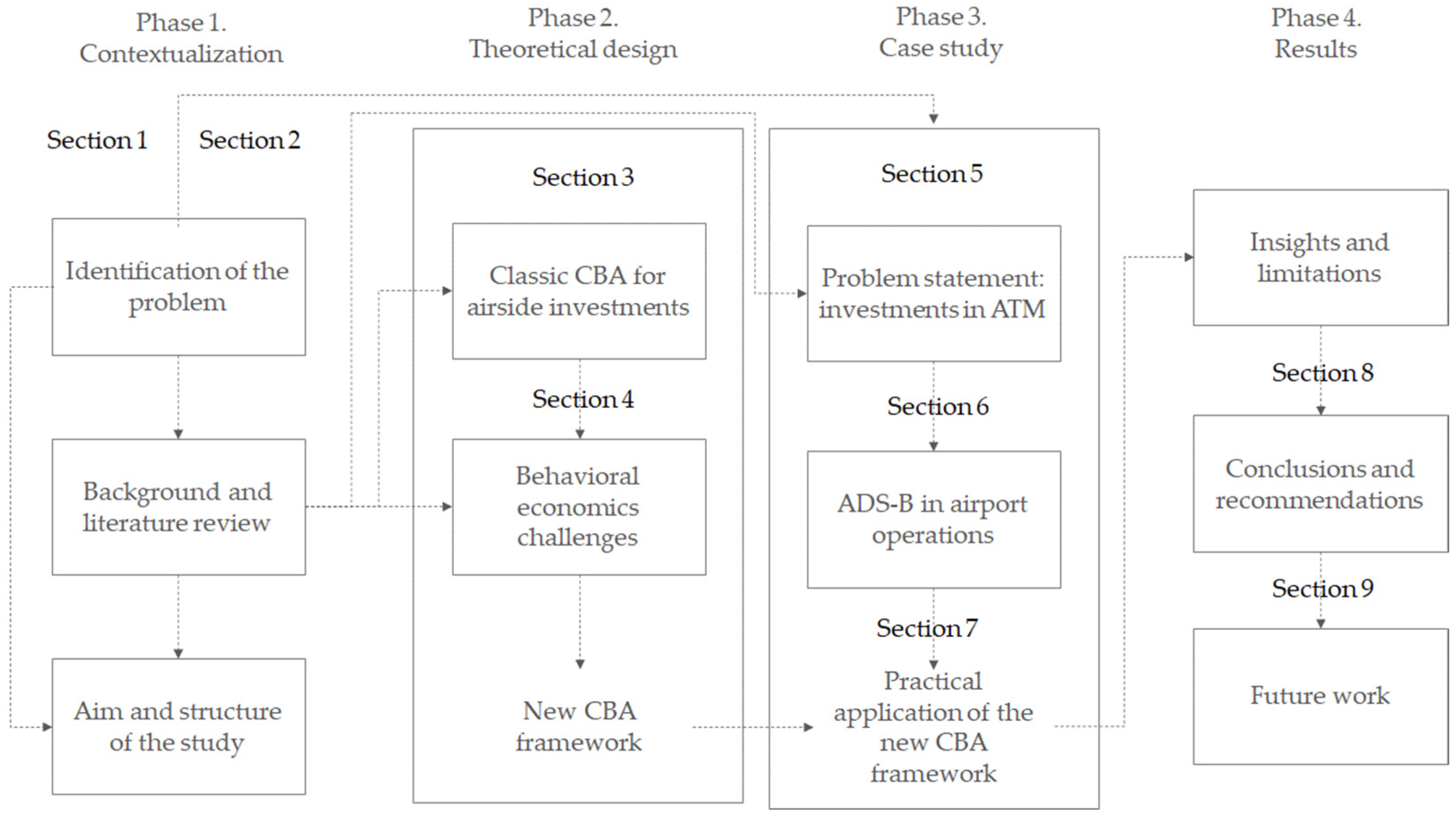
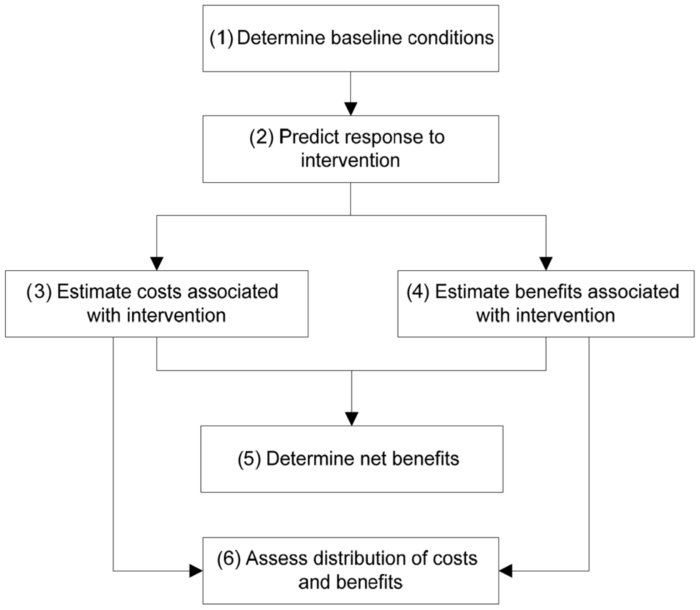
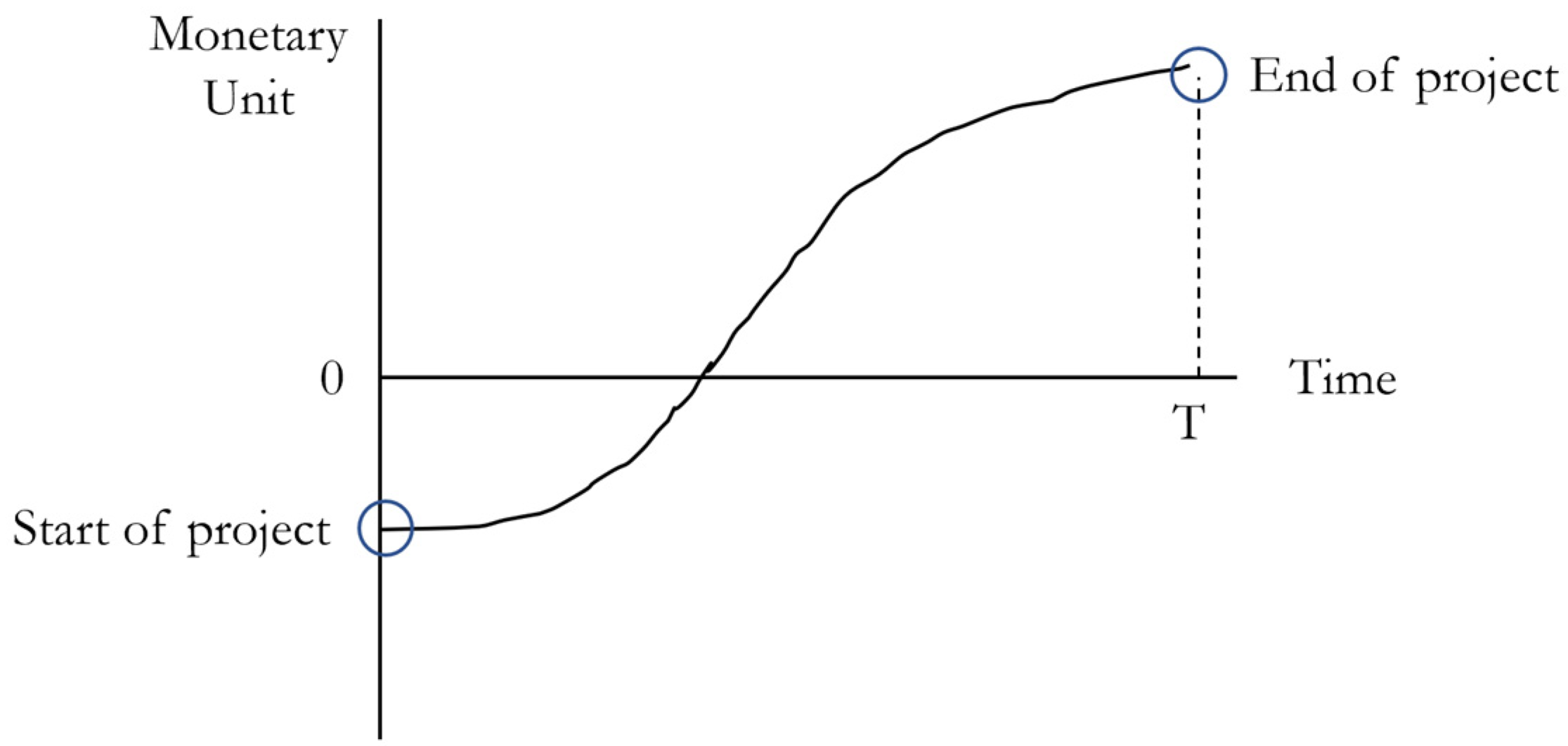
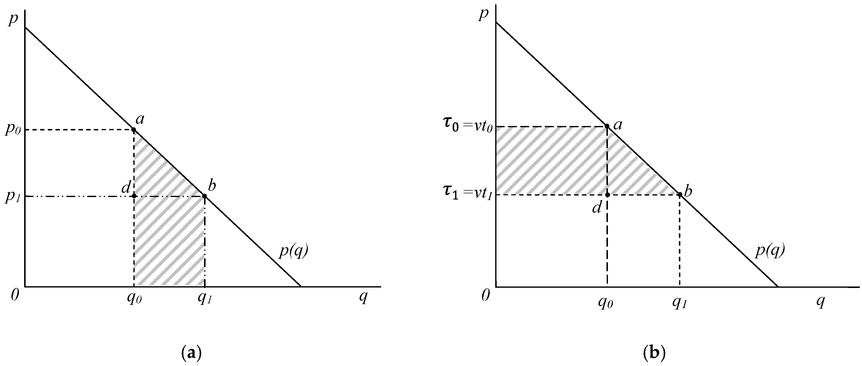
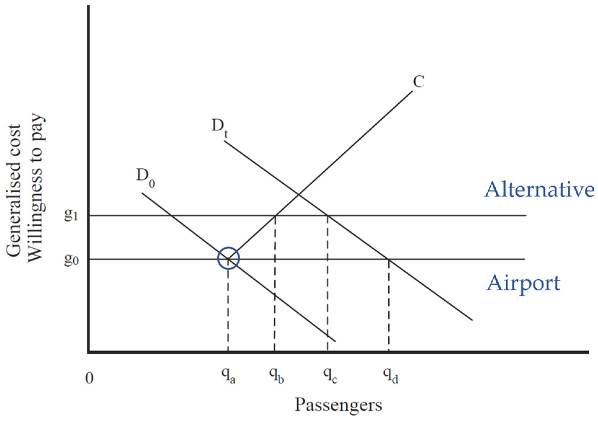
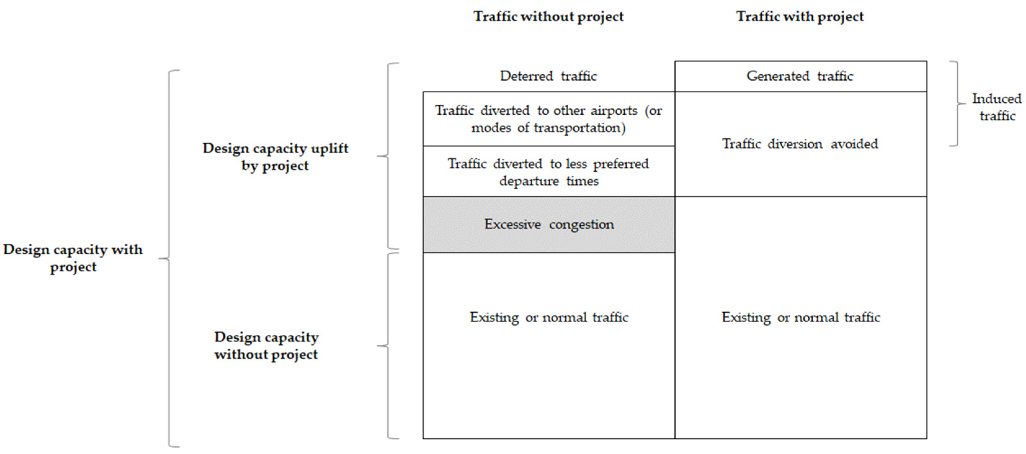
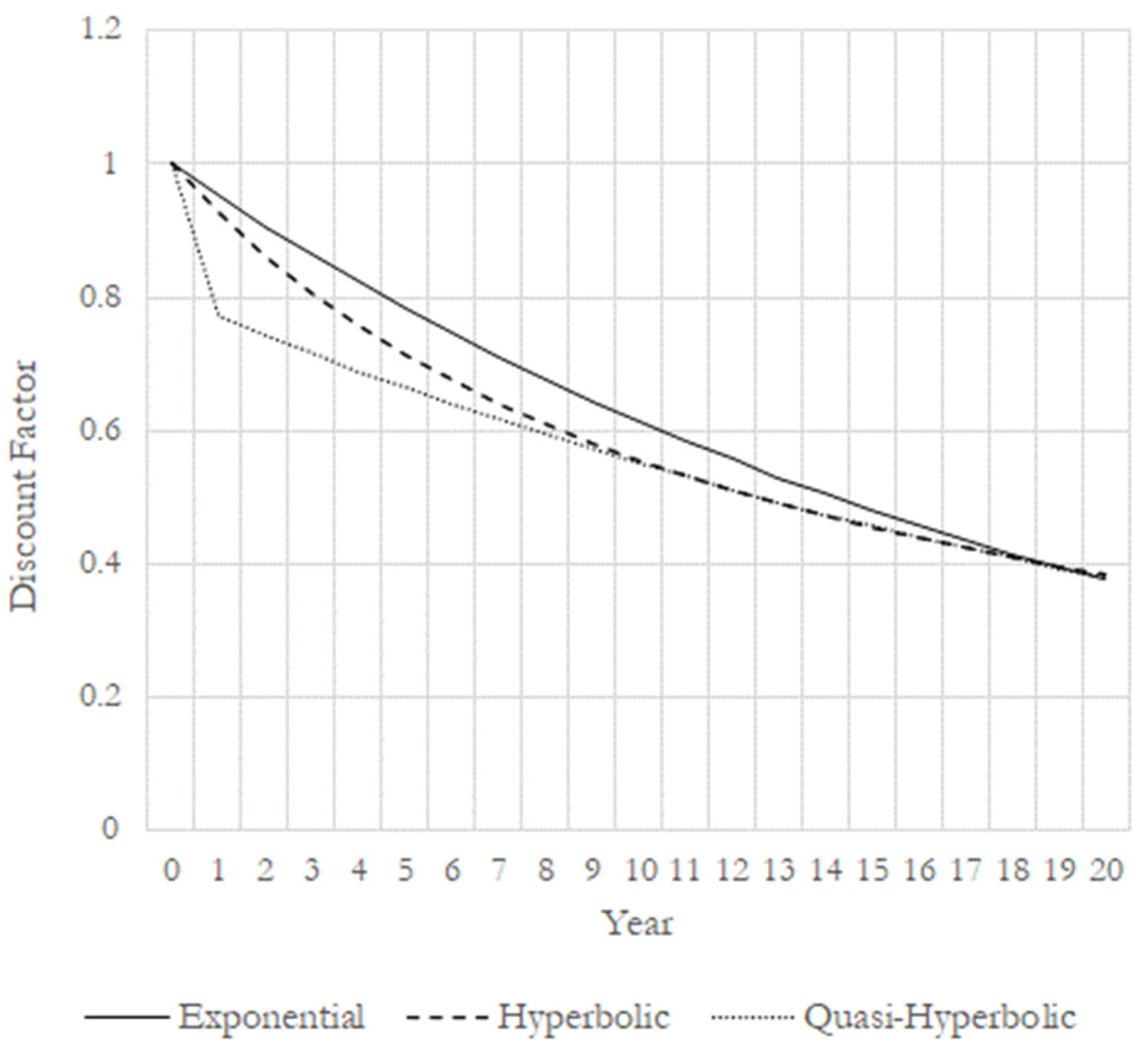
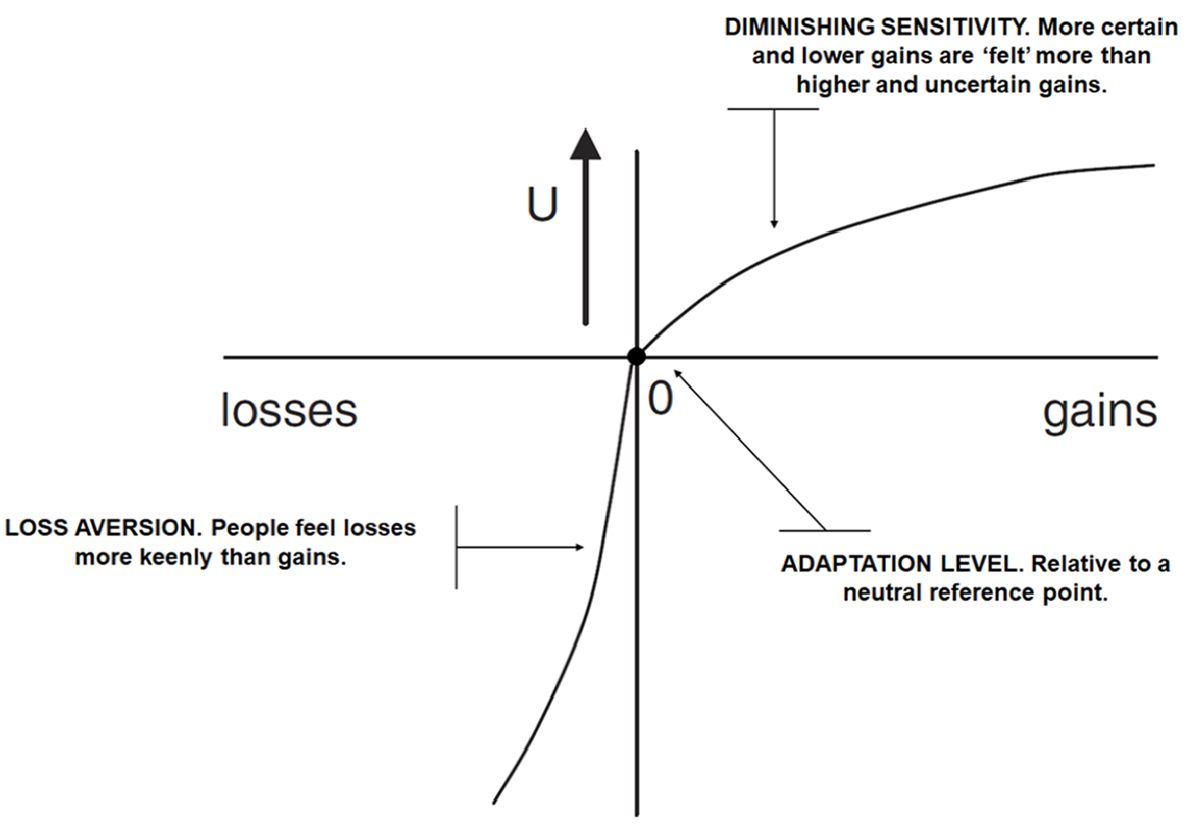
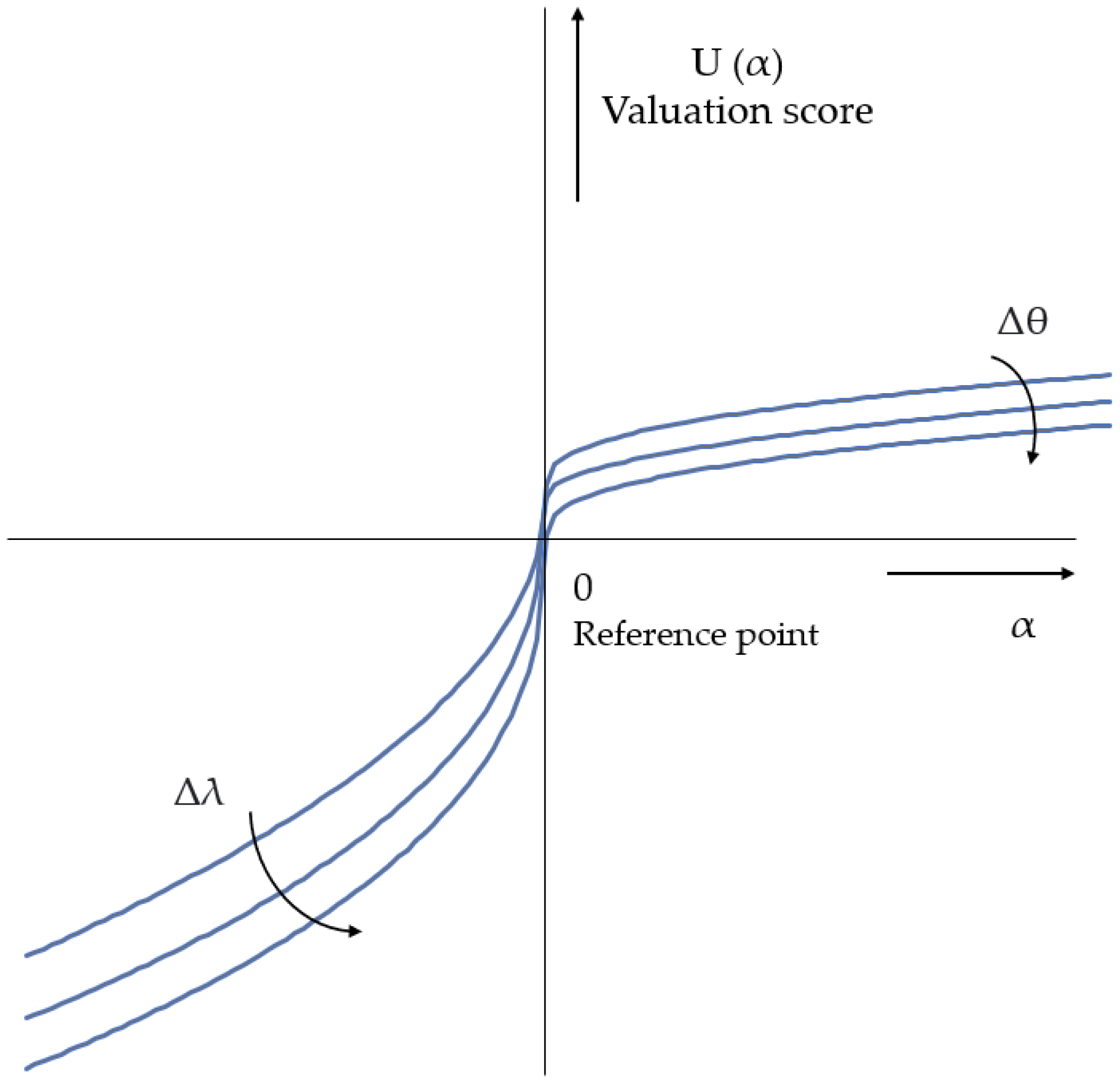
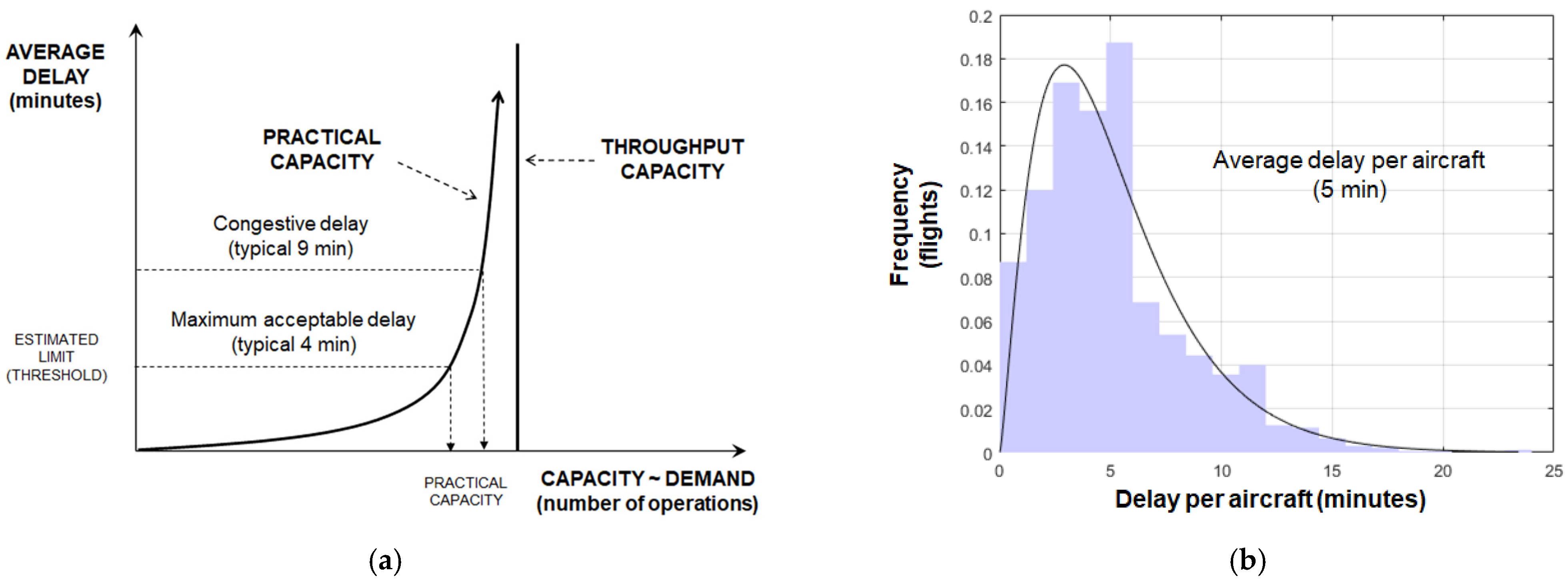
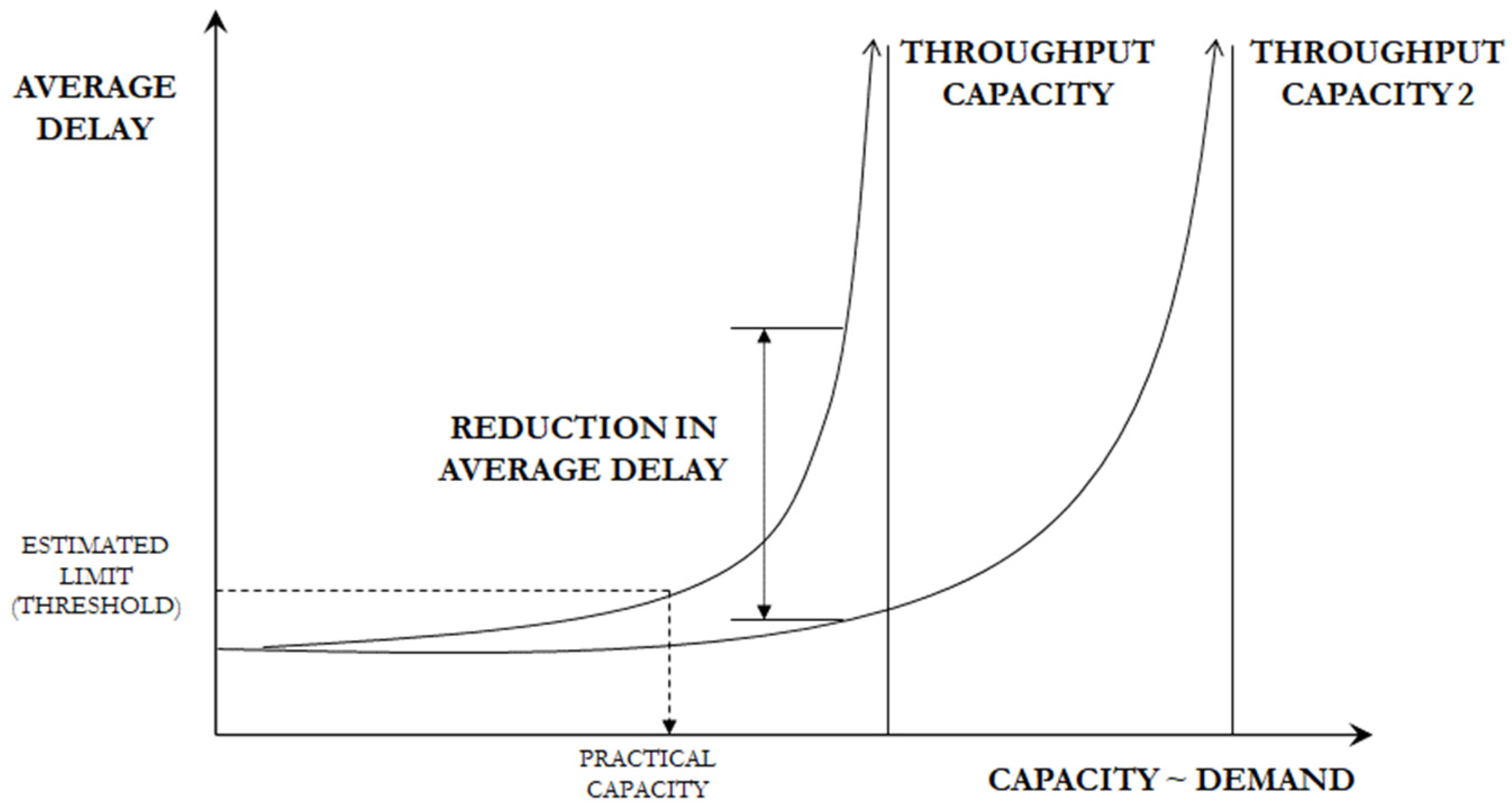
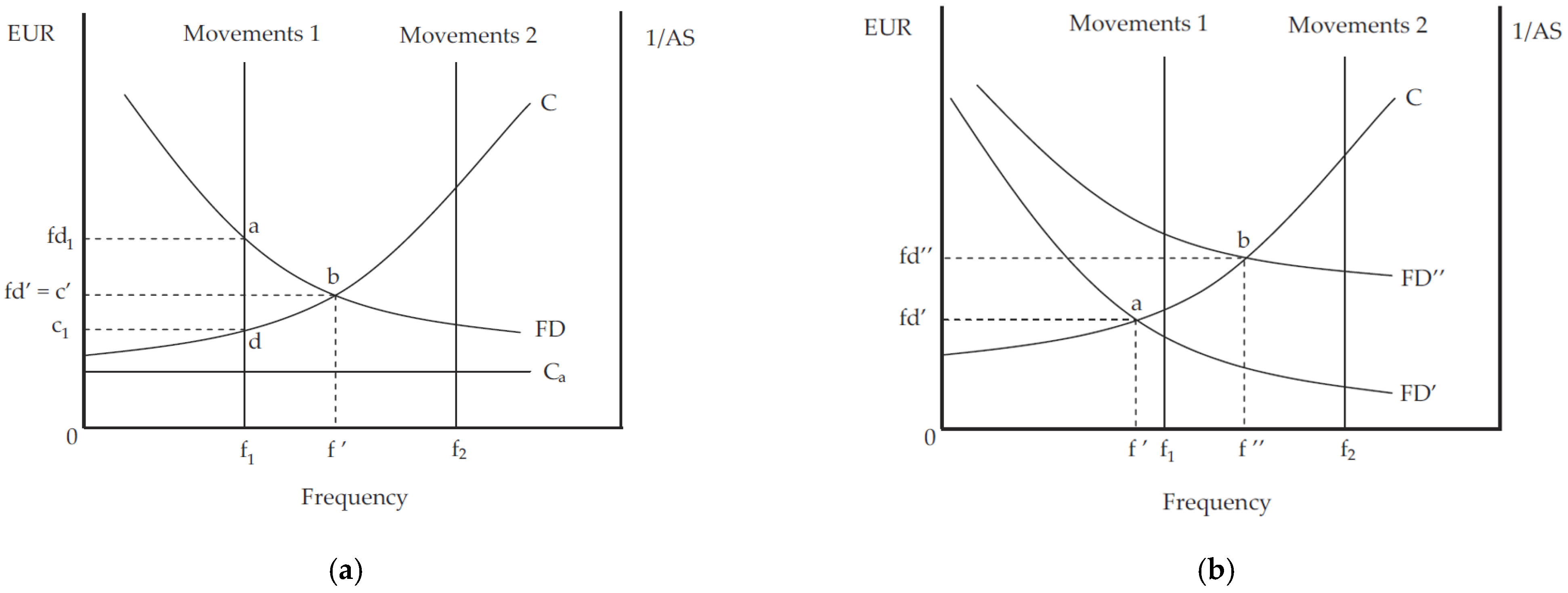
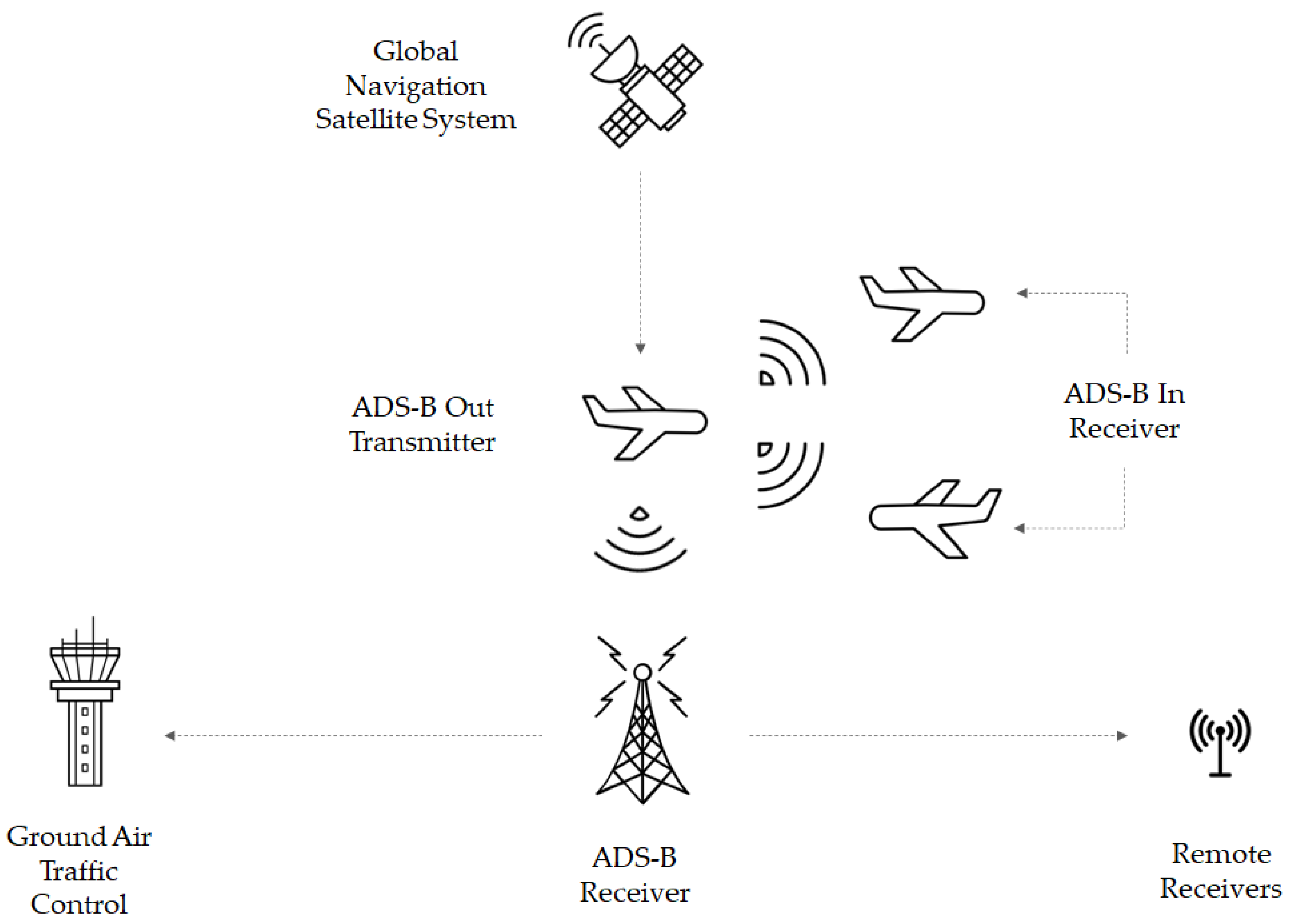
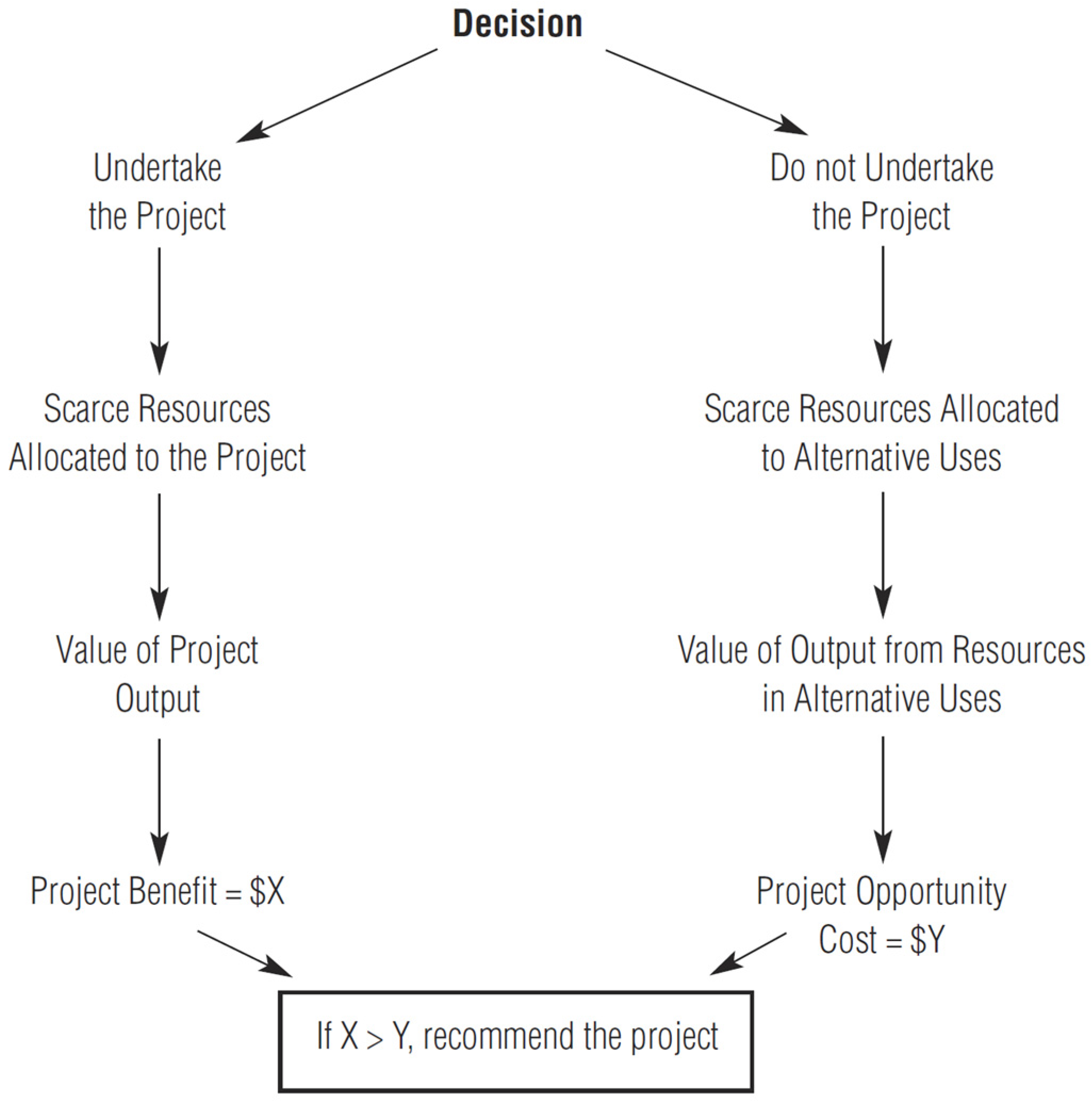
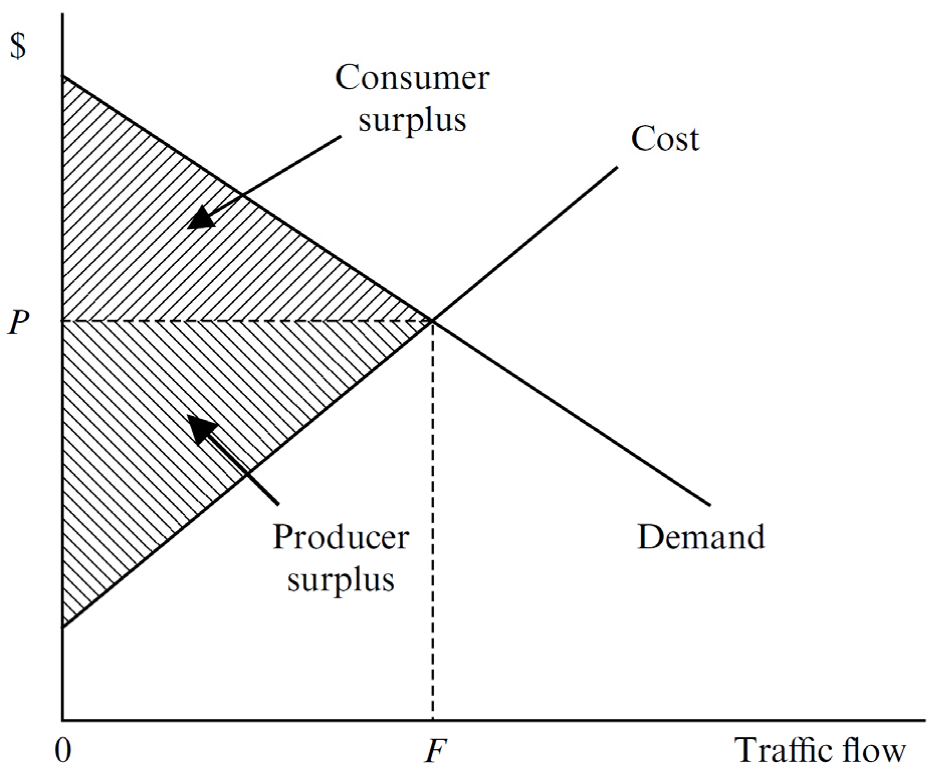
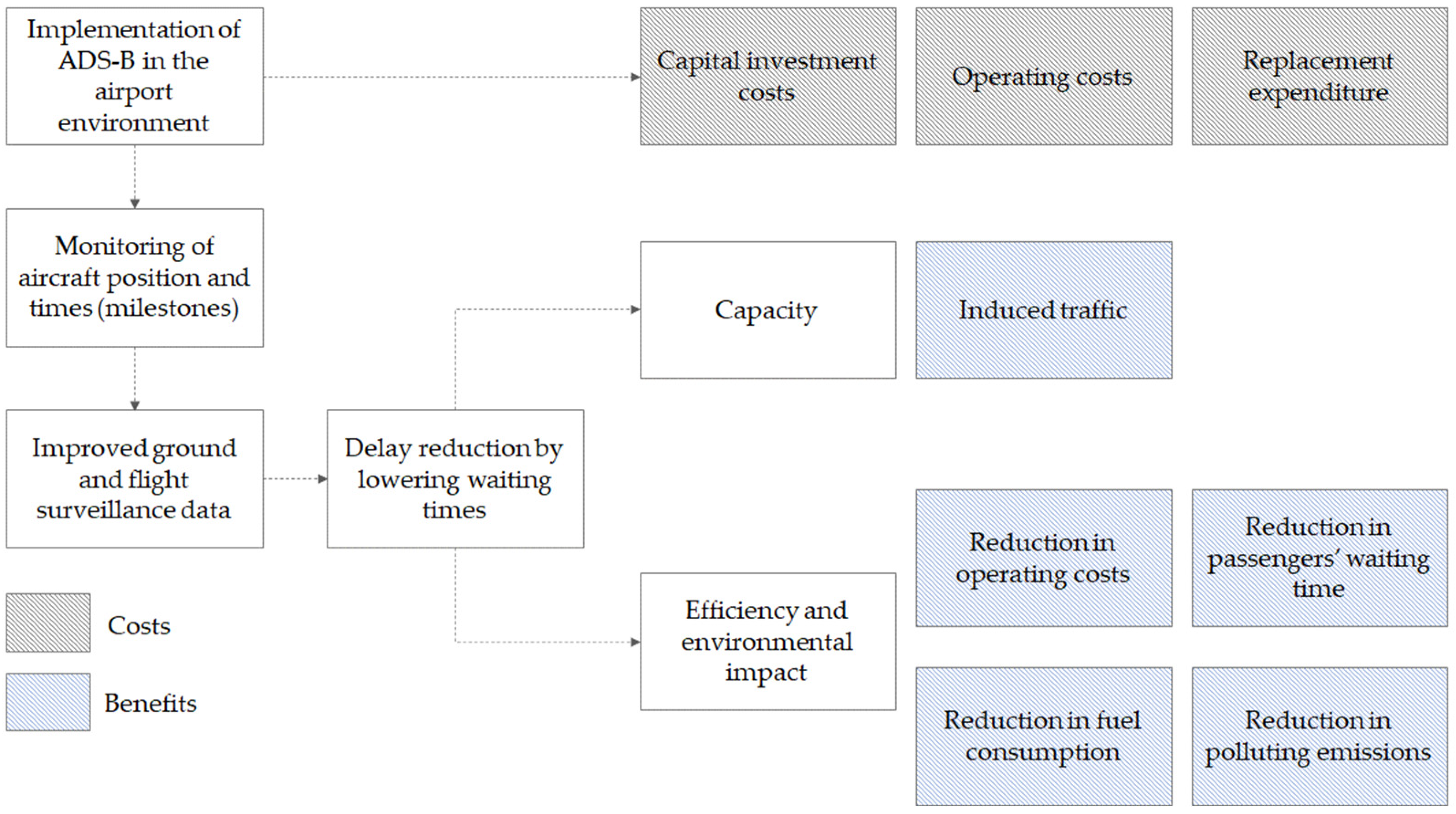
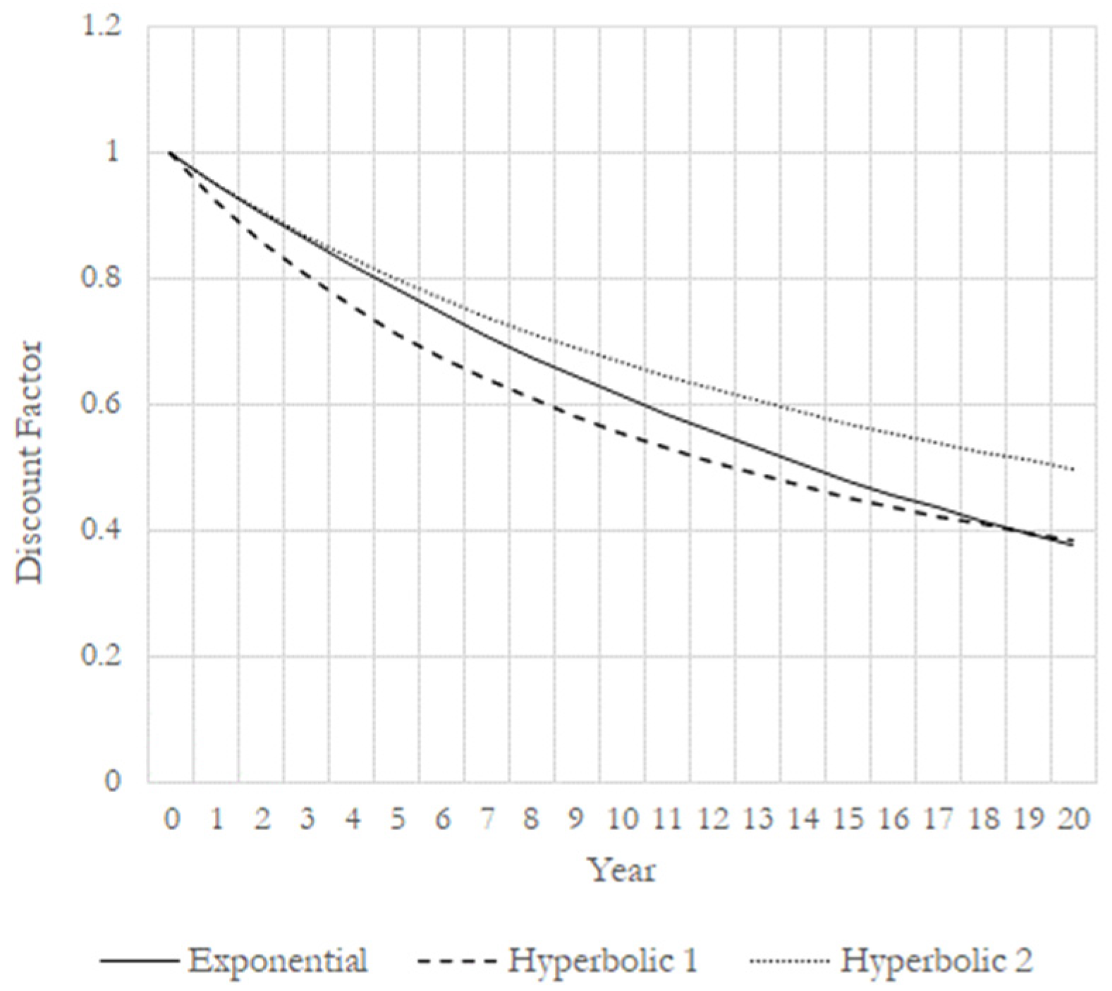
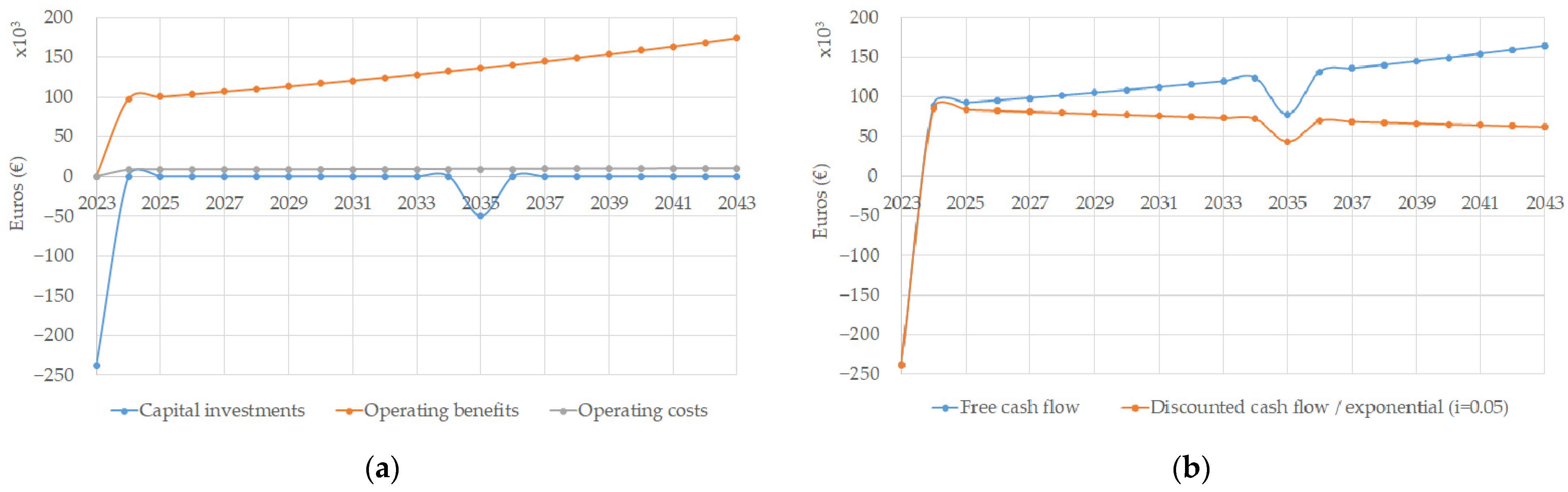
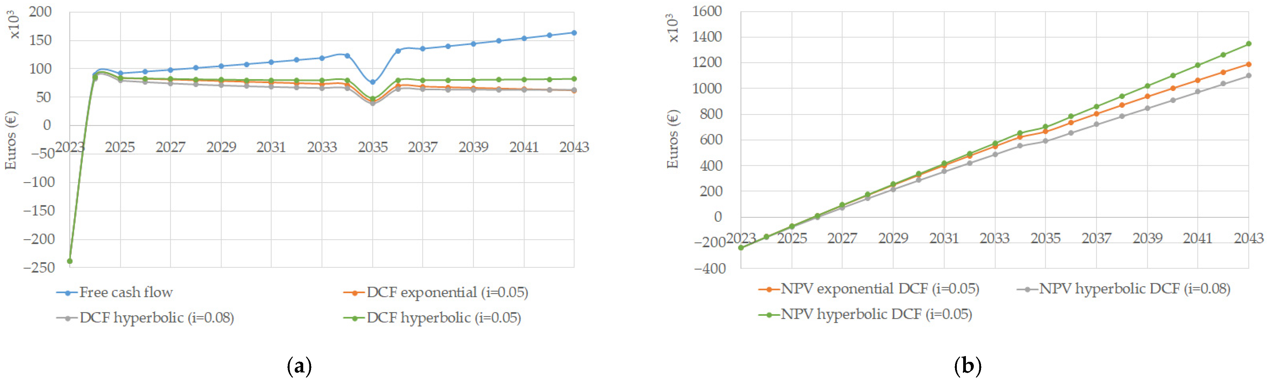
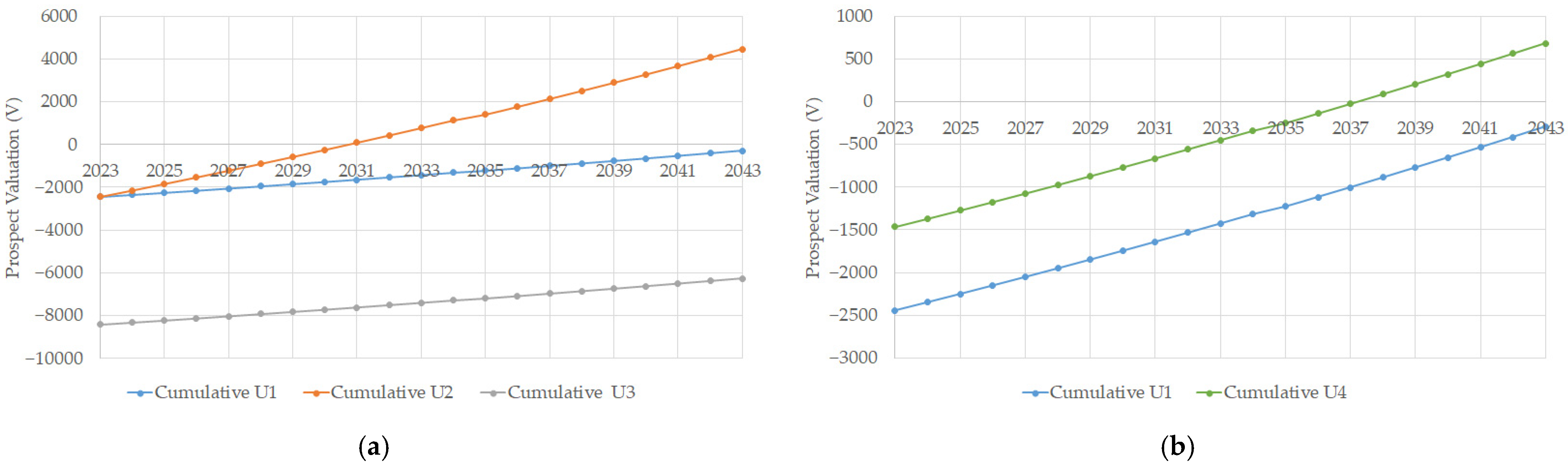
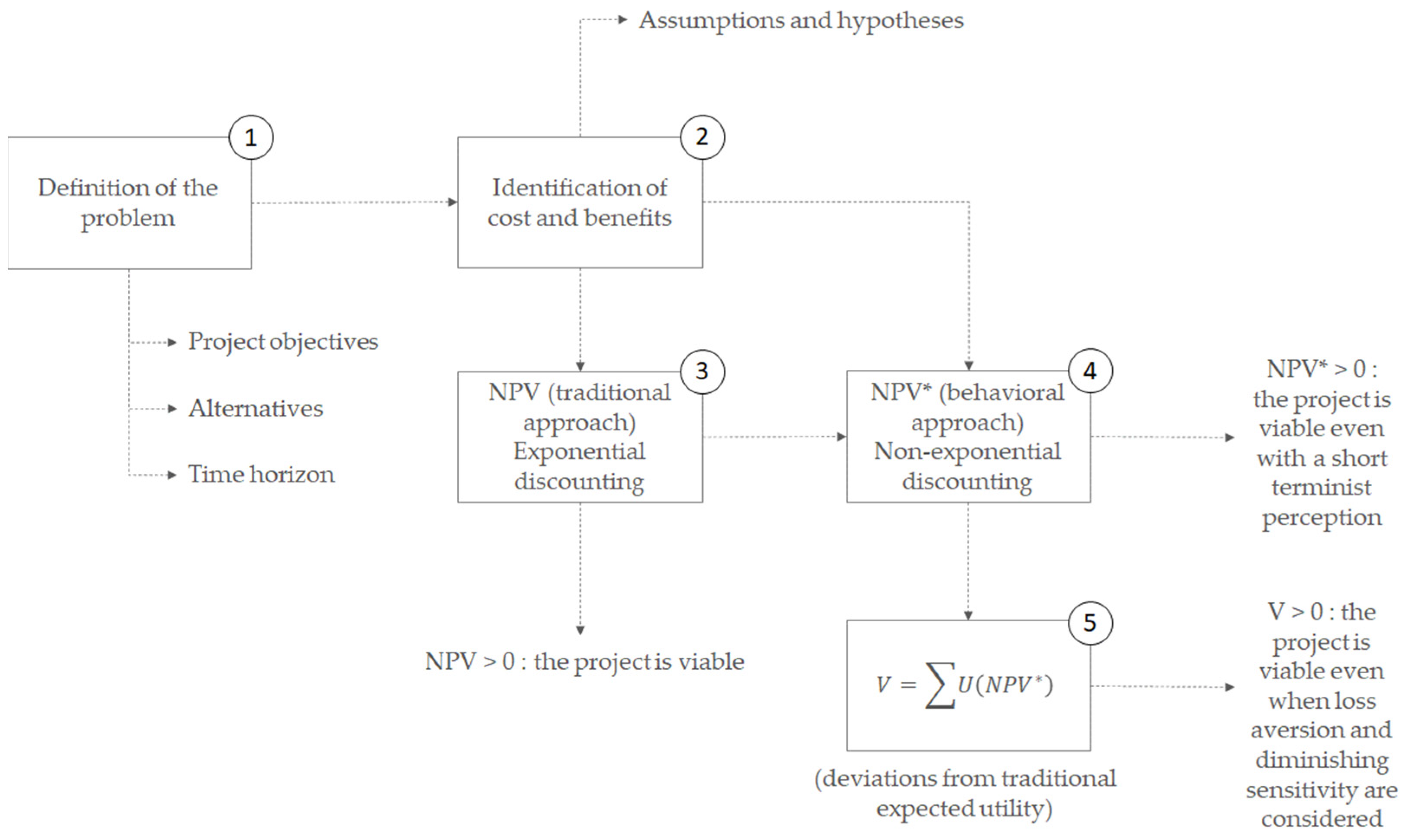