
A New Adaptive Control Algorithm of IGC System for Targets with Several Maneuvering Modes Based on GTSMC-DNN

1
School of Astronautics, Beijing Institute of Technology, Beijing 100081, China
2
Shanghai Institute of Mechanical and Electrical Engineering, Shanghai 201109, China
*
Author to whom correspondence should be addressed.
Aerospace 2023, 10(4), 380; https://doi.org/10.3390/aerospace10040380
Submission received: 1 February 2023
/
Revised: 31 March 2023
/
Accepted: 17 April 2023
/
Published: 19 April 2023
Abstract
:To improve the performance of intercepting a target with different maneuvering modes and changing the mode suddenly during the interception, a new adaptive control algorithm for the IGC (Integrated Guidance and Control) system is proposed, using the global terminal sliding mode control method and a DNN (Deep Neural Network). Firstly, the missile-target problem is formulated and a new strict-feedback nonlinear IGC model with mismatched uncertainties is established. Secondly, the paper divides the IGC system into four subsystems, including a guidance subsystem, overload subsystem, attitude subsystem and the deep neural network subsystem. To transform the control signal between each subsystem and avoid the “differential explosion” problem, the paper defines the SOF (Second Order Filter). Thirdly, in combination with a deep neural network, a new modified global terminal sliding mode surface and the adaptive control law are designed. At last, using the Lyapunov theory, the stability of the IGC system is analyzed. Finally, to illustrate the effectiveness of the proposed algorithm, several simulation cases are given. The simulation results show the superiority of the proposed algorithm in adapting different maneuvering modes during the whole interception, improving the control performance and having a high interception accuracy.
1. Introduction
Nowadays, with the development of aviation and aerospace technologies and the better performance of missile guidance and control (G&C) systems, precise strikes have become easier to achieve in modern military affairs, especially in the Gulf war (1991), Afghan war (2001), Russia–Ukraine war (2022) [1], etc. As is known to all, when designing a new guidance and control system for a missile, the traditional process often splits the missile into a guidance loop (guidance law) and a control loop (autopilot). The traditional method can intercept a target with little or no maneuvering capability. In terms of intercepting high speed and great maneuvering targets, the coupling effect between the control subsystem and the guide subsystem must become stronger. Moreover, the performance of the missile may degrade, and the closed loop of the missile may even become unstable. Thus, the IGC system has lately attracted the attention of researchers, due to much consideration about the coupling between the control subsystem and the guide subsystem. Compared with the traditional design process, the IGC system can fully consider the coupling effect between the guidance system and the control system. Thus, the IGC system is better suited to intercept maneuvering targets. Furthermore, using the IGC system can also reduce the iterative process, which may speed up the rate of progression of a new missile. Therefore, many studies have investigated the IGC controller design. In terms of interception with an impact angle constraint, a novel integrated guidance and control (IGC) law, which uses the high-order fully actuated system approach and the cascaded linear extended state observer (LESO), was researched in [2]. To solve the problem of a maneuvering target, a new sliding mode control algorithm was proposed in [3]. For this approach, the researchers used the liner sliding mode surface, which may have been unable to determine the convergence time. The state-of-the-art integrated guidance and control (IGC) systems were discussed in [4]. Furthermore, the study envisages that artificial intelligence (AI) will become the future research direction, especially in the research of intelligent neuro-fuzzy systems. However, this paper did not describe how to implement the AI approaches specifically. To address the problem of intercepting a maneuvering target with a desired terminal impact angle, a new guidance law based on a nonlinear relative virtual guidance model and the optimal control was proposed in [5]. To solve the problem of partial measurement information and unmatched uncertainties in strap-down hypersonic flight vehicles, a new IGC control scheme was proposed in [6] by combining with the barrier Lyapunov function, backstepping methodology and the finite-time disturbance observer. Although this method has several highlights, it does not take the dynamics of the actuator into account. By using the observer to estimate the target maneuver and disturbance information for the guidance law design, a new IGC law with impact-angle constraints utilizing DSC and N-ESO was proposed in [7]. Although this method has several highlights, it does not take the actuator saturation into account. In [8], the RG (reference and command governors) approach was proposed, which assumes that the inner loop can track the reference trajectory, with fine disturbance rejection capability in the cases without constraints. A certain constrained optimization algorithm was then exploited to generate the reference trajectory so as to prevent constraint conflicts with the receding horizon strategy. However, the high calculation cost makes them implementable only with a low sampling rate. In [9], considering the impact time constraint, a new fixed-time nonlinear circular guidance law was designed for intercepting a stationary target. However, this method may not be suitable for intercepting a maneuvering target. In [10], a novel non-singular terminal sliding mode control-based integrated missile guidance and control system with impact angle constraint was proposed. While this approach divided the IGC system into a guidance system and a control system, each subsystem was designed separately. Considering the input saturation and constraints of the attack angle, sideslip angle and velocity deflection angle in the IGC system, a novel adaptive IGC scheme was proposed by combing dynamic surface control with a barrier Lyapunov function (BLF) in [11]. However, the interception performance was not better when the target had a larger maneuver. Considering the intercept impact angle, an analytical solution for the interception of a fixed target was proposed in [12] by using the pure PNG law. Using this approach, the researchers established the relationships between the intercept impact angle, the initial relative motion state and the PNG coefficient. Based on this, they derived an analytical expression for the intercept impact angle. In [13], the researchers designed an impact-angle-constrained suboptimal guidance law using the state-dependent Riccati equation (SDRE) technique and addressed the terminal acceleration constraint by adjusting the guidance coefficients. However, these guidance laws often assume that the target is stationary and, thus, do not perform well when the target is maneuvering. In [14] the researchers proposed a three-dimensional guidance law for intercepting a maneuvering target with both impact angle and impact time constraints in which the quadratic LOS profiles in the pitch and yaw planes were suggested, respectively. Assuming that the LOS angle could be shaped as a polynomial function of range-to-go, an impact time constrained guidance law using a range-based line-of-sight shaping strategy was proposed in [15]. Treating the heading angle, LOS angle and flight time as state variables, a new linearized dynamic model of the missile was proposed in [16]. Based on this, a highly constrained guidance algorithm was investigated, and a generalized semi-analytical solution for a guidance command with IAT constraints was derived. In [17,18,19], the SMC methods were also employed to control the impact time. Many impact time control guidance laws based on SMC methods have complicated structures, making it stressful to deal with the look angle constraint. Moreover, to satisfy impact time constraint, guidance gains or parameters are often tuned by trial and error, or by using an optimization routine, which can make online calculations less efficient. In [20], a novel fixed-time distributed cooperative guidance law with impact angle constraint is proposed to solve the guidance problem of multiple missiles attacking a maneuvering target simultaneously in plane. By using the nonsingular terminal sliding mode control, it designs a cooperative guidance law on the line-of-sight (LOS) direction, which can guarantee that all missiles hit the maneuvering target simultaneously. Combining repetitive control (RC) with a sliding mode control method, a three-dimensional homing guidance law with impact angle constraint is proposed in [21]. However, this approach did not consider the dynamics of the rudder. Considering the impact time and the impact angle constraints, a new shaping approach in proposed to increase the mission effectiveness in [22]. In addition, to the shaping of the look angle, the guidance law in [23] is derived by shaping the range as a time-dependent polynomial. The method also solves the impact time problem under the look angle constraint, showing robustness under lagged response and seeker noise. In terms of the excessive acceleration change in the terminal control stage by PNG, a new strategy for acceleration threshold control based on the gravity-compensated PNG law is proposed in [24]. To attack a stationary target with the desired impact angle and time, a new nonlinear guidance law is developed in [25]. Using this method can solve the problem indeed. However, this method is more suitable for intercepting a stationary target. Additionally, to hit the stationary ground targets in the specified direction, a nonlinear impact angle control guidance law based on Lyapunov stability theory is proposed in [26]. However, this method just considers how to intercept stationary ground targets. For maneuvering targets, this approach has not been investigated. Based on the analysis of the classical state-dependent Riccati equation scheme, a new three-dimensional guidance law was designed in [27]. However, this research did not take any constraints into consideration. To solve the finite-horizon tracking problem for input-affine nonlinear systems with specified terminal conditions, an impact angle guidance based on finite-horizon robust optimal control is proposed in [28]. In [29], using reinforcement learning, a new guidance law that uses observations, consisting solely of seeker line-of-sight angle measurements and their rate of change, is presented. However, the simulation result is not better when intercepting great maneuvering targets. In terms of the aerodynamic uncertainty and strong nonlinearity in the high angle-of-attack (AOA) flight phase, an all-aspect attack guidance law is proposed in [30]. However, this method has a fatal disadvantage; the method must have sufficient training data obtained from CFD (Computational Fluid Dynamics). In addition, the real-time performance is unsatisfactory. Considering the time and field-of-view (FOV) constraints, a new homing missile guidance law, which uses the sliding mode control method, is presented in [31]. Relying on model linearization, a FOV limited-time and angle constraint optimal guidance law was proposed in [32]. However, it is forced on the stationary target. To guarantee that the LOS angle tracking errors are zero, a new fast fixed-time nonsingular sliding manifold was designed in [33]. In this approach, when designing the novel sliding mode reaching law, the sat function is used to weaken the chattering phenomenon. However, this method was only suitable for targets with little or no maneuvering capabilities. In [34], considering the impact angle constraint, a new cooperative guidance law for attacking the ground target was presented. In [35], to improve the accuracy of interception, a novel continuous adaptive finite time guidance (CAFTG) law was presented for homing missiles. In this approach, the nonlinear disturbance observer and sliding mode control theory are used to estimate the acceleration of a target and guarantee finite time convergence. In [36], considering the impact time constraint, an ITCG strategy was presented based on the exact time-to-go solution. In this method, the important parameters in terms of the initial configuration can be found based on the impact time analysis. In [37], a three-dimensional (3D) robust guidance law was proposed for bank-to-turn (BTT) missiles against the couplings and target maneuver. In this approach, to indicate whether they strengthened or weakened the system stability, a new QI (Qualitative Indicator) was designed based on the Lyapunov stability theory for both coupling and target maneuvering terms. To fight against maneuvering targets with terminal angle constraints, a new three-dimensional guidance law based on the time-varying sliding mode control methodology was proposed in [38]. This approach used the fractional power-extended state observer to estimate the unknown target acceleration and reduce the adaptive switching gain. Then, a newly sliding mode surface was established by introducing a time base generator function. Considering different seekers’ field-of-view (FOV) constraints, a new distributed three-dimensional (3D) nonsingular cooperative guidance law was proposed for multiple missiles in [39]. However, this method may not be suitable for intercepting maneuvering targets, especially intercepting a target with different maneuvering modes. To analyze the capture region of the composite guidance law for a missile with a strapdown seeker, a FOV and angle constraint guidance law was derived in [40]. Considering the time-varying speed, a new look angle shaping guidance law with an impact angle and seeker’s field-of-view (FOV) constraints was proposed in [41]. However, the derived law can only intercept stationary targets. Considering the lateral acceleration limit, the field of view limit and the sensor measurement noises, a new three-dimensional guidance law with a multi-constrained interceptor was proposed in [42]. In this method, the extended Kalman filter was used to estimate parameter uncertainties and to filter out the noises.
In summary, all above approaches have been researched to solve the IGC problem. However, when the target has different maneuvering modes and changes the maneuvering mode suddenly, the interception performance will become worse. Therefore, to solve this main problem, the paper proposes a new adaptive control algorithm for IGC system by introducing a deep neural network to the system. In this paper, the IGC system is divided into four subsystems, including the guidance subsystem, the overload subsystem, the attitude subsystem and the deep neural network subsystem. Considering the uncertain items and the adaptive item, a new fourth order IGC model is established. In this model, to transform the control signal between each subsystem and avoid a “differential explosion”, a new second order filter is defined. Finally, using the terminal sliding mode control method, the second order filter and the deep neural network, the paper designs the adaptive controller for IGC system. The main advantage of the method is that it cannot only increase the convergence speed of the system states, but can also improve the adaptive interception capability of the missile. Thus, the main contributions of this study are as follows:
- 1.
- In order to improve the adaptive interception capability of the missile, a new adaptive IGC nonlinear mathematic dynamic model with deep neural network is established. In this model, the IGC system is divided into four subsystems including guidance subsystem, overload subsystem, attitude subsystem and the deep neural subsystem.
- 2.
- Aiming to transform the control signal between each subsystem and avoid the “differential explosion”, the paper defines a new SOF (Second Order Filter). Additionally, to formulate the uncertain items, the paper defines the corresponding equation.
- 3.
- Combined with GTSMC, SOF and DNN, the paper designs a new IGC adaptive controller to intercept the maneuvering target, which has different maneuvering modes and changes the maneuvering mode suddenly during the interception process.
- 4.
- Using Lyapunov’s theory, the closed-loop system was proved to be stable. Finally, several simulation results demonstrated the superiority of the method proposed in this paper, compared with the previous approaches.
In short, the paper is organized as follows: the introduction is stated in Section 1. Then, the target with different maneuvering mode, the missile-target interception problem and the dynamics model of the missile and IGC dynamic model with uncertain items are formulated in Section 2. The adaptive controller is designed by combining deep neural network and the global terminal sliding mode control in Section 3. The stability of the closed-loop system is proved using Lyapunov’s theory in Section 4. The simulation results and analysis are presented in Section 5. Finally, the conclusions are summarized in Section 6.
2. Problem Formulation
In this section, the engagement kinematics of missile-target will be formulated. Then, the paper will drive the strict-feedback IGC model with deep neural network in the pitch plane.
Before establishing the engagement kinematics, the paper will introduce the interception scenario where the target has different maneuver modes. The interception scenario is shown in Figure 1.
As shown in Figure 1, it is clear that the target maneuver modes consist of two phrases during interception. In the first phrase, the target adopts the S-type maneuver mode to avoid the missile. As the missile approaches the target, the target makes a vertical maneuver suddenly to avoid being intercepted. It is obvious, according to the real-time battlefield, that the target can adopt various maneuver modes to avoid being intercepted. Thus, this will become a great test for the interceptor, because the current interceptor’s control and guidance parameters are fixed. In these conditions, the interceptor’s performance is comparatively poor, when facing the rapidly changing battlefield. Thus, to improve the adaptive capability of the missile, the paper introduces the deep neural network to the control system and derives the corresponding adaptive guidance law.
2.1. Engagement Kinematics
Before establishing the dynamics of the missile-target and the strict-feedback IGC model with deep neural network, the following assumptions will be considered for analyzing and designing of the control law.
Assumption 1.
The speed of a pursuer is constant.
According to the real battlefield shown in Figure 1, we can obtain the relative motion of the missile–target, and its pursuit is shown in Figure 2. At the same time, the dynamics of the missile steered by the tail aerodynamic control surfaces in the pitch plane is shown in Figure 3.
As can be seen in Figure 2, which gives the pursuit geometry of the missile–target in the pitch plane, denotes the relative distance between the missile and the target. denotes the inertial coordinate system. , and denotes the velocity, the flight path angle, and the acceleration of the target, respectively. Similarly, , and represent the velocity, the flight path angle, and the acceleration of the missile, respectively. is the LOS angle. and denote the position of the missile and target. is the missile body axis, and is the pitch angle of the missile.
As can be seen in Figure 3, which gives a schematic of the missile in the pitch plane. denotes gravity. and denote the aerodynamic drag and the lift force of the missile, respectively. In addition, represents the attack angle.
According to all the conditions above, when assuming , the dynamic equations of the missile-target can be written as follows:
Differentiating Equation (2) with respect to , which can be obtained as:
where and are defined as .
2.2. The Missile Dynamics with Uncertain Items
In this subsection, the paper will derive the dynamic equation of the pitch plane and define the corresponding uncertainties in the IGC model. The planar dynamics is formulated as follows:
where denotes the attack angle. represents the mass. is the pitch angular rate. denotes gravitational acceleration. is the moment of inertia. denotes the pitch angle. and are the aerodynamic lift force and pitch moment, respectively. and can be written as follows:
where . and are the reference area and the reference length, respectively. is the rudder deflection angle. In addition, denotes the lift force derivative with respect to . and denote the pitch moment.
According to Equations (1) and (4), then the missile normal overload can be derived as follows:
then, the normal overload can be written as follows:
where is determined by aerodynamic parameters.
When designing a new missile, people often use wind tunnel experiments to obtain the force coefficients and moment coefficients. However, these values are usually inaccurate. Thus, considering these uncertainties, all these coefficients can be written as follows:
where and represent the uncertain terms which are continuous and satisfy the following condition:
According to Equations (1)–(9), the missile dynamic model with uncertain items can be written as follows:
where are defined as follows.
2.3. Fourth-Order IGC Model in State Space
Before establishing the IGC model with a strict-feedback state equation, the system parameters can be defined as follows.
To solve the problem of satisfying the impact angle constraint, we can define the desired terminal LOS angle , which satisfies . Then, the paper defines the flowing state vector:
According to Equations (2) and (3) and Equations (10)–(12), the IGC dynamic model in state space can be written as follows:
where the control input . , and are defined as follows:
Now, the paper obtains the IGC dynamic model with uncertain items.
3. Adaptive Controller Design with Deep Neural Network
In this section, the paper will design an adaptive controller by using the DNN (deep neural network) and the GTSMC algorithm for the uncertain dynamic model formulated in Equation (14).
3.1. Design Objectives
In this paper, the new adaptive IGC law satisfies the following conditions. Additionally, the structure of the proposed approach is shown in Figure 4.
The objective of this paper is as follows:
- (1)
- The LOS angle can be soon converged to the desire angle ;
- (2)
- The controller has a strong adaptability against maneuvering targets with different maneuver modes;
- (3)
- When considering the relationship between each control loop, a small miss distance can be achieved;
- (4)
- The stability of the closed-loop system of the system states should be ensured.
3.2. Deep Neural Network
To improve the adaptability of the missile, a DNN (deep neural network) is introduced to the system. The typical structure of DNN is shown in Figure 5.
Like other neural networks, the deep neural network also consists of an input layer, a hidden layer, and an output layer. In hidden layers, each neuron is fully connected, meaning any neuron in hidden layers must be connected with any neuron in hidden layers and . According to the specific problem, we can construct the appreciate networks with different hidden layers. As shown in Figure 5a, denotes the input vector, and is the th element of . represents the weight from the th neuron in the th hidden layer to the th neuron in the th layer. denotes the output vector, as can be seen in Figure 5b, which gives the computational structure of neurons. denotes the th neuron in the th layer. denotes the th bias in the th layer. is the neuron output. denotes the activation function, whose input is . To improve the convergence speed, is defined as follows:
To design the adaptive control law, the paper defines that is the optimal value of the deep neural network. Then, we will obtain the following equation.
Thus, choosing different hidden layers, we will obtain a different deep neural network adaptive value .
3.3. Second Order Filter Definition
In this paper, the IGC system will be divided into four subsystems: the guidance subsystem, the normal overload subsystem, the attitude subsystem and the neural network subsystem. To avoid the “differential explosion” phenomenon caused by the Backstepping control method, the paper defines a new second-order filter as follows:
In Equation (18), are the filter parameters, which are all constant.
Then, the filter error is defined as follows:
Differentiating and combining with Equation (17), can be obtained as follows:
The system states are continuous and bounded. Thus, those will have the positive constants , which satisfy the following condition:
3.4. Adaptive Control Law Design Based on GTSMC-DNN
As we know, the conventional SMC method often chooses a linear sliding mode surface which has a fatal disadvantage: the tracking errors cannot converge to zero in a finite time. In addition, the adaptive ability of this approach is very poor. Therefore, in this paper, we hope that the tracking error of LOS can converge to zero within a designated time and the controller can have a better adaptive ability, when intercepting the target with various maneuvering modes. Thus, a new modified global terminal sliding mode surface will be designed, combined with the deep neural network.
Remark 1.
In this paper, the purpose of missile control is that the LOS angle is equal to desire angle and .
- Step 1: guidance subsystem with DNN
In this subsystem, this paper will use a two layer deep neural network. The input layer includes five neurons. The output layer has a signal neuron, which will output the adaptive normal overload command . The structure is shown in Figure 6.
As can be seen in Figure 6, the input vector is defined as and the weight vector is defined as . Thus, the output of the neural network can be written as follows.
According to Equation (14), are related to the . To ensure the desired LOS angle and realize . The new sliding mode surface is designed as follows:
where are the state variable. and are positive constants. and are positive odd integers which satisfy .
Then, the corresponding reaching law is defined as follows:
where and are all positive odd constants. determines the reaching speed. denotes the optimal weight coefficient matrix. denotes the optimal bias.
According to the control structure in Figure 4, when introducing the DNN into guidance subsystem, can be written as . Combining Equations (14), (15), (17) and (24) and differentiating Equation (23), we can design the virtual command of the guidance subsystem with the deep neural network:
As is continuous and has not switched items, according to SOF, is made to passes through the SOF to obtain .
- Step 2: overload subsystem with DNN
In this subsystem, the paper will use a two layer deep neural network with a signal input layer and a signal output layer. The input layer includes four neurons. The output layer also has a signal neuron, which will output the adaptive pitch angular rate command . The structure is shown in Figure 7.
As can be seen in Figure 7, the input vector is defined as and the . Then, the output of the neural network can be written as follows.
Similarly, when introducing the DNN to the overload subsystem, can be defined as . When combining Equation (17) and defining by substituting Equation (26) into Equation (14), can be obtained as follows.
Using the same method, can also be made to passes through the filter to obtain .
- Step 3: attitude subsystem with DNN
In this subsystem, the paper will also use a two layer deep neural network. The input layer includes four neurons. The output layer has only one neuron, which will output the adaptive deflection angle command . The structure is shown in Figure 8.
As can be seen in Figure 8, the input layer is defined as and . Then, the output of the neural network can be written as follows.
Similarly, we can obtain as follows:
According to Equations (25), (28) and (31), all these adaptive virtual commands and the adaptive control law can be written as follows:
The reaching law designed in this paper has not switched items. In order to ensure that the switching phenomenon does not appear, we use the saturation function when writing the program code in this paper.
Remark 2.
To reduce the chattering phenomenon further when writing the code to implement the model, we use the saturation function.
4. Stability Analysis
In this section, the manuscript will give proof of the stability of the system. Before doing this, we will provide the following assumption:
Assumption 2.
Due to the use of a two layer neural network with one input layer and one output layer, the neural network can be simplified as a continuous function.
Theorem 1.
According to the controller designed in Section 3.4 for the uncertain IGC dynamic model, by adjusting the parameters of the SOF, controller parameters, and the optimal weight matrix and bias, the closed-loop system will be stable. The optimal weight matrix for different subsystems is defined as follows.
Proof.
Firstly, the paper defines the tracking error matrices as follows:
Then, constructs the Lyapunov function as follows:
Differentiating each item of Equation (35), yields:
Using the same method, are derived as follows:
Thus, the can be obtained as follows:
where is an infinitesimal value. is a positive definite matrix and designs the adaptive control law as follows:
Substituting equation (40) into (39), yields:
When selecting and appropriate parameters to ensure . Therefore, the system is stable. □
Accord to Remark 1, when , then , the convergence time at can be obtained as follows:
The convergence speed of the states can be adjusted by changing the relative parameters.
5. Simulation Cases and Analysis
To verify the effectiveness of the proposed method under different scenarios, several simulations will be discussed in this section. Additionally, the aerodynamic parameters for the missile are defined as follows:
Considering the real properties of the missile, the control constraint is set as . All those simulation step sizes are 0.01 s. To highlight the superiority of the method proposed in this paper, the BS-SMC (Backstepping Sliding Mode Control) method will be used as a comparison. The parameters for the proposed method based on GTSMC-DNN are shown in Table 1. In addition, we all use the Microsoft Visual Studio 2017 software and C/C++ language to implement the model. When plotting the figures, we used Origin 2017 and MATLAB 2017.
5.1. Case I
In this case, the missile will intercept a stronger maneuvering target. The initial parameters are shown in Table 2. The velocity satisfies and is assumed to be , which is shown in Figure 9a. In addition, the paper will add external uncertain disturbances . Different from the other related literatures, uncertain items are the interference noise within (0,1), which can better reflect the characteristics of uncertainty. Simulation results are shown in Figure 9, Figure 10, Figure 11 and Figure 12. The miss distance and the terminal LOS angle are shown in Table 3.
As can be seen in Table 3, it is obvious that even with a target with great maneuverability, the performance of miss distance and the terminal LOS are better when using the GTSMC-DNN method proposed in this paper when comparing the desired . Thus, this verifies Remark 1 and the first design objective mentioned in Section 3.1.
As shown in Figure 9, which presents the maneuverability of the target and the trajectory of the missiles and the target with different approaches. It is obvious that even if the target has great maneuverability, the missile can also intercept the target. To be more specific, using GTSMC-DNN method can intercept the target earlier and the interception performance is better. This verifies the design objective mentioned in Section 3.1.
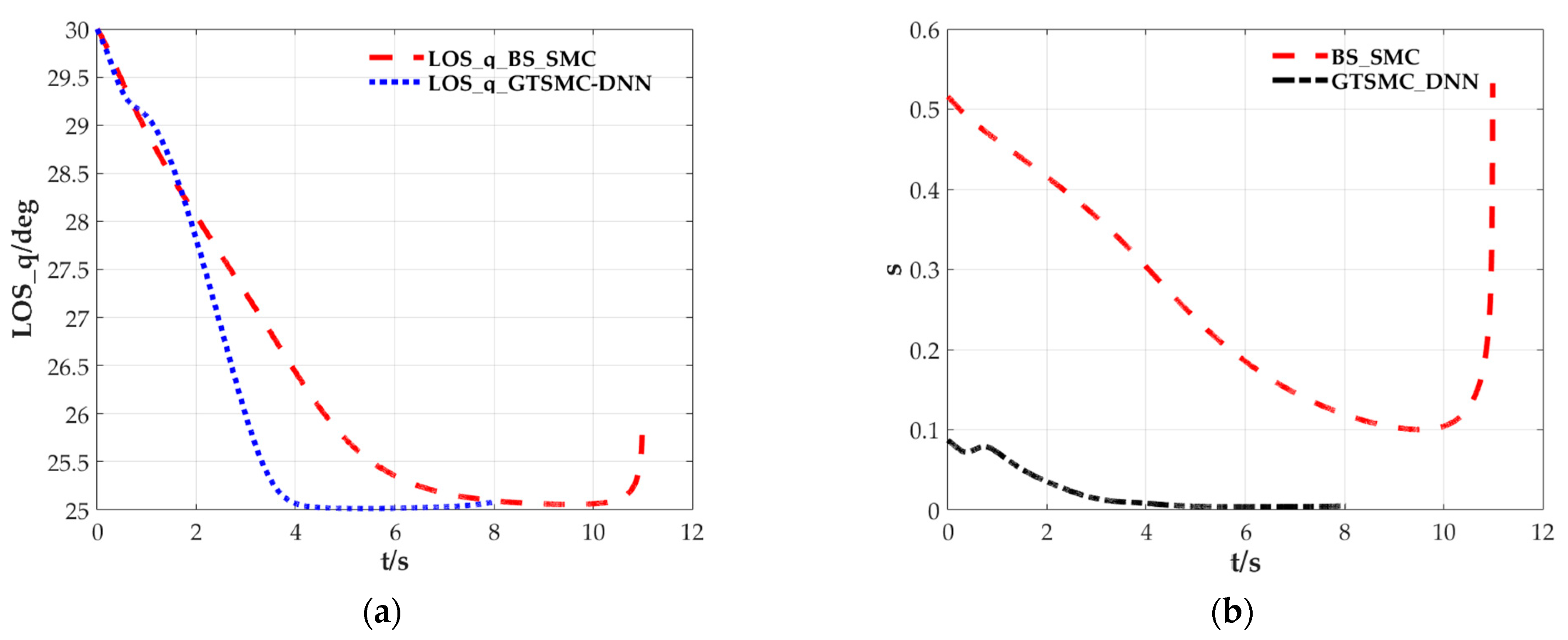
Figure 10a,b gives the variation of LOS angle and the sliding mode surface. It is clear that the LOS angle can be converged to the desired angle earlier by using GTSMC-DNN method. This also verifies Remark 1 and the first design objective mentioned in Section 3.1. Additionally, although the LOS angle can also be converged to the desired angle by using the BS-SMC method, the LOS angle becomes divergent gradually, especially when approaching the target.
As shown in Figure 10b, it is clear that the sliding mode surface can converge to zero earlier and the amplitude is relatively small when using GTSMC-DNN. This design objective is mentioned in Section 3.1. By extension, the reason why the surface has a small error nearing zero may be because the target is in a consistent state of maneuvering.
Figure 11 gives the variation of the adaptive weight parameters of DNN and the trajectory inclination angle. It is obvious that the amplitude of is relatively smaller when using GTSMC-DNN. Additionally, the system state curves change more violently when using the BS-SMC method, which verifies the second design objective mentioned in Section 3.1. As shown in Figure 11a, it is clearly that the adaptive weight parameters of DNN gradually converge to a fixed value. Thus, all these phenomena show that using the GTSMC-DNN method proposed in this paper can have a better control performance, which can also verify the design objectives mentioned in Section 3.1.
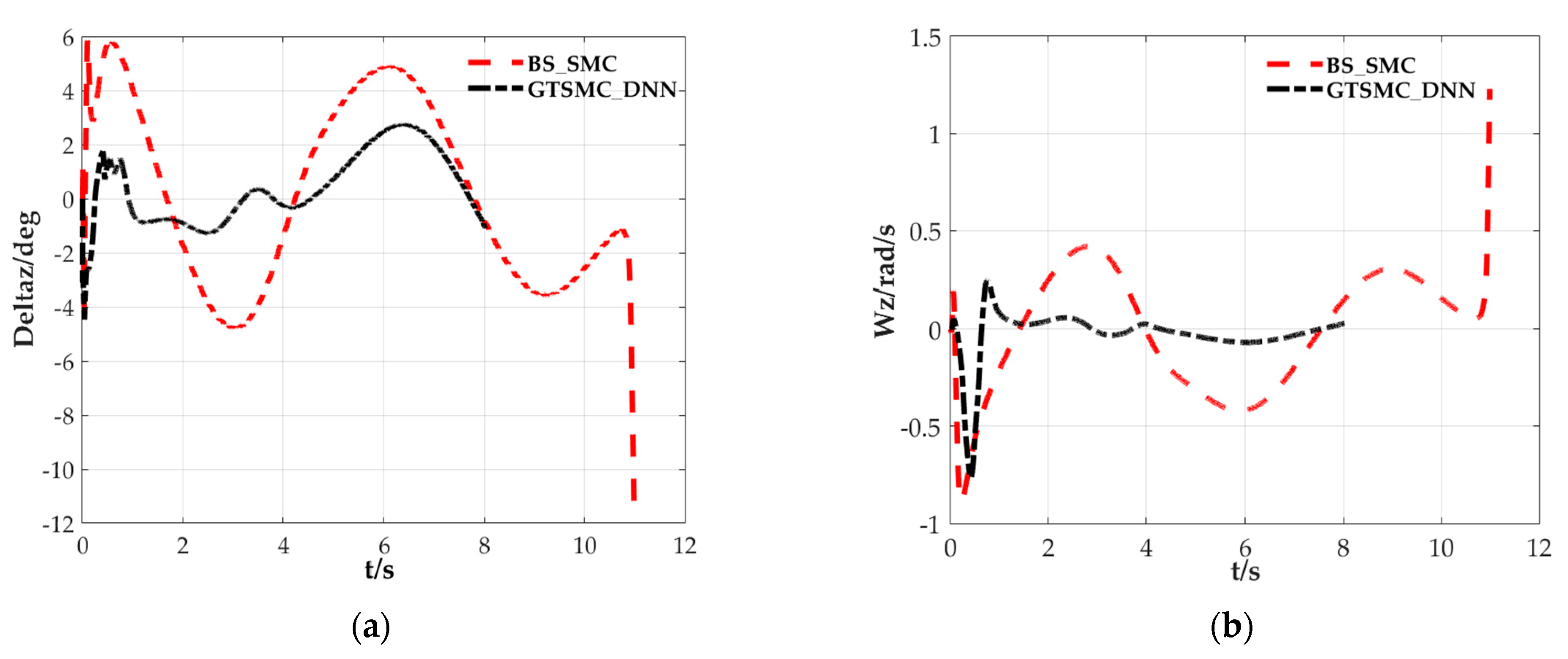
Figure 12 shows the variation of the rudder deflection angle and the pitch angular rate. It is clear that the rudder deflection angle is relatively smoother, and the amplitude is smaller when using the GTSMC-DNN approach. This demonstrates that using the GTSMC-DNN approach can have a better control performance. In addition, Figure 11b shows the variation of the pitch angular rate. Compared with the BS-SMC method, the amplitude of the pitch angular rate is relatively smaller and smoother. Furthermore, the convergence speed of the rudder deflection angle and the pitch angular rate is relatively faster by using GTSMC-DNN.
Thus, using GTSMC-DNN can have a better control performance under case I condition, which also verify the design objectives mentioned in Section 3.1.
5.2. Case II
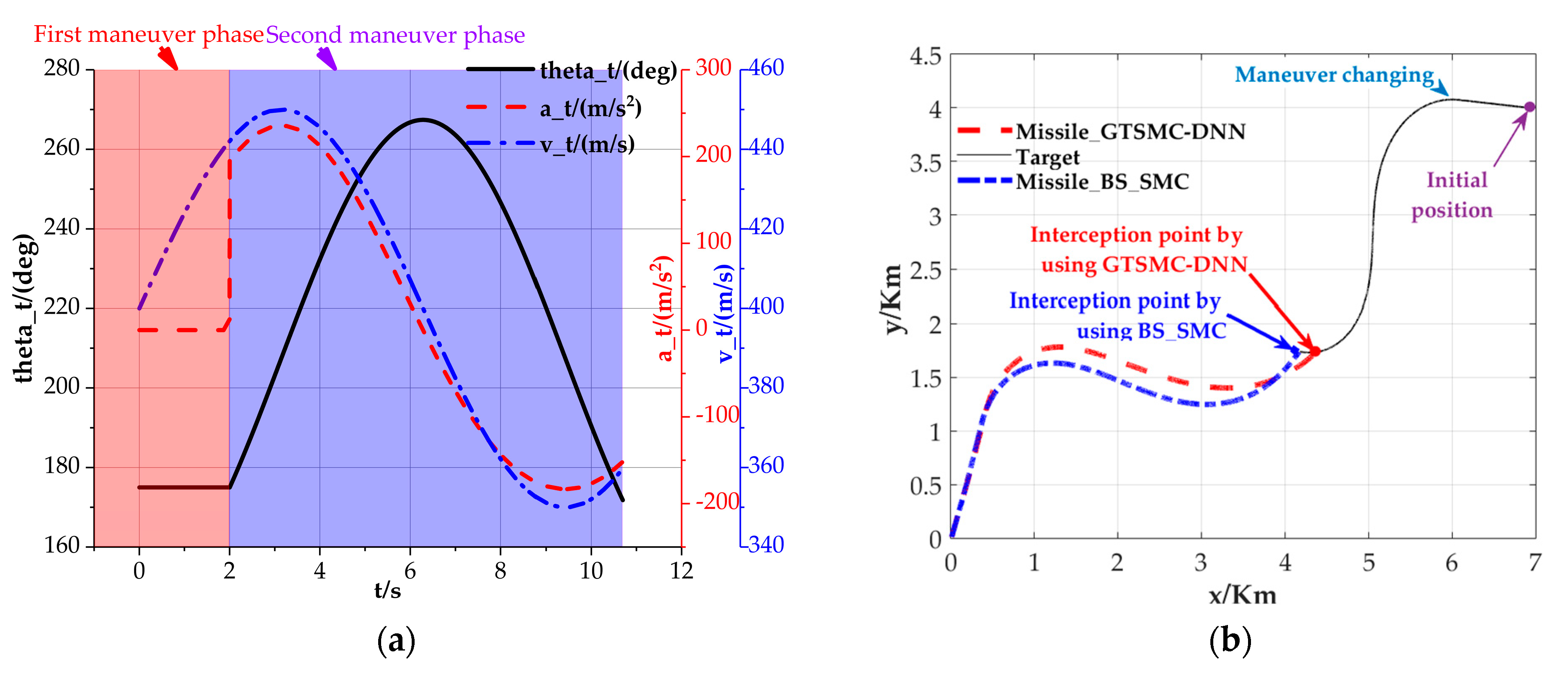
In this case, the missile will intercept a target with two maneuvering modes. During the first phase, the maneuvering target satisfies , and, after 2 s, the maneuvering target satisfies . The simulation results are shown in Figure 13, Figure 14, Figure 15 and Figure 16.
Figure 13 presents the maneuverability of the target and the trajectory of the missiles and the target. In Figure 13a, it is clear that the target adopts variable maneuvering speeds before 2 s, while the target suddenly takes a large-angle maneuver at 2 s. Even so, the missile can still intercept the target. In terms of interception time, the missile can intercept the target earlier by using the GTSMC-DNN method, which can also verify the design objectives mentioned in Section 3.1.
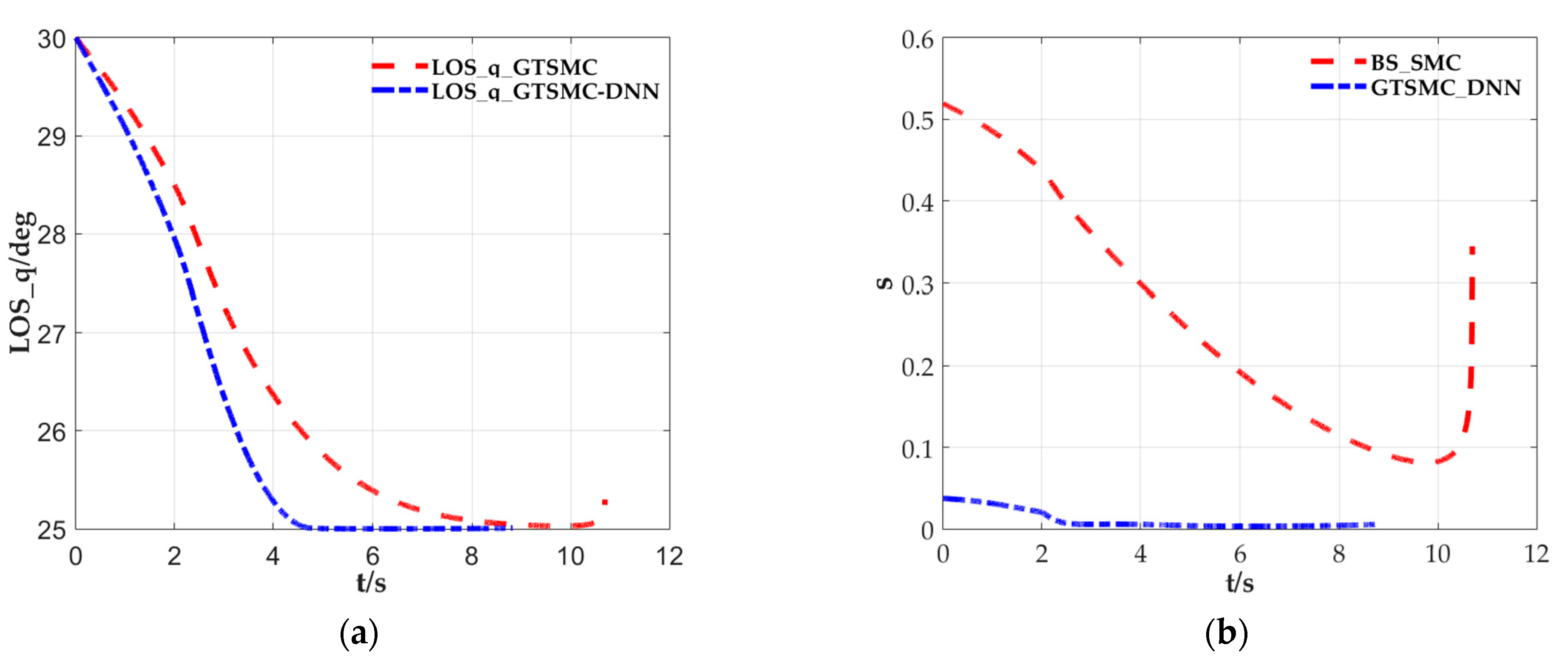
Figure 14a,b shows the system states of LOS angle and the variation of the sliding mode surface. It is obvious that the LOS angle can also be converged to the desired angle earlier, using the GTSMC-DNN method. This also verifies Remark 1, and the first design objective mentioned in Section 3.1.
Figure 15 shows the variation of the system state for the trajectory inclination angle and the adaptive weight parameters of DNN. It is clear that the amplitude of is relatively smaller and the variation is more advanced. This also reflects that the method proposed in this paper has a strong predictability and adaptability. In Figure 15a, we can also perceive that with the target changing the maneuvering mode suddenly at 2 s, the adaptive weight parameters of DNN exhibit a slight fluctuation. However, it can also be soon converged. Therefore, all this illustrates the second and third design objective mentioned in Section 3.1.
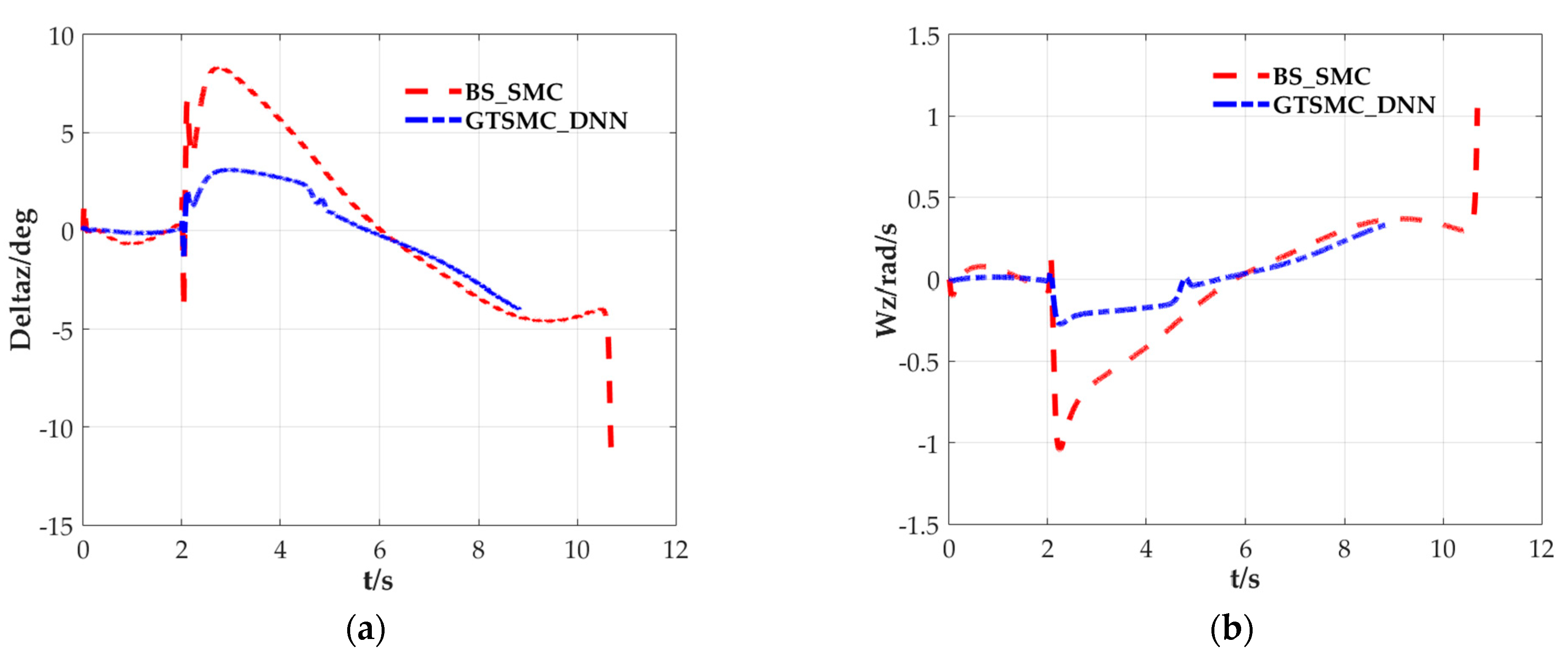
Figure 16 shows the variation of the rudder deflection angle and the pitch angular rate by using these two methods. It is clear that using the GTSMC-DNN approach, the amplitude of the rudder deflection angle is smaller. In addition, Figure 16b shows the variation of the pitch angular rate. Compared with the BS-SMC method, the amplitude of the pitch angular rate is relatively smaller and smoother.
Thus, under case II conditions, using the GTSMC-DNN method proposed in this paper can show a better control performance, which can also illustrate the design objectives mentioned in Section 3.1.
5.3. Case III (Monte Carlo Simulations)
In this section, the paper will demonstrate the robustness of the IGC system and introduce the Monte Carlo simulation. The uncertain disturbances will also be added into the system. In addition, the other conditions are listed in Table 4.
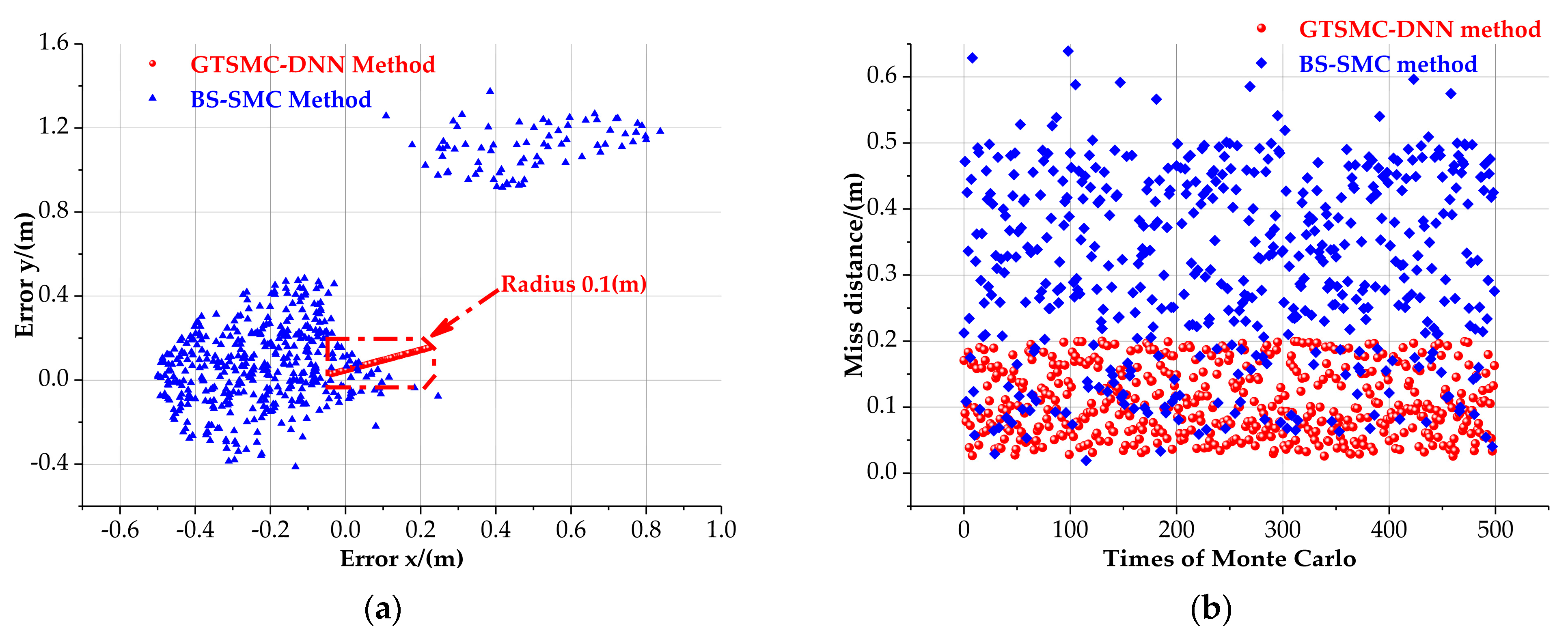
The simulation result is presented in Figure 17.
As shown in Figure 17a, it is obvious that compared with the BS-SMC method, the missile impacting points are relatively concentrated. By extension, most impacting points of the GTSMC-DNN method are relatively smaller and the impacting radius is about 0.1 m.
Figure 17b provides the miss distance for each time. It is obvious that all these impacting points are less than 0.2 m, using the GTSMC-DNN method. This also reflects that the method has a higher interception accuracy.
Thus, according to all the simulation results under different conditions, using the GTSMC-DNN method proposed in this paper can have a better interception performance, which also verifies all design objectives mentioned in Section 3.1.
6. Conclusions
To improve the performance in intercepting the target with different maneuvering modes and changing the mode suddenly during the interception, a new control algorithm for the IGC system is proposed by combining the GTSMC (Global Terminal Sliding Mode Control) method, the SOF (Second Order Filter) and the DNN (Deep Neural Network). After formulating the missile–target problem, the paper establishes the fourth-order IGC dynamic model with uncertain items. To truly reflect the characteristics of uncertainty, the paper establishes the uncertain equations. Then, the IGC system is divided into four subsystems, including the guidance subsystem, the overload subsystem, the attitude subsystem and the deep neural network subsystem. To transform the virtual control signal between each subsystem, the paper defines the SOF. Then, combined with the DNN, SOF and the GTSMC method, a new modified sliding mode surface and the reaching law are designed to obtain the adaptive control law. Then, the paper proves the stability of the system by using Lyapunov’s theory. Finally, several simulation cases are provided to demonstrate the superiority of the proposed method in improving the adaptive interception capability, increasing the control performance and having a high interception accuracy. In the future, several directions can be researched, such as researching the control performance with different layers and more neurons in 6DoF, verifying the control performance by using DNN only and others. In addition, another direction that uses the DNN to accomplish the autonomous target replacement can also be a research point. In conclusion, there are many other more interesting research directions.
Author Contributions
Conceptualization, J.Y; Methodology, K.N., X.B., X.C., J.L. and J.Y.; Software, K.N. and X.B.; Validation, X.C. and D.Y.; Formal analysis, K.N., X.B., X.C. and J.Y.; Investigation, X.B. and D.Y.; Data curation, K.N., X.C. and D.Y.; Writing – original draft, K.N., X.B. and J.L.; Writing – review & editing, X.C., D.Y., J.L. and J.Y. All authors have read and agreed to the published version of the manuscript.
Funding
The authors are grateful for the support of the National Natural Science Foundation of China (No. 61673212).
Data Availability Statement
Not applicable.
Acknowledgments
The authors would like to thank the flight control lab of Beijing University of Technology for their support for this research.
Conflicts of Interest
The authors declare no conflict of interest.
References
- Niu, K.; Chen, X.; Yang, D.; Li, J.; Yu, J. A New Sliding Mode Control Algorithm of IGC System for Intercepting Great Maneuvering Target Based on EDO. Sensors 2022, 22, 7618. [Google Scholar] [CrossRef] [PubMed]
- Chen, S.W.; Wang, W.; Fan, J.F.; Ji, Y. Impact angle constraint guidance law using fully-actuated system approach. Aerosp. Sci. Technol. 2023, 136, 108220. [Google Scholar] [CrossRef]
- Guo, J.G.; Xiong, Y.; Zhou, J. A new sliding mode control design for integrated missile guidance and control system. Aerosp. Sci. Technol. 2018, 78, 54–61. [Google Scholar] [CrossRef]
- Santoso, F.; Garratt, M.A.; Anavatti, S.G. State-of-the-art integrated guidance and control systems in unmanned vehicles: A Review. IEEE Syst. J. 2021, 15, 3312–3323. [Google Scholar] [CrossRef]
- Wang, Y.; Wang, H.; Lin, D.; Wang, W. Nonlinear Guidance Laws for Maneuvering Target Interception With Virtual Look Angle Constraint. IEEE Trans. Aerosp. Electron. Syst. 2021, 58, 2807–2822. [Google Scholar] [CrossRef]
- Dong, M.; Xu, X.; Xie, F. Constrained Integrated Guidance and Control Scheme for Strap-Down Hypersonic Flight Vehicles with Partial Measurement and Unmatched Uncertainties. Aerospace 2022, 9, 840. [Google Scholar] [CrossRef]
- Tian, Y.T.; Jing, W.X.; Gao, C.S.; An, R. Adaptive improved super-twisting integral sliding mode guidance law against maneuvering target with terminal angle constraint. Aerosp. Sci. Technol. 2022, 129, 107820. [Google Scholar]
- Garone, E.; Di Cairano, S.; Kolmanovsky, I. Reference and command governors for systems with constraints: A survey on theory and applications. Automatica 2017, 75, 306–328. [Google Scholar] [CrossRef]
- Li, X.; Chen, W.; Chen, Z.; Wang, T.; Shi, H. Fixed-Time Circular Impact-Time Guidance with Look Angle Constraint. Aerospace 2022, 9, 356. [Google Scholar] [CrossRef]
- Ming, C.; Wang, X.; Sun, R. A novel non-singular terminal sliding mode control-based integrated missile guidance and control with impact angle constraint. Aerosp. Sci. Technol. 2019, 94, 105368. [Google Scholar] [CrossRef]
- Liu, W.; Wei, Y.; Duan, G. Barrier Lyapunov function-based integrated guidance and control with input saturation and state constraints. Aerosp. Sci. Technol. 2018, 84, 845–855. [Google Scholar] [CrossRef]
- Li, K.B.; Liao, X.P.; Liang, Y.G.; Li, C.Y.; Chen, L. Guidance strategy with impact angle constraint based on pure proportional navigation. Acta Aeronaut. Astronaut. Sin. 2020, 41, 79–88. [Google Scholar]
- Wang, C.; Dong, W.; Wang, J.; Shan, J. Nonlinear suboptimal guidance law with impact angle constraint: An SDRE-based approach. IEEE Trans. Aerosp. Electron. Syst. 2020, 56, 4831–4840. [Google Scholar] [CrossRef]
- Han, T.; Xi, Y.; Chen, G.; Hu, Q. Three-Dimensional Impact Time and Angle Guidance via Controlling Line-of-Sight Dynamics. In Proceedings of the 2020 Chinese Control and Decision Conference (CCDC), Hefei, China, 22–24 August 2020; pp. 2850–2855. [Google Scholar]
- Chen, Y.; Shan, J.; Liu, J.; Wang, J.; Xin, M. Impact time and angle constrained guidance via range-based line-of-sight shaping. Int. J. Robust Nonlinear Control 2022, 32, 3606–3624. [Google Scholar] [CrossRef]
- Zhang, W.; Chen, W.; Li, J.; Yu, W. Guidance algorithm for impact time, angle, and acceleration control under varying velocity condition. Aerosp. Sci. Technol. 2022, 123, 107462. [Google Scholar] [CrossRef]
- Hu, Q.; Han, T.; Xin, M. Sliding-Mode Impact Time Guidance Law Design for Various Target Motions. J. Guid. Control Dyn. 2019, 42, 136–148. [Google Scholar] [CrossRef]
- Hou, Z.; Yang, Y.; Liu, L.; Wang, Y. Terminal sliding mode control based impact time and angle constrained guidance. Aerosp. Sci. Technol. 2019, 93, 105142. [Google Scholar] [CrossRef]
- Ma, S.; Wang, X.; Wang, Z. Field-of-View Constrained Impact Time Control Guidance via Time-Varying Sliding Mode Control. Aerospace 2021, 8, 251. [Google Scholar] [CrossRef]
- Zhou, X.H.; Wang, W.H.; Liu, Z.H. Fixed-time cooperative guidance for multiple missiles with impact angle constraint. J. Aerosp. Eng. 2021, 236, 1984–1998. [Google Scholar] [CrossRef]
- Zhang, W.G.; Yi, W.J.; Guan, J.; Qu, Y. Three-dimensional impact angle guidance law based on robust repetitive control. SN Appl. Sci. 2019, 1, 1–7. [Google Scholar] [CrossRef]
- Kang, S.; Tekin, R.; Holzapfel, F. Generalized impact time and angle control via look-angle shaping. J. Guid. Control Dyn. 2019, 42, 695–702. [Google Scholar] [CrossRef]
- Tekin, R.; Erer, K.S.; Holzapfel, F. Impact Time Control with Generalized-Polynomial Range Formulation. J. Guid. Control Dyn. 2018, 41, 1190–1195. [Google Scholar] [CrossRef]
- Cao, L.F.; Cao, H.S.; Liu, P.F.; Liu, H.; Xiao, Y. Parameter optimization of proportional navigation guidance for 2D trajectory correction projectile with fixed canard. Acta Aeronaut. Astronaut. Sin. 2021, 42, 604–614. [Google Scholar]
- Wang, C.; Yu, H.; Dong, W.; Wang, J. Three-dimensional impact angle and time control guidance law based on two-stage strategy. IEEE Trans. Aerosp. Electron. Syst. 2022, 58, 5361–5372. [Google Scholar] [CrossRef]
- Li, H.; Wang, J.; He, S.; Lee, C.-H. Nonlinear optimal 3-d impact-angle-control guidance against maneuvering targets. IEEE Trans. Aerosp. Electron. Syst. 2021, 58, 2467–2481. [Google Scholar] [CrossRef]
- Lin, L.-G.; Xin, M. Missile guidance law based on new analysis and design of sdre scheme. J. Guid. Control Dyn. 2019, 42, 853–868. [Google Scholar] [CrossRef]
- Kumar, S.R.; Maity, A. Finite-horizon robust suboptimal control-based impact angle guidance. IEEE Trans. Aerosp. Electron. Syst. 2019, 56, 1955–1965. [Google Scholar] [CrossRef]
- Gaudet, B.; Furfaro, R.; Linares, R. Reinforcement learning for angle-only intercept guidance of maneuvering targets. Aerosp. Sci. Technol. 2020, 99, 105746. [Google Scholar] [CrossRef]
- Gong, X.; Chen, W.; Chen, Z. All-aspect attack guidance law for agile missiles based on deep reinforcement learning. Aerosp. Sci. Technol. 2022, 127, 107677. [Google Scholar] [CrossRef]
- Chen, Y.; Wu, S.; Wang, X.; Zhang, D.; Jia, J.; Li, Q. Time and FOV constraint guidance applicable to maneuvering target via sliding mode control. Aerosp. Sci. Technol. 2023, 133, 108104. [Google Scholar] [CrossRef]
- Chen, Y.; Wu, S.; Wang, X.L. Impact time and angle control optimal guidance with field-of-view constraint. J. Guid. Control Dyn. 2022, 45, 2369–2378. [Google Scholar] [CrossRef]
- Zhang, X.; Dong, F.; Zhang, P. A new three-dimensional fixed time sliding mode guidance with terminal angle constraints. Aerosp. Sci. Technol. 2022, 121, 107370. [Google Scholar] [CrossRef]
- Yang, B.; Jing, W.X.; Gao, C.S. Three-dimensional cooperative guidance law for multiple missiles with impact angle constraint. J. Syst. Eng. Electron. 2020, 31, 1286–1296. [Google Scholar]
- Guo, J.; Li, Y.; Zhou, J. A new continuous adaptive finite time guidance law against highly maneuvering targets. Aerosp. Sci. Technol. 2018, 85, 40–47. [Google Scholar] [CrossRef]
- Lee, S.; Cho, N.; Kim, Y. Impact-time-control guidance strategy with a composite structure considering the seeker’s field-of-view constraint. J. Guid. Control Dyn. 2020, 43, 1566–1574. [Google Scholar] [CrossRef]
- Guo, J.; Li, Y.; Zhou, J. Qualitative indicator-based guidance scheme for bank-to-turn missiles against couplings and maneuvering targets. Aerosp. Sci. Technol. 2020, 106, 106196. [Google Scholar] [CrossRef]
- Wang, X.; Lu, H.; Huang, X.; Yang, Y.; Zuo, Z. Three-dimensional time-varying sliding mode guidance law against maneuvering targets with terminal angle constraint. Chin. J. Aeronaut. 2021, 35, 303–319. [Google Scholar] [CrossRef]
- Dong, W.; Wang, C.; Wang, J.; Xin, M. Three-dimensional nonsingular cooperative guidance law with different field-of-view constraints. J. Guid. Control Dyn. 2021, 44, 2001–2015. [Google Scholar] [CrossRef]
- Lee, S.; Kim, Y. Capturability of impact-angle control composite guidance law considering field-of-view limit. IEEE Trans. Aerosp. Electron. Syst. 2019, 56, 1077–1093. [Google Scholar] [CrossRef]
- Hu, Q.; Cao, R.; Han, T.; Xin, M. Field-of-view limited guidance with impact angle constraint and feasibility analysis. Aerosp. Sci. Technol. 2021, 114, 106753. [Google Scholar] [CrossRef]
- Duvvuru, R.; Maity, A.; Umakant, J. Three-dimensional field of view and im-pact angle constrained guidance with terminal speed maximization. Aerosp. Sci. Technol. 2022, 126, 107552. [Google Scholar] [CrossRef]
Figure 1.
The target with different maneuver modes during the interception.

Figure 2.
Guidance geometry.

Figure 3.
Dynamics of the missile in the pitch plane.

Figure 4.
Structure of proposed approach.

Figure 5.
(a) Structure of deep neural network. (b) The structure of a neuron model.

Figure 6.
The structure of deep neural network used in the guidance subsystem.

Figure 7.
The structure of deep neural network used in overload subsystem.

Figure 8.
The structure of the deep neural network used in the attitude subsystem.

Figure 9.
(a) The maneuver characteristics of the target; (b) The missile-target pursuit trajectory.
Figure 9.
(a) The maneuver characteristics of the target; (b) The missile-target pursuit trajectory.

Figure 10.
(a) System states of LOS angle; (b) The sliding mode surface.

Figure 11.
(a) The adaptive weight parameters of DNN; (b) System states of angle.

Figure 12.
(a) System states of angle; (b) System states of angle.

Figure 13.
(a) The maneuver characteristics of the target; (b) The missile–target pursuit trajectory.
Figure 13.
(a) The maneuver characteristics of the target; (b) The missile–target pursuit trajectory.

Figure 14.
(a) System states of LOS angle; (b) The sliding mode surface.

Figure 15.
(a) The adaptive weight parameters of DNN; (b) System states of angle.

Figure 16.
(a) System states of angle; (b) System states of angle.

Figure 17.
(a) The distribution of the 500 intercept points; (b) The characteristic of the relative distance.
Figure 17.
(a) The distribution of the 500 intercept points; (b) The characteristic of the relative distance.


Table 1.
Parameters of GTSMC-DNN.
| kl | C3 | C2 |
|---|---|---|
Table 2.
Initial parameters of the missile and target.
| Item | Initial Value | Unit |
|---|---|---|
| m | ||
| m | ||
| deg | ||
| deg | ||
| m/s | ||
| m/s | ||
| deg | ||
| deg |
Table 3.
The miss distance and terminal LOS angle.
| Item | GTSMC-DNN | BS-SMC | Unit |
|---|---|---|---|
| Miss distance of M-T | 0.257 | 2.207 | m |
| Terminal LOS | 25.126 | 25.754 | deg |
Table 4.
The Monte Carlo parameters under case III.
| Symbol | Quantity | Values |
|---|---|---|
| flight path angle of missile | ||
| LOS | ||
| velocity of the missile | ||
| the rate of pitch angle | ||
| Initial position in x | ||
| Initial position in y | ||
| pitch angle | ||
| Initial position in x | ||
| Initial position in y | ||
| velocity of the T | ||
| flight path angle of T | ||
| acceleration of T | ||
| rudder deflection |
Disclaimer/Publisher’s Note: The statements, opinions and data contained in all publications are solely those of the individual author(s) and contributor(s) and not of MDPI and/or the editor(s). MDPI and/or the editor(s) disclaim responsibility for any injury to people or property resulting from any ideas, methods, instructions or products referred to in the content. |
© 2023 by the authors. Licensee MDPI, Basel, Switzerland. This article is an open access article distributed under the terms and conditions of the Creative Commons Attribution (CC BY) license (https://creativecommons.org/licenses/by/4.0/).
Share and Cite
MDPI and ACS Style
Niu, K.; Bai, X.; Chen, X.; Yang, D.; Li, J.; Yu, J. A New Adaptive Control Algorithm of IGC System for Targets with Several Maneuvering Modes Based on GTSMC-DNN. Aerospace 2023, 10, 380. https://doi.org/10.3390/aerospace10040380
AMA Style
Niu K, Bai X, Chen X, Yang D, Li J, Yu J. A New Adaptive Control Algorithm of IGC System for Targets with Several Maneuvering Modes Based on GTSMC-DNN. Aerospace. 2023; 10(4):380. https://doi.org/10.3390/aerospace10040380
Chicago/Turabian StyleNiu, Kang, Xu Bai, Xi Chen, Di Yang, Jiaxun Li, and Jianqiao Yu. 2023. "A New Adaptive Control Algorithm of IGC System for Targets with Several Maneuvering Modes Based on GTSMC-DNN" Aerospace 10, no. 4: 380. https://doi.org/10.3390/aerospace10040380
Note that from the first issue of 2016, this journal uses article numbers instead of page numbers. See further details here.