
Studies of Satellite Position Measurements of LEO CubeSat to Identify the Motion Mode Relative to Its Center of Mass

Department of Space Research, Samara National Research University, 34 Moskovskoye shosse, 443086 Samara, Russia
*
Author to whom correspondence should be addressed.
Aerospace 2023, 10(4), 378; https://doi.org/10.3390/aerospace10040378
Submission received: 23 January 2023
/
Revised: 4 April 2023
/
Accepted: 12 April 2023
/
Published: 18 April 2023
(This article belongs to the Special Issue Optimal Spacecraft Planning and Control)
Abstract
:Highlights
- Study of LEO CubeSat dynamics using satellite position measurements.
- Refinement of ballistic coefficient using satellite position measurements of close-flying CubeSats.
Abstract
This paper addresses the possibility of reconstructing motion relative to the center of mass of a low Earth orbit (LEO) nanosatellite of the CubeSat 3U standard using satellite position measurements (Two-Line Element Set (TLE)). This kind of task needs to be performed in the case where it is not possible to establish radio communication with the nanosatellite after it is launched into orbit. Therefore, it is important for the nanosatellite developers to develop some understanding of what is going on with the nanosatellite in order to be able to analyze the current situation after deployment. The study was carried out on the example of the aerodynamically stabilized SamSat-218D nanosatellite developed by the professors and students of Samara National Research University. SamSat-218D was launched into a near-circular orbit with an average altitude of 486 km on April 2016 during the first launch campaign from the Vostochny cosmodrome. Knowledge of CubeSat aerodynamics allows estimating the nature of its possible motion relative to the CubeSat center of mass by ballistic coefficient changes, evaluated with the use of satellite position measurements. The analysis showed that SamSat-218D performed spatial rotation with an angular velocity of more than two degree per second and had not stabilized aerodynamically by 2 March 2022, when it entered the atmosphere and was destroyed.
1. Introduction
Nowadays there is a large number of CubeSats launched into low Earth orbits (LEO) [1,2], often via piggyback launches [3,4,5,6]. Usually, only 60% of CubeSat launches are successful [7,8,9,10]. Therefore, in a situation where the ground controllers are unable to contact the CubeSat, they can conduct a passive experiment to estimate CubeSat motion relative to its center of mass using NORAD Two-Line Element Sets (TLE) data [11].
CubeSats in LEO are affected by the following major torques: gravity gradient, aerodynamic, solar radiation, and magnetic torques. Taking into consideration the fact that the number of 3U CubeSat launches is more than 40% of the total number [12], the aerodynamic torque can often be used as a restoring one for them due to the increased static stability margin [13,14]. Reference [15] shows the regions where the influence of the main environmental torques prevail (Table 1). However, due to the design features of CubeSats, the boundary between regions 1 and 2 rises to 450 km (valid for 10% of static stability margin for 3U CubeSat with 0.3 m reference length), as shown in [13,16].
Some important features of the nanosatellite existence in low orbits are discussed in [16,17]: (i) Due to the aerodynamic torque, the angular acceleration of a nanosatellite is much greater than that of a satellite with larger dimensions and mass (for the same values of the relative static stability margin and bulk density). This expands the range of altitudes at which the aerodynamic torque acting on the nanosatellite is significant and can be used for passive stabilization along the velocity vector of the center of mass. (ii) The value of the ballistic coefficient of a nanosatellite is higher than that of a satellite with larger dimensions and mass (with the same bulk density), which leads to a decrease in its lifetime in orbit. It makes it possible to use LEO effectively and avoid clogging of near-Earth space. (iii) The value of the ballistic coefficient of a nanosatellite substantially depends on its orientation. The ratio of the maximum value of a 3U CubeSat ballistic coefficient to the minimum value is 4.75. This fact makes it possible to gain information about the CubeSat attitude and dynamics from the ballistic coefficient. Table 2 compares the main features of CubeSats discussed above.
Estimation of CubeSat motion relative to the center of mass using satellite position measurements is conceptually similar to the approaches applied to the development and refinement of atmospheric density assimilation models. However, in our study, we needed to know the atmospheric density in order to estimate the ballistic coefficient.
In this paper, it is important to note that the atmosphere is affected by solar and geomagnetic activities, meaning that the existing models of the atmosphere [18,19,20,21,22,23,24] differ from the actual atmosphere by 10–30% or more, as shown in [25]; therefore, atmospheric models require refinement based on real orbital data.
Existing empirical atmospheric models are formed and complemented by density estimation using satellite position measurements. Satellites carrying out such measurements include Russian series of spherical satellites Pion [26], Atmospheric Neutral Density Experiment (ANDE) [27], Drag and Atmospheric Neutral Density Explorer (DANDE) [28,29], SpinSat [30], Chinese spherical microsatellite [31], and QB50 missions [32,33].
Atmospheric density estimation is performed using mass spectrometers [34,35,36], accelerometers [37,38,39], satellite position measurements (obtained by GPS, TLEs) [39,40,41], and satellite laser ranging (SLR) [42] from Earth.
As an example, satellite position measurements in the form of TLE files were used in [43] to correct the thermosphere model. The main disadvantage of such data is the low time resolution of TLE files––1–3 measurements per day––with an accuracy of 100–200 m [44]. It is possible to use TLE files, where the data are averaged over a certain interval. In this way the authors of the study [45] estimated and analyzed the space debris ballistic coefficients using a large number of TLE files.
In the case that several CubeSats are launched as a piggyback payload, if at least one of them has a known value of ballistic coefficient and parameters of motion relative to the center of mass, this CubeSat can be considered as a reference satellite. Then, it is admissible to conduct an experiment to reconstruct the motion parameters relative to the CubeSat center of mass via satellite position measurements based on a priori information about the reference satellite.
In this paper, we propose a method for solving the inverse problem of a CubeSat ballistic coefficient estimation using the refined density of the atmosphere. The new method has two main components: (i) the study of CubeSat ballistic coefficient value changes; and (ii) the identification and study of the most probable nanosatellite motion relative to the center of mass based on the design features of CubeSats.
The method described in this paper is close to those reported in [17,46], which present a comprehensive analysis of the SamSat-218D ballistic coefficient variation during its first 100 days in the Earth orbit. In these papers, AIST-2D was considered as a reference satellite as long as both of them shared the same orbit. Reference [47] discusses the results obtained for the changes in the SamSat-218D nanosatellite ballistic coefficient during its five-year orbiting period. The consideration of the Chinese Tianwang constellation as an additional reference satellite along with AIST-2D made it possible to increase the reliability of the results obtained.
As a logical continuation of the work [47], the present study generalizes and refines the previously obtained results; in addition, for the first time, it presents the results of the study on ballistic coefficient changes throughout the satellite lifetime in orbit from the launch to the moment it reentered Earth’s atmosphere and was subsequently destroyed, which occurred approximately on 2 March 2022.
2. Problem Formulation
We consider a common situation: a group of satellites including CubeSats are launched into similar orbits as piggyback payloads. One of the satellites has an attitude determination and control system, and its mean ballistic coefficient is known. We consider this satellite as a reference one, and the CubeSat of interest to us will be henceforth referred to as a “considered” CubeSat. Moreover, it should be noted that the satellite position measurements of all satellites that we used are represented as TLE files.
After the launch of the satellite group into orbit, it is possible to use the known ballistic coefficient of the reference satellite to refine the atmospheric density, and these data are used to estimate the ballistic coefficient of the considered CubeSat.
Assuming that the CubeSat ballistic coefficient exceeds that of the reference satellite, within 2–3 months after the launch, the difference between the atmospheric layers in which both satellites are orbiting the Earth is growing, which requires the adjustment of the atmospheric density. As an example of such an adjustment, the State Technical Standard for atmospheric density (GOST 25645.101-83: Earth upper atmosphere. Density model for project ballistic computations of artificial Earth satellites) was used in [45,46] to adjust the atmospheric density to the relevant altitude, and in [47], the authors describe the use of the atmospheric model NRLMSISE-00 as a reference. In the present work, we also used NRLMSISE-00 model for similar adjustments.
When considering a short time interval (the first 100 days), we do not need to correct the atmosphere, instead, we can use the density values determined from the ballistic coefficient and position measurements of the reference satellite sharing the same orbit. On a longer study interval, when the satellite orbit heights do not differ much, it is acceptable to use a simple model to correct the atmosphere [45,46]. With a significant difference in satellite orbit heights, it is necessary to use a dynamic model of the Earth’s atmosphere, as proposed in [47].
With the further divergence of atmospheric layers, it is advisable to involve satellite position measurements from 1U CubeSats flying in a close formation. Since they move mostly uncontrollably, their average ballistic coefficients can be calculated. Using these data, it is expedient to study the nature of the considered CubeSat motion within the same altitude region as for the reference satellites.
3. Data and Methods
The main operation in the current study is the calculation of orbital radius r derived from the TLE data [11] in the case of a circular orbit:
where a (km) is the semi-major axis; μ = 398,602 km3s−2 is the Earth’s gravitational parameter; and n (rev/day) is the mean motion.
Satellite orbit perturbations caused by the aerodynamic acceleration Φ for a circular orbit are described by the formula [15]:
where is the derivative of a radius-vector.
The aerodynamic acceleration Φ is expressed as:
where B (m2/kg) is the ballistic coefficient; ρ is the atmospheric density; and v = (μ/r)0.5 (km/s) is the satellite velocity in the case of a circular orbit.
Using Equations (2) and (3), the ballistic coefficient is calculated as:
Motion relative to the mass center can be represented as the spatial rotation of the body frame Oxyz relative to the orbital frame OXYZ.
In the orbital frame OXYZ, center O coincides with the CubeSat mass center, the OZ axis is directed from the Earth center OE in the direction of the radius-vector r, the OY axis is coaxial with the direction of the vector of the true anomaly derivative, and the OX axis complements the orbital coordinate system to the right one.
In the body frame Oxyz, center O coincides with the CubeSat mass center, Ox is the longitudinal axis, and Oy and Oz are transversal axes. The axes are chosen in such a way that the main moments of inertia of the CubeSat satisfy relation Jx ≤ Jy ≤ Jz.
The Euler angles are used here to represent Oxyz attitude relative to OXYZ:
- -
- ψ (precession angle) is a signed angle between the OY axis and the OX × Ox unit vector;
- -
- α (angle of attack) is the angle between the longitudinal axis Ox and the velocity vector (OX axis for a circular orbit); and
- -
- φ (proper rotation angle) is a signed angle between the OX × Ox unit vector and the Oy axis.
We predicted orbital motion between two ephemerides with a simplified perturbation model SGP4 [48] along with the Runge-Kutta method (RK4) for numerical integration [49], taking into account only gravitational acceleration. These satellite position measurements are used to calculate atmospheric density by an empirical global reference atmospheric model of the Earth NRLMSISE-00 [23] in each point of orbit with a 60-s step. To calculate the derivative of the orbital radius, we used the smoothing spline method [50] and the finite difference method [49] coherently.
To estimate the possible modes of CubeSat motion relative to the center of mass, we used an approximate model of the angular motion of a dynamically symmetric CubeSat in the plane of a circular orbit relative to the trajectory coordinate system, which describes the changes in the angle of attack caused by the gravitational and aerodynamic restoring torques [51]:
where a(H) = a0Slρv2/(2Jx) is the coefficient due to the aerodynamic recovery moment; c(H) = 3(Jx − Jtr)μ/(2r3Jx) is the coefficient due to the gravitational moment; H is a flight altitude; a0 is the coefficient for approximation by sinusoidal dependence of the aerodynamic recovery moment coefficient; l is a characteristic length; S is a characteristic area; Jx is a longitudinal main moment of inertia; and Jtr is a transversal main moment of inertia.
To clarify the general properties of the system of Equation (5), we used the phase plane method. The changes in the altitude of the circular orbit due to atmospheric drag are very slow, and when considering the angular motion of the CubeSat on one or several revolutions, we can take H = const. In this case, for Equation (5), the energy integral E0 takes the form:
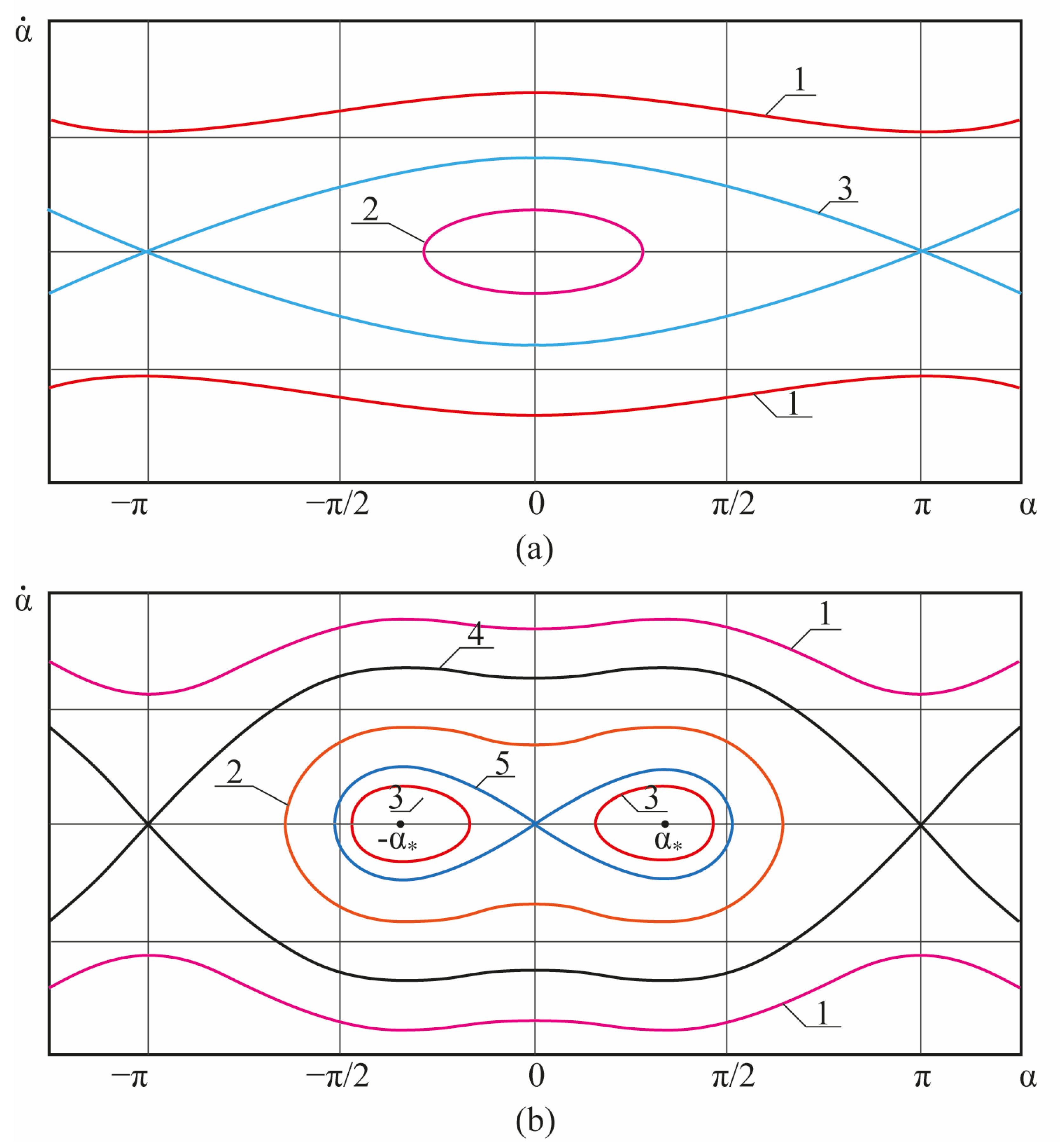
The nature of the CubeSat motion is determined by the ratio of the quantities a, c, and E0. In the case of a < 0, c > 0, there are two kinds of phase portraits: the first is (i) |a| ≥ 2c (aerodynamic torque is predominant). In this case, the CubeSat has two equilibrium positions for the angle of attack: stable with α = 0 + 2nπ (n = 0, ±1, ±2, …) and unstable with α = π + 2nπ (n = 0, ±1, ±2, …) (a schematic view of the phase portrait is shown in Figure 1a). The rotational motion mode of the CubeSat corresponds to the condition of E0 > −a + c (Figure 1a, phase trajectory 1) and the oscillatory motion mode relative to stable equilibrium α = 0 + 2nπ (n = 0, ±1, ±2, …) corresponds to the condition of E0 < −a + c (Figure 1a, phase trajectory 2). The regions of possible motions are separated by a separatrix c (Figure 1a, phase trajectory 3). The second is (ii) c > 0.5|a| (gravitational moment is predominant). With this ratio, there are four regions of the CubeSat motion: a rotational region and three oscillatory regions (a schematic view of the phase portrait is shown in Figure 1b). The CubeSat has four equilibrium positions for the angle of attack: α* = ±arccos (−0.5a/c) + 2nπ (n = 0, ±1, ±2, …), α = 0 + 2nπ (n = 0, ±1, ±2, …), and α = π + 2nπ (n = 0, ±1, ±2, …). The CubeSat rotational motion mode corresponds to the condition of E0 > −a + c (Figure 1b, phase trajectory 1); the oscillatory motion mode relative to the equilibrium position α = 0 + 2nπ (n = 0, ±1, ±2, …) corresponds to the condition of −a + c < E0 > a + c (Figure 1b, phase trajectory 2); and the oscillatory motion mode relative to the equilibrium position α* corresponds to the condition of E0 < a + c (Figure 1b, phase trajectory 3). The regions of possible motion modes are separated by separatrices (Figure 1b, phase trajectories 4 and 5).
4. Method for Identification of the CubeSat Motion Mode Relative to the Mass Center
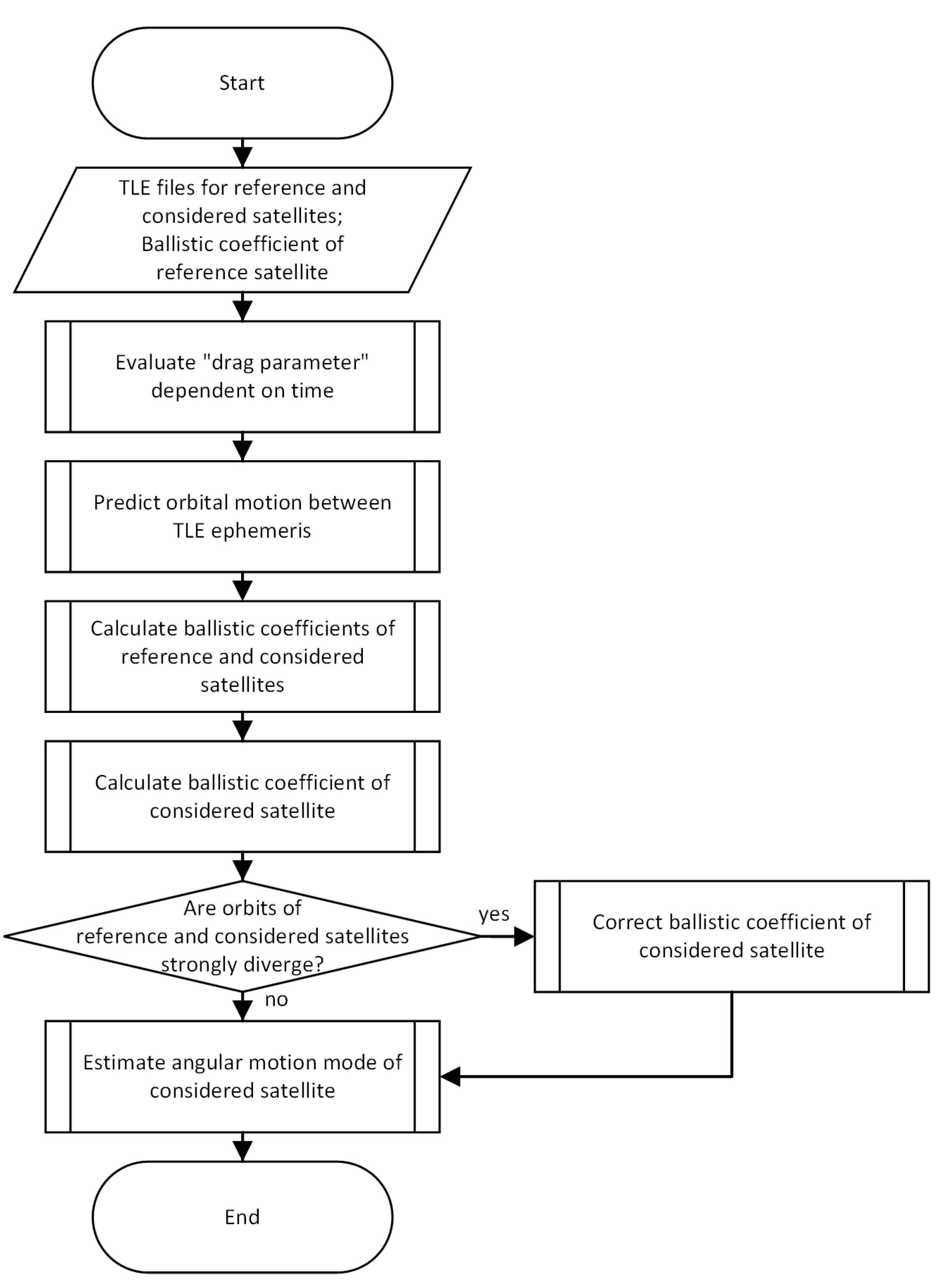
The main idea of indirect determination of the motion nature relative to the CubeSat center of mass is to apply data on the variable ballistic coefficient of the considered CubeSat to the entire research interval. In order to achieve this goal, we propose the method for estimating the CubeSat ballistic coefficient using satellite position measurements (Figure 2).
The method includes the following steps:
(1) Calculation of the radius-vectors using the satellite position measurements represented as TLE files for the reference and considered satellites as in Equation (1). Smoothing by a cubic smoothing spline with smoothing parameter p = 0.95 (selected value provides an acceptable interpolation with the removal of high-frequency noise) and re-discretization with time step Δt equal to one day of the radius-vector data of the reference and considered satellites. Calculation of the radius-vector derivative for the reference and considered satellites. Calculation of the “drag parameter” Di (here it is just a change of variables to further simplify calculations) for the reference and considered satellites:
where Δri/Δt is the numerical derivative of the radius vector.
(2) Prediction of orbital motion between TLE ephemeris. Calculation of the atmospheric density ρmodel in each point of orbit using the dynamic model NRLMSISE00. Averaging of ρmodel on each day:
(3) Calculation of the ballistic coefficient for the reference and considered satellites:
(4) In the case when the altitudes of the reference and considered satellites are close and the ballistic coefficient of the reference satellite is known as Bref, it is possible to calculate the density at the altitude of the reference satellite:
and the corrected ballistic coefficient of the considered CubeSat:
After substitution of Equation (10) into Equation (11), we obtain:
(5) In the case when the orbits of the reference and considered satellites strongly diverge, the ballistic coefficient of the considered CubeSat changes significantly (usually increases), which contradicts the physical sense. Then, we use the data of the other satellite, the one closest to the considered one and referred to as the second reference satellite. The ballistic coefficient of this satellite must be approximately constant. It is necessary to calculate the calibrated ballistic coefficient of the second reference satellite Bref2,cor using Equation (12), substituting the considered CubeSat for the second reference satellite.
While the altitudes of the considered and the second reference satellite are close, the changes in their ballistic coefficients have the same nature. For instance, the ballistic coefficients of the considered and the second reference satellites will constantly grow after step (5), when these two satellites are orbiting on much lower orbits than the reference satellite.
Then, the first-degree polynomial smoothing of the corrected ballistic coefficient of the second reference satellite is carried out using the least squares method [49]:
where aref2 is the slope coefficient or gradient of the line; bref2 is the B-intercept of the line.
Hence, we derive the corrected ballistic coefficient of the considered satellite by the formula:
(6) Study of the estimated ballistic coefficient to identify the motion mode relative to the center of mass. Here, we need to answer two questions: Does the ballistic coefficient have a constant value? Are there any stepped changes in the ballistic coefficient? The answers to these questions allow us to estimate the angular velocity of CubeSat and determine the motion mode, which will provide the information about conditions for CubeSat deployment into orbit.
5. Calculation
5.1. The First Launch from Vostochny
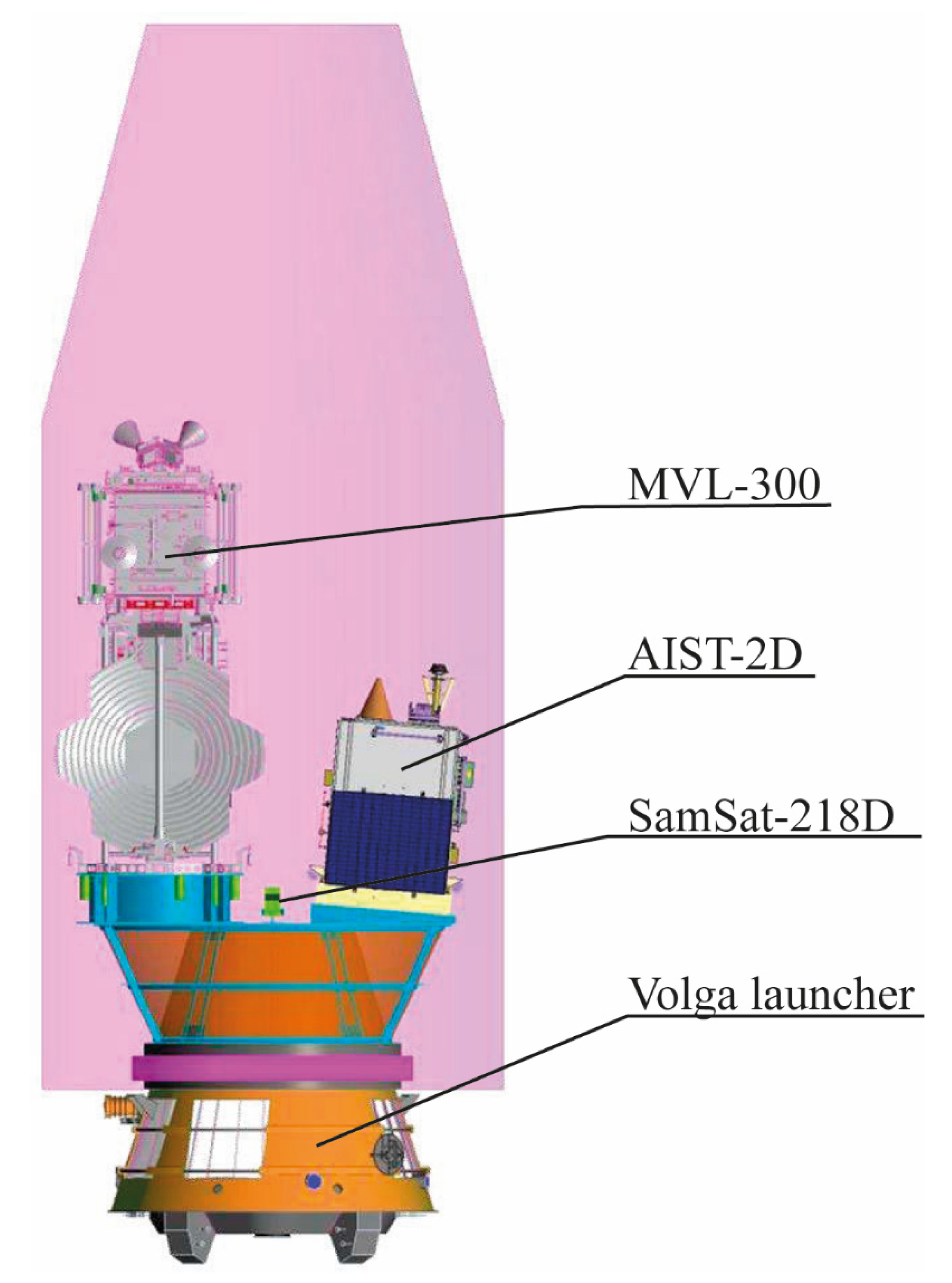
We verified the proposed method by studying the piggyback launch of 3U CubeSat SamSat-218D (Samara University, Samara, Russia) [53] together with satellites AIST-2D (Progress Rocket Space Centre, Samara, Russia) [54] and Lomonosov (Moscow State University, Moscow, Russia) [55] placed into orbit by the Soyuz-2.1a carrier rocket that started from the Vostochny Cosmodrome on April 28, 2016 [56]. Figure 3 shows all three satellites installed inside the payload fairing [57,58]. The initial altitude was 486 km; inclination was 97.3 deg; and eccentricity was 0.001.
The primary payload, Lomonosov or MVL-300, is an astrophysics research satellite. The Lomonosov project was initiated and carried out by Lomonosov Moscow State University. The main objective of the mission was the observation of gamma-ray bursts, high-energy cosmic rays and transient phenomena in the Earth’s upper atmosphere. Table 3 presents some of the main parameters of the satellite.
The second payload AIST-2D is an experimental small spacecraft developed jointly by engineers of the Rocket Space Center “Progress” (RSC Progress) and Samara State Aerospace University. AIST-2D was designed for Earth observation, as well as for scientific research [59]. The main parameters of the satellite are presented in Table 4.
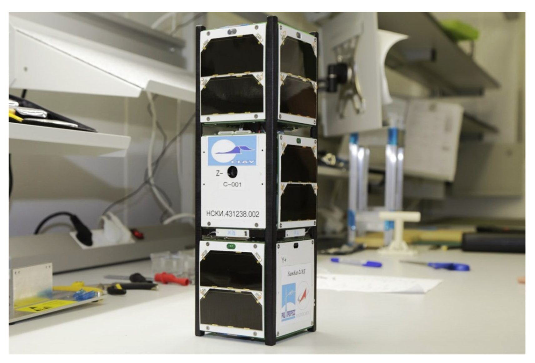
The third payload SamSat-218D (Figure 4) is the first nanosatellite designed by students and professors of Samara State Aerospace University to develop and test the technology of creating a closed-loop control for its spatial orientation with a large static stability margin. Table 5 presents the main parameters of the satellite.
5.2. Results and Discussion
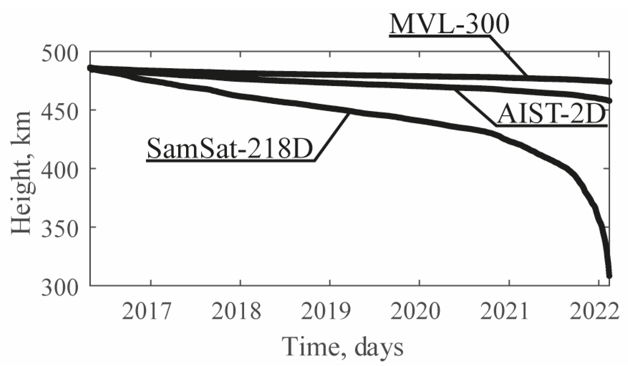
Figure 5 demonstrates the changes in the altitudes of satellite orbits within the time interval from 28 April 2016 to 2 March 2022. By the end of that period, the average altitude of SamSat-218D was 330 km.
We earlier discussed the first 100-day period of the SamSat-218D motion described in [45], where we suggested that the possible motion relative to the SamSat-218D center of mass within that period was transitional motion mode between different equilibrium positions of the angle of attack. Here, we consider the updated results based on the six-year SamSat-218D satellite position measurements.
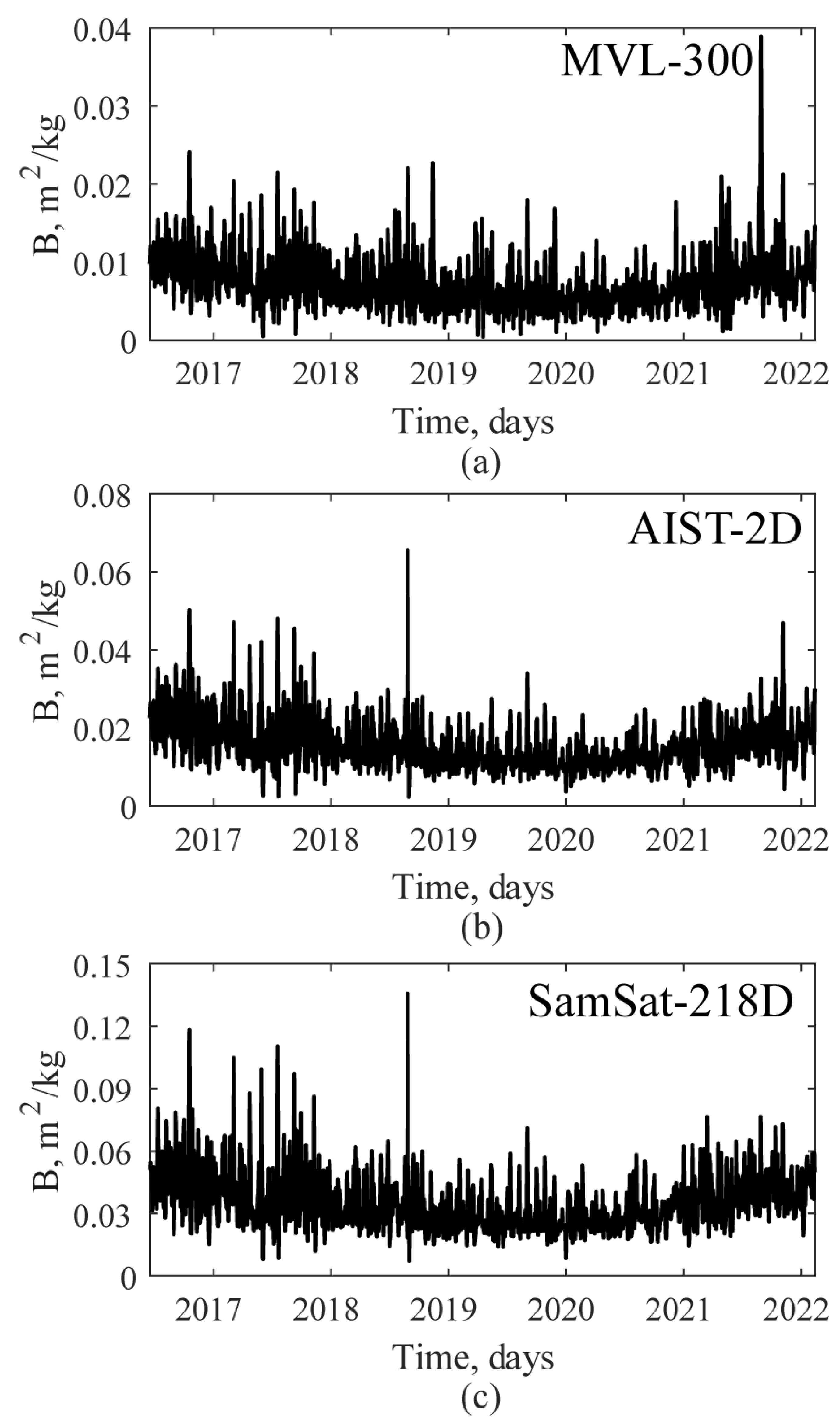
We used the first three steps of the proposed method in the processing of SamSat-218D, AIST-2D and MVL-300 data. Figure 6 demonstrates the results of the third step, namely, the ballistic coefficients estimated while accounting for the estimated drag data (satellite position measurements represented as TLE files) and the NRLMSISE-00 atmospheric density model. All these data series are highly correlated (correlation coefficient of MVL-300 Bmodel and AIST-2D satellites is 0.80; and the correlation coefficient of SamSat-218D Bmodel and AIST-2D satellites is 0.96). The noise in the plots of Figure 6 is due to the errors in the coordinates determined in the TLE file processing and the differences between the values of the model atmospheric density and the estimated one, caused by a short-period variation of solar activity.
Nevertheless, AIST-2D retained its orientation, and its ballistic coefficient is approximately constant (Bref = 0.0227 m2/kg). Therefore, we corrected the ballistic coefficient of SamSat-218D according to Step 4 (Figure 7). According to Step 5, the SamSat-218D ballistic coefficient was increasing and the slope coefficient of line smoothing aref2 = 3.51 × 10⁻⁶, which was caused by the increased difference in the atmospheric layers between the altitudes of AIST-2D and SamSat-218D.
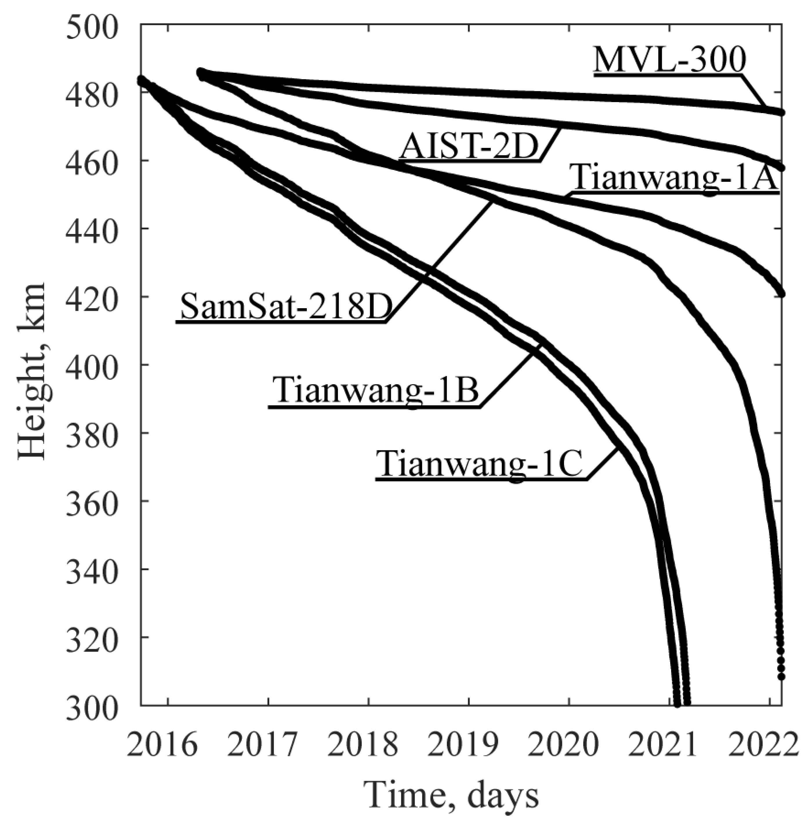
To correct the ballistic coefficient further, we used the data of the Chinese Tianwang constellation consisting of three CubeSats launched on 25 September 2015 [60]. Figure 8 demonstrates the altitudes of SamSat-218D, AIST-2D, and MVL-300 compared to Tianwang-1A, Tianwang-1B, and Tianwang-1C CubeSats.
Tianwang-1A is a 3U CubeSat with a 3-axis stabilized attitude determination and control subsystem and a micro-propulsion module. Tianwang-1B is a 2U CubeSat, with its main payload being an AIS receiver, to receive marine traffic information of the ground. Tianwang-1C is a standard 2U CubeSat with an ADS-B receiver as its main payload to monitor civilian aircraft flying within the nadir space region of the satellite. Apparently, owing to the attitude determination and control subsystem, Tianwang-1A was kept close to the aerodynamic equilibrium position, and despite a rather dense internal layout, its orbital lifetime was longer than those of the other two CubeSats from the joint launch. Tianwang-1B and Tianwang-1C must have been rotating uncontrollably until they deorbited. The fall in the SamSat-218D altitude is similar to the fall in the altitudes of Tianwang-1B and Tianwang-1C, which may be indicative of a similar nature of angular motion.
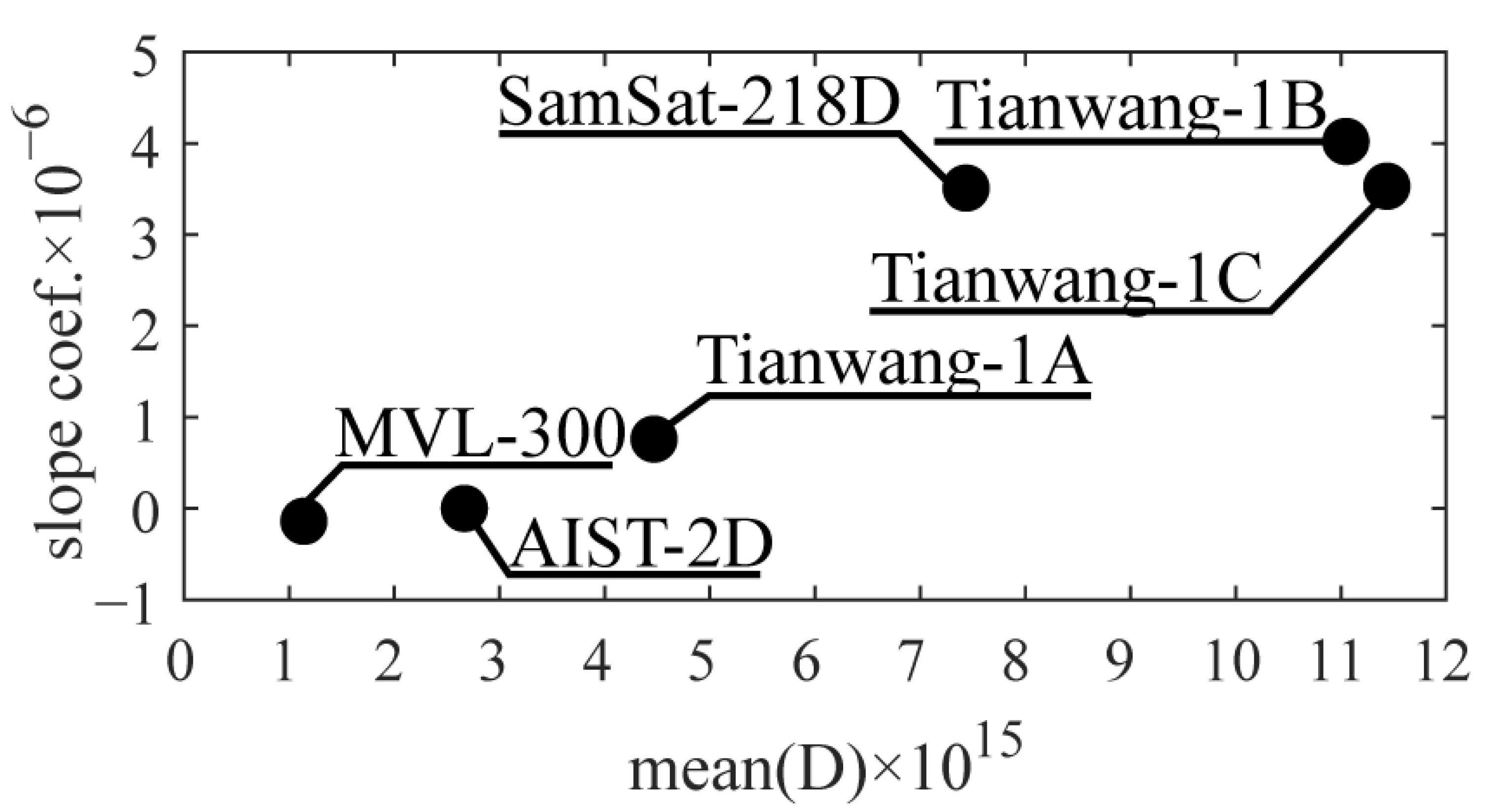
We calculated the corrected ballistic coefficients of six satellites (except AIST-2D) and approximated them by line polynomials. Figure 9 shows the dependency of the slope coefficient of the smoothed ballistic coefficient data on the mean drag coefficient. The slope coefficient of SamSat-218D was close to those of Tianwang-1B and Tianwang-1C. Therefore, we used the Tianwang-1C data for further correction of the coefficients at Step 5.
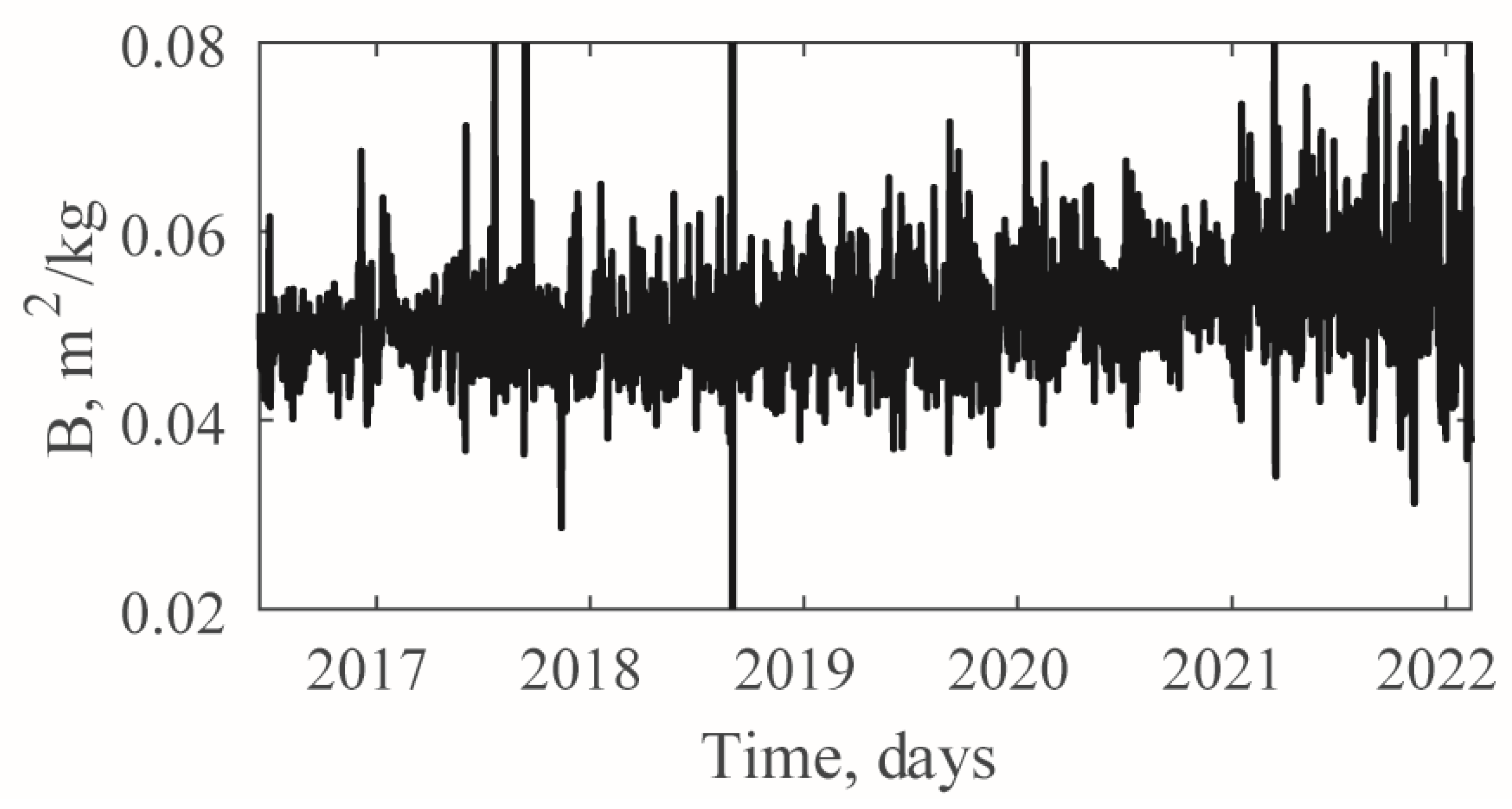
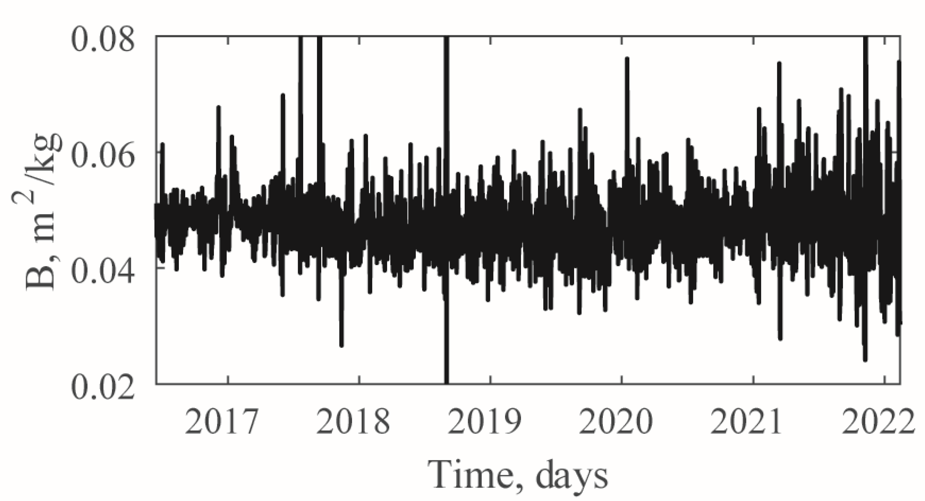
The results of the final correction of the SamSat-218D ballistic coefficient are shown in Figure 10. The mean ballistic coefficient is 0.047 m2/kg with the standard deviation of 0.013 m2/kg (such level of noise caused by the errors in determining the coordinates and the differences between the values of the model atmospheric density and the estimated one).
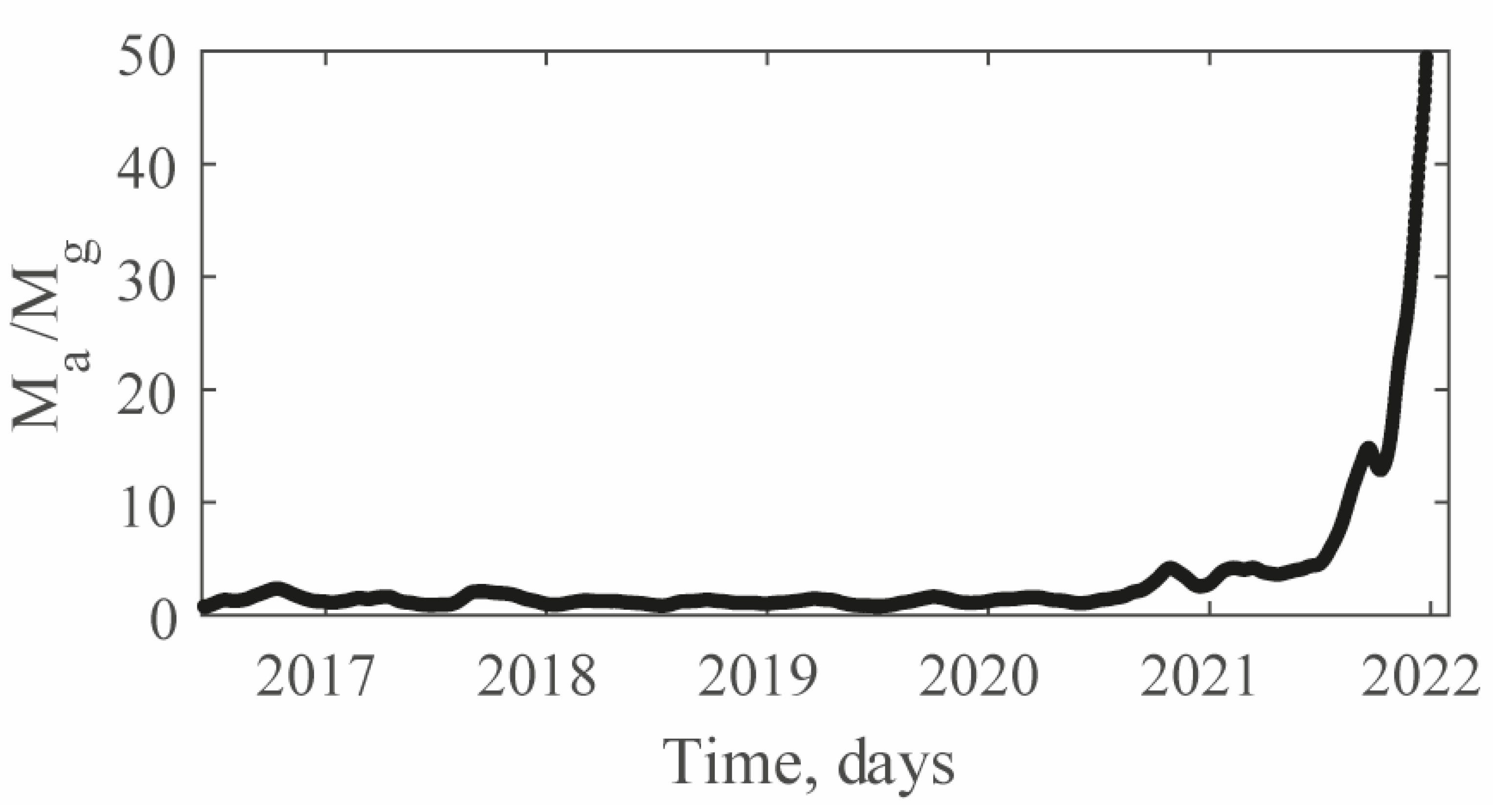
After the experimental estimation of the SamSat-218D ballistic coefficient, it was necessary to determine the nature of its angular motion. To do this, we estimated the ratio of the maximum aerodynamic moment to the maximum gravitational moment (it is equal to the ratio of |a(H)/c(H)| from Equation (5)) by simulating plane motion using the SamSat-218D altitude and average atmospheric density derived at the previous steps (Figure 11). The ratio obtained is indicative of the environmental conditions of SamSat-218D during the observation period.
The graph in Figure 11 can be divided into two time intervals:
(1) from the launch date to November 2020. It is characterized by comparable values of the gravitational and aerodynamic torques;
(2) from November 2020 to March 2022. This interval is noted by domination of aerodynamic torque caused by the decrease in the altitude and the increase in solar activity.
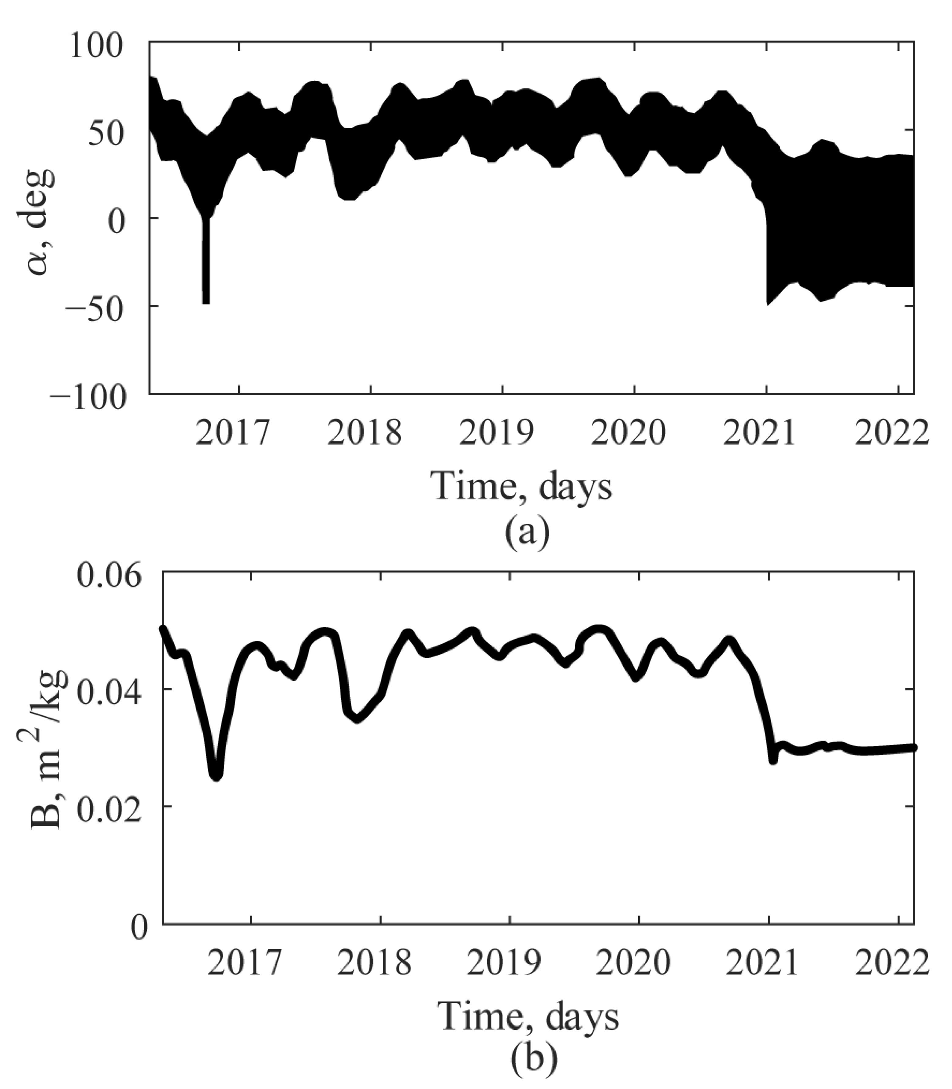
Taking into consideration the obtained ratio, we carried out a simulation using an approximate model of angular motion in the orbital plane, assuming a low angular velocity of 0.1 deg/s for the initial deployment angle of 80 deg (Table 5) and using a refined atmosphere in order to check whether the SamSat-218D motion was aerodynamically stabilized. Figure 12 shows the simulated angle of attack and the simulated time-dependent ballistic coefficient for this time interval.
The simulated ballistic coefficient is approximately equal to the experimental one within the time from the launch date to November 2020 (interval 1). The gravitational torque slightly exceeds the aerodynamic one, which causes oscillations relative to the equilibrium position. However, within the time from November 2020 to March 2022 (interval 2), the ballistic coefficient differs from the experimental one (Figure 10) due to the aerodynamic torque exceeding the gravitational torque and oscillations relative to the value of α = 0.
The coincidence of the simulated ballistic coefficient with the experimental one within time interval 1 is due to the fact that the density of the atmosphere remained practically unchanged. This is explained by the compensation for the decrease in altitude (leads to increase in density) under conditions of solar activity decrease (leads to decrease in density). As a result, the density value did not change very much. However, within interval 2, the divergence between the simulated (Figure 12b) and experimental (Figure 10) ballistic coefficients means that the previous assumption about the angular motion of the SamSat-218D around stable aerodynamic equilibrium position was false.
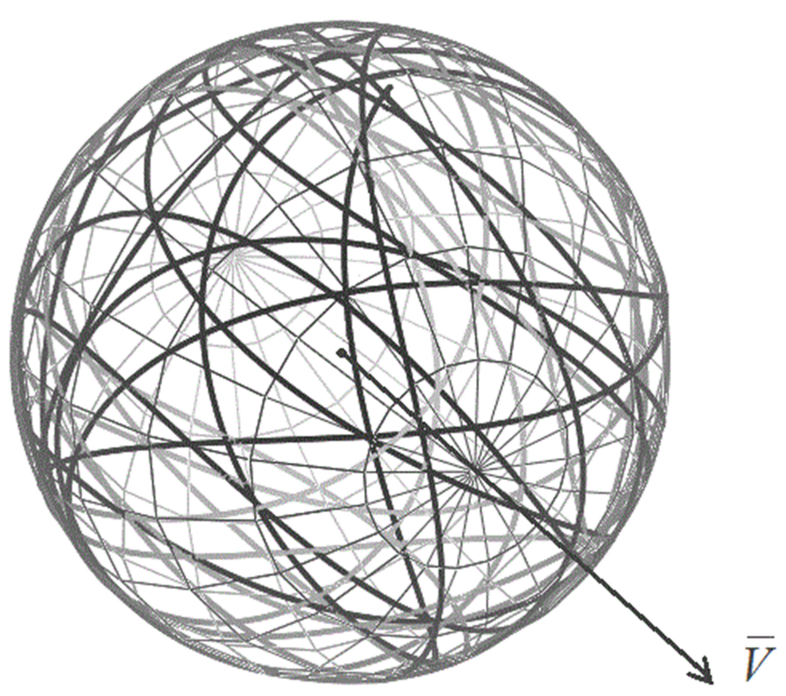
The fact that the ballistic coefficient remained constant throughout the entire time interval, despite a sharp increase in the ratio of the maximum aerodynamic torque to the maximum gravitational torque within time interval 2, indicates that the SamSat-218D was rotating uncontrollably. Therefore, we used the spatial model of the CubeSat angular motion and determined the angular velocity (2 deg/s) so that the ballistic coefficient simulated by this model coincided with the experimental one over the entire time interval. An illustration of the simulated spatial uncontrollable motion is shown as a hodograph (the motion of the SamSat-218D longitudinal axis represented on a sphere, Figure 13). The mean ballistic coefficient is 0.047 m2/kg with the standard deviation of 0.0005 m2/kg.
6. Conclusions
A method has been proposed to solve the inverse problem of estimating the ballistic coefficient of a CubeSat using the refined atmospheric density. The consideration of reference satellites sharing the same orbit or moving in close orbits enables an essentially accurate prediction of the motion mode of aerodynamically stabilized CubeSats and testing of their design concepts.
The method was verified using the long-term (2016–2022) SamSat-218D CubeSat position measurements. The ballistic coefficient depending on the descent altitude was reconstructed based on the design specifications of SamSat-218D (geometry, mass, moments of inertia, and static stability margin).
Since the end of 2020, we have seen that the aerodynamic torque significantly exceeds the gravitational torque; nevertheless, the ballistic coefficient remains constant. This fact indicates that the SamSat-218D motion mode relative to the center of mass is represented as uncontrolled spatial motion with the angular velocity of about two degree per second.
Using the proposed method to determine the motion mode of a CubeSat, we can refine its orbital lifetime.
Author Contributions
Conceptualization, I.B. and P.N.; methodology, I.B., I.T. and P.N.; software, I.T. and P.N.; validation, P.N.; formal analysis, I.T.; investigation, I.T. and P.N.; resources, P.N.; data curation, I.T. and P.N.; writing—original draft preparation, P.N.; writing—review and editing, I.B., I.T. and P.N.; visualization, P.N.; supervision, I.B.; project administration, I.B.; funding acquisition, I.B. All authors have read and agreed to the published version of the manuscript.
Funding
This research was supported by the state funding under grant number 0777-2020-0018. Grant recipients were selected from the competition involving research laboratories of higher educational institutions subordinate to the Ministry of Science and Higher Education of the Russian Federation.
Data Availability Statement
Not applicable.
Conflicts of Interest
The authors declare no conflict of interest.
Abbreviations
| TLE | Two-Line Element set; |
| SGP4 | Simplified Perturbations Model; |
| RK4 | classic Runge–Kutta method; |
| LEO | Low Earth Orbit. |
References
- Guo, J.; Pang, W.J.; Bo, B.; Meng, X.; Yu, X.; Zhou, J. Boom of the CubeSat: A statistic survey of Cubsats launch in 2003–2015. In Proceedings of the 67th International Astronautical Congress IAC-16-E2.4.5, Guadalajara, Mexico, 30 September 2016. [Google Scholar]
- Bryce Tech. Smallsats by the Numbers 2021. 2021. Available online: https://brycetech.com/reports/report-documents/Bryce_Smallsats_2021.pdf (accessed on 26 January 2022).
- Ariane 6. 2019. Available online: https://www.esa.int/Enabling_Support/Space_Transportation/Launch_vehicles/Ariane_6 (accessed on 26 January 2022).
- Rideshare Service for Light Satellites to Launch on Vega. 2020. Available online: https://www.esa.int/Enabling_Support/Space_Transportation/Rideshare_service_for_light_satellites_to_launch_on_Vega (accessed on 26 January 2022).
- JAXA Signs an Agreement with an Enterprise for Piggyback Launch Opportunities for Small Satellites. 2019. Available online: https://global.jaxa.jp/press/2019/12/20191204b.html (accessed on 26 January 2022).
- Mann, A. Rocket Lab: Private Spaceflight for Tiny Satellites. 2021. Available online: https://www.space.com/rocket-lab.html (accessed on 26 January 2022).
- Bouwmeester, J.; Guo, J. Survey of worldwide pico- and nanosatellite missions, distributions and subsystem technology. Acta Astronaut. 2010, 67, 854–862. [Google Scholar] [CrossRef]
- Swartwout, M. The First One Hundred CubeSats: A Statistical Look. J. Small Satell. 2013, 2, 213–233. Available online: https://jossonline.com/wp-content/uploads/2014/12/0202-The-First-One-Hundred-Cubesats.pdf (accessed on 26 January 2022).
- Swartwout, M. CubeSats and Mission Success: 2017 Update. In Proceedings of the 2016 Electronics Technology Workshop, Greenbelt, MD, USA, 26–29 June 2017; Saint Louis University: St. Louis, MO, USA, 2017. Available online: https://nepp.nasa.gov/workshops/etw2017/talks/28-JUN-WED/0900%20-%20swartwout%20etw%202017.pdf (accessed on 26 January 2022).
- Venturi, C.; Tolmasoff, M. Improving Mission Success of CubeSats; Aerospace Report; No. TOR-2017-01689; Aerospace Corporation: El Segundo, CA, USA, 2017; Available online: https://aerospace.org/sites/default/files/2018-07/TOR-2017-01689%20-%20Improving%20Mission%20Success%20of%20CubeSats.pdf (accessed on 26 January 2022).
- NORAD Two-Line Element Sets Current Data. Available online: https://celestrak.com/NORAD/elements/ (accessed on 26 January 2022).
- Kulu, E. Nanosats Database. Available online: https://www.nanosats.eu/ (accessed on 26 January 2022).
- Belokonov, I.V.; Timbai, I.A.; Barinova, E.V. Design Parameters Selection for CubeSat Nanosatellite with a Passive Stabilization System. Gyroscopy Navig. 2020, 11, 149–161. [Google Scholar] [CrossRef]
- Riano-Rios, C.; Sun, R.; Bevilacqua, R.; Dixon, W.E. Aerodynamic and gravity gradient based attitude control for CubeSats in the presence of environmental and spacecraft uncertainties. Acta Astronaut. 2021, 180, 439–450. [Google Scholar] [CrossRef]
- Schrello, D.M.; Davidson, P.H.; Juelich, O.C. Passive Aerodynamic Attitude Stabilization of Near-Earth Satellites, Volume I. Librations Due to Combined Aerodynamic and Gravitational Torques; WADD Technical Report 61-133; Aeronautical Systems Division, Air Force Systems Command, US Air Force, Wright-Patterson Air Force Base: Dayton, OH, USA, 1961. [Google Scholar]
- Belokonov, I.V.; Timbai, I.A.; Nikolaev, P.N. Analysis and Synthesis of Motion of Aerodynamically Stabilized Nanosatellites of the CubeSat Design. Gyroscopy Navig. 2018, 9, 287–300. [Google Scholar] [CrossRef]
- Belokonov, I.V.; Timbai, I.A.; Nikolaev, P.N. Approach for Estimation of Nanosatellite’s Motion Concerning of Mass Centre by Trajectory Measurements (IAA-B12-0703). In Proceedings of the 12th Symposium on Small Satellites for Earth Observation, Berlin, Germany, 6–10 May 2019; Sandau, R., Brieß, K., Gill, E., Eds.; IAA Book Series. International Academy of Astronautics: Paris, France, 2020; Volume 2, pp. 210–217. Available online: https://iaaspace.org/wp-content/uploads/iaa/Scientific%20Activity/conf/sseo2021/berlin2019proceedings.pdf (accessed on 26 January 2022).
- Vallado, D.A.; Finkleman, D. A critical assessment of satellite drag and atmospheric density modelling. Acta Astronaut. 2014, 95, 141–165. [Google Scholar] [CrossRef]
- Jacchia, L. Atmospheric Models in the Region from 110 to 2000 km. In CIRA 1972: COSPAR International Reference Atmosphere 1972; Akademie-Verlag: Berlin, Germany, 1972; pp. 227–338. [Google Scholar]
- Berger, C.; Biancale, R.; Barlier, F. Improvement of the empirical thermospheric model DTM: DTM-94—A comparative review of various temporal variations and prospects in space geodesy applications. J. Geod. 1998, 72, 161–178. [Google Scholar] [CrossRef]
- Bruinsma, S.; Thuillier, G.; Barlier, F. The DTM-2000 empirical thermosphere model with new data assimilation and constraints at lower boundary: Accuracy and properties. J. Atmos. Sol. Terr. Phys. 2003, 65, 1053–1070. [Google Scholar] [CrossRef]
- Hedin, A.E. MSIS-86 thermospheric model. J. Geophys. Res. 1987, 92, 4649–4662. [Google Scholar] [CrossRef]
- Hedin, A. Extension of the MSIS thermospheric model into the middle and lower atmosphere. J. Geophys. Res. 1991, 96, 1159–1172. [Google Scholar] [CrossRef]
- Picone, J.; Hedin, A.; Drob, D.; Aikin, A. NRLMSISE-00 empirical model of the atmosphere: Statistical comparisons and scientific issues. J. Geophys. Res. 2002, 107, SIA 15-1–SIA 15-16. [Google Scholar] [CrossRef]
- Marcos, F.A.; Bowman, B.R.; Sheehan, R.E. Accuracy of Earth’s thermospheric neutral density models. In Proceedings of the AIAA/AAS Astrodynamics Specialist Conference, Keystone, CO, USA, 21–26 August 2006. [Google Scholar] [CrossRef]
- Krebs Gunter, D. “Pion”. Gunter’s Space Page. Available online: https://space.skyrocket.de/doc_sdat/pion.htm (accessed on 26 January 2022).
- Nicholas, A.C.; Gilbreath, G.C.; Thonnard, S.E.; Kessel, R.A.; Lucke, R.; Sillman, C.P. The Atmospheric Neutral Density Experiment (ANDE) and Modulating Retroreflector in Space (MODRAS): Combined flight experiments for the space test program. In Proceedings of the Optics in Atmospheric Propagation and Adaptive Systems V, Crete, Greece, 20 March 2003; Volume 4884. [Google Scholar] [CrossRef]
- Pilinski, M.D.; Palo, S.E. An Innovative Method for Measuring Drag on Small Satellites. In Proceedings of the 23th Annual AAIA/USU Conference on Small Satellite, Logan, UT, USA, 10–13 August 2009; Available online: https://digitalcommons.usu.edu/cgi/viewcontent.cgi?article=1311&context=smallsat (accessed on 26 January 2022).
- Pilinski, M.D. Analysis of a Novel Approach for Determining Atmospheric Density from Satellite Drag. Master’s Thesis, University of Colorado, Boulder, CO, USA, 2008. [Google Scholar]
- Nicholas, A.; Finne, T.; Galysh, J. SpinSat mission overview. In Proceedings of the 27th Annual AAIA/USU Conference on Small Satellite, Logan, UT, USA, 19–22 September 2013. [Google Scholar]
- Zhao, Z.; Wang, Z.; Zhang, Y. A Spherical Micro Satellite Design and Detection Method for Upper Atmospheric Density Estimation. Int. J. Aerosp. Eng. 2019, 2019, 1758956. [Google Scholar] [CrossRef]
- Thoemel, J.; Singarayar, F.; Scholz, T.; Masutti, D. Status of the QB50 cubesat constellation mission. In Proceedings of the 65th International Astronautical Congress, Toronto, ON, Canada, 21 January 2014. [Google Scholar]
- Belokonov, I.V.; Ivanov, D.S.; Ovchinnikov, M.Y.; Pen’kov, V.I. Passive System for the Angular Damping of the SAMSAT-QB50 Nanosattelite. J. Comput. Syst. Sci. Int. 2019, 58, 774–785. [Google Scholar] [CrossRef]
- Nier, A.O.; Potter, W.E.; Hickman, D.R.; Mauersberger, K. The open-source neutral-mass spectrometer on Atmosphere Explorer-C, -D, and -E. Radio Sci. 1973, 8, 271–276. [Google Scholar] [CrossRef]
- Hoffman, J.H.; Hanson, W.B.; Lippincott, C.R.; Ferguson, E.E. The magnetic ion-mass spectrometer on Atmosphere Explorer. Radio Sci. 1973, 8, 315–322. [Google Scholar] [CrossRef]
- Niemann, H.B. An atomic oxygen beam system for the investigation of mass spectrometer response in the upper atmosphere. Rev. Sci. Instrum. 1972, 43, 1151–1161. [Google Scholar] [CrossRef]
- Emmert, J.T. Thermospheric mass density: A review. Adv. Space Res. 2015, 56, 773–824. [Google Scholar] [CrossRef]
- Champion, K.S.W.; Marcos, F.A. The triaxial-accelerometer system on atmosphere explorer. Radio Sci. 1973, 8, 297–303. [Google Scholar] [CrossRef]
- Doornbos, E. Thermospheric Density and Wind Determination from Satellite Dynamics. Ph.D. Dissertation, University of Delft, Delft, The Netherlands, 2011. [Google Scholar]
- Vallado, D.A.; Crawford, P. SGP4 orbit determination. In Proceedings of the AIAA/AAS Astrodynamics Specialist Conference and Exhibit, Honolulu, HI, USA, 18–21 August 2008. [Google Scholar] [CrossRef]
- Shi, C.; Li, W.; Li, M.; Zhao, Q.; Sang, J. Calibrating the scale of the NRLMSISE00 model during solar maximum using the two line elements dataset. Adv. Space Res. 2015, 56, 1–9. [Google Scholar] [CrossRef]
- Krzysztof, S. Impact of the atmospheric drag on Starlette, Stella, Ajisai, and Lares Orbits. Artif. Satell. 2015, 50, 1–18. [Google Scholar] [CrossRef]
- Doornbos, E.; Klinkrad, H.; Visser, P. Use of two-line element data for thermosphere neutral density model calibration. Adv. Space Res. 2008, 41, 1115–1122. [Google Scholar] [CrossRef]
- Li, B.; Zhang, Y.; Huang, J.; Sang, J. Improved orbit predictions using two-line elements through error pattern mining and transferring. Acta Astronaut. 2021, 188, 405–415. [Google Scholar] [CrossRef]
- Lu, Z.; Hu, W. Estimation of ballistic coefficients of space debris using the ratios between different objects. Chin. J. Aeronaut. 2017, 30, 1204–1216. [Google Scholar] [CrossRef]
- Belokonov, I.V.; Timbai, I.A.; Nikolaev, P.N.; Orazbaeva, U.M. Analysis of SamSat-218D nanosatelite motion acording to trajectory measurements, Vestnik of Samara University. Aerosp. Mech. Eng. 2019, 18, 18–28. [Google Scholar] [CrossRef]
- Belokonov, I.V.; Timbai, I.A.; Nikolaev, P.N. Reconstruction of motion relative to the center of mass of a low-altitude nanosatellite from trajectory measurements. In Proceedings of the IAC 2021 Congress Proceedings, 72nd International Astronautical Congress (IAC), Dubai, United Arab Emirates, 25–29 October 2021. IAC-21-B4.3.8. [Google Scholar]
- Hoots, F.R.; Roehrich, R.L. Models for Propagation of NORAD Element Sets. Spacetrack Report NO. 3. 1980. Available online: http://www.celestrak.com/NORAD/documentation/spacetrk.pdf (accessed on 26 January 2022).
- Press, W.H. Numerical Recipes: The Art of Scientific Computing, 3rd ed.; Cambridge University Press: New York, NY, USA, 2007. [Google Scholar]
- Wahba, G. Spline Models for Observational Data. In CBMS-NSF Regional Conference Series in Applied Mathematics; University City Science Center: Philadelphia, PA, USA, 1990. [Google Scholar] [CrossRef]
- Belokonov, I.V.; Kramlikh, A.V.; Timbai, I.A. Low-orbital transformable nanosatellite: Research of the dynamics and possibilities of navigational and communication problems solving for passive aerodynamic stabilization. J. Adv. Astronaut. Sci. 2015, 153, 383–397, IAA-AAS-DyCoSS2-14-04-10. [Google Scholar]
- Barinova, E.V.; Belokonov, I.V.; Timbai, I.A. Preventing Resonant Motion Modes for Low-Altitude CubeSat Nanosatellites. Gyroscopy Navig. 2022, 12, 350–362. [Google Scholar] [CrossRef]
- Kirillin, A.; Belokonov, I.; Timbai, I.; Kramlikh, A.; Melnik, M.; Ustiugov, E.; Egorov, A.; Shafran, S. SSAU nanosatellite project for the navigation and control technologies demonstration. J. Procedia Eng. 2015, 104, 97–106. [Google Scholar] [CrossRef]
- Abrashkin, V.I.; Voronov, K.E.; Dorofeev, A.S.; Piyakov, A.V.; Puzin, Y.Y.; Sazonov, V.V.; Semkin, N.D.; Filippov, A.S.; Chebukov, S.Y. Detection of the Rotational Motion of the AIST-2D Small Spacecraft by Magnetic Measurements. Cosmic Res. 2019, 57, 48–60. [Google Scholar] [CrossRef]
- Sadovnichii, V.A.; Panasyuk, M.I.; Amelyushkin, A.M.; Bogomolov, V.V.; Benghin, V.V.; Garipov, G.K.; Kalegaev, V.V.; Klimov, P.A.; Khrenov, B.A.; Petrov, V.L. “Lomonosov” Satellite—Space Observatory to Study Extreme Phenomena in Space. Space Sci. Rev. 2017, 212, 1705–1738. [Google Scholar] [CrossRef]
- Fifth Anniversary of the First Launch from Vostochny. 2021. Available online: http://en.roscosmos.ru/22086/ (accessed on 26 January 2022).
- Soyuz 2-1v Launch Vehicle. Available online: https://spaceflight101.com/spacerockets/soyuz-2-1v (accessed on 26 January 2022).
- Progress Rocket Space Centre. Available online: https://www.samspace.ru (accessed on 26 January 2022).
- Innoter Geospatial Agency. AIST-2D. Available online: https://innoter.com/en/satellites/aist-2d/ (accessed on 26 January 2022).
- Wua, S.; Chen, W.; Cao, C.; Zhang, C.; Mu, Z. A multiple-CubeSat constellation for integrated earth observation and marine/air traffic monitoring. Adv. Space Res. 2021, 67, 3712–3724. [Google Scholar] [CrossRef]
Figure 1.
(a) Phase portrait (|a| ≥ 2c), here lines 1 are phase trajectories of rotation motion mode, line 2 is phase trajectory of oscillatory motion mode and line 3 is separatrix; (b) phase portrait (c > 0.5|a|), here lines 1 are phase trajectories of rotation motion mode, line 2 is phase trajectory of oscillatory motion mode relative to the equilibrium position α, lines 3 are phase trajectories of oscillatory motion mode relative to the equilibrium position α*, lines 4 and 5 are separatrices.

Figure 2.
Procedures for identification of CubeSat motion mode relative to the mass center.

Figure 3.
Payload fairing with Lomonosov, AIST-2D, and SamSat-218D satellites installed [58].
Figure 3.
Payload fairing with Lomonosov, AIST-2D, and SamSat-218D satellites installed [58].

Figure 4.
The laboratory photo of SamSat-218D.

Figure 5.
Changes in the satellite altitudes calculated using TLE files: MVL-300, AIST-2D, and SamSat-218D.
Figure 5.
Changes in the satellite altitudes calculated using TLE files: MVL-300, AIST-2D, and SamSat-218D.

Figure 6.
Estimated ballistic coefficients of (a) MVL-300, (b) AIST-2D, and (c) SamSat-218D.

Figure 7.
The corrected ballistic coefficient of SamSat-218D (Step 4).

Figure 8.
Changes in the altitudes of the satellites calculated using TLE files: MVL-300, AIST-2D, Tianwang-1A, SamSat-218D, Tianwang-1B, and Tianwang-1C.
Figure 8.
Changes in the altitudes of the satellites calculated using TLE files: MVL-300, AIST-2D, Tianwang-1A, SamSat-218D, Tianwang-1B, and Tianwang-1C.

Figure 9.
The slope coefficient of the ballistic coefficient data dependency on the mean drag coefficient within the measurement period.
Figure 9.
The slope coefficient of the ballistic coefficient data dependency on the mean drag coefficient within the measurement period.

Figure 10.
The corrected ballistic coefficient of SamSat-218D (Step 5).

Figure 11.
The ratio of the maximum aerodynamic torque to maximum gravitational torque.

Figure 12.
(a) The simulated angle of attack and (b) the simulated time-dependent ballistic coefficient (angular velocity is 0.1 deg/s).
Figure 12.
(a) The simulated angle of attack and (b) the simulated time-dependent ballistic coefficient (angular velocity is 0.1 deg/s).

Figure 13.
Hodograph of the CubeSat longitudinal axis relative to the trajectory coordinate system on a single sphere for the initial angular velocity of 2 deg/s.
Figure 13.
Hodograph of the CubeSat longitudinal axis relative to the trajectory coordinate system on a single sphere for the initial angular velocity of 2 deg/s.


Table 1.
Classification of regions for the influence of environmental torques.
| Regions of Influence | Altitude Range | Environmental Effects |
|---|---|---|
| Region I | Below 300 km | Aerodynamic torques dominate angular motions |
| Region II | From 300 to 650 km | Aerodynamic and gravitational torques are comparable |
| Region III | From 650 to 1000 km | Aerodynamic, gravitational, and solar torques are comparable |
| Region IV | Above 1000 km | Solar and gravitational torques dominate angular motions |
Table 2.
Comparison of 3U CubeSat SamSat-218D and microsatellite AIST 2D.
| Feature | SamSat-218D (3U CubeSat) | AIST 2D (Micro Satellite) |
|---|---|---|
| Maximum angular acceleration at 480 km altitude caused by aerodynamic torque, (s−2) | 1.8 × 10⁻⁶ | ~10−8 |
| Averaged ballistic coefficient, (m2/kg) | 0.048 | 0.0227 |
| Ratio of the maximum value of ballistic coefficient to the minimum one | 4.75 | ~1.73 |
Table 3.
Main parameters of Lomonosov.
| Parameter | Value |
|---|---|
| NORAD ID | 41,464 |
| Mass, kg | 625 |
| ADCS | triaxial |
Table 4.
Main parameters of AIST-2D.
| Parameter | Value |
|---|---|
| NORAD ID | 41,465 |
| Mass, kg | 531 |
| ADCS | Triaxial |
| B, m2/kg | 0.0227 |
Table 5.
Main parameters of SamSat-218D.
| Parameter | Value |
|---|---|
| NORAD ID | 41,466 |
| Deployment angle, deg (initial angle of attack in orbital plane) | 80 (in orbital plane) |
| Deployment angular velocity, deg/s | Unspecified |
| Mass, kg | 1.82 |
| Main inertia moments, kg·m2 | 0.00402; 0.01422; 0.01454 |
| Static stability margin, m | 0.06 |
Disclaimer/Publisher’s Note: The statements, opinions and data contained in all publications are solely those of the individual author(s) and contributor(s) and not of MDPI and/or the editor(s). MDPI and/or the editor(s) disclaim responsibility for any injury to people or property resulting from any ideas, methods, instructions or products referred to in the content. |
© 2023 by the authors. Licensee MDPI, Basel, Switzerland. This article is an open access article distributed under the terms and conditions of the Creative Commons Attribution (CC BY) license (https://creativecommons.org/licenses/by/4.0/).
Share and Cite
MDPI and ACS Style
Belokonov, I.; Timbai, I.; Nikolaev, P. Studies of Satellite Position Measurements of LEO CubeSat to Identify the Motion Mode Relative to Its Center of Mass. Aerospace 2023, 10, 378. https://doi.org/10.3390/aerospace10040378
AMA Style
Belokonov I, Timbai I, Nikolaev P. Studies of Satellite Position Measurements of LEO CubeSat to Identify the Motion Mode Relative to Its Center of Mass. Aerospace. 2023; 10(4):378. https://doi.org/10.3390/aerospace10040378
Chicago/Turabian StyleBelokonov, Igor, Ivan Timbai, and Petr Nikolaev. 2023. "Studies of Satellite Position Measurements of LEO CubeSat to Identify the Motion Mode Relative to Its Center of Mass" Aerospace 10, no. 4: 378. https://doi.org/10.3390/aerospace10040378
Note that from the first issue of 2016, this journal uses article numbers instead of page numbers. See further details here.