
Towards Accurate Vortex Separation Simulations with RANS Using Improved k-kL Turbulence Model

1
Defense Industries Research and Development Institute (TÜBİTAK SAGE), Gökçeyurt mah., Mamak, Ankara 06270, Türkiye
2
Mechanical Engineering Department, Middle East Technical University, Üniversiteler mah. Dumlupınar Blv. No: 1, Çankaya, Ankara 06800, Türkiye
*
Author to whom correspondence should be addressed.
Aerospace 2023, 10(4), 377; https://doi.org/10.3390/aerospace10040377
Submission received: 7 December 2022
/
Revised: 9 January 2023
/
Accepted: 12 January 2023
/
Published: 18 April 2023
Abstract
:In this study, we present our improved RANS results of the missile aerodynamic flow computation involving leading edge vortex separation. We have used our in-house tailored version of the open source finite volume solver FlowPsi. An ongoing study in the NATO STO Applied Vehicle Technologies Panel (AVT-316) has revealed that a highly maneuverable missile configuration (LK6E2) shows unusual rolling moment characteristics due to the vortex–surface interactions occurring during wing leading edge separation of vortices. We show the performance of the recently developed k- turbulence model for this test problem. This turbulence model is shown to have superior capabilities compared to other widely used turbulence models, such as Spalart–Allmaras and shear stress transport. With the k- turbulence model, it is possible to achieve more realistic computational results that agree better with the physical data. In addition, we propose improvements to this turbulence model to achieve even better predictions of rolling moment behavior. Modifications based on turbulence production terms in the k- turbulence model significantly improved the predicted rolling moment coefficient, in terms of accuracy and uncertainty.
1. Introduction
Computational fluid dynamics (CFD) is a widespread practice for predicting the flow field around military air vehicles. Nowadays, CFD applications are not limited to the analysis of certain flow conditions; hence, CFD has become a standard design tool with the advancing computer technologies. One of the few exceptions is the applications sensitive to separation and vortex features. Standard, relatively low-cost CFD tools have not been proven to perform adequately for the separated flows with vortex features [1,2,3]. More challenges are experienced when vortex interactions with other flow features, such as shock waves in transonic and supersonic speeds, are considered [4]. Likewise, the interactions between multiple vortices, incorporated in most high angle of attack flows, are challenging to resolve with standard CFD techniques [5].
The NATO Science and Technology Organization (STO) Applied Vehicle Technology (AVT) panel established a Task Group identified as AVT-316 (Vortex Interaction Effects Relevant to Military Air Vehicle Performance). A branch of the group was devoted to the assessment of the current capabilities of CFD to predict missile aerodynamic characteristics for flows containing multiple vortex interactions. LK6E2 was one of the research test cases developed to investigate vortex interactions on highly maneuverable transonic missiles. The initial collaborative analysis of the test case was published during special sessions at AIAA 2022 SciTech Conference [6,7]. It was shown that the flow solver and the turbulence model greatly impact the prediction of the flow field and aerodynamic coefficients of these missiles at high flow angles and transonic speeds. Notably, the variation in the rolling moment coefficient resulting from different computations was huge, which would potentially cause misleading stability and control assessments during the design and analysis of similar transonic missile airframes.
During the NATO STO AVT-316 work, to which the authors of the current paper have contributed, it was observed that nearly all statistical turbulence models fail to make accurate predictions of the flow field around an LK6E2 missile in certain flow conditions [6,8]. Higher order turbulence models, where the elements of Reynolds stress tensor are computed, e.g., (algebraic) RSM methods, provide more realistic predictions. However, these turbulence models are more difficult to apply and require significantly more computational resources. Apart from those, hybrid RANS-LES methods consume even more computational sources. Hence these methods are still considered impractical for simulation sets of multiple flow conditions, though they have been shown to compute better results [7,8]. For these reasons, the current study put effort into achieving improved RANS results within the bounds of the statistical turbulence models, which are considered more productive in practice.
In the CFD simulations of industrial-scale airframes, turbulence physics still has to be modeled by RANS or hybrid RANS-LES methods, due to the limitations of today’s computing capabilities. The hybrid RANS-LES approach can only be utilized for much fewer conditions, compared to the whole range of flight conditions. Therefore, RANS modeling is considered the standard practice, and it will remain in its position in the near future. For this reason, investigations in this study are limited to RANS-based computations. Within the RANS context, our group explored a turbulence model that will perform better in vortical flow simulations. We have found an old, but understudied, model by Rotta, which was rediscovered by Menter et al. [9,10] and improved by Abdol-Hamid [11,12] in recent years. The k- model is based on the turbulence length scale, and Menter claims that the model has LES-like qualities in separating flow simulations. This characteristic may solve the inadequacies of common RANS methods in separated flows.
Vortex capturing capabilities of our in-house flow solver have recently been improved by the implementation of the k- turbulence model [13,14]. The new implementation has been verified using the results of model developers [11]. The first results have been obtained on the fin trailing vortex case, which was experimentally studied by Beresh et al. [15,16,17]. This test case is worthwhile for assessing the vortex simulation capabilities of the turbulence models, since the test data involve detailed particle image velocimetry measurements of a fin-tip vortex for several downstream stations. Therefore, the decay of the vortex core can be observed in detail. It was shown that flow variables within the vortex core are more accurately predicted. The vortex is better preserved along the downstream path using the k- turbulence model, compared to other equation models based on the Boussinesq hypothesis [14].
These promising results motivated us to employ the k- turbulence model in the NATO STO AVT-316 study. Significant improvements in the LK6E2 test case results are observed over the standard models. A parallel study with several correction methods on the k--SST model was also conducted. The latter study also the improved k--based solutions. Therefore, the turbulence production term-based varieties and compressibility correction methods are implemented on the standard k- model to further improve the model.
In the current study, we have two objectives. Our primary objective is to assess the performance of the k- turbulence model on the prediction of vortex separation occurring on the wings of the selected transonic missile case. The other objective is to improve the k- turbulence model capabilities on the same problems using the experience on the improvements on other turbulence models. This paper presents the results of LK6E2 test case computations conducted with our in-house flow solver. The benchmark results between k- and k--SST turbulence models are also presented to show the achievements with the k- turbulence model, including the improved versions developed within the current study. Comparisons are made against available experimental aerodynamic coefficient data where applicable. Our improvements resulted in significantly better results in flows with vortices.
The research questions arise from the NATO STO AVT-316 study, which is further validated by the study of the authors:
- The effect of the vortices on the aircraft body is often insignificant on aircraft aerodynamics, due to the location and sizing. Most turbulence models are not calibrated for such configurations. However, these contributions are important for missiles with multiple lifting surfaces on high-incidence angle conditions. What is the prominent turbulence model to be employed for these problems?
- The underlying problem for the inaccuracies of classical turbulence models at vortical flows is the excessive turbulence production, as shown in Ref. [14]. Is this problem the source of inaccuracies in the roll moment of the simulations in the NATO STO AVT-316 group?
- What is the state-of-the-art turbulence model for accurate vortex predictions? Can we provide a remedy to excessive turbulence production on this model and further improve these predictions?
2. LK6E2 Test Case and the Problem Description
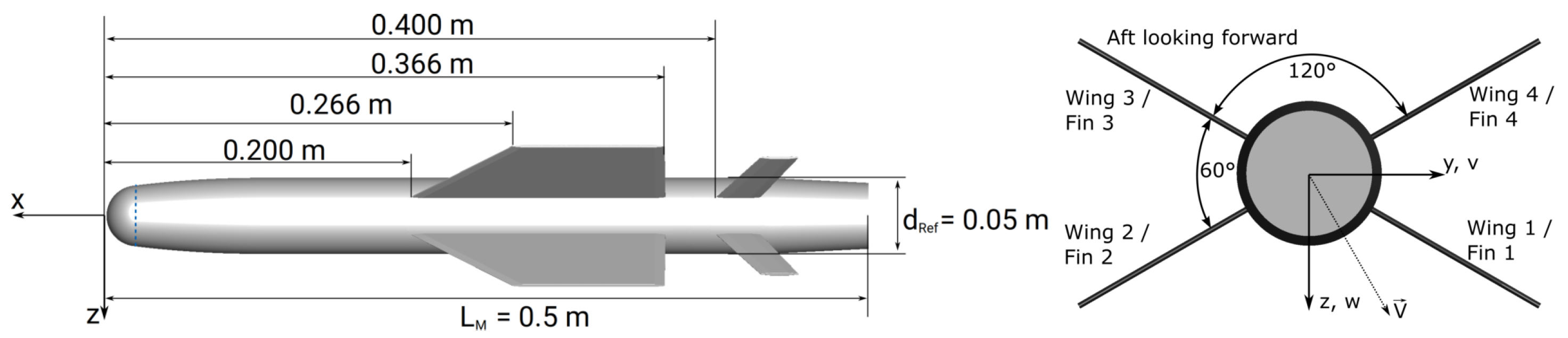
The LK6E2 model was developed by the German Aerospace Center (DLR) to investigate wing vortex interactions. The test model has a body starting with a blunt nose and ending with a boattail at the rear. The model has a considerably large wing set and a second fin set at the rear with a small wetted area. As seen in Figure 1, LK6E2 is a representative model for a transonic missile concept designed for the bank-to-turn control method [6] with large wing-like fins in the middle section. To improve the lifting surface area, the angle between sideward wings/fins is 60°, while this angle between upper/lower wings/fins is 120°. As the model is intended to undergo a wind tunnel testing activity, it is defined as a scaled model (1:3), with body diameters and lengths of 5 and 50 cm, respectively. Other geometric details are given in Figure 1. The coordinate frame is fixed to the body. The X, Y, and Z axes point to the nose-tip, starboard side, and downward, respectively.
In external aerodynamic flows, it is a common practice to define the flow conditions through the free stream Mach number, thermostatic conditions (pressure and temperature), and flow direction. Although there are several ways to define the free stream flow direction, the pitch-roll (-) arrangement was adopted for the LK6E2 test case. The velocity components of the missile expressed in the body coordinate frame are denoted as u, v, and w, which make up the velocity vector, with respect to the flow. The relation between pitch-roll (or incidence-roll) angles and velocity components is given in Equation (1).
As a result of the high maneuvrability requirements of the LK6E2 missile concept, the airframe needs to be exposed to flow conditions with a high angle of incidence during critical stages of the flight. The high incidence angle leads to inevitable local separations on the flow field surrounding the missile surface, which results in non-linearities in the aerodynamic coefficients with changing inflow conditions. An illustration of these characteristics was experienced during LK6E2 wind tunnel tests in the transonic wind tunnel of Göttingen (TWG) and the high-speed wind tunnel (HST) in Amsterdam. The test results obtained from both wind tunnel agree that the rolling moment coefficient shows a non-linear behavior at 45-degree roll orientation and incidence angles between 15 and 20 degrees [6]. The flow condition range where this non-linearity is observed was determined as the test condition for LK6E2, as some challenges in the numerical simulations arose. The flow condition range of interest is summarized in Table 1.
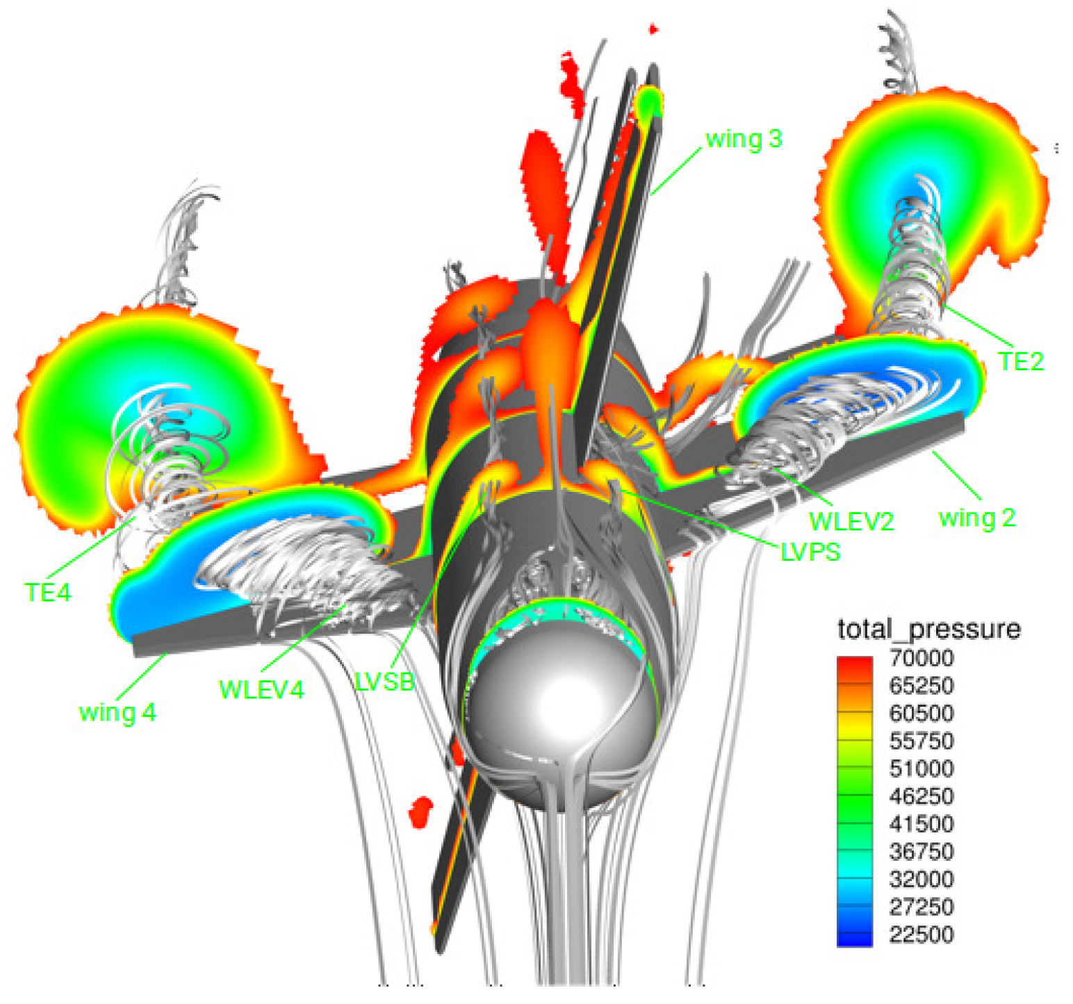
The flow over LK6E2 geometry involves the interactions of multiple vortices at these conditions. The initial computations with the freestream conditions given in Table 1 resulted in the flow topology shown in Figure 2 [6]. Wing leading edge vortices are pronounced for Wing 2 and Wing 4 (WLEV2 and WLEV4). These vortices are effective throughout their respective wing surfaces. Therefore, the pressure distribution on these wings and, consequently, the rolling moment are very sensitive to vortex predictions, as will be shown later in this paper.
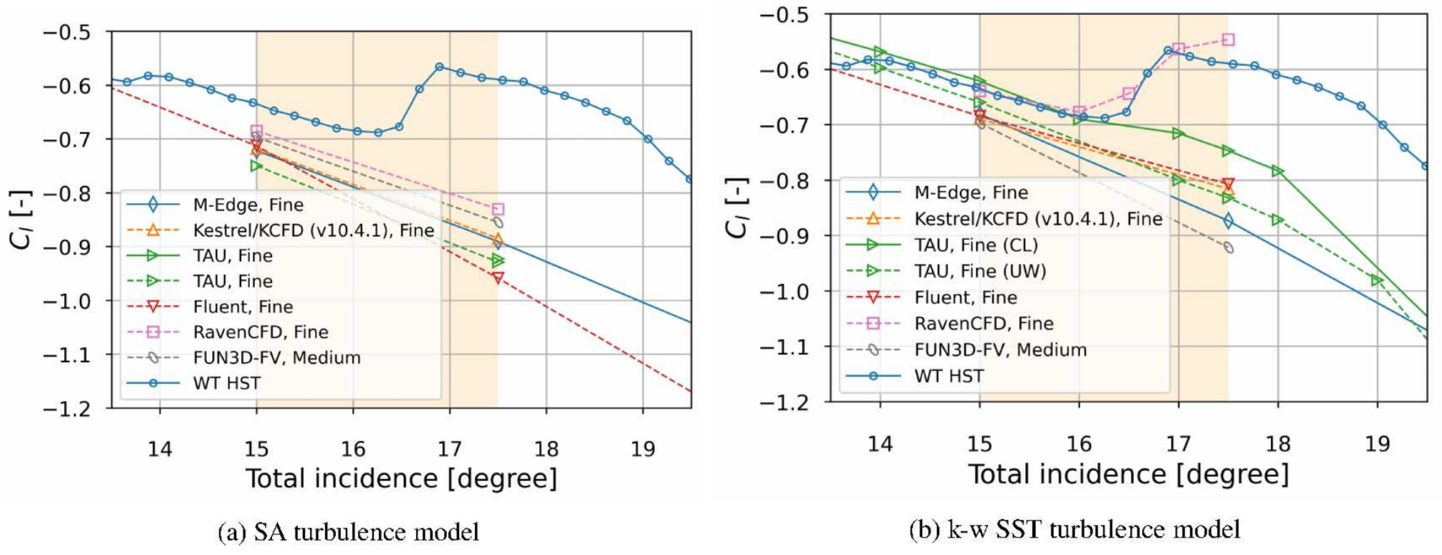
The NATO STO AVT-316 study shows that current turbulence models especially fall short of predicting the rolling moment at the angle of attack zone shaded in Figure 3. The only SST-based result agreeing with the experimental data is evaluated as an outlier, since all other solutions, including ours with the SST model, show similar behavior. Indeed, no clear reason for this difference could be found by the NATO STO AVT team [6]. The AVT-316 team reported strong vortex–vortex and vortex–body interactions at this zone. This behavior is shown to be independent of mesh resolution. Although the missile geometry and flow conditions are generated and ’tailored’ for this study, the reported issue is not a fabricated problem. We have seen similar discrepancies between the wind tunnel data and CFD results in our missile development programs. Therefore, the STO AVT-316 study leads our team to a captivating problem of turbulence models capable of capturing vortex mechanisms. The model should be capable of predicting the sudden drop in the roll moment around 17 degrees incidence angle, hence the complex vortex–surface interactions at this zone.
3. Flow Solver
The flow solver utilized in this study is a tailored version of the open source code FlowPsi, which is a compressible RANS solver based on the finite volume method [18]. Extensive information on the theory and methods behind the code is provided in the user manual available with the source distribution [19]. The solver uses a second-order Crank–Nicholson time-stepping for time integration. Inviscid fluxes are discretized with a second-order HLLC scheme, an upwind method developed by Toro et al. [20]. A low dissipation kinetic energy consistent flux discretization is also available. Inviscid flux extrapolation is limited by Venkatakrishnan [21,22] or Barth–Jespersen [23] limiters, alternatively. The code accepts unstructured meshes with various types of element topology co-existing, as it has a cell-centered formulation. The SST-2003 [24] is one of the turbulence models that has been utilized in the current study. The k--MEAH2015 [12] model is implemented by the authors of this article.
Our solver already had a number of turbulence models. We initially tested the Spalart–Allmaras and k- models in the early phases of the NATO-AVT study. Considering the large computational mesh sizes, we have eliminated the Spalart–Allmaras model and narrowed our presented results to k- SST. Note that our SA and SST results are in line with other AVT participants. Therefore, our solver and turbulence model implementations are verified. Our results of the SA and SST turbulence models with the results of other AVT study are reported, and our solver is shown to agree with other studies [6].
4. An Improved Vortex Separation Capable - Turbulence Model
As reported in Section 2 and Figure 3, both the Spalart–Allmaras and Shear Stress Transport turbulence models fail to predict vortex interactions at moderate to high flight angles. The members of the AVT-316 group consistently made the same observation, apart from one outlier. We have proposed a few methods to improve the prediction performance. Then, we combined these to achieve better results. The first method is the application of well-known rotational corrections. Applying these corrections improved the -ω-based results at the mentioned flow range, but the improvement did not resolve the problem, as will be shown in Section 6.4.
We have experimented with the idea of using a more vortex-capable turbulence model. One notable candidate is Rotta’s -based model [25]. Menter and Egorov implemented a new turbulence model based on Rotta’s original idea [9] and claimed that the new model has LES-like properties [10,26]. This feature is promising for the vortical flows, since the separated flows are often simulated better with LES-based methods. The k-kL method is developed and reported by Abdol-Hamid, and compressible extensions are provided [11,12]. Therefore, we have implemented and tested Abdol-Hamid’s method on a compressible separated flow around a missile fin [14].
4.1. Verification of the Implementation
The k-kL-MEAH2015 turbulence model formulation, development procedure, and extensive reference data for the validation cases were provided by Abdol-Hamid et al. [11,12,27]. The model formulation is available on the NASA Turbulence Modeling Resource website, which forms a valuable collection and classification of standard turbulence models [28]. The authors of the article followed the available documentation, while implementing the model into their solver. The formulation of the implemented model is given in (2) and (3). The turbulence quantities influence the flow variables via the turbulent viscosity parameter, computed as .
The production term of the turbulence transport equations is calculated by (4). The major component of turbulence production is the term containing the local shear strain appearing in the standard version. According to this formulation, the major component of the turbulence source is , given that .
We have followed the verification steps in the original studies of Abdol-Hamid. The implementation was verified with the standard test case simulations for which the computational data are available [28]. Verification with the 2D flat plate and 2D bump cases was reported previously by the authors [14]. Verification data is composed of pressure and skin friction distributions throughout the wall surface and the velocity and turbulent parameter (k, ) profiles within the boundary layer extracted at a couple of sections. The published verification cases were run using the CFL3D and FUN3D codes, maintained by NASA, and the TAU code, maintained by the German Aerospace Center (DLR). All flow field parameters were very close to those calculated by the other three codes. An extensive discussion regarding the verification of our implementation of the k--MEAH2015 model is given in the study of Dikbaş and Baran [14].
The results of the k- model for standard turbulence test cases are in-line with other standard models, showing that the k- model is a reliable turbulence model. In order to reveal the scale-adaptive characteristics of the model claimed by Menter et al. and also to evaluate the model’s performance in vortical flows, the implemented model was further validated with a simplified vortical flow case. The reference experimental study conducted by Beresh et al. [15,16,17] investigates the dynamics of a single vortex that is separated from an isolated fin exposed to an external flow. The authors of the current paper showed that the k- turbulence model predicts more realistic turbulent characteristics within the vortex core, compared to other equation models. Therefore, better agreement with the experimentally determined flow field could be obtained. These validation results can also be seen in Ref. [14]. The results show that the vortex core originating from the fin is preserved much better with the k- method than with the standard models. The study claims that the k- model prevents excessive turbulence production at the vortex core, unlike the SA and SST models.
4.2. Overview of Improvements on the k- Model
As the second step in our search for a better vortex-capable turbulence model, we have implemented the k- turbulence model, a relatively new method tested for the current type of problem for the first time. As it will be shown in Section 6, the results were surprisingly good, yet there is room for improvement. To achieve more accurate predictions for the transonic flow problems involving strong vortex interactions, we have put effort into the optimization of the k- turbulence model.
Several sources of error in the flowfield calculations involving vortical compressible flows are as follows:
- A shear layer is formed between the vortex and the freestream flow, and the interaction effects with shock waves and surfaces should be considered carefully [32].
We are addressing these three problems in our research program. The third problem is determined as the main focus of this paper; therefore, improvements of the k- turbulence model are sought with the aim of enhanced RANS simulations for the described test problem. With the application of different turbulence production formulations and compressibility and free jet corrections, more realistic predictions could be made, as presented in Section 6.
For this purpose, we have implemented the k- model to allow modifications to the turbulence production term. The new implementation permits choosing alternative production formulations. These production formulation alternatives may make use of either local strain magnitude (S), local vorticity magnitude (), or both S and . The original implementation of Abdol-Hamid [11] is based on total strain tensor magnitude. We have adopted different production formulations based on the reference works done for other turbulence models for the turbulence model. The designations associated with each option are recommended considering the principles endorsed in NASA Turbulence Modeling Resource [28]. In this study, we have replaced the major component of the production term with Kato’s [33] formulation. Therefore, the major total strain term, , in the original model is replaced by . Likewise, another alternative that uses only vorticity magnitude can be generated, i.e., . We expect that the employment of the vorticity magnitude in the calculation of turbulence production helps avoid the unphysical accumulation of computed turbulent quantities caused by shear stress.
The k-kL model implemented in our solver also supports the vorticity corrections [34,35] widely used for a broad range of rotational flows. Among these, we have adopted the rotation/curvature (RC) correction, which is the one customized by Menter et al. [36] for the two-equation SST model. We have also refined the RC correction for our k-kL turbulence model implementation. It has already been shown that the vorticity corrections are able to provide better vortex predictions via compensation of the over-dissipative character of Boussinesq hypothesis-based turbulence models [31,37]. The present test case, however, will give the opportunity for the performance evaluation of the RC correction in the context of the prediction of the formation of a leading edge vortex. Table 2 summarizes the alternative turbulence production and vorticity correction formulations.
Another improvement to the k- model in our implementation is the support for different types of compressibility corrections. In our solver, the compressibility correction is accompanied by free shear correction, as suggested by Abdol-Hamid [12] in their jet correction definition for the k--MEAH2015+J turbulence model. The formulation of the compressibility correction in the current implementation is generalized with modifiable coefficients. As given in Equation (5), the coefficients of destruction terms in k and equations are increased by factors depending on the compressibility correction parameter, . This parameter is given in Equation (6) as a function of the turbulent Mach number, . In order to eliminate low subsonic speeds from the compressibility correction, a cut-off value for , denoted as may be used as suggested by Wilcox [38]. The original formulation of Sarkar et al. [39] does not contain such a threshold. The free shear correction is active unless the compressibility correction is turned off. Table 3 summarizes some alternatives that can be applied with the improved k- model. The modified Wilcox correction represents the alternative, described by Abdol-Hamid et al. [12], as k--MEAH2015+J.
It should be noted that the alternative production formulations actively change the turbulence model only at high-curvature or high-vorticity flows. These formulations do not alter the results for standard turbulence configurations, as several earlier studies have suggested (see, e.g., [40,41,42]). We have repeated our validation test campaign as discussed in Section 4.1. The standard compressibility correction is already verified in our previous study. New compressibility corrections simply change the parameters, and they are only effective in higher Mach numbers and jet flows. Hence, they do not alter the results in the standard test case, either.
5. Computational Setup
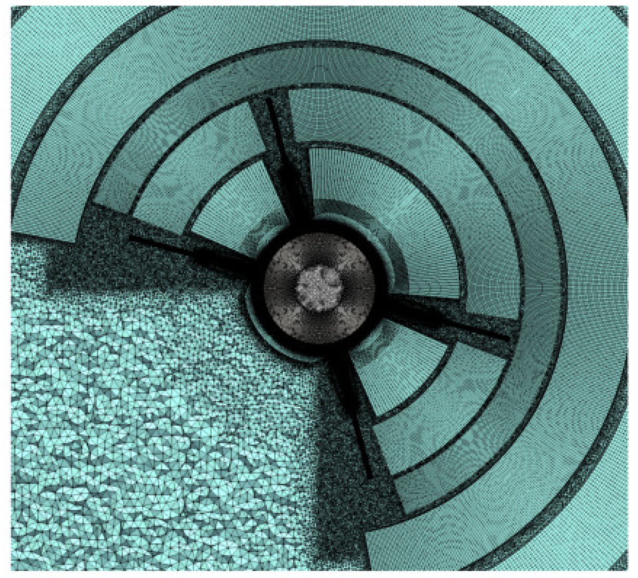
The computational domain is a typical external flow configuration. Thus, it consists of the missile wall surface, the far-field boundary and the fluid region between these two surfaces. The computational meshes are the ones shared by DLR during AVT-316 activity [6,8]. The meshes have a hybrid topology, where multiple types of elements co-exist. The number of hexahedral elements is maximized in the boundary layer and other near-body regions (see Figure 4). This topology is suggested for its superiority in vortex flows and used as common grids during AVT-316 studies [6,29,30]. Three mesh levels have been used in the study and are named as coarse, medium, and fine meshes. The numbers of nodes and elements in each level are shown in Table 4.
The boundary condition on the missile surface was defined as the no-slip adiabatic wall, where the velocity components were set to zero. The free stream flow variables were imposed via farfield type of boundary condition. Simulations were initialized from free stream values. The solver was run in steady mode, which enables local time-stepping for faster and stabilized convergence. The CFL number, which limits the time step in each individual computational cell, was chosen as 10. Line symmetric Gauss-Seidel (LSGS) was utilized for solutions of linear systems. For the inviscid flux discretization, the HLLC scheme was used [20]. Venkatakrishnan slope limiter [21,22] was employed to enable second-order spatial accuracy. The maximum time step is limited to s.
6. Results and Discussion
As mentioned in the description of the LK6E2 test case, the rolling moment loses its linearity at the aerodynamic roll angle () of 45° and total incidence angles () roughly between 17° and 21°. A series of simulations have been conducted to investigate the prediction performance of different turbulence models. We have tested variants of k--SST and k- turbulence models in this context. The results are presented in the following subsections. Firstly, we present the primary differences in the aerodynamic characteristics of the missile, as predicted by different turbulence models. Therefore, Section 6.1 covers an initial comparison between standard versions of k--SST and k-. Then, we aim to present the insight about the predicted flow features that lead to variation in the aerodynamic predictions in Section 6.2. The individual effects of alternative turbulent production formulations, rotational corrections, and compressibility and free shear corrections are presented in Section 6.3, Section 6.4 and Section 6.5, respectively.
6.1. Overall Aerodynamic Coefficients
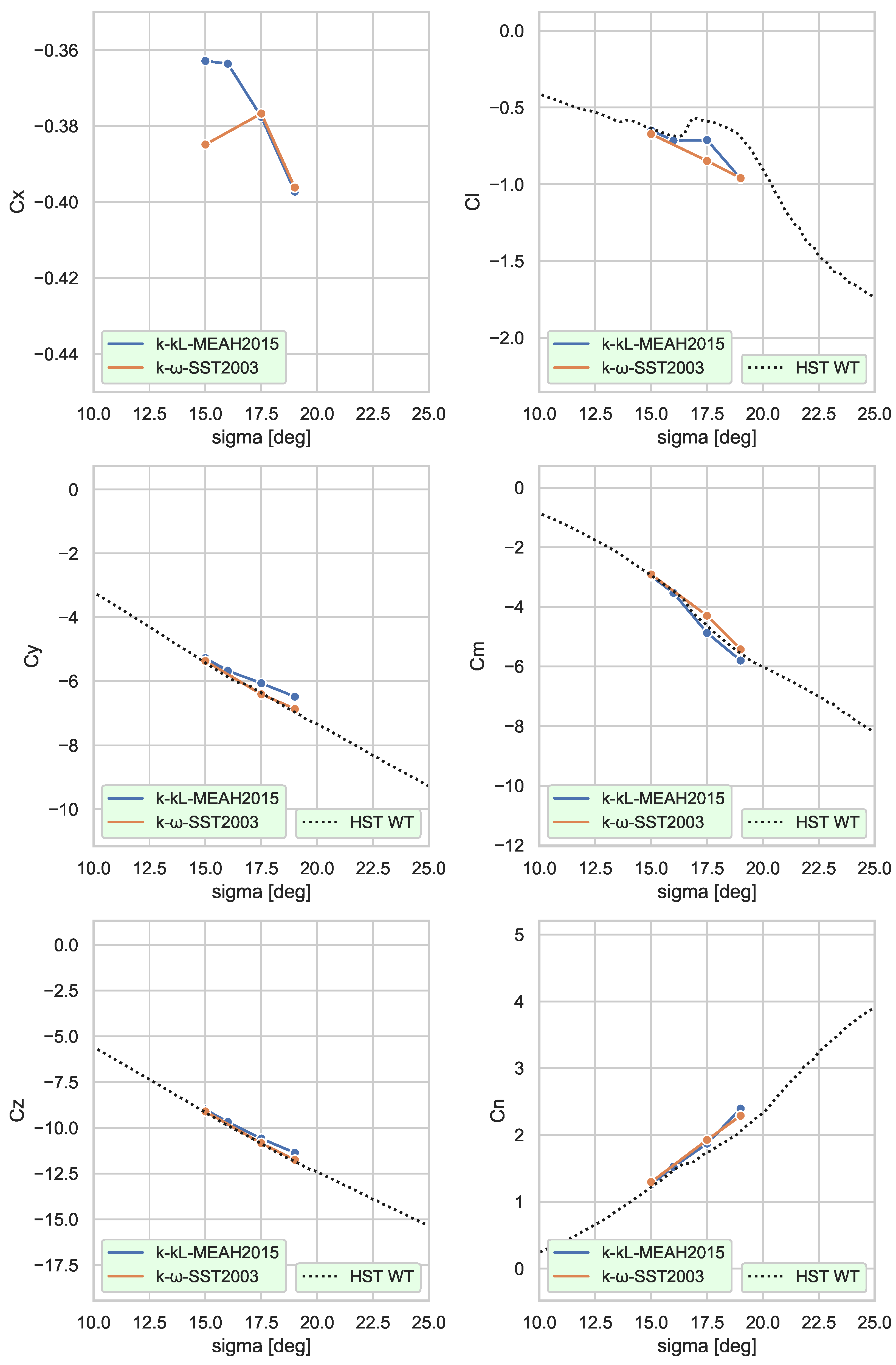
The variations of aerodynamic coefficients (, , , , , ) are reported at first. The results of the CFD simulations are plotted in Figure 5, together with experimental data collected in high-speed wind tunnel (HST) [6]. The experimental axial force coefficient () is not given in the plots because the data associated with it are not available. The behaviors of , , , coefficients against the incidence angle are similar amongst themselves, as these four coefficients are monotonic for the given flow condition range. Both RANS models can predict the slope within an acceptable margin. The difference between the RANS predictions and measurements increases for incidence angles larger than 16.0°. This condition corresponds to the location where a coefficient slope () changes its sign. At this angle of incidence, the results obtained with two turbulence models disagree substantially. It is clearly seen that the newly implemented k--MEAH2015 turbulence model captures the non-linearity and the sign change in the rolling moment slope, while the k--SST2003 model does not. Various research groups in the AVT-316 study reported the same discrepancies with various Spalart Allmaras and k- variants. Therefore, our k--MEAH2015 implementation stands out amongst the RANS simulations.
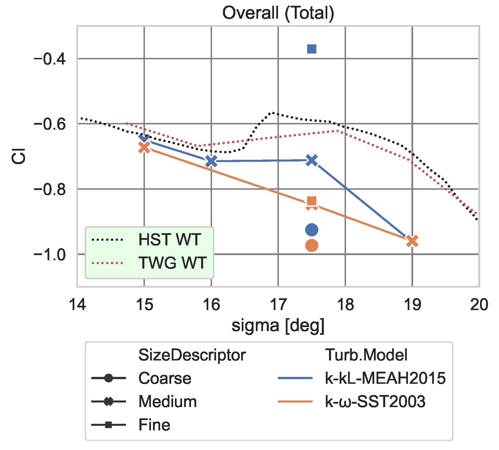
Figure 6 compares the numerical results with different turbulence models and mesh sizes with the wind tunnel data from the TWG and HST experiments [6]. The deviation from the experimental results for the computational data accumulated around can be observed more evidently. According to these results, the SST model cannot even sense the loss of linearity. This behavior is the same even when the fine mesh with 228 million elements is used. The k- model, on the other hand, makes much closer predictions, provided that the simulation is conducted with the medium or fine mesh. Despite the downside of not observing proper mesh independence up to this level of mesh density, the positive slope prediction of the rolling moment with medium and higher-density meshes is very encouraging.
The variation in rolling moment predictions is associated with the estimation of the interaction between the vortices and lifting surfaces of the missile. In order to investigate the origins of the large variation in the predictions made with different turbulence models, the rolling moment contributions from the wing and fin components are examined. Figure 7 illustrates the total rolling moment contribution of each wing and fin set. As shown in the figure, the difference in the contribution of fins to the rolling moment coefficient is insignificant and does not contribute to the slope change. On the contrary, the impact of wings on the rolling moment coefficient shows a much more sensible change in the behavior of the rolling moment coefficient with increasing incidence angle. The k- model precisely predicts the same trend we have observed in the overall rolling moment coefficient. We conclude that a shift in the rolling moment stems from the prediction of the flow over wings for incidence angles larger than 16°. The flow characteristic over the wings causes the non-linearity and slope reversal of the overall rolling moment.
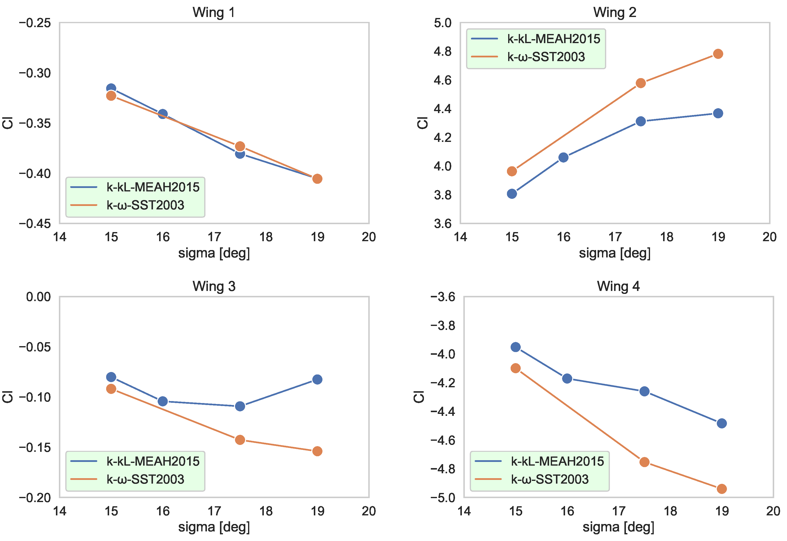
The analysis is extended by an examination of the contributions of individual wings, as illustrated in Figure 8. The contributions of wings numbered 1 and 3, which are approximately in line with the transverse component of relative flow velocity for the given aerodynamic roll angle (), are minimal compared to the other two wings. Though two turbulence models very differently predict the contribution of Wing 3 (leeward wing), a small portion of the difference is budgeted from Wing 3 (~0.03 out of ~0.20). The prediction differences of the wings numbered 2 and 4, which are located nearly horizontal with respect to flow, are much higher. Slopes of coefficient contributions by both wings are exposed to a significant change around the incidence angle of 16°. For Wing 2, this slope change occurs in the reverse direction. However, slope change in of Wing 4 has a more dominant influence, as the magnitude of the difference is more prominent. As a result, the slope change in the rolling moment contribution of Wing 4 is evaluated as the major effect on the shift in the overall rolling moment coefficient.
6.2. Wing Surface Flow Field
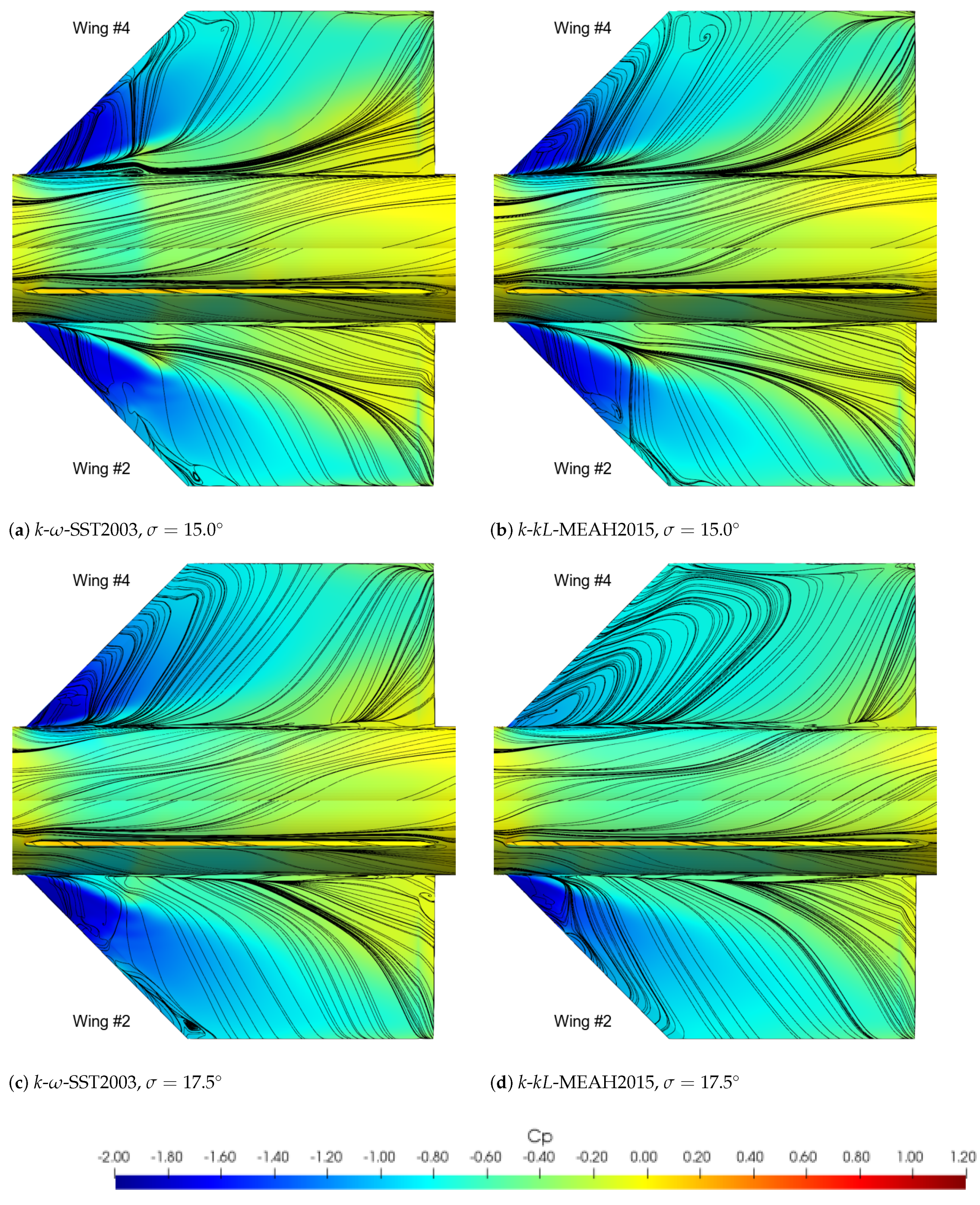
This section is devoted to investigating the difference in the estimation of the rolling moment contribution of the wings numbered 2 and 4, with different turbulence models, among which the latter is of more interest. For this purpose, the surface flow visualizations were applied to attain a better understanding of the flow features occurring simultaneously around this test case. Figure 9 illustrates the pressure distributions and streamlines extracted from the wall shear stress vectors on the leeward side of each wing. The flow incidence angles selected for this analysis are 15.0° and 17.5°, determined as the representative conditions “before” and “after” the rolling moment shift. At 15.0° incidence, the pressure fields on Wings 2 and 4 are fairly in balance, on which predictions of SST and k--MEAH2015 turbulence models agree.
On the contrary, the pressure distribution and vortex path on Wing 4 significantly change in the 17.5° incidence case in the k--MEAH2015 prediction. SST simulation, on the other hand, results in a completely different pressure distribution and vortex path for Wing 4. To summarize, the primary vortex of Wing 4 predicted by the k--MEAH2015 model travels towards more inboard, compared to the same vortex predicted by the k--SST2003 model. This pressure distribution difference explains why the k--MEAH2015 predictions are more in line with the experimental aerodynamic coefficients.
The discussion of vortex–surface interaction effects leads us to a more careful assessment of boundary layer characteristics. Figure 10 depicts the shear stress distributions on the same wings for cases with 15.0° and 17.5° incidence angles. It is observed in the k--MEAH2015 simulation that a large portion of Wing 4 is subject to a lower magnitude of shear stress at 17.5° incidence.
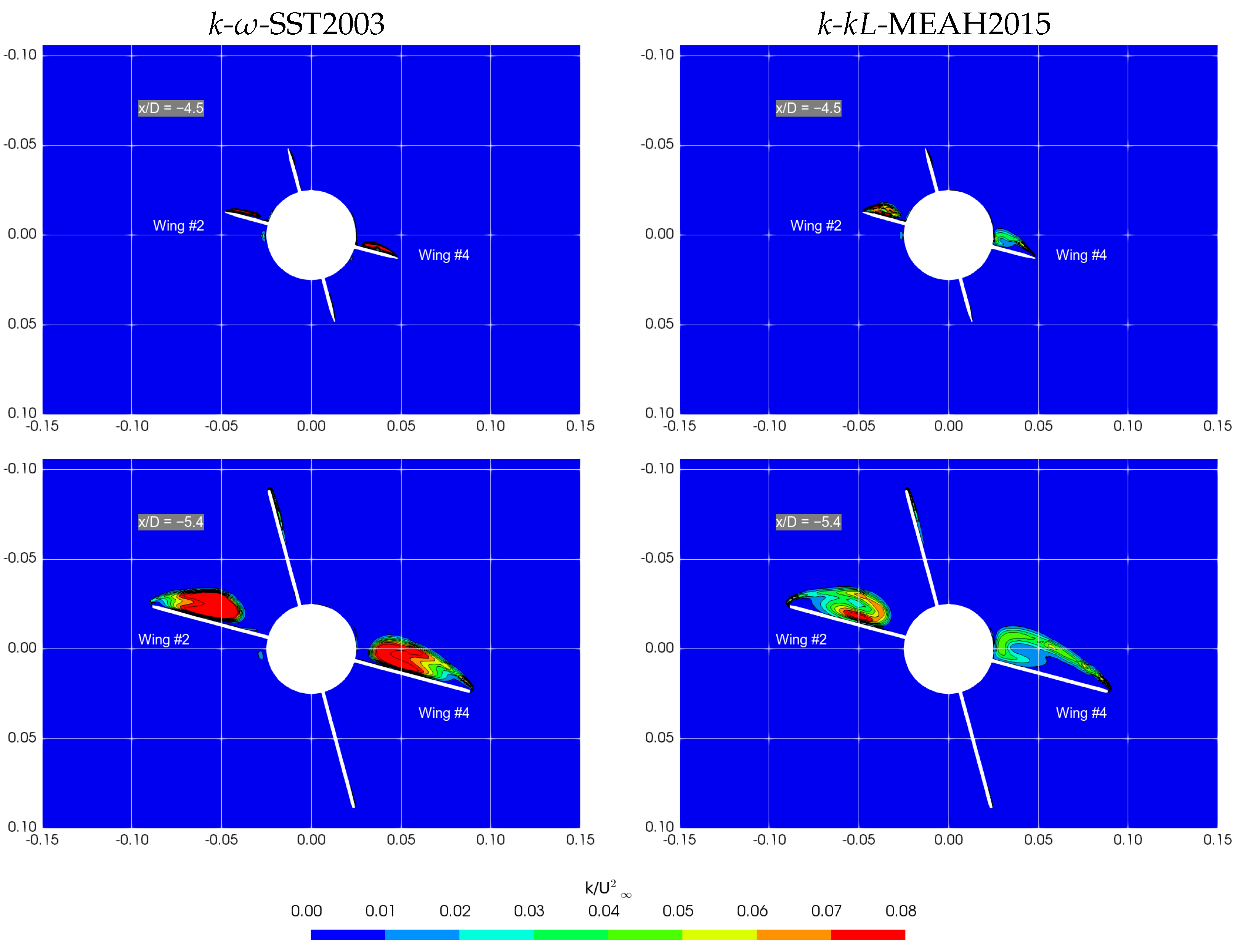
The explanation for this sudden change in the flow field within a few degrees of incidence is not straightforward. One explanation may be that the lower shear stress field is caused by the dissipation of the Wing 4 vortex at the 17.5° incidence. The turbulent kinetic energy (TKE) field in the mid-wing transverse plane is provided in Figure 11, in order to support this idea. As seen in this figure, the k--MEAH2015 model predicts a higher TKE in the shear layer formed at the edge of the vortex than in its core. The k--SST2003 model, on the other hand, predicts a much higher TKE. Low TKE at the vortex core allows preservation of the strength of the vortex; hence, larger vortices are observed in the k--MEAH2015 case.
Furthermore, the vortex over Wing 4 is larger than Wing 2 because of the angular orientation of the wing. Therefore, the edge of the Wing 4 vortex is in contact with the body in k--MEAH2015 results. Then, the TKE at the edge of Wing 4 vortex diffuses in the circumferential direction. Consequently, a large portion of the wing becomes subject to a less turbulent or “stabilized” flow field. In other words, as soon as the edge of the Wing 4 vortex reaches the missile body, the turbulent character of the vortex behind the wing decreases, and this causes dramatic changes in the flow field on the wing surface. Therefore, the behavior change across and , which is observed in Figure 9, is associated with the turbulent characteristics of the flow. The reason why the k--SST2003 model cannot resolve this effect is related to the unphysical prediction of the TKE field, starting from the leading edge of Wing 4. It was shown by the authors in another study that the k--SST2003 turbulence model fails to predict turbulent quantities accurately in a vortical flow field [14].
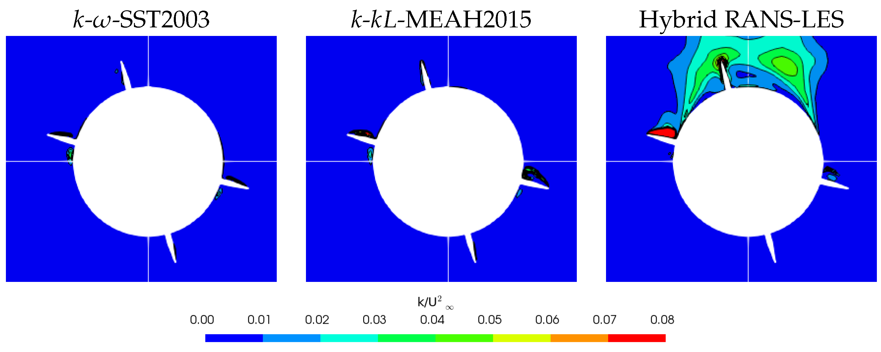
The turbulent kinetic energy field was also predicted with the hybrid RANS-LES method in another study conducted by others on the LK6E2 test case [43]. Due to the lack of experimental data, hybrid RANS-LES solutions are used as the reference results, as the turbulent content is resolved in these analyses. Figure 12 compares two different RANS methods with the hybrid RANS-LES computation. As evident in this figure, the turbulent kinetic energy fields in the leeward neighborhood of Wing 2 and Wing 4 are dissimilar, as predicted with hybrid RANS-LES. Wing 2 generates significantly higher turbulence, generated by the leading edge and spread over the leeward surface, while on Wing 4, the TKE level is significantly low and prominent on the vortex sheet. A similar distribution could be predicted with k--MEAH2015. The TKE prediction of k--SST2003 does not show the dissimilarity between the wings numbered 2 and 4. For this reason, this model does not capture the difference in the pressure and wall shear stress fields shown previously in Figure 9 and Figure 10. Neither RANS model can predict the turbulence generated by the forebody of the missile. However, this fact does not cause critical consequences on aerodynamic coefficients, since this turbulent field does not influence Wings 2 and 4.
It should be noted that the k- model does not provide any measurable benefit or weakness over the standard models at low vorticity flows or at flows where no significant vortex–body interactions are observed. From the engineering perspective, accurate predictions of the vortex characteristics are often insignificant, since they often do not alter the aerodynamic force predictions.
We have shown that the k- model is significantly better in predicting vortical flows. If those vortices interact with the body, the utilization of the k- model is advisable. The results show that, albeit the standard model produces significantly less TKE, further developments in the model may improve the vortex simulation capability.
6.3. Improvements via Alternative Turbulent Production Formulations
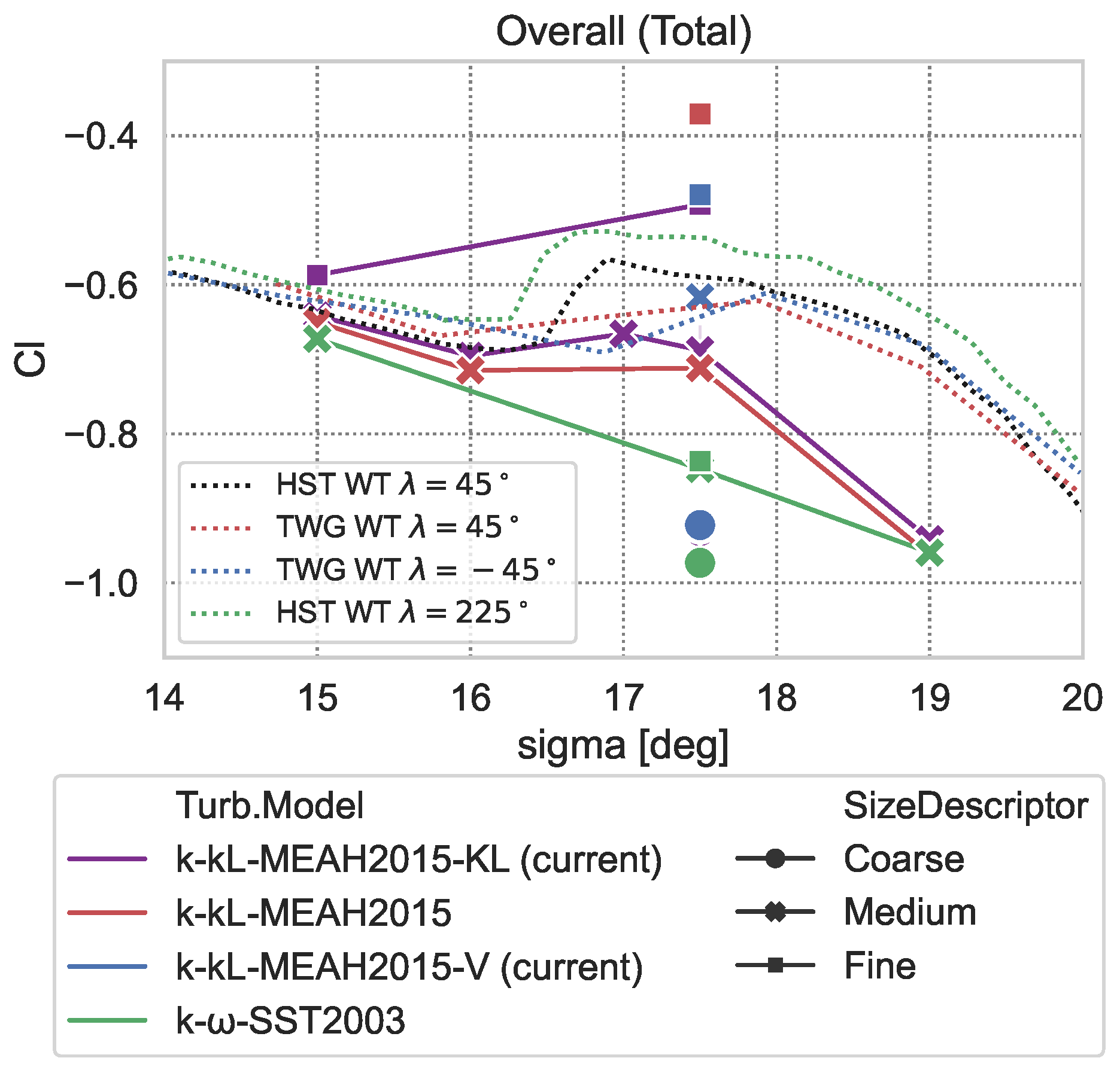
The key modification, with respect to the original k--MEAH2015, is the formulation of the turbulence production. The details of this modification were already provided in Section 4.2. In this section, simulations with the original k--MEAH2015 turbulence model are also presented. Figure 13 summarizes the rolling moment coefficient data obtained with both k- variants, in comparison with the reference wind tunnel measurement data. Both variants performed with inadequate accuracy when coarse mesh (36 mil. elements) was used. For higher-density meshes, both models were able to catch the non-linearity. However, k--MEAH2015-KL resulted in data closer to the experimental with medium mesh (113 mil. elements). Additionally, the sign change of the rolling moment slope was not captured by k--MEAH2015 with this level of mesh. Though both fine mesh results showed an overshoot, the k--MEAH2015-KL result was much closer to the experimental data. Moreover, k--MEAH2015-KL performed better, in terms of mesh independence. The difference between medium and fine mesh results was almost half of the same set of k--MEAH2015 results.
For 17.5 degree incidence, k--MEAH2015-V provided better agreement with physical data with medium mesh. On the other hand, the fine mesh results of k--MEAH2015-V and k--MEAH2015-KL are so close to each other. Therefore, the evaluations made for k--MEAH2015-KL in the previous paragraph are also valid for k--MEAH2015-V.
Mesh sensitivity is evaluated along with the experimental uncertainty. Figure 13 also shows the extended experimental data obtained from symmetric attitude conditions [44]. Mesh dependence is observed at in the results of all variants of the k- model, even between the medium and fine levels. However, the improved models (k--MEAH2015-KL and k--MEAH2015-V) show less sensitivity. Indeed, the difference between the medium and fine mesh results for these models is comparable to experimental uncertainty.
The improvement obtained from the turbulence production formulation is interesting. Our results show that all formulations yield the same moment coefficient behavior as the mesh is refined further from the medium mesh. This is expected, since the k- model provides better length scale estimates as the mesh gets finer, and no corrections are required as the length scale is resolved. In practice, the mesh densities finer than those given in this study are not applicable, due to concerns about computational resources. Our improvements provided a better estimation for medium and finer meshes.
6.4. Influence of Rotation Corrections on the SST and k- Computations
As shown in several recent studies on external aerodynamic flow with vortex development [31,45,46,47,48], the RANS models result in inaccurate predictions of vortex dynamics, as a result of over-prediction of turbulent quantities. Spalart suggests that this shortcoming arises since the vortex effects were not included in the development and calibration procedures of turbulence models [45]. Some of the recent research has focused on the performance of rotational corrections applied to the RANS models, where a certain level of improvements have been achieved for the prediction of downstream vortical flow properties [31,45,49]. Nevertheless, the influence of rotational corrections has not been clearly identified for the vortex separation. This section of the paper focuses on whether the rotational corrections cause any improvement in the RANS predictions of vortex separation on transonic missile wings. In order to assess the capabilities of rotational corrections in the reduction of the excessive turbulence production at the vortex core, the rotation/curvature (RC) [35] type correction was applied to the k--SST2003 and k--MEAH2015-KL turbulence models.
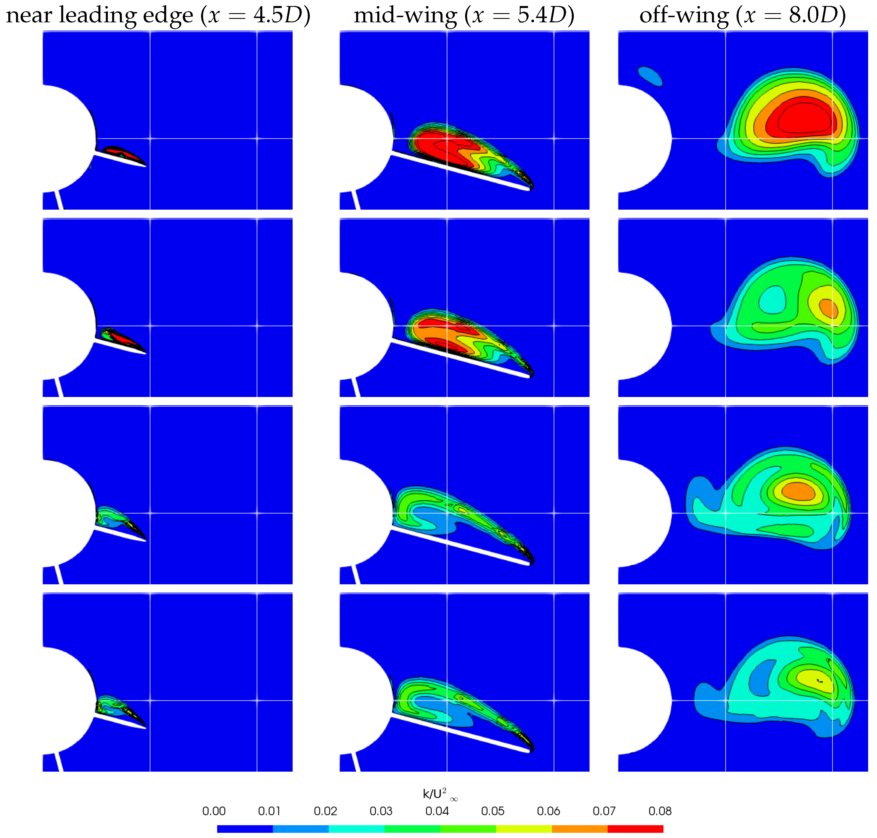
The LK6E2 test case was first run using the RC correction-applied k--SST2003 model, which was expected to provide a reduction of computed turbulent quantities within the vortex core. However, this functionality does not unconditionally work as the vortex developed on Wing 4. As shown in Figure 14, the RC correction comes across with a limited reduction in the computed turbulent content near the leading edge. As observed in this case, the turbulent kinetic energy diminishes down to the level of what k--MEAH2015-KL computes for only matured zones of the vortex, e.g., downstream of the wing (). In the vicinity of the wing surface, however, TKE fields and, consequently, the vortex sizes computed by k--SST2003 with and without RC correction are close and significantly different from the k--MEAH2015-KL case, which best agrees with the experimental results. Since the vortex flow field in the vicinity of the wing surfaces does not change significantly, RC correction does not improve the prediction of vortex separation and, hence, the rolling moment coefficient (Table 5).
The RC was also tested for the k--MEAH2015-KL turbulence model. The effect of RC on predicted TKE is found to be marginal within the wing surface. Parallel to this observation, there is a slight difference in the rolling moments coefficient computed by k--MEAH2015-KL with and without RC correction. Likewise to the k--SST2003 case, the effect of the RC correction is more pronounced for the matured vortex at the off-wing region. As a result, no significant contribution of RC correction is observed with regard to the leading edge vortex separation. The resultant rolling moment coefficients calculated using both turbulence models with and without RC correction are presented in Table 5. As seen in this table, the application of k--MEAH2015-KL is recommended, regardless of whether RC is applied.
Our study showed that the vortical corrections (i.e., RC correction) do not improve the SST results in a case containing leading edge vortex separation, contrary to previous studies claiming a solution to the over-dissipation issue for separated vortices. As is known, the primary mechanism of the vortical corrections is to reduce the turbulence production at the regions where the vorticity magnitude is dominant over the strain invariant, i.e., the vortex cores. However, the flow field over the wings of LK6E2 is dependent on the turbulence initiated at the leading edges. As the vortices are not mature enough to possess a well-developed vortex core at this location, the vortical corrections cannot properly detect the vortex core and, hence, cannot provide the desired effect. The k- turbulence model inherently computes less turbulence in the vortex core, compared to the vortex sheet; therefore, this model is concluded as a powerful method in predicting such flow features.
6.5. Influence of Compressibility and Free Shear Corrections
Compressibility and free shear corrections may be significant modifications to enhance the performance of RANS models in off-body zones. Both corrections are usually applied together, as they make up jet correction. The influence of these corrections has been investigated for the LK6E2 problem to establish a complete modeling scheme. The primary function of compressibility correction is to reduce turbulence production to account for local compressibility. On the other hand, free shear correction is active on the diffusion term in the TKE transport equation. The influence of the jet corrections was previously shown by others for much simpler jet flow problems [12], yet this is the first time they have been tested for a large-scale vortex separation problem. In this regard, the k--MEAH2015-KL turbulence model with a number of combinations of jet correction options has been analyzed for the LK6E2 problem.
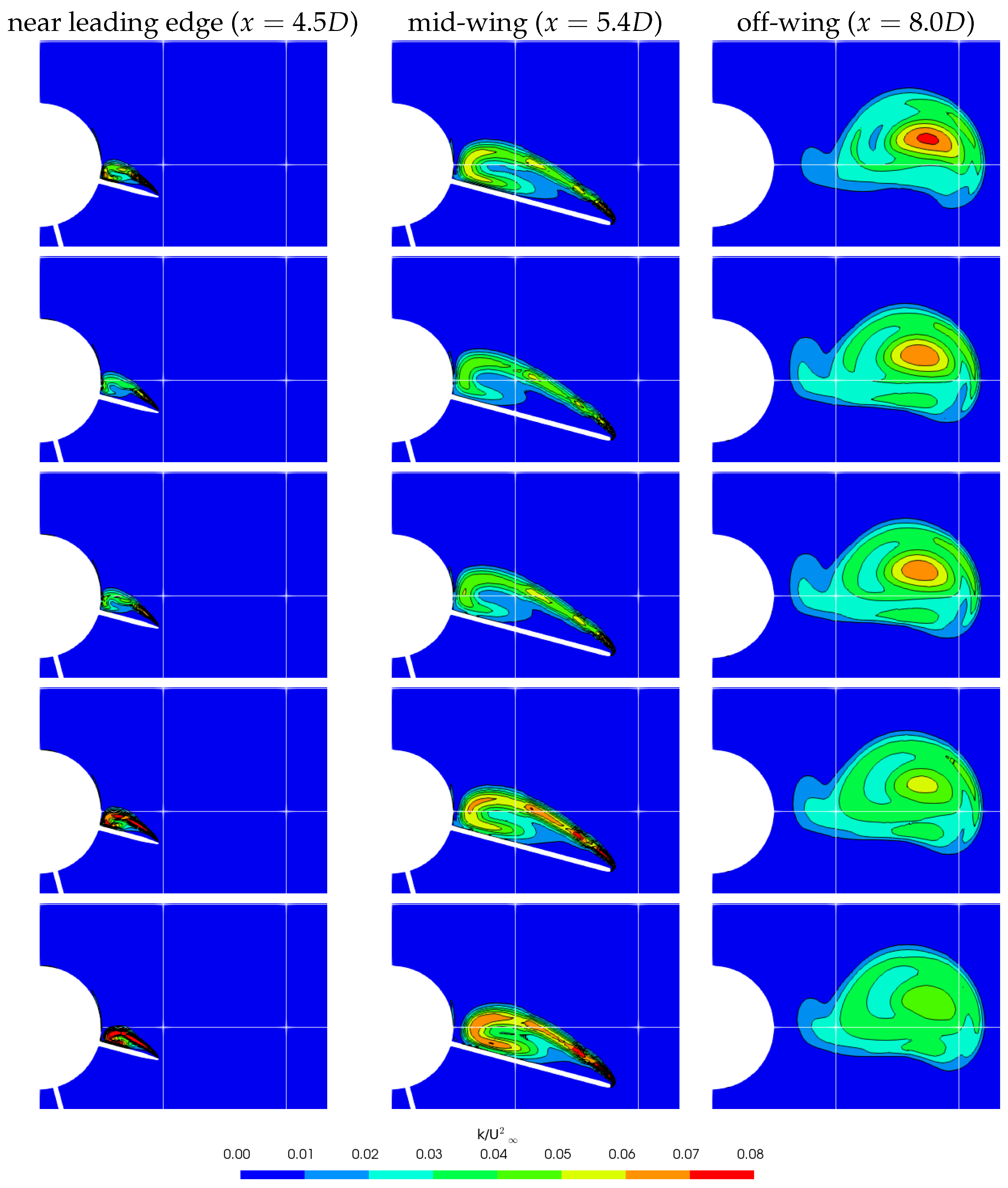
The results presented in the other sections of the paper belong to the simulations, with Wilcox compressibility correction combined with free shear correction. In Figure 15, TKE predictions obtained with the same method are presented in comparison to the results of (i) modified Wilcox formulation described by Abdol-Hamid [12], (ii) Sarkar’s method with free shear correction, (iii) free shear method with no compressibility correction, and (iv) no jet correction. For all methods, TKE does not reach as extreme levels as k--SST2003 predicts. However, the differences in TKE fields may result in crucial differences in the integrated rolling moment, as shown in Table 6. Obviously, any of the compressibility corrections enhance the results to agree with the experimental result much better than the results obtained without compressibility correction. This is achieved by a more realistically computed TKE field starting from the leading edge. The choice of compressibility correction method plays an insignificant role in the overall results. By the difference between only the free shear correction and the no-correction results, it can be inferred that free shear correction plays a minor role in the prediction of the TKE and, thus, the integrated rolling moment. By a similar assessment, the use of the original Wilcox correction, which defines turbulent cut-off Mach number as 0.10, provides a slightly more accurate result than the Abdol-Hamid’s modification, which suggests the use of the same parameter as 0.17. After all, enabling compressibility correction with Wilcox’s original parameters is recommended for computations of vortex separation problems to enhance the performance of the k--MEAH2015-KL turbulence model.
This study verifies the necessity of jet corrections for the k- turbulence model in the cases of compressible flow problems, as also suggested by Abdol-Hamid et al. [12]. Our study reveals that a further marginal improvement can be achieved by using Wilcox’s original parameters, instead of Abdol-Hamid’s modified parameters.
7. Conclusions
This paper presents the CFD results obtained with the k--MEAH2015 turbulence model for a flow field of a generic bank-to-turn concept transonic missile. The flow condition introduced a vortex separation on the wings, which is challenging to capture accurately for most of the RANS turbulence models. The computed flow variables in the leeward vortices on the wings strongly depend on the employed turbulence model. Likewise, the vortex paths are influenced by computed turbulent characteristics. The variation in the flow field, depending on the turbulence model, affects the computed rolling moment coefficient. Thus, the sign of the rolling moment derivative, with respect to the incidence angle, is altered. With respect to the experimental aerodynamic results, the k- turbulence model calculates much more credible predictions, compared to other turbulence models, such as SST.
The results of the k- turbulence model show that a statistical RANS model can model the vortex separation with adequate accuracy, contrary to previous studies suggesting higher-order models, such as the hybrid RANS/LES. k- turbulence model, and it stands out amongst the statistical turbulence models for the vortex flow problems similar to that studied in the current paper, as no other patch or remedy has been shown to improve another statistical turbulence model. For instance, rotational corrections do not enhance the performance of other failing turbulence models in the prediction of vortex separation physics.
The variants of the k- turbulence model family have been developed and tested for this complex flow problem. The Kato-Launder and vorticity-based production formulations (k--MEAH2015-KL and k--MEAH2015-V) have been shown to be better options than the original version, as they provide more accurate results and less sensitivity, with respect to mesh resolution. Apart from this, it has been shown that jet flow corrections involving compressibility and free shear corrections should be applied when the k- turbulence model is used. Compressibility correction especially plays an important role in avoiding excessive turbulent content prediction, which may lead to the inaccurate calculation of integrated aerodynamic coefficients. The turbulent cut-off Mach number parameter affects the effectiveness of the compressibility correction. The value of this parameter should be chosen as 0.10, as Wilcox described.
The AVT-316 study [8] revealed that popular turbulence models fall short in vortical flows and vortex–body interactions. The authors also showed that the major problem associated with this inaccuracy stems from excessive turbulence production at the vortex core. We suggest a state-of-the-art turbulence model and offer further improvements on this model to eliminate these shortcomings. Finally, we provide a refined methodology to be employed in accurate simulations in compressible vortical flows, which is one of the major outcomes of this study.
This problem often arises in missile development studies. As the NATO STO AVT-316 study demonstrated, vortices generated from the tips of lifting surfaces interact with the control surfaces that disturb the roll characteristics. These problems are often overlooked in CFD simulation and can only be captured with expensive wind tunnel tests. Our improved model improves the confidence in RANS-based CFD solutions in these flight regions. Please note that the improved k- turbulence model is computationally much cheaper than hybrid RANS/LES simulations.
Author Contributions
Both authors (E.D. and Ö.U.B.) equally contributed to this research paper. Both authors (E.D. and Ö.U.B.) have read and agreed to the published version of the manuscript. All authors have read and agreed to the published version of the manuscript.
Funding
This research received no external funding.
Data Availability Statement
Data sharing not applicable.
Acknowledgments
The authors would like thank the fellow participants of the NATO STO AVT-316 research group for their collaboration during the panel group activity. The contribution of Christian Schnepf in constructing the shared computational meshes is greatly appreciated. It is acknowledged that the numerical calculations reported in this paper were partially performed at TUBITAK ULAKBIM, High Performance and Grid Computing Center (TRUBA resources).
Conflicts of Interest
The authors declare no conflict of interest.
References
- Cummings, R.M.; Forsythe, J.R.; Morton, S.A.; Squires, K.D. Computational challenges in high angle of attack flow prediction. Prog. Aerosp. Sci. 2003, 39, 369–384. [Google Scholar] [CrossRef]
- Luckring, J.M.; Boelens, O.J.; Schmidt, S.; Eloot, K.; van Hoydonck, W.; Simonsen, C.D.; Bordier, L.; Deck, S.; Visonneau, M.; Abdel-Maksoud, M.; et al. Reliable Prediction of Separated Flow Onset and Progression for Air and Sea Vehicles; Technical Report TR-AVT-183; NATO Science and Technology Organization: Neuilly-sur-Seine, France, 2017. [Google Scholar]
- Rizzi, A.; Luckring, J.M. Historical development and use of CFD for separated flow simulations relevant to military aircraft. Aerosp. Sci. Technol. 2021, 117, 106940. [Google Scholar] [CrossRef]
- Taylor, N. Separated Flow: Some Challenges and Research Priorities for Missile Aerodynamics. In Separated Flow: Prediction, Measurement and Assessment for Air and Sea Vehicles; NATO Science and Technology Organization: Neuilly-sur-Seine, France, 2019; number MP-AVT-307-23. [Google Scholar]
- Taylor, N.; McGowan, G.; Anderson, M.; Schnepf, C.; Richter, K.; Tormalm, M.; Loupy, G.; Michel, V.; Jeune, C.; Shaw, S.; et al. The Prediction of Vortex Interactions on a Generic Missile Configuration Using CFD: Current Status of Activity in NATO AVT-316. In Separated Flow: Prediction, Measurement and Assessment for Air and Sea Vehicles; NATO Science and Technology Organization: Neuilly-sur-Seine, France, 2019; number MP-AVT-307-24. [Google Scholar]
- Schnepf, C.; Anderson, M.; DeSpirito, J.; Dikbaş, E.; Cesur, İ.S.; Tormalm, M. Comparisons of Predicted and Measured Aerodynamic Characteristics of the DLR LK6E2 Missile Airframe. In Proceedings of the AIAA SciTech 2022 Forum, San Diego, CA, USA, 3–7 January 2022. [Google Scholar] [CrossRef]
- De Spirito, J.; Tormalm, M.H.; Schnepf, C.; Loupy, G.J.; Dikbaş, E.; Cesur, İ.S. Comparisons of Predicted and Measured Aerodynamic Characteristics of the DLR LK6E2 Missile Airframe (Scale Resolving). In Proceedings of the AIAA SciTech 2022 Forum, San Diego, CA, USA, 3–7 January 2022. [Google Scholar] [CrossRef]
- Luckring, J.M. Vortex Interaction Effects Relevant to Military Air Vehicle Performance; Technical Report TR-AVT-316; NATO Science and Technology Organization: Neuilly-sur-Seine, France, 2022; to be published. [Google Scholar]
- Menter, F.R.; Egorov, Y. Revisiting the turbulent scale equation. In IUTAM Symposium on One Hundred Years of Boundary Layer Research; Springer: Berlin/Heidelberg, Germany, 2006; pp. 279–290. [Google Scholar] [CrossRef]
- Menter, F.R.; Egorov, Y. The scale-adaptive simulation method for unsteady turbulent flow predictions. part 1: Theory and model description. Flow Turbul. Combust. 2010, 85, 113–138. [Google Scholar] [CrossRef]
- Abdol-Hamid, K.S. Assessments of-turbulence model based on Menter’s modification to Rotta’s two-equation model. Int. J. Aerosp. Eng. 2015, 2015, 987682. [Google Scholar] [CrossRef]
- Abdol-Hamid, K.S.; Carlson, J.R.; Rumsey, C.L. Verification and Validation of the k-kL Turbulence Model in FUN3D and CFL3D Codes. In Proceedings of the 46th AIAA Fluid Dynamics Conference, Washington, DC, USA, 13–17 June 2016. [Google Scholar] [CrossRef]
- Dikbaş, E.; Baran, Ö.U. Implementation and verification of k-kL turbulence model. In Proceedings of the 11th Ankara International Aerospace Conference, Ankara, Türkiye, 8–10 September 2021. number AIAC-2021-129. [Google Scholar]
- Dikbaş, E.; Baran, Ö.U. Implementation, verification and assessment of vortex capturing capabilities of k-kL turbulence model. J. Therm. Sci. Technol. 2022, 42, 113–122. [Google Scholar] [CrossRef]
- Beresh, S.J.; Henfling, J.F.; Spillers, R.W. Planar Velocimetry of a Fin Trailing Vortex in Subsonic Compressible Flow. AIAA J. 2009, 47, 1730–1740. [Google Scholar] [CrossRef]
- Beresh, S.J.; Henfling, J.F.; Spillers, R.W. Meander of a fin trailing vortex and the origin of its turbulence. Exp. Fluids 2010, 49, 599–611. [Google Scholar] [CrossRef]
- Beresh, S.J.; Henfling, J.F.; Spillers, R.W. Turbulence of a fin trailing vortex in subsonic compressible flow. AIAA J. 2012, 50, 2609–2622. [Google Scholar] [CrossRef]
- Luke, E.A.; Tong, X.; Chamberlein, R. FlowPsi Source Code, Version 1-0-p4. Available online: https://github.com/libm3l/FlowPsi/tree/flowPsi-1-0-p4 (accessed on 15 January 2023).
- Luke, E.A.; Tong, X.; Chamberlain, R. FlowPsi: An Ideal Gas Flow Solver-The User Guide. Available online: https://github.com/libm3l/FlowPsi/tree/flowPsi-1-0-p4/guide (accessed on 15 January 2023).
- Toro, E.F.; Spruce, M.; Speares, W. Restoration of the contact surface in the HLL-Riemann solver. Shock Waves 1994, 4, 25–34. [Google Scholar] [CrossRef]
- Venkatakrishnan, V. On the Accuracy of Limiters and Convergence to Steady State Solutions. In Proceedings of the 31st Aerospace Sciences Meeting, Reno, NV, USA, 11–14 January 1993. [Google Scholar] [CrossRef]
- Venkatakrishnan, V. Convergence to steady state solutions of the Euler equations on unstructured grids with limiters. J. Comput. Phys. 1995, 118, 120–130. [Google Scholar] [CrossRef]
- Barth, T.; Jespersen, D. The Design and Application of Upwind Schemes on Unstructured Meshes. In Proceedings of the 27th Aerospace Sciences Meeting, Reno, NV, USA, 9–12 January 1989. [Google Scholar] [CrossRef]
- Menter, F.R.; Kuntz, M.; Langtry, R. Ten years of industrial experience with the SST turbulence model. In Turbulence, Heat and Mass Transfer 4; Begell House: New York, NY, USA, 2003; pp. 625–632. [Google Scholar]
- Rotta, J. Statistische Theorie nichthomogener Turbulenz. Z. Phys. 1951, 129, 547–572. [Google Scholar] [CrossRef]
- Menter, F.R.; Schütze, J.; Kurbatskii, K.A.; Gritskevich, M.; Garbaruk, A. Scale-Resolving Simulation Techniques in Industrial CFD. In Proceedings of the 6th AIAA Theoretical Fluid Mechanics Conference, Honolulu, HI, USA, 27–30 June 2011. [Google Scholar] [CrossRef]
- Abdol-Hamid, K.S. Development of kL-Based Linear, Nonlinear, and Full Reynolds Stress Turbulence Models. In Proceedings of the AIAA SciTech 2019 Forum, San Diego, CA, USA, 7–11 January 2019. [Google Scholar] [CrossRef]
- Rumsey, C.L. Turbulence Modeling Resource. 2022. Available online: https://turbmodels.larc.nasa.gov (accessed on 7 September 2022).
- Dikbaş, E.; Schnepf, C.; Tormalm, M.; Anderson, M.; Shaw, S.; DeSpirito, J.; Loupy, G.; Barakos, G.; Boychev, K.; Toomer, C.; et al. The Influence of the Computational Mesh on the Prediction of Vortex Interactions about a Generic Missile Airframe. In Proceedings of the AIAA SciTech 2022 Forum, San Diego, CA, USA, 3–7 January 2022. [Google Scholar] [CrossRef]
- Anderson, M.; Cooley, K.; DeSpirito, J.; Schnepf, C. The Influence of the Numerical Scheme in Predictions of Vortex Interaction about a Generic Missile Airframe. In Proceedings of the AIAA SciTech 2022 Forum, San Diego, CA, USA, 3–7 January 2022. [Google Scholar] [CrossRef]
- Shaw, S.; Anderson, M.; Barakos, G.; Boychev, K.; Dikbaş, E.; DeSpirito, J.; Loupy, G.; Schnepf, C.; Tormalm, M. The Influence of Modelling in Predictions of Vortex Interactions About a Generic Missile Airframe: RANS. In Proceedings of the AIAA SciTech 2022 Forum, San Diego, CA, USA, 3–7 January 2022. [Google Scholar] [CrossRef]
- Loupy, G.J. A Focused Study into the Prediction of Vortex Formation about Generic Missile and Combat Aircraft Airframes. In Proceedings of the AIAA SciTech 2022 Forum, San Diego, CA, USA, 3–7 January 2022. [Google Scholar] [CrossRef]
- Kato, M.; Launder, B.E. The modelling of turbulent flow around stationary and vibrating square cylinders. In Proceedings of the Ninth Symposium on “Turbulent Shear Flows”, Kyoto, Japan, 16–18 August 1993. [Google Scholar]
- Dacles-Mariani, J.; Zilliac, G.G.; Chow, J.S.; Bradshaw, P. Numerical/experimental study of a wingtip vortex in the near field. AIAA J. 1995, 33, 1561–1568. [Google Scholar] [CrossRef]
- Shur, M.L.; Strelets, M.K.; Travin, A.K.; Spalart, P.R. Turbulence modeling in rotating and curved channels: Assessing the Spalart-Shur correction. AIAA J. 2000, 38, 784–792. [Google Scholar] [CrossRef]
- Smirnov, P.E.; Menter, F.R. Sensitization of the SST turbulence model to rotation and curvature by applying the Spalart-Shur correction term. J. Turbomach. 2009, 131, 041010. [Google Scholar] [CrossRef]
- Bush, R.H.; Chyczewski, T.S.; Duraisamy, K.; Eisfeld, B.; Rumsey, C.L.; Smith, B.R. Recommendations for Future Efforts in RANS Modeling and Simulation. In Proceedings of the AIAA SciTech 2019 Forum, San Diego, CA, USA, 7–11 January 2019. [Google Scholar] [CrossRef]
- Wilcox, D.C. Dilatation-dissipation corrections for advanced turbulence models. AIAA J. 1992, 30, 2639–2646. [Google Scholar] [CrossRef]
- Sarkar, S.; Erlebacher, G.; Hussaini, M.Y.; Kreiss, H.O. The analysis and modelling of dilatational terms in compressible turbulence. J. Fluid Mech. 1991, 227, 473–493. [Google Scholar] [CrossRef]
- Menter, F.R. Improved Two-Equation k-ω Turbulence Models for Aerodynamic Flows; Technical Report NASA-TM-103975; NASA Ames Research Center: Moffett Field, CA, USA, 1992.
- Cheng, Y.; Lien, F.S.; Yee, E.; Sinclair, R. A comparison of large eddy simulations with a standard k-ϵ Reynolds averaged Navier-Stokes model for the prediction of a fully developed turbulent flow over a matrix of cubes. J. Wind. Eng. Ind. Aerodyn. 2003, 91, 1301–1328. [Google Scholar] [CrossRef]
- Menter, F.R.; Smirnov, P.E.; Liu, T.; Avancha, R. A one-equation local correlation-based transition model. Flow Turbul. Combust. 2015, 95, 583–619. [Google Scholar] [CrossRef]
- DeSpirito, J.; Schnepf, C.; Dikbaş, E.; Anderson, M.; Loupy, G.; Tormalm, M. Predictions of Vortex Interactions for LK6E2—Part I. In Vortex Interaction Effects Relevant to Military Air Vehicle Performance; Number TR-AVT-316; NATO Science and Technology Organization: Neuilly-sur-Seine, France, 2023; Chapter 8; to be published. [Google Scholar]
- Schnepf, C.; DeSpirito, J.; Anderson, M.; Dikbaş, E.; Loupy, G.; Baran, Ö.U. Predictions of Vortex Interactions for LK6E2—Part II. In Vortex Interaction Effects Relevant to Military Air Vehicle Performance; Number TR-AVT-316; NATO Science and Technology Organization: Neuilly-sur-Seine, France, 2023; Chapter 9; to be published. [Google Scholar]
- Spalart, P.R.; Garbaruk, A.V. The predictions of common turbulence models in a mature vortex. Flow Turbul. Combust. 2019, 102, 667–677. [Google Scholar] [CrossRef]
- Asnaghi, A.; Svennberg, U.; Bensow, R.E. Large eddy simulations of cavitating tip vortex flows. Ocean. Eng. 2020, 195, 106703. [Google Scholar] [CrossRef]
- Landa, T.; Klug, L.; Radespiel, R.; Probst, S.; Knopp, T. Experimental and Numerical Analysis of a Streamwise Vortex Downstream of a Delta Wing. AIAA J. 2020, 58, 2857–2868. [Google Scholar] [CrossRef]
- Werner, M.; Schütte, A.; Weiss, S. Turbulence Model Effects on the Prediction of Transonic Vortex Interaction on a Multi-Swept Delta Wing. In Proceedings of the AIAA SciTech 2022 Forum, San Diego, CA, USA, 3–7 January 2022. [Google Scholar] [CrossRef]
- Asnaghi, A.; Svennberg, U.; Bensow, R.E. Evaluation of curvature correction methods for tip vortex prediction in SST k-ω turbulence model framework. Int. J. Heat Fluid Flow 2019, 75, 135–152. [Google Scholar] [CrossRef]
Figure 1.
LK6E2 model geometry and axes definition (Adapted with permission from Ref. [6]. Copyright ©2022 by German Aerospace Center).
Figure 1.
LK6E2 model geometry and axes definition (Adapted with permission from Ref. [6]. Copyright ©2022 by German Aerospace Center).

Figure 2.
LK6E2 flow topology (, , , ), (Adapted with permission from Ref. [6]. Copyright ©2022 by German Aerospace Center.)
Figure 2.
LK6E2 flow topology (, , , ), (Adapted with permission from Ref. [6]. Copyright ©2022 by German Aerospace Center.)

Figure 3.
Computational and experimental data at LK6E2 test conditions (, ), Reprinted with permission from Ref. [6]. Copyright ©2022 by German Aerospace Center)
Figure 3.
Computational and experimental data at LK6E2 test conditions (, ), Reprinted with permission from Ref. [6]. Copyright ©2022 by German Aerospace Center)

Figure 4.
Cross-sectional view of mesh topology.

Figure 5.
Aerodynamic coefficients vs. incidence angle, ; , , ; medium mesh.

Figure 6.
Rolling moment coefficient predictions in comparison with experimental data; , , .

Figure 7.
Rolling moment coefficient contributions of wing and fins; , , .

Figure 8.
Individual wing contributions to rolling moment coefficient;, , .

Figure 9.
Streamlines and static pressure distributions on leeward sides of Wings 2 and 4; , , .

Figure 10.
Comparisons of Wing 2 and 4 leeward skin friction distributions; , , ; SOmega production.
Figure 10.
Comparisons of Wing 2 and 4 leeward skin friction distributions; , , ; SOmega production.

Figure 11.
Normalized turbulent kinetic energy field in mid-wing transverse plane; , , .

Figure 12.
Comparison of RANS methods with available hybrid RANS/LES computation; , , , .

Figure 13.
Rolling moment coefficient predictions in comparison with experimental data; , , .

Figure 14.
Normalized turbulent kinetic energy field in transverse planes; , , ; Row 1: k--SST2003, Row 2: k--SST2003-RC, Row 3: k--MEAH2015-KL, Row 4: k--MEAH2015-KL-RC.
Figure 14.
Normalized turbulent kinetic energy field in transverse planes; , , ; Row 1: k--SST2003, Row 2: k--SST2003-RC, Row 3: k--MEAH2015-KL, Row 4: k--MEAH2015-KL-RC.

Figure 15.
Comparison of TKE field obtained with different compressibility correction settings; , , ; Kato-Launder production; Row 1: modified Wilcox with free shear correction (described by Abdol-Hamid et al. [12]), Row 2: Wilcox with free shear correction, Row 3: Sarkar with free shear correction, Row 4: only free shear correction, Row 5: no correction


Table 1.
LK6E2 test case flow conditions.
| Flow Similitude Quantities | Physical Quantities | ||||
|---|---|---|---|---|---|
| Mach number | static pressure | 47075 Pa | |||
| Reynolds number | static temperature | K | |||
| incidence angle | – | velocity | m/s | ||
| roll angle | |||||
Table 2.
Turbulent production formulation and vorticity correction alternatives.
| FlowPsi Production Formulation | Recommended NASA Designation | Major Component of Production Term | Reference Work |
|---|---|---|---|
| total | k--MEAH2015 | [12] | |
| vorticity | k--MEAH2015-V | - | |
| SOmega | k--MEAH2015-KL | [33] | |
| rotation curvature | k--MEAH2015-KL-RC | [35,36] |
Table 3.
Compressibility correction option parameters in the current implementation.
| Compressibility Correction | Free Shear Corr. | |||
|---|---|---|---|---|
| Wilcox | On | |||
| modified Wilcox [12] | 1.5 | 0.17 | 2.5 | On |
| Sarkar | On | |||
| modified Sarkar | On | |||
| only free shear | On | |||
| custom | adjustable | adjustable | adjustable | On |
| none | 0.0 | Off |
Table 4.
Mesh parameters.
| Level | Number of Nodes | Number of Cells |
|---|---|---|
| coarse | ||
| medium | ||
| fine |
Table 5.
Computed rolling moment results with different rotational correction settings.
| k--SST2003 | k--SST2003-RC | k--MEAH2015-KL | k--MEAH2015-KL-RC | Experiment [6] | |
|---|---|---|---|---|---|
| rolling moment coefficient () | |||||
| difference btw. experimental | - |
Table 6.
Computed rolling moment results with different compressibility correction settings.
| Modified Wilcox + Free Shear | Wilcox + Free Shear | Sarkar + Free Shear | Only Free Shear | No Correction | Experiment [6] | |
|---|---|---|---|---|---|---|
| rolling moment coefficient () | ||||||
| difference btw. experimental | - |
Disclaimer/Publisher’s Note: The statements, opinions and data contained in all publications are solely those of the individual author(s) and contributor(s) and not of MDPI and/or the editor(s). MDPI and/or the editor(s) disclaim responsibility for any injury to people or property resulting from any ideas, methods, instructions or products referred to in the content. |
© 2023 by the authors. Licensee MDPI, Basel, Switzerland. This article is an open access article distributed under the terms and conditions of the Creative Commons Attribution (CC BY) license (https://creativecommons.org/licenses/by/4.0/).
Share and Cite
MDPI and ACS Style
Dikbaş, E.; Baran, Ö.U. Towards Accurate Vortex Separation Simulations with RANS Using Improved k-kL Turbulence Model. Aerospace 2023, 10, 377. https://doi.org/10.3390/aerospace10040377
AMA Style
Dikbaş E, Baran ÖU. Towards Accurate Vortex Separation Simulations with RANS Using Improved k-kL Turbulence Model. Aerospace. 2023; 10(4):377. https://doi.org/10.3390/aerospace10040377
Chicago/Turabian StyleDikbaş, Erdem, and Özgür Uğraş Baran. 2023. "Towards Accurate Vortex Separation Simulations with RANS Using Improved k-kL Turbulence Model" Aerospace 10, no. 4: 377. https://doi.org/10.3390/aerospace10040377
Note that from the first issue of 2016, this journal uses article numbers instead of page numbers. See further details here.