Satellite Attitude Determination Using ADS-B Receiver and MEMS Gyro

Abstract

Automatic dependent surveillance-broadcast (ADS-B) is a very important communication and surveillance technology in air traffic control (ATC). In the future, more and more satellites will carry out ADS-B technology to perform a global coverage. In order to make full use of the resources in the satellite, this paper proposes a solution for satellite three-axis attitude determination using the ADS-B receiver. The principle of ADS-B-based attitude determination is presented first. On this basis, ADS-B-based methods are employed to solve the problem. To achieve a higher attitude determination precision, gyro is combined with the ADS-B receiver using a multiplicative extended Kalman filter (MEKF). Finally, a simulation is carried out and the result is presented.

1. Introduction

Automatic dependent surveillance-broadcast (ADS-B) is an air traffic surveillance technology which relies on aircraft broadcasting their identity, Global Navigation Satellite System (GNSS)-derived position and other information derived from onboard systems [1,2,3,4,5,6,7]. The information can be received by air traffic control ground stations for surveillance purposes or received by other aircraft to facilitate situational awareness and allow self-separation. ADS-B operates in the 1090 MHz extended squitter mode or the 978 MHz universal access transceiver mode [8]. Compared with current radar surveillance systems, ADS-B offers improved safety and efficiency of flight at a lower overall cost and thus is seen as a key enabler for future air traffic management systems possessing higher levels of safety, capacity, efficiency and environmental sustainability [9].

A significant step forward for ADS-B in recent years is the development of space-based ADS-B, which utilizes artificial satellites, mainly low Earth orbiting (LEO) satellites, to receive aircraft ADS-B position reports and provides cost-effective surveillance coverage in remote regions such as the oceans, polar regions and deserts [10]. In 2013, the European Space Agency’s Proba-V minisatellite verified for the first time the feasibility of detection of ADS-B signals in space [11]. The following years witnessed a number of space-based ADS-B demonstrations conducted on nanosatellite platforms, including Danish GOMX series satellites [12,13] and Chinese STU-2C satellites [10]. More recently, companies such as Aireon and Spire Global have gone a step further. Aireon in 2019 accomplished its construction of global air traffic surveillance by deploying ADS-B receivers on the Iridium NEXT satellite constellation [14]. Spire Global is building a nanosatellite constellation for aviation ADS-B and its first member nanosatellites were launched in 2018 [15]. It is foreseen that more and more satellites carrying ADS-B receivers will be launched into space to meet the rapidly growing demand for next-generation air traffic surveillance.

Considering the fact that low-cost, small satellites account for an important proportion of space-based ADS-B platforms, it is attractive to exploit more applications of spaceborne ADS-B receivers in order to make full use of onboard resources. In 2017, Zhou et al. [16] proposed a novel idea of using the signal-to-noise ratio (SNR) of ADS-B signals for satellite attitude determination. The principle resembles that of attitude determination using GNSS SNR measurements [17,18,19], but the signal characteristics, visibility condition and observability geometry are entirely different. They conducted a link budget analysis and designed a nonlinear least squares estimation algorithm for estimation of the orientation of ADS-B-receiving antenna [16]. Simulation results showed that attitude accuracies ranging from 0.02 degrees to 10 degrees are achieved and the accuracy is mainly influenced by the number of visible aircraft and the accuracy of SNR measurements. Many methods of spaceborne attitude determination have existed over the history of space flight. Representative examples include the magnetometer-based attitude determination, the Global Navigation Satellite System (GNSS)-based attitude determination, the star tracker-based attitude determination, etc. Although these methods have high reliability, their cost becomes a barrier for the realization of low-cost spacecraft. The advantage of ADS-B-based satellite attitude determination is its “zero hardware cost”, as the ADS-B receiver is already the primary payload of air traffic monitoring satellites. In fact, several of these mentioned methods are usually applied together in one satellite in engineering practice. As a low-cost method, ADS-B-based satellite attitude determination can be especially suitable for small satellites.

The preliminary work in [16] utilizes only one ADS-B-receiving antenna and fulfills only single-axis attitude determination. If two or more noncollinear antennas are deployed and their orientations relative to the satellite’s body frame are known beforehand, a three-axis attitude of the satellite can be determined. In addition to a multiple-antenna-receiving system, a multibeam antenna can also be used for three-axis attitude determination. Multibeam antennas are nowadays designed for space-based ADS-B [20,21], among which a seven-beam antenna designed by Aireon has been implemented on Iridium NEXT satellites [14]. However, it should be noted that the receiving antenna type is not a major concern of this study, in that the underlying principle of attitude determination applies to both receiving systems listed above. Attitude determination is essential for accurate attitude control so that the control subsystem can meet mission pointing requirements. Especially in recent years, due to the requirements of highly flexible spacecraft attitude control and the presence of various space disturbance torques, a set of novel attitude control methods have been proposed, such as fault-tolerant attitude control [22], energy-efficient constrained attitude control [23], tan-type barrier Lyapunov function (BLF)-based attitude tracking control [24] and adaptive constrained attitude control [25]. Considering the ability to perform three-axis attitude determination, ADS-B-based attitude determination could provide a low-cost and accurate solution for the realization of attitude control.

The present study Investigates the use of the SNR of ADS-B signals for three-axis attitude determination of a LEO satellite, where for simplicity a double-antenna-receiving system is considered. Two estimation methods, a deterministic method based on the Quaternion Estimator (QUEST) and a statistical method based on the nonlinear least squares estimator (NLS), are presented. Furthermore, in order to reduce the effect of observation noise, attitude determination using MEMS gyro data integrated with ADS-B receivers is explored. A multiplicative extended Kalman filter (MEKF) is designed, and its performance is examined.

In summary, this paper makes two principal contributions. The first is the development of an attitude determination method based on the SNR measurements of ADS-B signals using a double-antenna-receiving system. Accurate three-axis attitude determination is then enabled. Thus, the proposed method in this paper is more practical for on-orbit applications compared with the method introduced by [16], in which only single-axis attitude could be determined. The second contribution is the presentation of three attitude estimation methods (QUEST, NLS and MEKF) for ADS-B-based attitude determination. A novel attitude determination scheme is proposed in which MEMS gyro data are integrated with ADS-B receivers to reduce the effect of observation noise, and a corresponding MEKF estimation method is designed. The potential accuracy of ADS-B-based attitude determination is revealed by the evaluation and comparison of the three estimation methods’ results.

The rest of this paper is organized as follows: Section 2 introduces the basic principle of ADS-B-based three-axis satellite attitude determination. The two estimation methods which transform the SNR measurements of ADS-B signals into attitude solutions are presented in Section 3. Section 4 presents the MEKF algorithm design for integrated ADS-B/gyro attitude determination. Numerical simulation is given in Section 5 and the performances of the above three algorithms are compared. Finally, Section 6 draws a conclusion and gives directions for future work.

2. Principle of ADS-B-Based Three-Axis Attitude Determination

As stated in [16], the idea of ADS-B-based attitude determination is inspired by attitude determination using GNSS SNR measurements. The core of this method lies in the anisotropy and strong directivity of ADS-B-receiving antenna. The measured value of the SNR of ADS-B signals is mainly determined by three factors: the signal power at the receiver position, antenna gain pattern and antenna orientation. The aircraft position information is transmitted by ADS-B signals. The satellite position can be determined by an onboard GNSS receiver. With a known signal transmitting power, the signal power at the ADS-B receiver position can be derived from aircraft and satellite positions in combination with a path loss model. If the antenna gain pattern is also known, the SNR of ADS-B signals is a function of antenna orientation only, more specifically, the relative orientation between antenna boresight and aircraft-satellite line-of-sight (LOS).

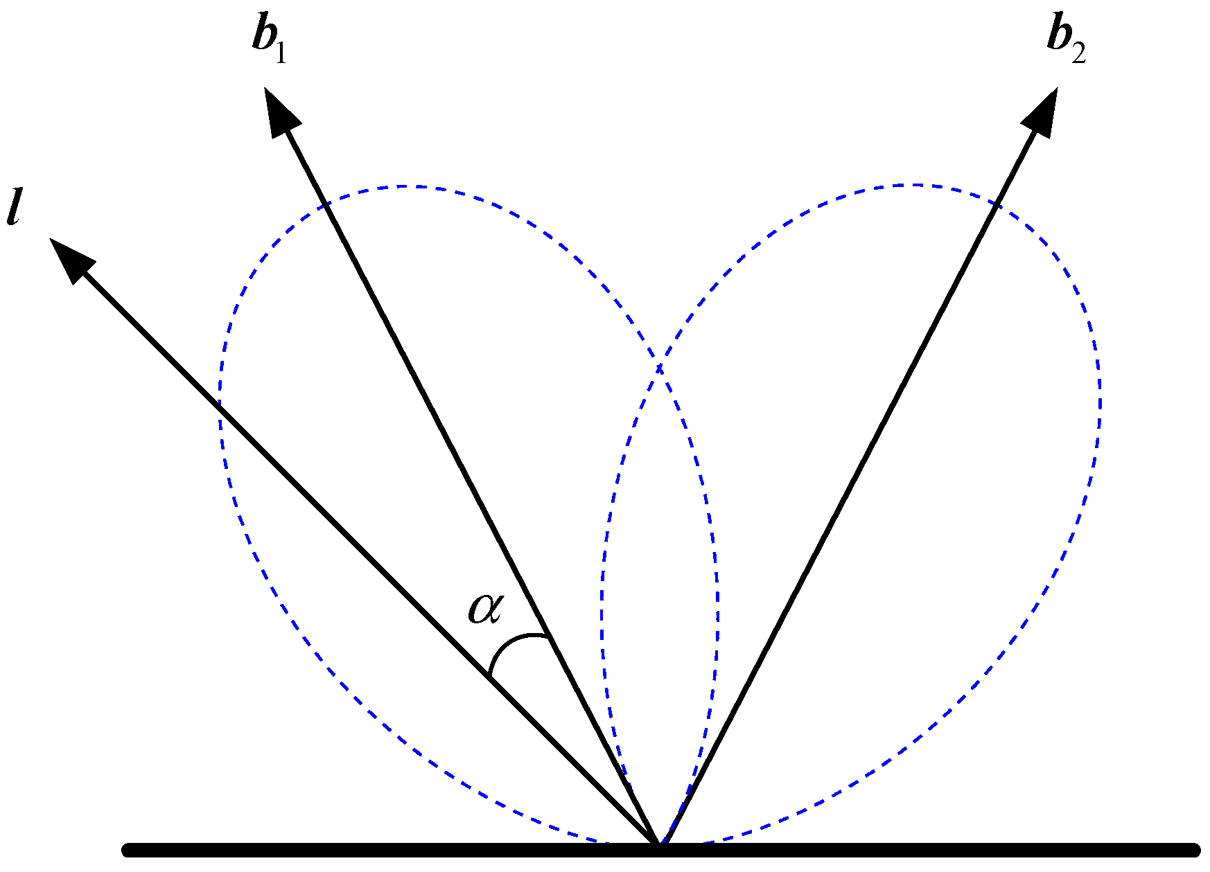
Consider a spaceborne ADS-B receiver connected to two receiving antennas, e.g., helical antennas which have been deployed on GOMX series satellites [17,18]. Figure 1 gives an illustration of antenna configuration. The two antennas have identical gain pattern models and their boresight vectors are represented by two unit vectors, ${\mathit{b}}_1$ and ${\mathit{b}}_2$, respectively. The gain of each antenna has its highest value along the boresight vector and decreases with increasing of the off-boresight angle. The azimuthal variations are small enough to be negligible. Assume that an ADS-B signal transmitted from an aircraft is received by the first antenna. The LOS vector from the satellite to the aircraft can be computed from their known positions and is represented by a unit vector l. Let α denote the off-boresight angle of l with respect to ${\mathit{b}}_1$. As the SNR of the signal is a strictly monotonic function of the off-boresight angle, α can be uniquely determined from the measured value of the SNR. Furthermore, if an ADS-B signal of a second aircraft from a different direction is also received by the same antenna, its boresight vector ${\mathit{b}}_1$ can be estimated from the two derived off-boresight values. This process is called single-axis attitude determination and has been well studied in [16].

Similar to ${\mathit{b}}_1$, the boresight vector ${\mathit{b}}_2$ can also be estimated if the second antenna receives ADS-B signals of two aircraft from different directions. The aircraft and satellite positions are usually expressed in the Earth-centered Earth-fixed (ECEF) frame in consideration that they are derived from GNSS receivers. Accordingly, the estimation of boresight vectors ${\mathit{b}}_1$ and ${\mathit{b}}_2$ refers to the ECEF frame. The estimated coordinates of ${\mathit{b}}_1$ and ${\mathit{b}}_2$ can be further transformed to the satellite’s Vehicle Velocity Local Horizontal (VVLH) frame via orbital information. Finally, since the local coordinates of ${\mathit{b}}_1$ and ${\mathit{b}}_2$ in the satellite’s body frame are known beforehand, the satellite’s three-axis orientation relative to the VVLH frame can be determined.

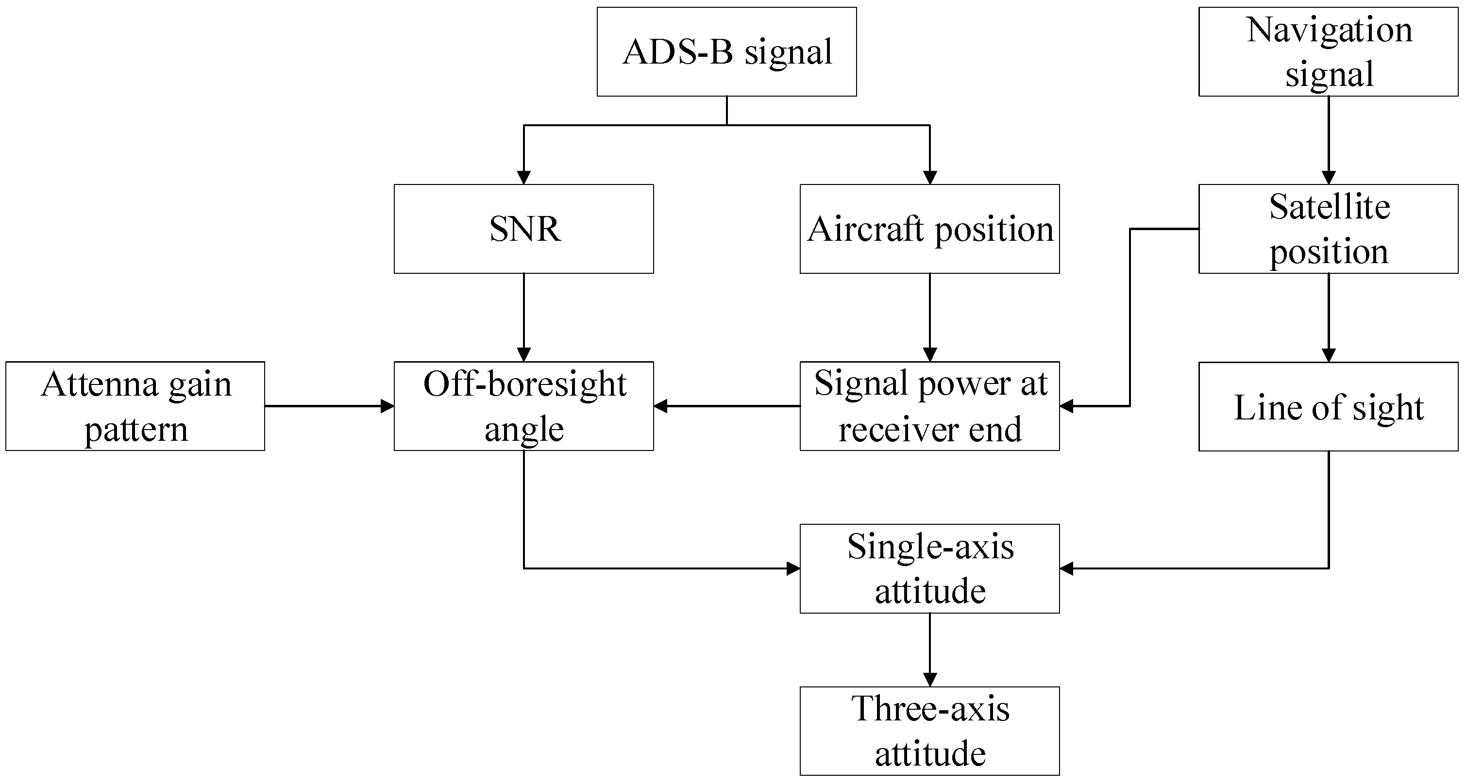
The basic principle of three-axis attitude determination using an ADS-B receiver is summarized in Figure 2. On the one hand, the SNR of the ADS-B signal can be measured. On the other hand, the aircraft identity and position can be decoded from the signal. Then, the off-boresight angle of the signal can be derived from the known calibrated antenna gain pattern. Once off-boresight angles of two or more aircraft are estimated, the antenna boresight vector or the satellite’s single-axis attitude can be obtained. If two or more noncollinear antennas or a multibeam antenna is mounted on the satellite, a complete three-axis attitude determination of the satellite will be viable. It should be noted that the principle of Figure 2 does not mean a completely identical implementation procedure of three-axis attitude determination. As will be shown in the following section, the step of single-axis attitude determination can be entirely skipped.

3. ADS-B-Based Attitude Determination Algorithm

3.1. Attitude Determination Model

The SNR of ADS-B signals is defined as follows:

$$SNR=10\lg \left(\frac{P_s}{P_n}\right)$$

(1)

where $P_s$ and $P_n$ are the signal power and noise power. The noise power is given by [26]:

$$P_n=k_{B}TB$$

(2)

where $k_B$ is the Boltzmann constant (1.381 × 10⁻²³ J/K), B is the measurement bandwidth and T is the effective noise temperature. The signal power is given by the following:

$$P_s=g\left(\alpha \right)P_0$$

(3)

where α is the off-boresight angle, namely, the angle between the boresight vector and the LOS vector from the satellite to aircraft, $g(\cdot )$ is the mapping function of the antenna gain pattern and $P_0$ is the isotropic signal power level at the receiver position.

Principal sources of error of the above observation system include the following: (1) the calculation error of $P_0$ due to estimation errors of the transmitting power and path losses; (2) the modeling error of $g(\cdot )$ due to a calibration error of the antenna gain pattern; and (3) the SNR measurement error induced by the receiver itself. The observation equation considering errors is given as follows:

$$y=10\lg g\left(\alpha \right)+10\lg P_0-10\lg P_n+\nu$$

(4)

where $y$ is the measured value of the SNR and $\nu$ is the total observation error, assumed to be white Gaussian noise in this study. It is noted that α is the only unknown variable in Equation (4).

As it is defined, α is related to the boresight vector and the LOS vector by the following:

$$\cos \alpha =\mathit{l}\cdot \mathit{b}$$

(5)

with b being the boresight vector and l being the LOS vector. b and l are unit vectors. By expressing Equation (5) in the satellite’s body frame, we have the following:

$$\cos \alpha ={\left\{\mathit{l}\right\}}_B^T{\left\{\mathit{b}\right\}}_B$$

(6)

where the subscript ‘B’ denotes the body frame, ${\left\{\mathit{l}\right\}}_B$ and ${\left\{\mathit{b}\right\}}_B$ are coordinates of l and b in the body frame and the superscript ‘T’ denotes the transpose operator.

To determine the attitude of a satellite with the measured value of the SNR, $y$ should be expressed as the function of the attitude explicitly. Thus, $\alpha$ needs to be expressed by the attitude. For a satellite, the attitude is defined as being between the body frame and orbit frame. Equation (6) can be further reformulated as follows:

$$\cos \alpha ={\left({\mathit{C}}_o^B{\left\{\mathit{l}\right\}}_o\right)}^T{\left\{\mathit{b}\right\}}_B$$

(7)

where subscript $o$ denotes the orbit frame.

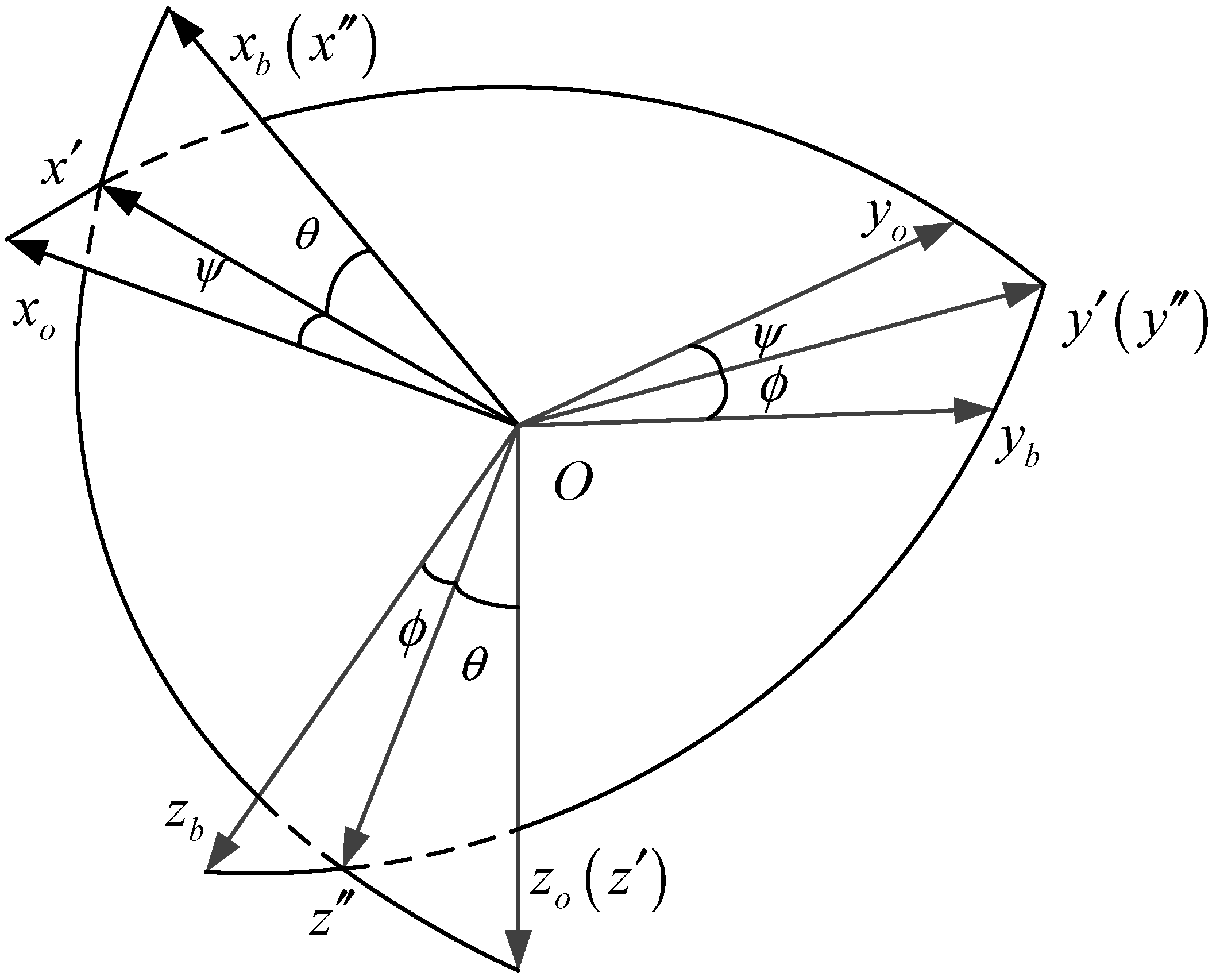
$C_o^B$ is the satellite attitude matrix which needs to be solved. In general, $C_o^B$ can be expressed by three Euler angles. For a 3-2-1 rotation, as is shown in Figure 3, the relationship between the attitude matrix and Euler angle is given by the following:

$$C_o^B=\left[\begin{array}{ccc}\cos \theta \cos \psi & \cos \theta \sin \psi & -\sin \theta \\ \sin \varphi \sin \theta \cos \psi -\cos \varphi \sin \psi & \sin \varphi \sin \theta \sin \psi +\cos \varphi \cos \psi & \sin \varphi \cos \theta \\ \cos \varphi \sin \theta \cos \psi +\sin \varphi \sin \psi & \cos \varphi \sin \theta \sin \psi -\sin \varphi \cos \psi & \cos \varphi \cos \theta \end{array}\right]$$

(8)

where $\psi$, $\theta$ and $\varphi$ are the yaw, pitch and roll angles, respectively.

${\left\{l\right\}}_o$ is the unit line of the sight vector expressed in the orbit coordinate frame; it can be calculated by the following:

$${\left\{l\right\}}_o=\frac{x_o^s-x_o^a}{\Vert x_o^s-x_o^a\Vert }$$

(9)

where $x_o^s$ and $x_o^a$ denote the satellite position and aircraft position expressed in the orbit frame of the satellite, respectively.

${\left\{b\right\}}_B$ is the unit boresight vector expressed in the satellite body frame. It is determined by the antenna mounting position.

By substituting these equations into Equation (1), it is possible to relate the SNR measurement value $y$ and satellite attitude $C_o^B$:

$$y=10\lg g\left(\arccos \left({\left(C_o^b\frac{x_o^s-x_o^a}{\Vert x_o^s-x_o^a\Vert }\right)}^T{\left\{b\right\}}_B\right)\right)+\epsilon$$

(10)

where

$$\epsilon =10\lg P_0-10\lg P_n+\nu$$

(11)

From the signals received from different aircraft, $x_o^s$, ${\left\{l\right\}}_o$ and ${\left\{b\right\}}_B$ are known; the SNR measurement only is a function of the satellite attitude $C_o^b$ and aircraft position $x_o^a$. Meanwhile, $C_o^b$ can be expressed by three Euler angles, $\psi$, $\theta$ and $\varphi$, in order to avoid orthogonality for the attitude matrix. Above all, the observation equation can be written as follows:

$$y=f\left(x_o^a,\psi ,\theta ,\varphi \right)+\epsilon$$

(12)

where

$$f\left(x_o^a,\psi ,\theta ,\varphi \right)=10\lg g\left(\arccos \left({\left(C_o^b\frac{x_o^s-x_o^a}{\Vert x_o^s-x_o^a\Vert }\right)}^T{\left\{b\right\}}_B\right)\right)$$

(13)

In order to keep the notation as compact as possible, let $x$ denote the aircraft position $x_o^a$; then, the observation equation can be rewritten as follows:

$$y=f\left(x,\psi ,\theta ,\varphi \right)+\epsilon$$

(14)

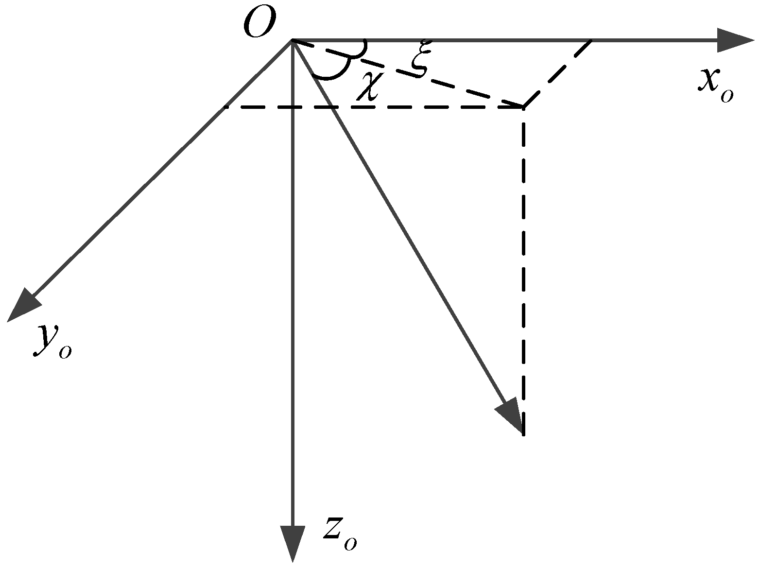
As is discussed in the previous section, rotations on the boresight orientation are unavailable because of the symmetry of the antenna gain pattern. The single-axis attitude is estimated when one antenna is mounted on the spacecraft. Equation (14) can be rewritten as follows:

$$y=f_1\left(x,\xi ,\chi \right)+\epsilon$$

(15)

where $\xi$ and $\chi$ are the azimuth angle and elevation angle of the boresight vector expressed in the orbit frame, as is shown in Figure 4. This case has been discussed by Kaixing Zhou and Xiucong Sun et al. For more details, see [16].

3.2. Attitude Determination by Deterministic Method

In this section, we will discuss how to estimate satellite three-axis attitude using two or more ADS-B antennas. A class of solution for this problem is known as the deterministic method. They can estimate satellite attitude directly using two or more observation vectors.

The basic idea for the deterministic method can be expressed by the following:

$${\left\{b_i\right\}}_B=C_o^b{\left\{b_i\right\}}_o+{\varsigma }_i\hspace{1em}\hspace{1em}\hspace{1em}\hspace{1em}\hspace{1em}\hspace{1em}\hspace{1em}i=1,2,\cdots n$$

(16)

where ${\left\{b_i\right\}}_B$ and ${\left\{b_i\right\}}_o$ denote the i-th boresight vector expressed in the body frame and orbit frame, respectively, and ${\varsigma }_i$ is the corresponding error. In Equation (16), $({\left\{b_i\right\}}_B,{\left\{b_i\right\}}_o)$ is a set of observation vectors, which contain the information on the attitude. Wahba [27] described the problem of finding the attitude matrix as the orthogonal matrix that minimizes the loss function; this question is known as Wahba’s Problem:

$$L\left(C_o^b\right)=\frac{1}{2}{\displaystyle \sum _{i=1}^n{a}_i}{\Vert {\left\{b_i\right\}}_B-C_o^b{\left\{b_i\right\}}_B\Vert }^2$$

(17)

where $a_i$ denotes the i-th non-negative weight.

Achievements have been made by researchers in recent years. A lot of algorithms have been proposed to solve the question, for example, the three-axis attitude determination algorithm (TRIAD) [28], Davenport’s q method [29], the Quaternion estimator (QUEST) [30], the Singular Value Decomposition method (SVD) [31], the Fast optimal attitude matrix (FOAM) [32] and so on. Among them, QUEST is the most commonly used attitude determination algorithm due to its higher precision and faster operational speed relative to the other methods. For more detail about QUEST, see [30].

Above all, the process of ADS-B-based three-axis attitude determination using a deterministic method can be divided into two steps:

1.

Estimating a set of observation vectors $({\left\{b_i\right\}}_B,{\left\{b_i\right\}}_o)$. The former can be obtained by the antenna mounting position direction, while the latter can be determined by Equation (15).

2.

Determining the satellite attitude using the QUEST algorithm.

3.3. Attitude Determination by Nonlinear Least Squares Estimation (NLSE)

ADS-B-based three-axis attitude determination using a deterministic method has been discussed in the previous section. However, the method might lead to a larger error, because the estimation process is divided into two steps with an estimation error. Therefore, it is necessary to estimate the satellite three-axis attitude in one step for a more precise attitude determination.

Assuming that there are $n$$\left(n\ge 2\right)$ antennas deployed on the satellite, and letting $m_i$ $(m_i\ge 3,0\le i\le n)$ be the number of available aircraft for the i-th antenna, for the i-th antenna, the measured value of the SNR related to the j-th $(0\le j\le m_i)$ aircraft is given as follows:

$$y_{ij}=f_i\left(x_j,\psi ,\theta ,\varphi \right)+{\epsilon }_{ij}$$

(18)

where $x_j$ denotes the position of the j-th available aircraft, and $f_i\left(x_j,\psi ,\theta ,\varphi \right)$ and ${\epsilon }_{ij}$ denote the values of Equations (13) and (11) for the i-th antenna and j-th aircraft, respectively.

Since $f\left(x,\psi ,\theta ,\varphi \right)$ is a nonlinear function, the satellite three-axis attitude determination is virtually a nonlinear least squares (NLS) problem. The objective function for this problem is as follows:

$$F\left(z\right)=\frac{1}{2}{\displaystyle \sum _{i=1}^n{\displaystyle \sum _{j=1}^{m_i}{\left\{y_{ij}-f_i\left(x_j,z\right)\right\}}^2}}$$

(19)

where $z={[\psi ,\theta ,\varphi ]}^T$.

Satellite three-axis attitude determination is equivalent to the following minimization problem:

$$z_{opt}=argmin\left\{F\left(z\right)\right\}$$

(20)

where $argmin\left\{F\left(z\right)\right\}$ denotes the point $z$ at which $F\left(z\right)$ achieves the minimum value.

There have been a lot of studies for the nonlinear least squares problem [33,34,35]. The most commonly employed nonlinear least squares estimation method is the numerical iteration method, including the levenberg–marquardt algorithm (LMA or LM) [33], the Gauss–Newton algorithm [34] and the gradient descent algorithm [35].

The Gauss–Newton algorithm has a fast convergence, but it needs to calculate the Jacobian matrix of the objective function, and also requires the matrix to be positively determined. When the matrix is almost singular, the algorithm will produce an ill-fitting phenomenon. Although the gradient descent algorithm has a global convergence, it converges too slowly.

The levenberg–marquardt algorithm, also known as the damped least-squares (DLS) method, is proposed to overcome the issue that the iterative matrix is ill-conditioned in the Gauss–Newton algorithm. The levenberg–marquardt algorithm interpolates between the Gauss–Newton algorithm and the method of gradient descent. The levenberg–marquardt algorithm is more robust than the Gauss–Newton algorithm, which means that it finds a solution even if it starts very far off the final minimum in many cases.

The key for the levenberg–marquardt algorithm is solving the following equation:

$$\left(J^{T}J+\lambda I\right)\delta =J^T\left(y-f\left(x,z\right)\right)$$

(21)

where $J$ is the Jacobian matrix, $\lambda$ is the damping factor, $I$ is the identity matrix and $\delta$ is the increment for the initial estimated parameter value $z_0$. $y$ and $f\left(x,z\right)$ are stacked vectors of $y_{ij}$ and $f_i\left(x_j,z\right)$, respectively.

The damping factor $\lambda$ is non-negative and is adjusted at each iteration. If the reduction of $F\left(z\right)$ is rapid, a smaller value can be used, bringing the algorithm closer to the Gauss–Newton algorithm, whereas if an iteration gives insufficient reduction in the residual, $\lambda$ can be increased, moving a step closer to the gradient-descent direction. If either the length of the calculated step $\delta$ or the reduction of the objective function $F\left(z\right)$ fall below predefined limits, iteration stops and the last parameter vector $z$ is considered to be the solution.

The variance–covariance matrix for the attitude estimation error can be obtained by Equation (22):

$$R={\left(J^{T}CJ\right)}^{-1}$$

(22)

where $C=diag\left(\frac{1}{{\sigma }_{11}^2},\cdots ,\frac{1}{{\sigma }_{1m_1}^2},\frac{1}{{\sigma }_{21}^2},\cdots ,\frac{1}{{\sigma }_{ij}^2},\cdots \frac{1}{{\sigma }_{n{m}_n}^2}\right)$, and ${\sigma }_{ij}$ is the standard deviation of the corresponding SNR measurement $y_{ij}$.

4. Multiplicative Extended Kalman Filter (MEKF) for ADS-B/Gyro Attitude Determination

In the previous section, a new satellite three-axis attitude determination method based on two or more noncollinear ADS-B-receiving antennas was proposed. Despite the lower cost compared with the typical solutions, the accuracy of the ADS-B-based solution is rough (approximately in degree-level). Moreover, the ADS-B-based solution is available only when the number of observations for each antenna is no less than three, which makes it difficult to provide a long-term attitude determination. To achieve a higher accuracy and more robust attitude determination, it is imperative to combine the ADS-B signal observations with other attitude determination sensors.

4.1. Gyro Model

Gyro is a typical attitude sensor. The measured output of the gyro is the satellite three-axis angular rate relative to the inertial reference frame. The dynamics performance of the attitude is included in the gyro measurement, which is helpful to improve the attitude determination accuracy. For a rate-integrating gyro, a widely used model is given by Equations (23) and (24):

$${\tilde{\mathsf{\omega }}}_b={\mathsf{\omega }}_b+\mathsf{\beta }+{\mathsf{\eta }}_v$$

(23)

$$\dot{\mathsf{\beta }}={\mathsf{\eta }}_u$$

(24)

where ${\tilde{\mathsf{\omega }}}_b$ is the measured angular rate, ${\mathsf{\omega }}_b$ is the true angular rate and subscript $b$ means the body frame. $\mathsf{\beta }$ denotes the gyro drift, which is assumed to be governed by (24). ${\mathsf{\eta }}_v$ and ${\mathsf{\eta }}_u$ are independent zero-mean Gaussian white noise processes with the following:

$$\begin{array}{l}E\left\{{\eta }_v\left(t\right){\eta }_v^T\left(\tau \right)\right\}={\sigma }_v^2\delta \left(t-\tau \right)I_{3\times 3}\\ E\left\{{\eta }_u\left(t\right){\eta }_u^T\left(\tau \right)\right\}={\sigma }_u^2\delta \left(t-\tau \right)I_{3\times 3}\end{array}$$

(25)

where $E\{•\}$ denotes expectation and $\delta \left(t-\tau \right)$ is the Dirac delta function.

4.2. Attitude Error Vector

In this section, the measurement data of the ADS-B and gyro are fused by multiplicative extended Kalman filter (MEKF). MEKF was first developed in 1969 by Toda, Heiss et al. It has been used for attitude estimation of several onboard NASA spacecraft. The MEKF describes the attitude as the product of an estimated attitude and an attitude error from that estimate attitude, as is shown in the following:

$$q=\delta q\left(\upsilon \right)\otimes \widehat{q}$$

(26)

where $q$ is the unit true attitude quaternion, $\widehat{q}$ is the unit estimated attitude quaternion and $\delta q\left(\upsilon \right)$ is a unit error quaternion representing the rotation from $\widehat{q}$ to $q$, which is parameterized by a three-component vector $\upsilon$, called the attitude error vector. $\upsilon$ can be described in different ways, including as two times the vector part of the quaternion, two times the vector of Rodrigues or Gibbs, four times the vector of modified Rodrigues parameters (MPRs) or integrated rate parameters, the vector of infinitesimal rotation angles and so on. These definitions of $\upsilon$ are equivalent for EKF, because they have the same first-order approximation:

$$\delta q\left(\upsilon \right)\approx \left[\begin{array}{c}\frac{\upsilon }{2}\\ 1\end{array}\right]$$

(27)

In these contributions, we use four times the vector of MPRs to describe the attitude error vector, giving the following:

$$\delta q\left(\upsilon \right)\approx \frac{1}{16+{\Vert \upsilon \Vert }^2}\left[\begin{array}{c}8\upsilon \\ 16-{\Vert \upsilon \Vert }^2\end{array}\right]$$

(28)

For the MEKF process, the attitude error vector is treated as a part of the state vector. The dynamics equation of the attitude error vector is given by the following:

$$\dot{\upsilon }=-{\omega }_b\times \upsilon +∆\omega$$

(29)

where $∆\omega$ is the error of the angular rate with the following:

$$∆\omega ={\omega }_b-{\widehat{\omega }}_b$$

(30)

4.3. State Model

For the attitude determination by measurements from the ADS-B receivers and gyro, the state vector is chosen as follows:

$$X=\left[\begin{array}{c}\upsilon \\ ∆\mathsf{\beta }\end{array}\right]$$

(31)

where $∆\mathsf{\beta }$ denotes the error of the gyro drift, defined as follows:

$$∆\mathsf{\beta }=\mathsf{\beta }-\widehat{\mathsf{\beta }}$$

(32)

with $\widehat{\mathsf{\beta }}$ being the estimated gyro drift, according to the gyro model in Equation (23):

$${\tilde{\mathsf{\omega }}}_b={\widehat{\mathsf{\omega }}}_b+\widehat{\mathsf{\beta }}$$

(33)

$$∆\dot{\mathsf{\beta }}={\mathsf{\eta }}_u$$

(34)

By substituting Equations (23) and (32) into (33), it is possible to relate the $∆\mathsf{\omega }$ and $∆\mathsf{\beta }$:

$$∆{\mathsf{\omega }}_b=-∆\mathsf{\beta }-{\mathsf{\eta }}_v$$

(35)

Dynamics equations of the attitude error vector can be reformulated as follows:

$$\dot{\mathsf{\upsilon }}=-{\mathsf{\omega }}_b\times \mathsf{\upsilon }-∆\mathsf{\beta }-{\mathsf{\eta }}_v$$

(36)

According to Equations (34) and (36), the state model of the state vector $X$ is given by the following:

$$\dot{X} = AX + W$$

(37)

where $A$ is the state transition matrix and $W$ is the process noise; they are expressed as follows:

$$A=\left(\begin{array}{cc}-\left[{\widehat{\omega }}_b\times \right]& I_{3\times 3}\\ 0_{3\times 3}& 0_{3\times 3}\end{array}\right)$$

(38)

$$W=\left(\begin{array}{c}-{\mathsf{\eta }}_v\\ {\mathsf{\eta }}_u\end{array}\right)$$

(39)

with $I_{3\times 3}$ as the identity matrix, $0_{3\times 3}$ as the zeros matrix and $\left[{\widehat{\omega }}_b\times \right]$ as the cross matrix of $\widehat{\mathsf{\omega }}$.

The variance–covariance matrix of $W$ is written as follows:

$$Q=\left(\begin{array}{cc}{\sigma }_v^2{I}_{3\times 3}& 0_{3\times 3}\\ 0_{3\times 3}& {\sigma }_u^2{I}_{3\times 3}\end{array}\right)$$

(40)

4.4. Observation Model

In Section 3, we discussed how to estimate the satellite three-axis attitude by using ADS-B measurement, using the Euler angle (3-2-1 rotation) to express attitude. In this section, the Euler angle errors ${[∆\psi ,∆\theta ,∆\varphi ]}^T$ are chosen as the measurement of MEKF, as follows:

$$Z=\left(\begin{array}{c}∆\psi \\ ∆\theta \\ ∆\varphi \end{array}\right)=\left(\begin{array}{c}\tilde{\psi }\\ \tilde{\theta }\\ \tilde{\varphi }\end{array}\right)-\left(\begin{array}{c}\widehat{\psi }\\ \widehat{\theta }\\ \tilde{\varphi }\end{array}\right)$$

(41)

where $Z$ denotes the observation of MEKF, ${\left[\tilde{\psi },\tilde{\theta },\tilde{\varphi }\right]}^T$ is the attitude angle calculated using ADS-B observations and ${\left[\widehat{\psi },\widehat{\theta },\widehat{\varphi }\right]}^T$ is the attitude angle estimated using the state model.

According to [36], the differential kinematic equations relate the (3-2-1) Euler angle rates to the angular velocity vector through the following:

$$\left(\begin{array}{c}\dot{\psi }\\ \dot{\theta }\\ \dot{\varphi }\end{array}\right)=\left(\begin{array}{ccc}0& \frac{\sin \varphi }{\cos \theta }& \frac{\cos \varphi }{\cos \theta }\\ 0& \cos \varphi & -\sin \varphi \\ 1& \tan \theta \sin \varphi & \tan \theta \cos \varphi \end{array}\right)\left(\begin{array}{c}{\omega }_x\\ {\omega }_y\\ {\omega }_z\end{array}\right)$$

(42)

From the view of the change rate, and by applying the small-angle approximation to Equation (42), we can relate observation $Z$ to attitude error vector $\upsilon$ as follows:

$$Z=H_{\upsilon }\upsilon$$

(43)

with

$$H_{\upsilon }=\left(\begin{array}{ccc}0& \frac{\sin \widehat{\varphi }}{\cos \widehat{\theta }}& \frac{\cos \widehat{\varphi }}{\cos \widehat{\theta }}\\ 0& \cos \widehat{\varphi }& -\sin \widehat{\varphi }\\ 1& \tan \widehat{\theta }\sin \widehat{\varphi }& \tan \widehat{\theta }\cos \widehat{\varphi }\end{array}\right)$$

(44)

Finally, the observation model is written as follows:

$$Z=HX+V$$

(45)

where $H$ is the observation matrix, as shown below:

$$H=\left[\begin{array}{cc}{H}_{\upsilon }& 0_{3\times 3}\end{array}\right]$$

(46)

$V$ is the observation noise, which is zero-mean Gaussian white noise, and its covariance matrix is $R$.

4.5. Filtering and Update

• Discretization

Before filtering and updating, a discretization step needs to be done because the state model is represented as a continuous time model, while discrete time measurements are frequently taken for state estimation via the ADS-B receiver and gyro. A simple discretization method is as follows [37]:

$$F_{k/k-1}=I+T{A}_{k-1}+\frac{T^2}{2!}{A}_{k-1}^2+\frac{T^3}{3!}{A}_{k-1}^3+\cdots$$

(47)

where $F_{k/k-1}$ is the discrete state transition matrix, $A_{k-1}$ is the continuous state transition matrix and $T$ is the sample period. Applying the discretization method to our work, the discrete state mode and observation mode are obtained as follows:

$$X_k=F_{k/k-1}{X}_{k-1}+W_k$$

(48)

$$Z_k=H_k{X}_k+V_k$$

(49)

$$W_k\sim N\left(0,Q_k\right),V_k\sim N\left(0,R_k\right)$$

(50)

2.

Time update

Once we obtain the discrete state mode and observation mode, the filtering and updating process can be performed. An a priori estimate of the state vector at epoch $t_k$ can be obtained from the following steps:

$$X_{k/k-1}=F_{k,k-1}{X}_{k-1}$$

(51)

$$P_{k/k-1}=F_{k/k-1}{P}_{k-1}{F}_{{}_{k/k-1}}^T+Q_{k-1}$$

(52)

where $X_{k/k-1}$, $P_{k/k-1}$ is the a priori estimate of the state vector and its error covariance matrix:

$$X_{k/k-1}=\left[\begin{array}{c}{\widehat{x}}_{k/k-1}\\ ∆{\widehat{\mathsf{\beta }}}_{k/k-1}\end{array}\right]$$

(53)

$$P_{k/k-1}=\left[\begin{array}{cc}{P}_{{\widehat{\upsilon }}_{k/k-1}}& \\ & P_{∆{\widehat{\mathsf{\beta }}}_{k/k-1}}\end{array}\right]$$

(54)

The a priori estimation of attitude quaternion ${\widehat{q}}_k$ is obtained by the following:

$${\widehat{q}}_k=\delta q\left({\widehat{\upsilon }}_{k/k-1}\right)\otimes q_{k-1}$$

(55)

while the a priori estimation of the attitude angle ${\left[\widehat{\psi },\widehat{\theta },\widehat{\varphi }\right]}^T$ can be given from ${\widehat{q}}_k$.

3.

Measurement update

In the measurement update phase, the filter updates the estimate of the state vector and its covariance matrix as follows:

$$X_k=X_{k/k-1}+K_k\left(Z_k-H_k{X}_{k/k-1}\right)$$

(56)

$$P_k=\left(I-K_k{H}_k\right)P_{k/k-1}$$

(57)

with $K_k$ as the filter gain:

$$K_k=P_{k/k-1}{H}_k^T{\left(H_k^{}{P}_{k/k-1}{H}_k^T+R_k\right)}^{-1}$$

(58)

An important question is how to modify the attitude using the state vector $X_k={\left[\begin{array}{cc}{\upsilon }_k& ∆{\mathsf{\beta }}_k\end{array}\right]}^T$. The error of gyro drift $∆{\mathsf{\beta }}_k$ is used to modify gyro drift $\mathsf{\beta }$ and angular rate ${\omega }_k$:

$${\mathsf{\beta }}_k={\mathsf{\beta }}_{k-1}+∆{\mathsf{\beta }}_{k-1}$$

(59)

$${\mathsf{\omega }}_k={\tilde{\mathsf{\omega }}}_k-{\mathsf{\beta }}_k$$

(60)

while attitude error vector $x_k$ is used to correct the attitude. The corrected attitude quaternion $q_k$ can be obtained by the following:

$$q_k=\delta q\left({\upsilon }_k\right)\otimes {\widehat{q}}_k$$

(61)

while the attitude angle ${\left[\psi ,\theta ,\varphi \right]}^T$ can be given from $q_k$. What should be paid attention to is the fact that the filter needs to be reset when a filtering and updating process is complete, because the error described by the state vector has been corrected after Equations (59) and (61). The reset step is as follows:

$$X_{k-1}={\left[\begin{array}{cccccc}0& 0& 0& 0& 0& 0\end{array}\right]}^T$$

(62)

5. Simulation Results and Analysis

5.1. Simulation Condition

To verify the method proposed to estimate the satellite three-axis attitude based on the ADS-B receiver, a simulation was carried out.

In order to make the simulation result much more accurate and closer to the practical implementation scenario, we apply the actual global flight data of the aircraft to the simulation. The flight data are from the VariFlight, which is a flight service company in China. We utilize the data to find out which aircraft are available, by which we mean that the aircraft are in sight of the space-based ADS-B receiver antenna and the SNR measurements value contained within the ADS-B signal is not less than the system-required SNR ($P_{SNR}^{req}$; $P_{SNR}^{req}=6dB$ in our work).

The simulation is based on the BUAA-Sat microsatellite, which is planned to be launched into a Sun-synchronous orbit, with 600km altitude and 97.8 degree inclination [38], and the satellite is assumed to be at the ideal Earth-pointing attitude in the simulation.

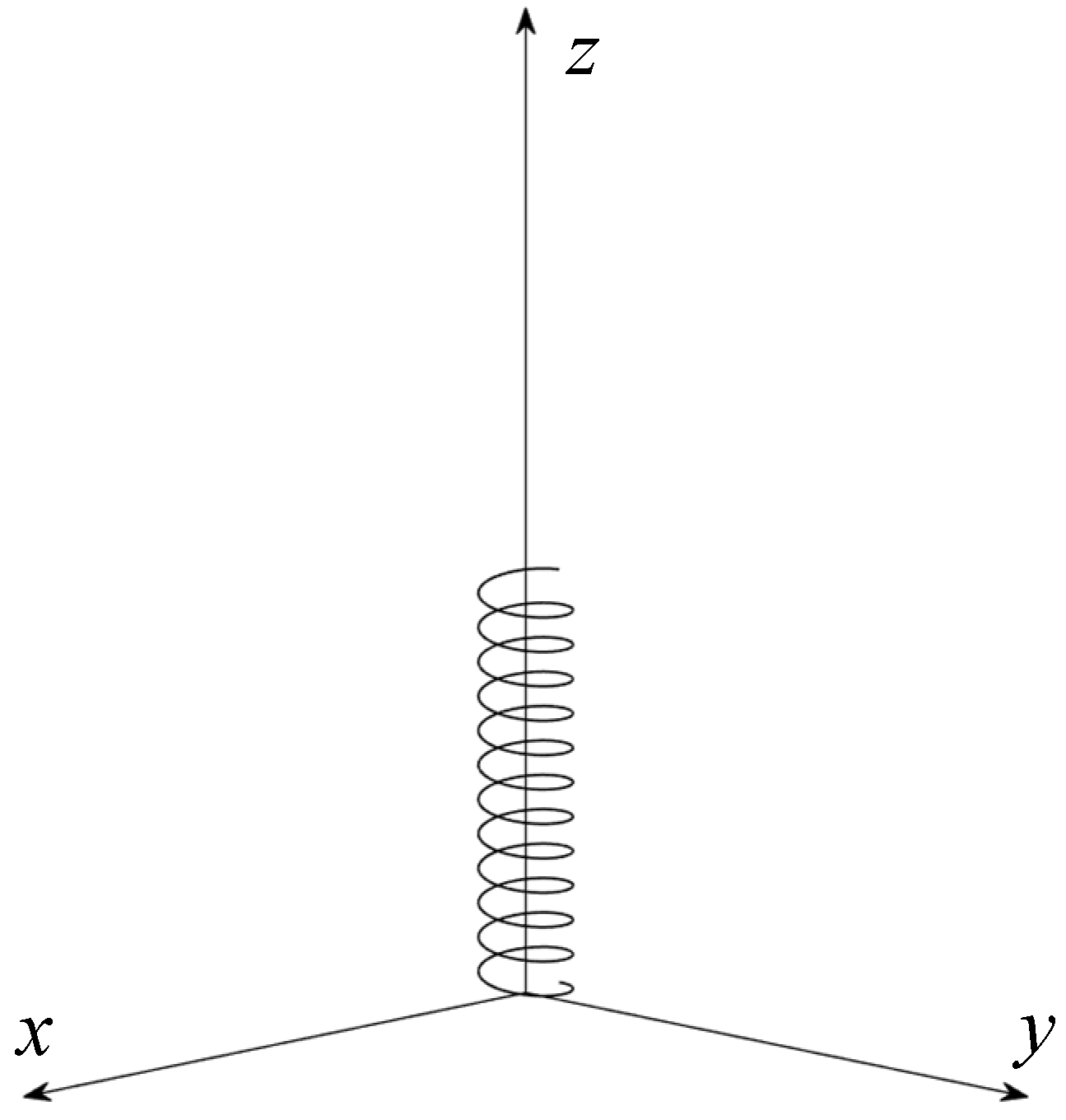
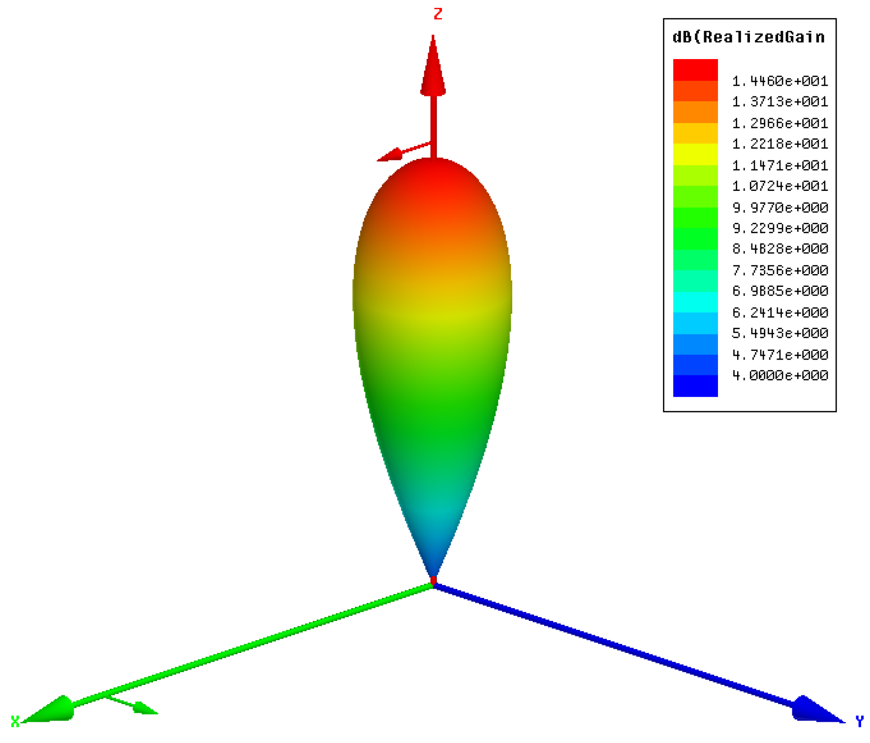
The satellite will equip an ADS-B receiver as one of its payload and a helical antenna is used for receiving the ADS-B signal from the aircraft. The helical antenna is illustrated in Figure 5. As mentioned in Section 2, an important characteristic about the helical antenna is its antenna gain pattern. To find the antenna gain pattern of the helical antenna, we conduct an electromagnetic simulation using a High Frequency Structure Simulator (HFSS). The parameters used for the electromagnetic simulation are shown in

Table 1. The parameter of helical antenna.

Helical Radius (mm)	Pitch (mm)	Wire Diameter (mm)	Twist Number
47	65	2	15

and the result is presented in Figure 6.

Figure 6 only shows the major lobe ($G_{RA}\ge 4dBi$) of the helical antenna gain pattern. From the picture, we can see the antenna gain has a strong directivity along the boresight, which leads to the SNR measurement varying with off-boresight angles as is described in Equation (1). The electromagnetic simulation gives $g\left(\alpha \right)$ mathematical expression:

$$g\left(\alpha \right)=14.4598{\cos }^6\alpha$$

(63)

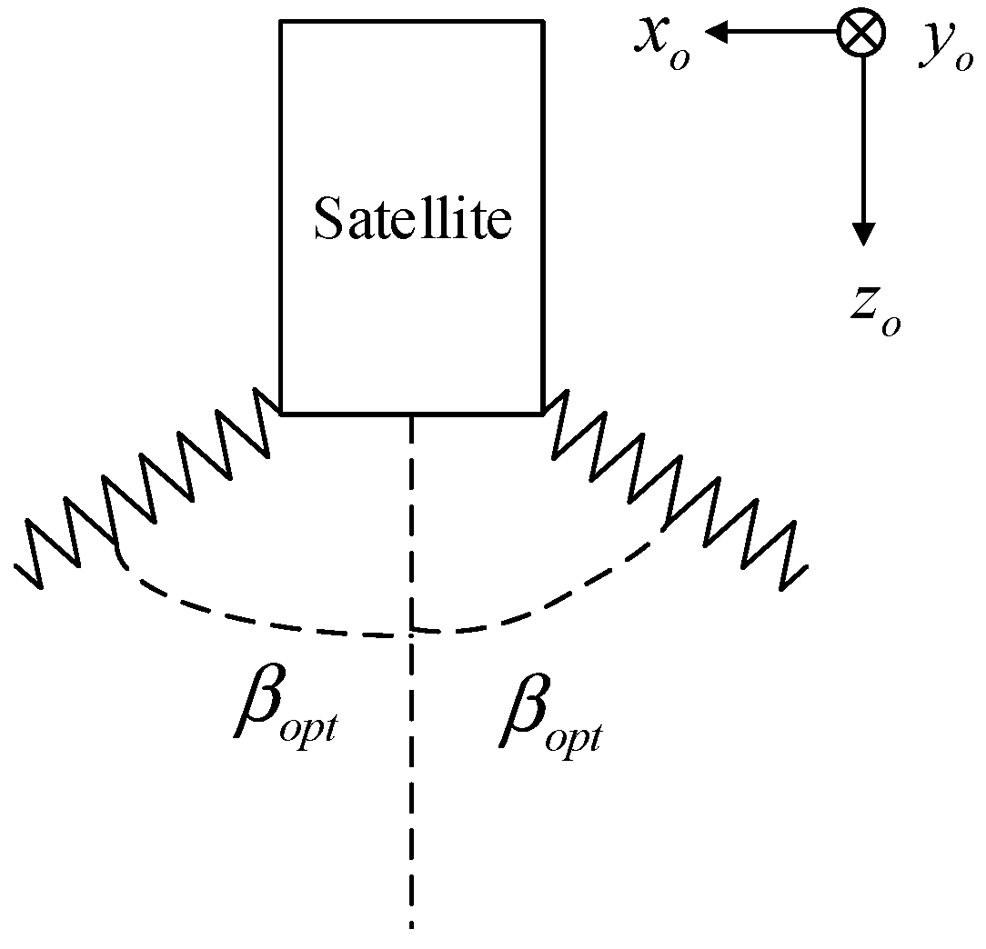
What is more notable about the antenna is its mounting direction. The problem has been solved by Kaixing Zhou and Xiucong Sun et al. [16]. The optimal mounting angle is given as follows:

$${\beta }_{opt}=50.77°$$

(64)

In order to estimate the satellite three-axis attitude, two helical antennas are mounted at the bottom of the satellite, both with the optimal angle. The installation location and geometry configuration of two helical antennas are presented in Figure 7.

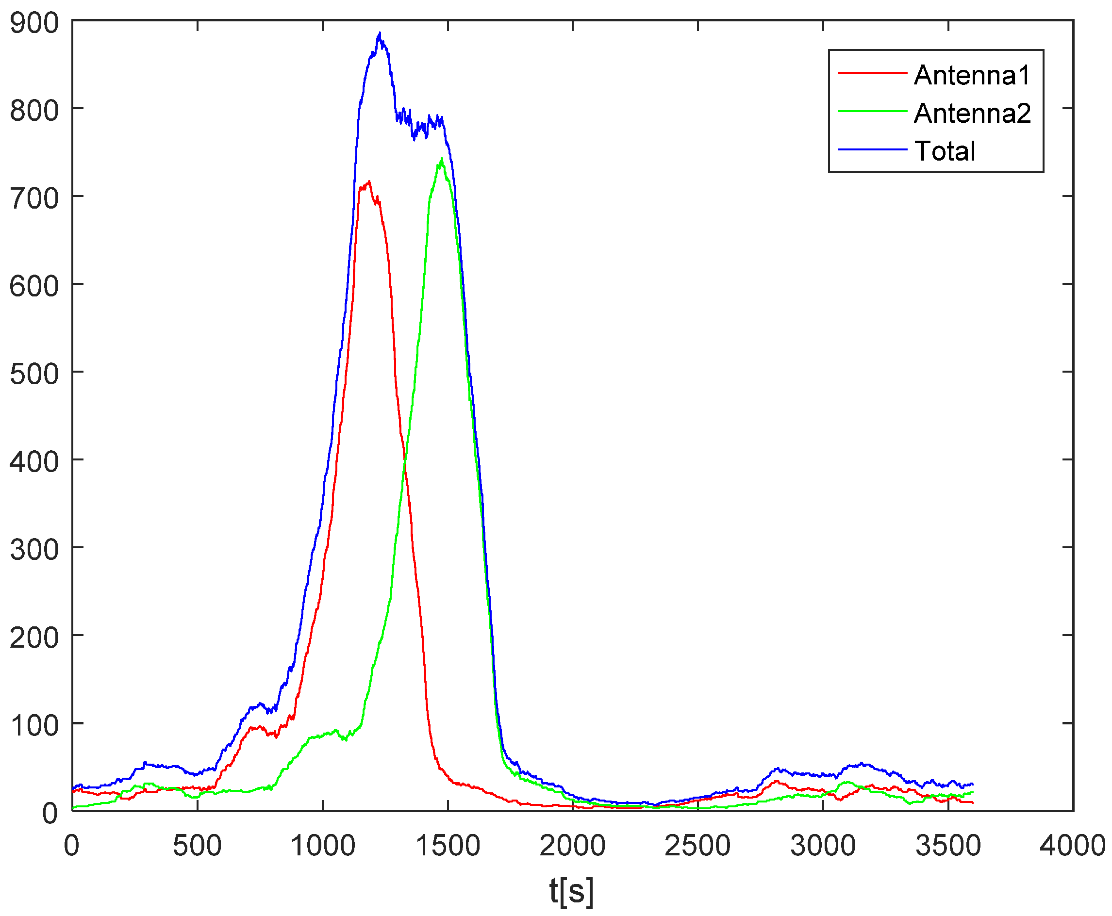
In this work, we use a rate-integrating gyro for MEKF. The parameters of the gyro noise are set as ${\sigma }_v=0.05°/\mathrm{s}$, ${\sigma }_u=0.05°/\mathrm{s}$. The observation noise of the SNR measurement $V$ has standard deviation ${[1dB,1dB,1dB]}^T$, and its covariance matrix is $R={(1dB)}^2\cdot I_{3\times 3}$. An hour of data is chosen for the result analysis; the number of available aircraft for two antennas is not less than three in each time step, as is shown in Figure 8. The number of available aircraft for Antenna1 is shown in red and for Antenna2 is shown in green, while the total available observation (antenna1 + antenna2) is shown in blue.

In the simulation, three ADS-B-based methods proposed in the previous sections are employed to estimate the satellite three-axis attitude; they are the deterministic method, nonlinear least squares estimation (NLSE) method and multiplicative extended Kalman filter (MEKF). The Quaternion estimator (QUES) is used for the deterministic method.

5.2. Result Analysis

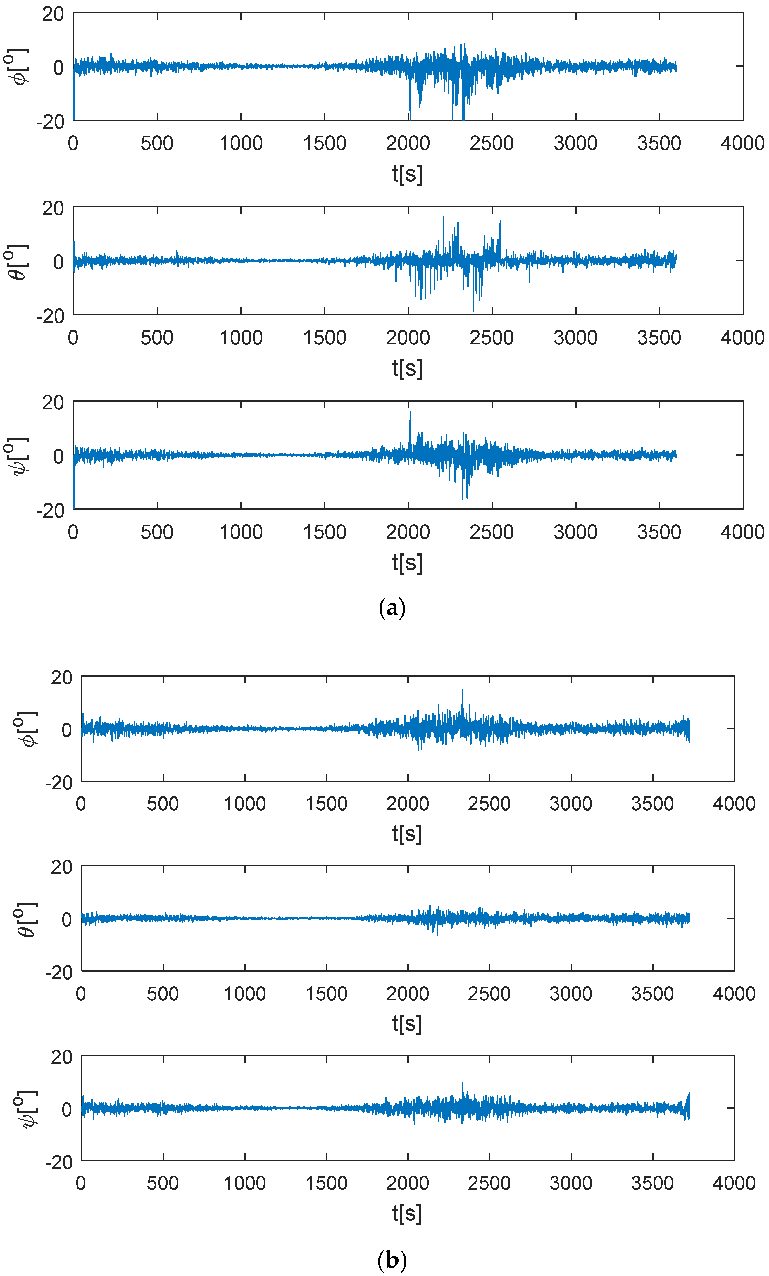
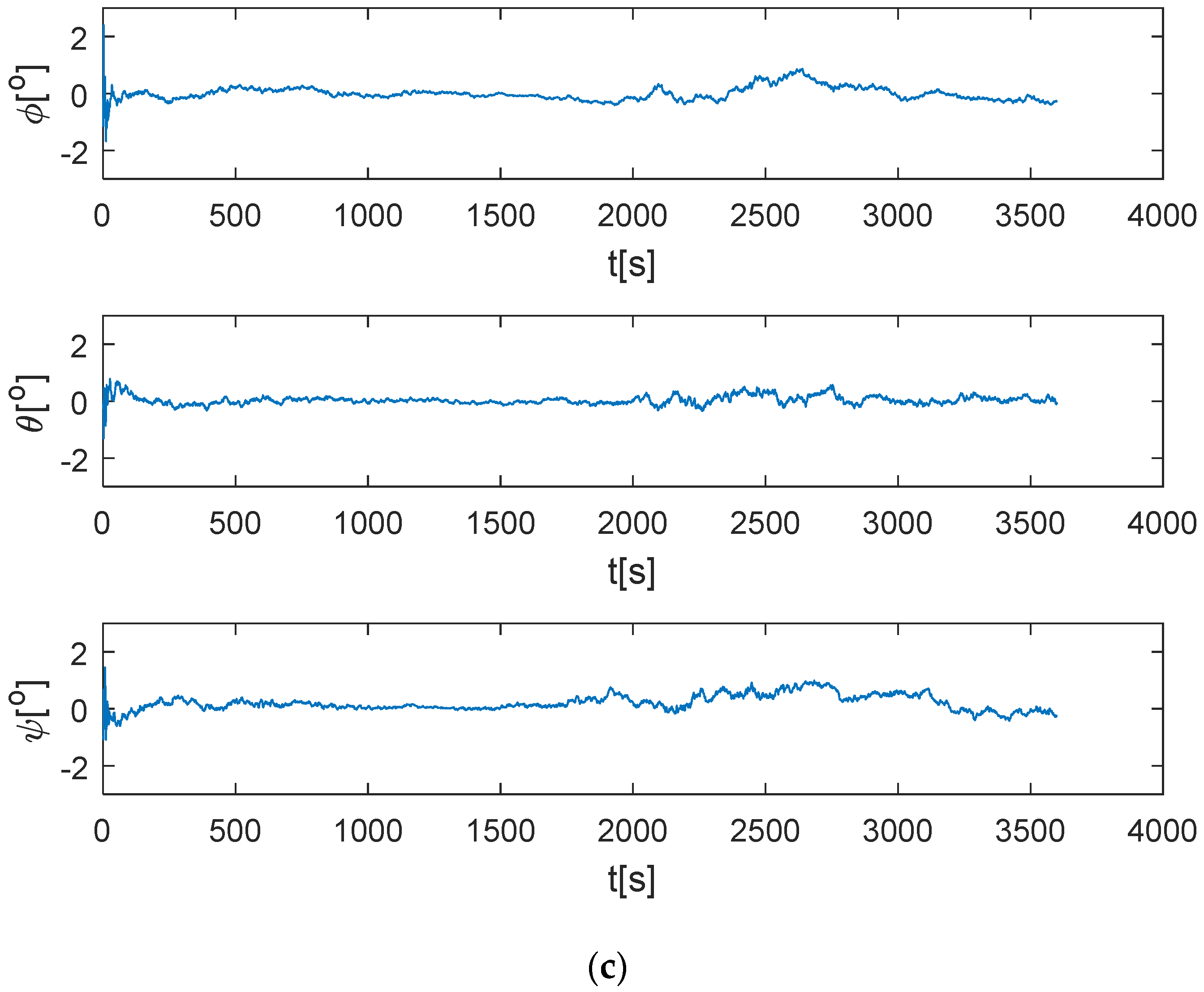
The top panel of Figure 9 shows the estimation error of the Euler angle using the deterministic (QUEST) method in the setting simulation condition. As can be seen in this figure, the attitude estimated using the QUEST method has rough accuracy: the maximum estimation error is more than $\pm 20°$. The middle pane of Figure 9 shows the estimation error using the NLSE method; the three-axis attitude error of NLSE is less than the error estimated using the QUEST method. The maximum estimation error is about $\pm 15°$ for NLSE, while more than $\pm 20°$ for QUEST. The conclusion proves the point proposed in Section 3.3. To further improve the accuracy of attitude determination, the MEKF has been implemented successfully for satellite three-axis attitude determination. From the bottom panel of Figure 9, it can be seen that the attitude determination accuracy of MEKF has an obvious improvement compared with the QUEST method and NLSE method. The estimation error is less than $\pm 3°$.

The statistics of all simulation results are presented in

Table 2. The statistics of all simulation results.

	$\mathbf{Maximum} [°]$			$\mathbf{Root} \mathbf{Mean} \mathbf{Square} [°]$			Running Time [s]
	$\mathit{\psi }$	$\mathit{\theta }$	$\mathit{\varphi }$	$\mathit{\psi }$	$\mathit{\theta }$	$\mathit{\varphi }$
QUEST	−25.33	−18.78	−28.68	1.67	1.59	2.13	223
NLSE	9.79	−6.48	14.66	1.21	0.85	1.48	117
MEKF	1.46	−1.31	2.40	0.28	0.15	0.24	127

, including the maximum error, the root mean square of the estimation error and the running time of the three methods. From Table 2, we can see clearly that the MEKF method has the highest accuracy; NLSE comes second and the QUEST method is last. For running time, the NLSE method is the fastest, slightly faster than the MEKF method. The running time of the QUEST method is almost two times that of the NLSE method, which is likely caused by the two nonlinear estimations for QUEST, while NLSE has just one.

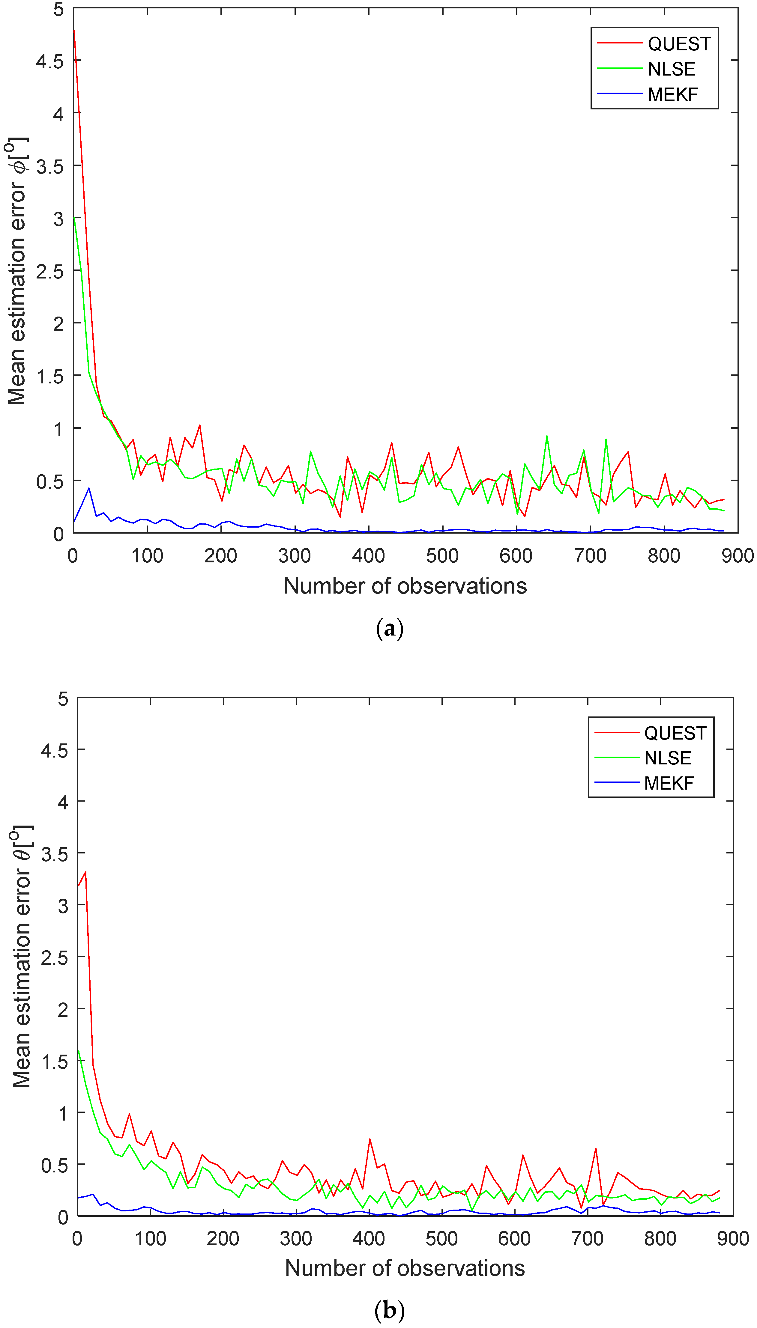
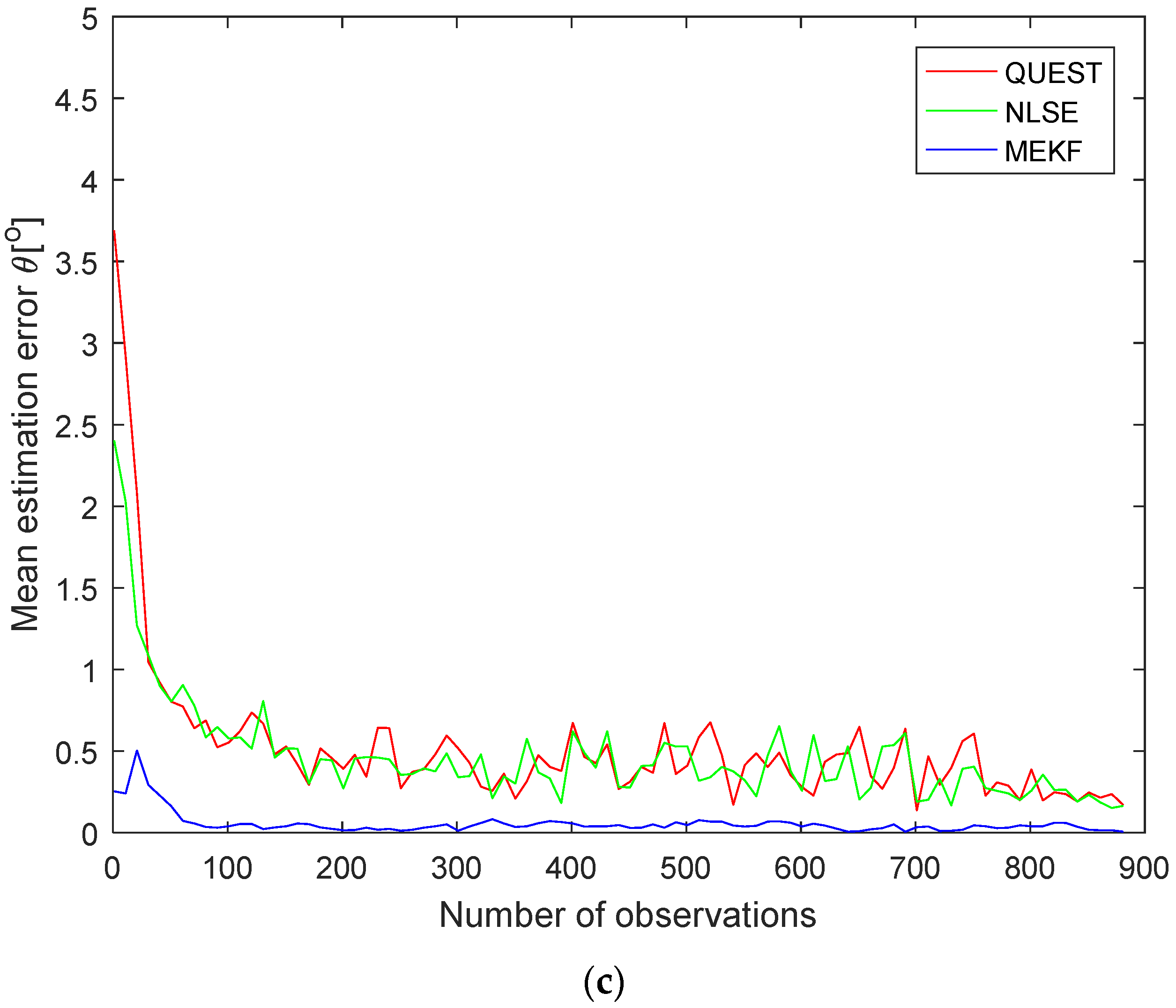
Comparing Figure 8 with Figure 9, it can be seen that the estimation error varies greatly with the number of observations. To show this fact more clearly, the mean estimation error with respect to the number of observations is illustrated in Figure 10. From these figures, we can see that the estimation error will be significantly reduced as the number of observations increases, whichever method is used. Exactly speaking, the mean estimation errors converge to about 100 observations. That is to say, along with the number of observations, the mean estimation error decreases rapidly when the number of observations is less than 100, while the improvement of the estimation accuracy becomes very limited when the number of observations is greater than 100. It also can be seen in Figure 10 that for the estimation accuracy, MEKF is the best, NLSE is the second and QUEST is the worst on the whole. The NLSE and QUEST methods will have the same accuracy when the number of observations is greater than 100.

6. Conclusions

In this contribution, the ADS-B-based satellite three-axis attitude determination was discussed. The principle of ADS-B-based attitude determination was presented first. Then, three methods were employed to solve the problem, including the deterministic method, NLSE method and MEKF method. Finally, a simulation was carried out to verify these algorithms. Based on the simulation results, it can be concluded that the ADS-B-based satellite three-axis attitude determination is available. Estimation accuracy at the degree level is possible using the NLSE method and QUEST method; they only need two ADS-B antennas. Moreover, the estimation accuracy will become higher using MEKF if a gyro is added.

Our future work will modify the MEKF method to achieve higher attitude estimation accuracy. A preliminary ideal is reformulating the observation model in MEKF and choosing the SNR measurement as the observation directly, rather than the Euler angle estimated by NLSE method. This may eliminate the error caused by the NLSE method.

References

- Ali, B.S.; Ochieng, W.Y.; Zainudin, R. An analysis and model for Automatic Dependent Surveillance Broadcast (ADS-B) continuity. GPS Solut. 2017, 21, 1841–1854. [Google Scholar] [CrossRef]
- Olive, X.; Morio, J. Trajectory clustering of air traffic flows around airports. Aerosp. Sci. Technol. 2019, 84, 776–781. [Google Scholar] [CrossRef] [Green Version]
- Leonardi, M.; Di Gregorio, L.; Di Fausto, D. Air traffic security: Aircraft classification using ADS-B message’s phase-pattern. Aerospace 2017, 4, 51. [Google Scholar] [CrossRef] [Green Version]
- Proud, S.R. Go-around detection using crowd-sourced ADS-B position data. Aerospace 2020, 7, 16. [Google Scholar] [CrossRef] [Green Version]
- Kumar, S.G.; Corrado, S.J.; Puranik, T.G.; Mavris, D.N. Classification and analysis of go-arounds in commercial aviation using ADS-B data. Aerospace 2021, 8, 291. [Google Scholar] [CrossRef]
- Hünemohr, D.; Litzba, J.; Rahimi, F. Usage Monitoring of Helicopter Gearboxes with ADS-B Flight Data. Aerospace 2022, 9, 647. [Google Scholar] [CrossRef]
- Deng, C.; Cheng, C.; Qu, T.; Li, S.; Chen, B. A Method for Managing ADS-B Data Based on a 4D Airspace-Temporal Grid (GeoSOT-AS). Aerospace 2023, 10, 217. [Google Scholar] [CrossRef]
- Roy, P.; Dawn, D. A high power fully integrated single-chip CMOS transmitter for wireless communication of unmanned aircraft system. Microw. Opt. Technol. Lett. 2017, 59, 432–439. [Google Scholar] [CrossRef]
- Zhang, J.F.; Liu, J.; Hu, R.; Zhu, H.B. Online four dimensional trajectory prediction method based on aircraft intent updating. Aerosp. Sci. Technol. 2018, 77, 774–787. [Google Scholar] [CrossRef]
- Zhang, X.; Zhang, J.J.; Wu, S.F.; Cheng, Q.; Zhu, R. Aircraft monitoring by the fusion of satellite and ground ADS-B data. Acta Astronaut. 2018, 143, 398–405. [Google Scholar] [CrossRef]
- Werner, K.; Bredemeyer, J.; Delovski, T. ADS-B over Satellite Global Air Traffic Surveillance from Space. In Proceedings of the Tyrrhenian International Workshop on Digital Communications—Enhanced Surveillance of Aircraft and Vehicles (TIWDC/ESAV), Capri, Italy, 15–16 September 2014. [Google Scholar]
- Alminde, L.K.; Kaas, K.; Bisgaard, M.; Christiansen, J.; Gerhardt, D. GOMX-1 flight experience and air traffic monitoring results. In Proceedings of the 28th Annual AIAA/USU Conference on Small Satellites, Logan, UT, USA, 2–7 August 2014. [Google Scholar]
- Gerhardt, D.; Bisgaard, M.; Alminde, L.; Walker, R.; Fernandez, M.A.; Latiri, A.; Issler, J. GOMX-3: Mission Results from the Inaugural ESA In-Orbit Demonstration CubeSat. In Proceedings of the 30th Annual AIAA/USU Conference on Small Satellites, Toulouse, France, 27–30 September 2016. [Google Scholar]
- Garcia, M.A.; Dolan, J.; Hoag, A. Aireon’s initial on-orbit performance analysis of space-based ADS-B. In Proceedings of the Integrated Communications Navigation and Surveillance Conference (ICNS), Herndon, VA, USA, 18–20 April 2017. [Google Scholar]
- Akan, D.; Rudan, I.; Ukin, S.; Bri, D. Near Real-time S-AIS: Recent Developments and Implementation Possibilities for Global Maritime Stakeholders. Sci. J. Marit. Res. 2018, 32, 211–218. [Google Scholar] [CrossRef] [Green Version]
- Zhou, K.X.; Sun, X.C.; Huang, H.; Wang, X.S.; Ren, G.W. Satellite single-axis attitude determination based on Automatic Dependent Surveillance—Broadcast signals. Acta Astronaut. 2017, 139, 130–140. [Google Scholar] [CrossRef]
- Axelrad, P.; Behre, C.P. Satellite attitude determination based on GPS signal-to-noise ratio. Proc. IEEE 1999, 87, 133–144. [Google Scholar] [CrossRef]
- Lightsey, E.G.; Madsen, J. Three-axis attitude determination using global positioning system signal strength measurements. J. Guid. Control Dyn. 2003, 26, 304–310. [Google Scholar] [CrossRef]
- Peters, D. Attitude Determination for Small Satellites Using GPS Signal-to-Noise Ratio. Master’s Thesis, University of Alaska Fairbanks, Fairbanks, AK, USA, 2014. [Google Scholar]
- Bettray, A.; Litschke, O.; Baggen, L. Multi-Beam Antenna for Space-Based ADS-B. In Proceedings of the 5th IEEE International Symposium on Phased Array Systems and Technology, Waltham, MA, USA, 15–18 October 2013. [Google Scholar]
- Yu, S.Q.; Chen, L.H.; Li, S.T.; Zhang, X. Adaptive Multi-beamforming for Space-based ADS-B. J. Navig. 2019, 72, 359–374. [Google Scholar] [CrossRef]
- Golestani, M.; Esmaeilzadeh, S.M.; Xiao, B. Fault-tolerant attitude control for flexible spacecraft subject to input and state constraint. Trans. Inst. Meas. Control. 2020, 42, 2660–2674. [Google Scholar] [CrossRef]
- Xuan-Mung, N.; Golestani, M. Energy-efficient disturbance observer-based attitude tracking control with fixed-time convergence for spacecraft. IEEE Trans. Aerosp. Electron. Syst. 2022, 1–10. [Google Scholar] [CrossRef]
- Xuan-Mung, N.; Golestani, M.; Hong, S.K. Tan-Type BLF-Based Attitude Tracking Control Design for Rigid Spacecraft with Arbitrary Disturbances. Mathematics 2022, 10, 4548. [Google Scholar] [CrossRef]
- Xuan-Mung, N.; Golestani, M.; Hong, S.K. Constrained Nonsingular Terminal Sliding Mode Attitude Control for Spacecraft: A Funnel Control Approach. Mathematics 2023, 11, 247. [Google Scholar] [CrossRef]
- Tomasi, W. Electronic Communication, 2nd ed.; Prentice Hall: Hoboken, NJ, USA, 1994; ISBN 978-013-220-062-2. [Google Scholar]
- Wahba, G. A least squares estimate of satellite attitude. SIAM Rev. 1965, 7, 409. [Google Scholar] [CrossRef]
- Shuster, M.D.; Oh, S.D. Three-axis attitude determination from vector observations. J. Guid. Control. 1981, 4, 70–77. [Google Scholar] [CrossRef]
- Chang, G.; Xu, T.; Wang, Q. Error analysis of Davenport’sq method. Automatica 2017, 75, 217–220. [Google Scholar] [CrossRef]
- Psiaki, M.L. Attitude-determination filtering via extended quaternion estimation. J. Guid. Control. Dyn. 2000, 23, 206–214. [Google Scholar] [CrossRef]
- Markley, F.L. Attitude determination using vector observations and the singular value decomposition. J. Astronaut. Sci. 1988, 36, 245–258. [Google Scholar]
- Yan, G.; Chen, R.; Weng, J. A super-fast optimal attitude matrix in attitude determination. Meas. Sci. Technol. 2021, 32, 095012. [Google Scholar]
- Lourakis, M.I. A brief description of the Levenberg-Marquardt algorithm implemented by levmar. Found. Res. Technol. 2005, 4, 1–6. [Google Scholar]
- Hartley, H.O. The modified Gauss-Newton method for the fitting of non-linear regression functions by least squares. Technometrics 1961, 3, 269–280. [Google Scholar] [CrossRef]
- Liu, B.C.; Lin, K.H. Geometric Location Techniques with SSSD in Wireless Cellular Networks: A Comparative Performance Study. In Proceedings of the VTC Spring 2008-IEEE Vehicular Technology Conference, Singapore, 11–14 May 2008; IEEE: Piscataway, NJ, USA, 2008; pp. 2720–2724. [Google Scholar]
- Shuster, M.D. The kinematic equation for the rotation vector. IEEE Trans. Aerosp. Electron. Syst. 1993, 29, 263–267. [Google Scholar] [CrossRef]
- Shieh, L.S.; Wang, H.; Yates, R.E. Discrete-continuous model conversion. Appl. Math. Model. 1980, 4, 449–455. [Google Scholar] [CrossRef]
- Zhou, K.; Huang, H.; Wang, X.; Sun, L. Magnetic attitude control for Earth-pointing satellites in the presence of gravity gradient. Aerosp. Sci. Technol. 2017, 60, 115–123. [Google Scholar] [CrossRef]
Figure 1.
Gain pattern of the double-antenna-receiving system. Only the main lobes are shown in this figure.
Figure 2.
Basic principle of ADS-B-based three-axis satellite attitude determination.
Figure 3.
Coordinate frame 3-2-1 rotation.
Figure 4.
The azimuth angle and elevation angle of the boresight vector.
Figure 5.
Helical antenna.
Figure 6.
The simulation result of the helical antenna gain pattern.
Figure 7.
The installation location and geometry configuration of two helical antennas.
Figure 8.
The number of available observations.
Figure 9.
The estimation errors of Euler angle by QUEST (a), NLSE (b) and MEKF (c) methods.
Figure 10.
Mean estimation errors of (a), (b) and (c) with respect to the number of observations.