
Effective Distance for Vortex Generators in High Subsonic Flows

Abstract
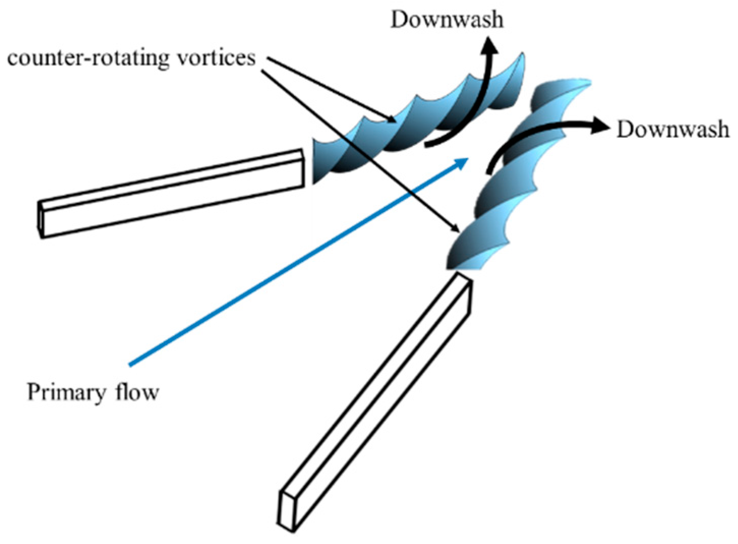
:1. Introduction
2. Experimental Setup
2.1. Transonic Wind Tunnel
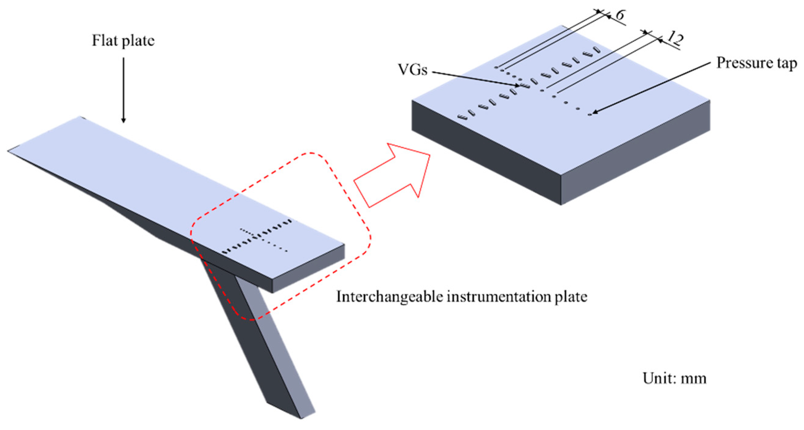
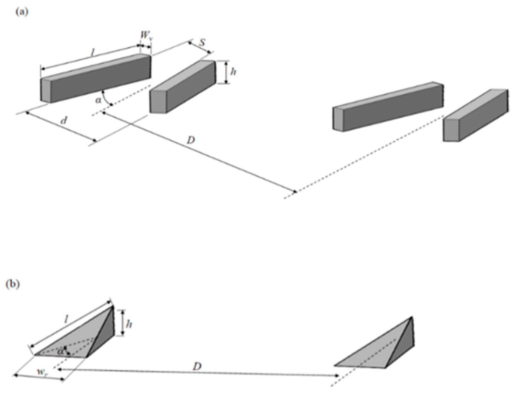
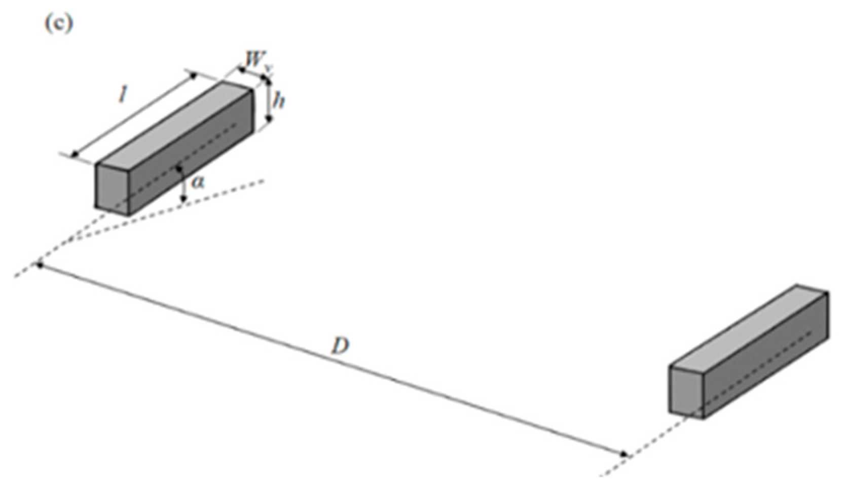
2.2. Test Model
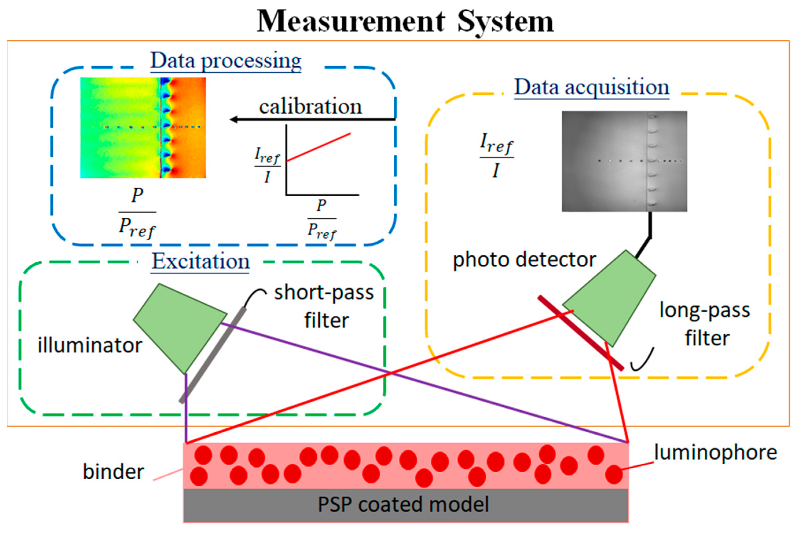
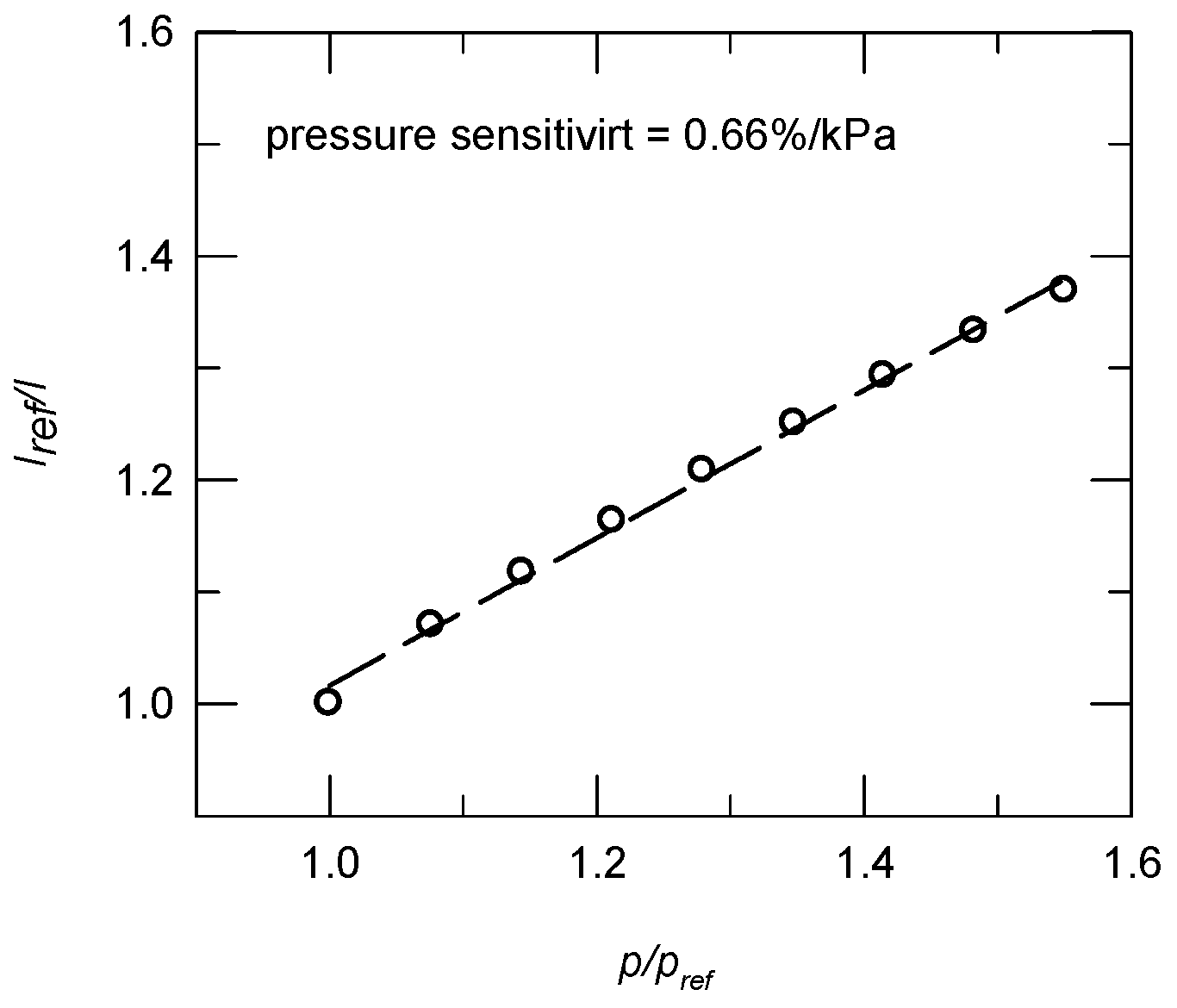
2.3. Instrumentation and Data Acquisition System
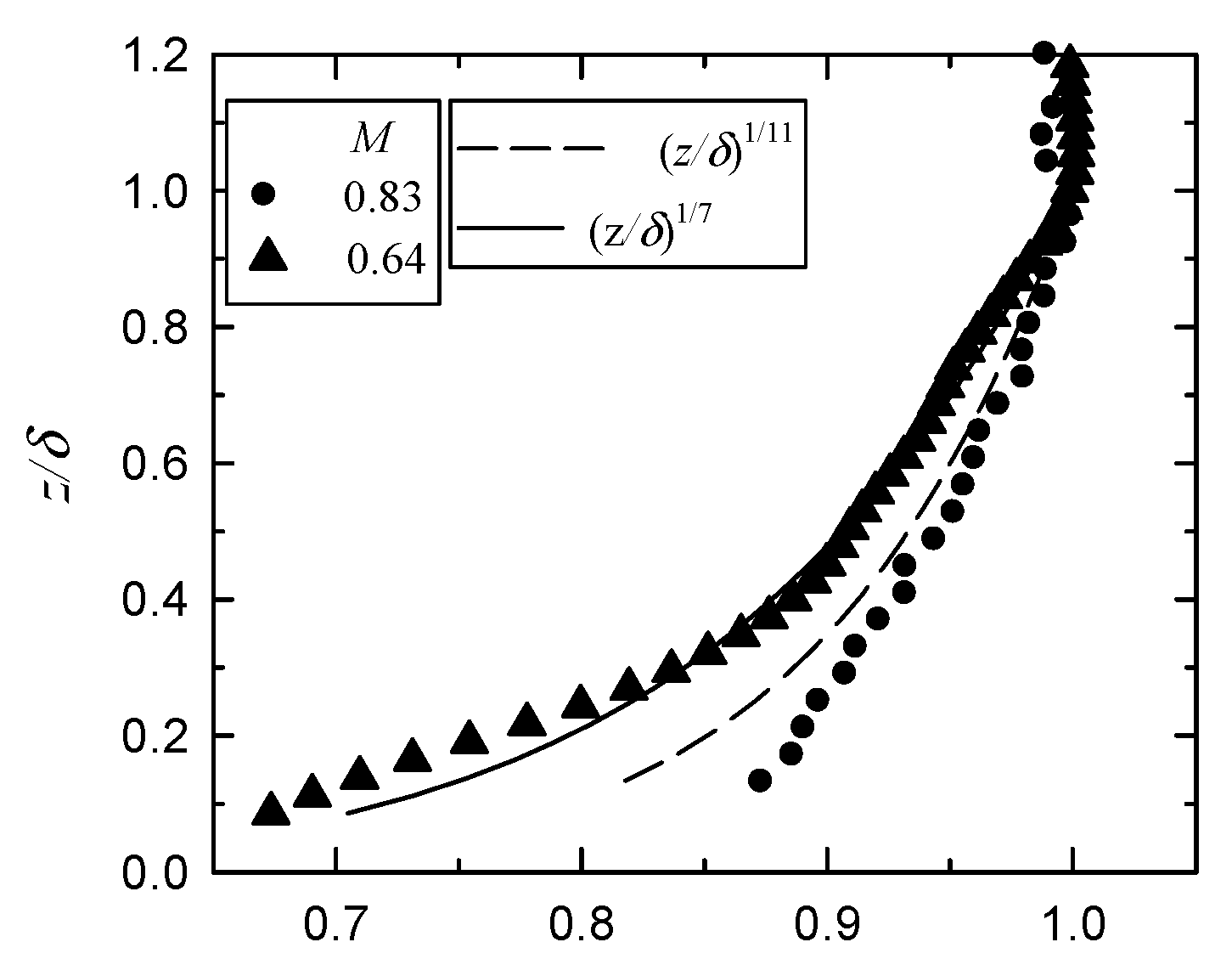
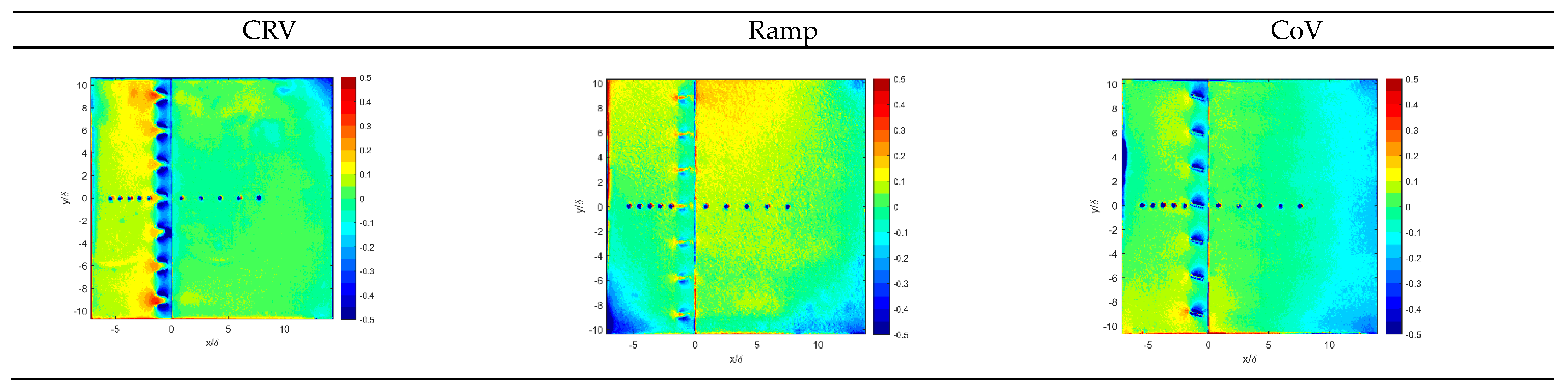
3. Results and Discussion
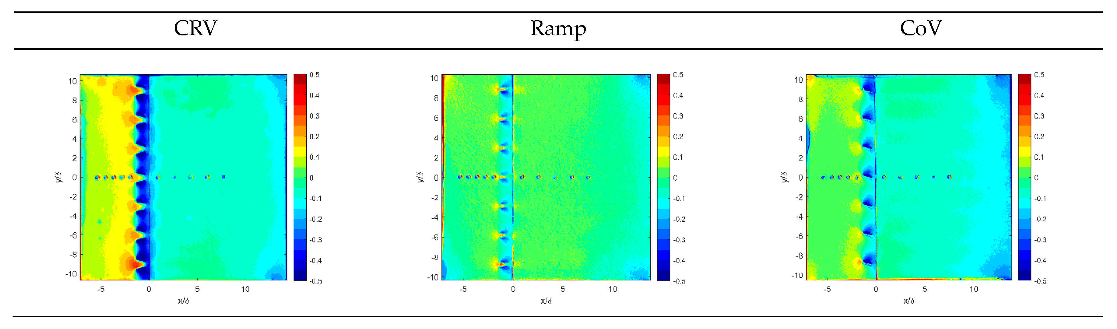
3.1. Surface Pressure Pattern
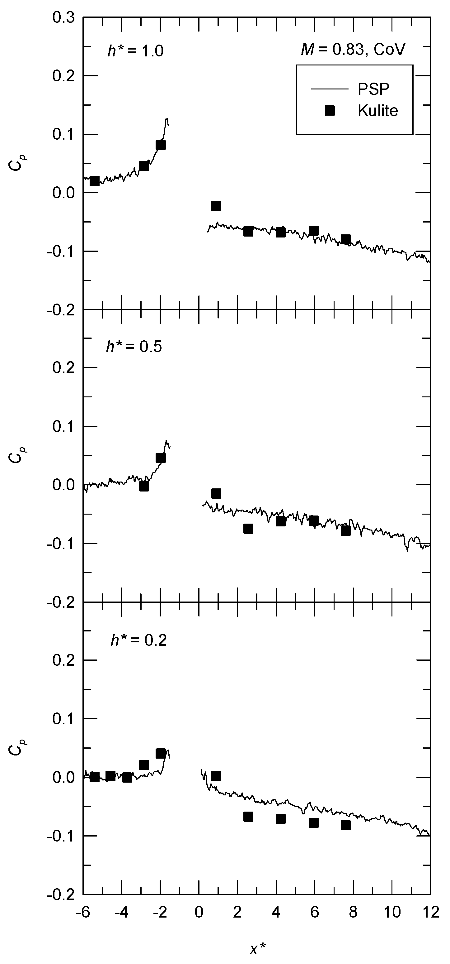
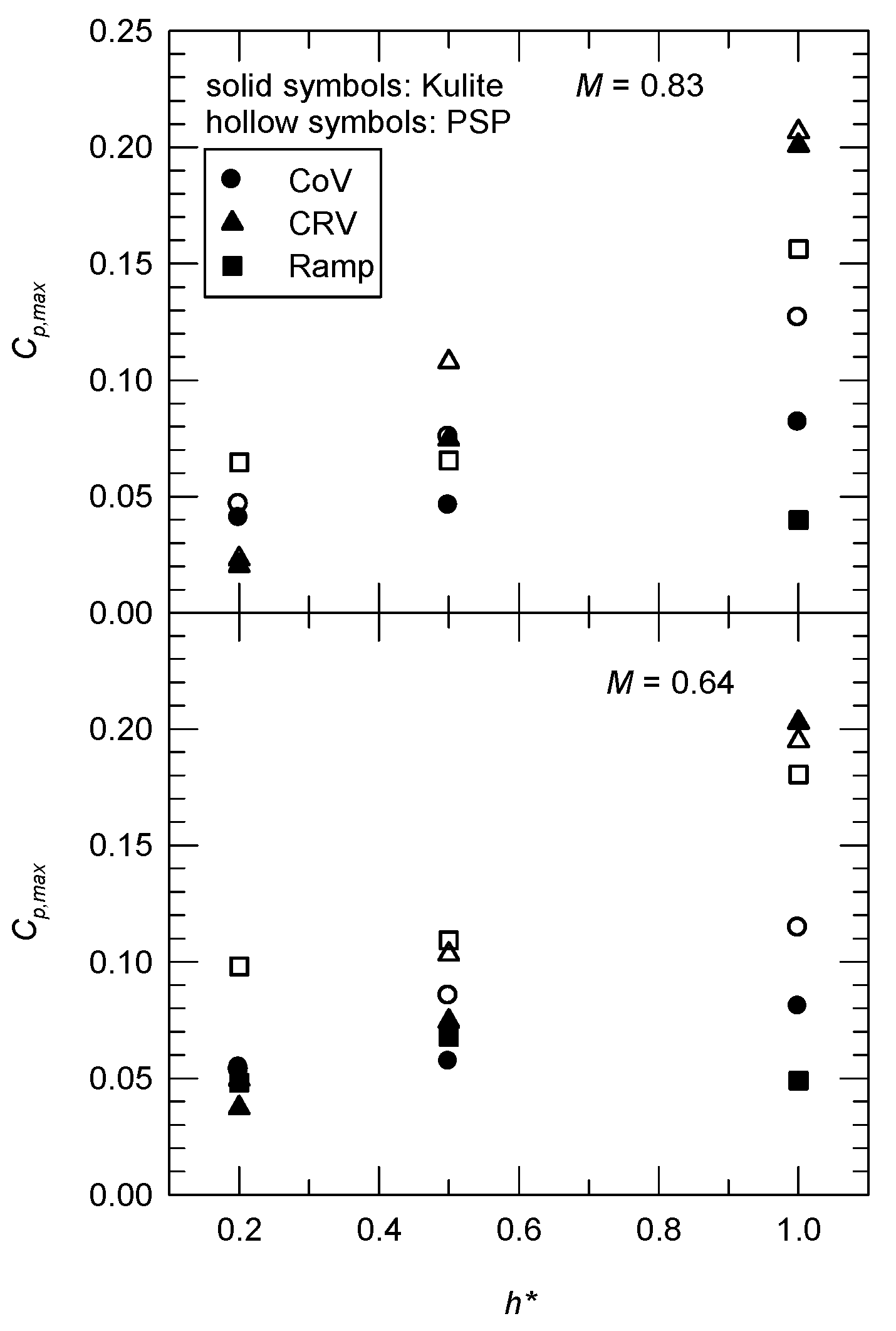
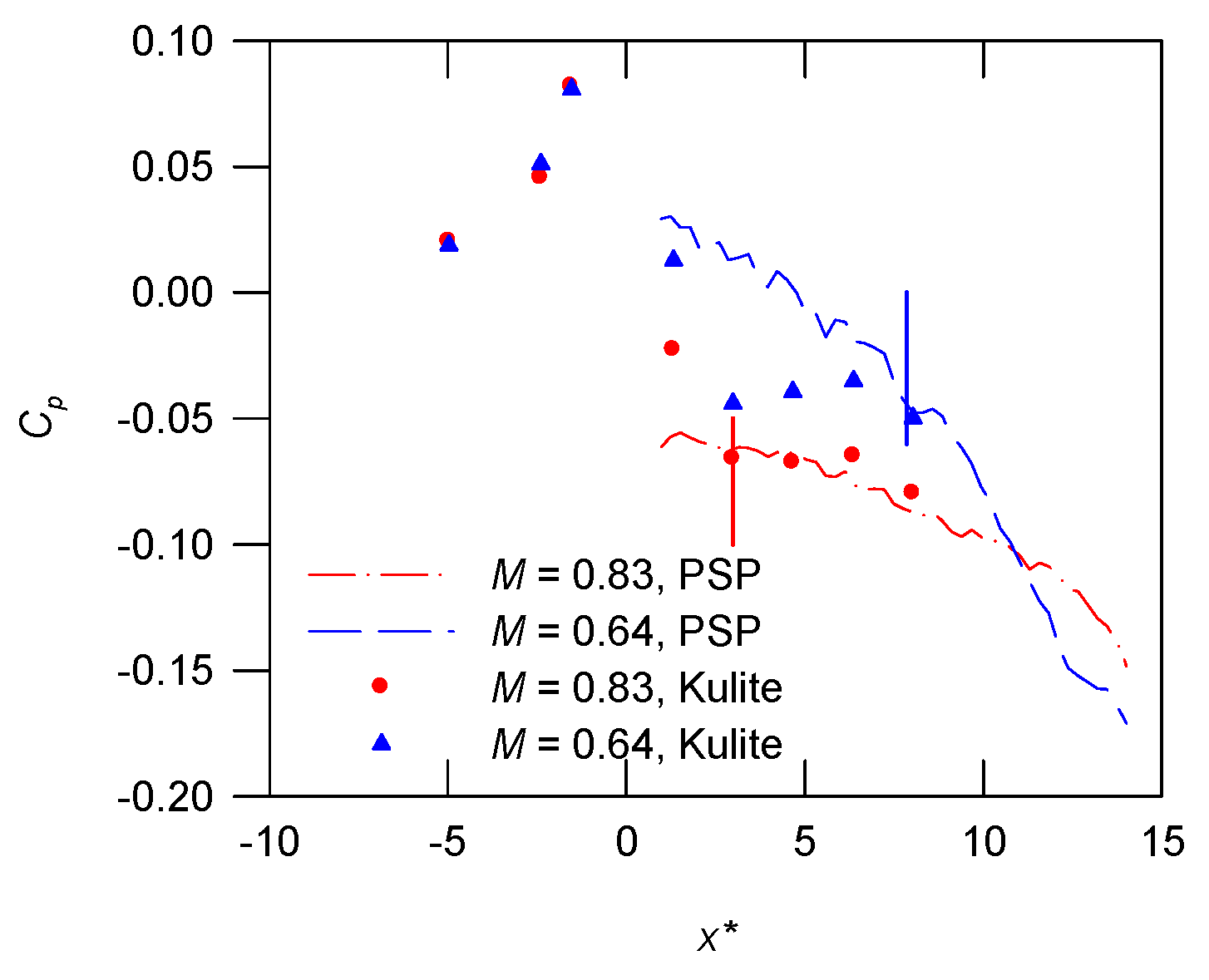
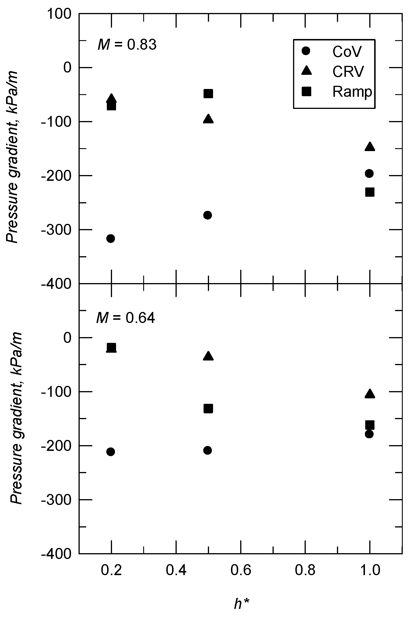
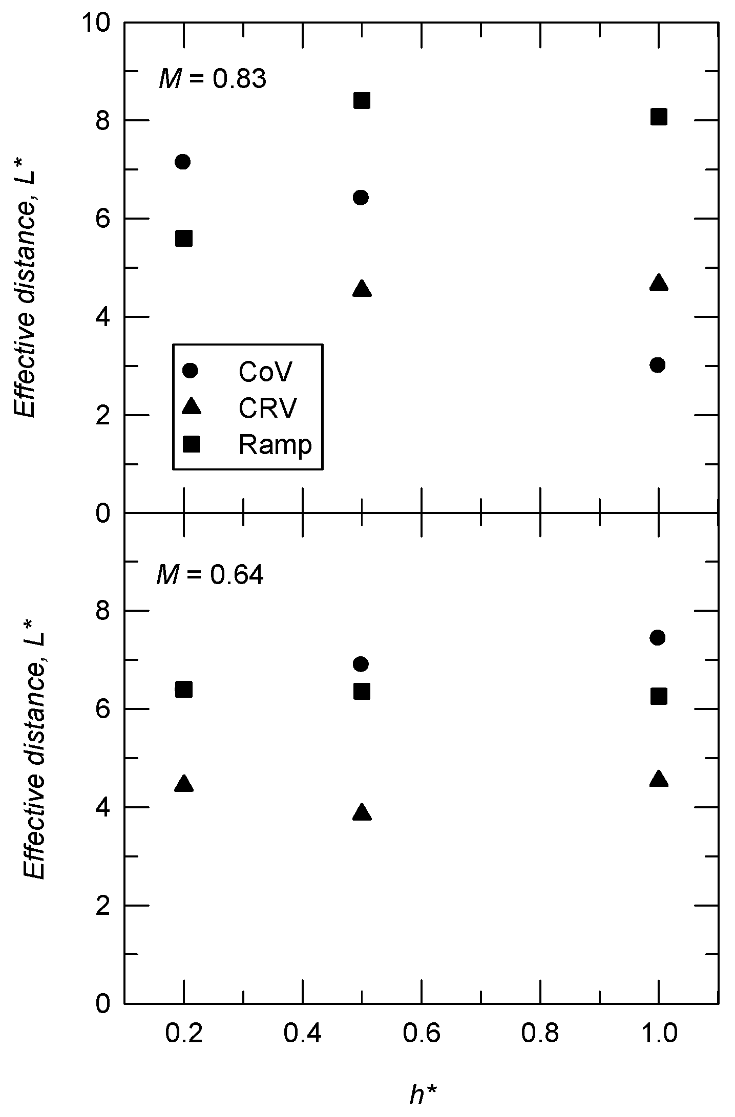
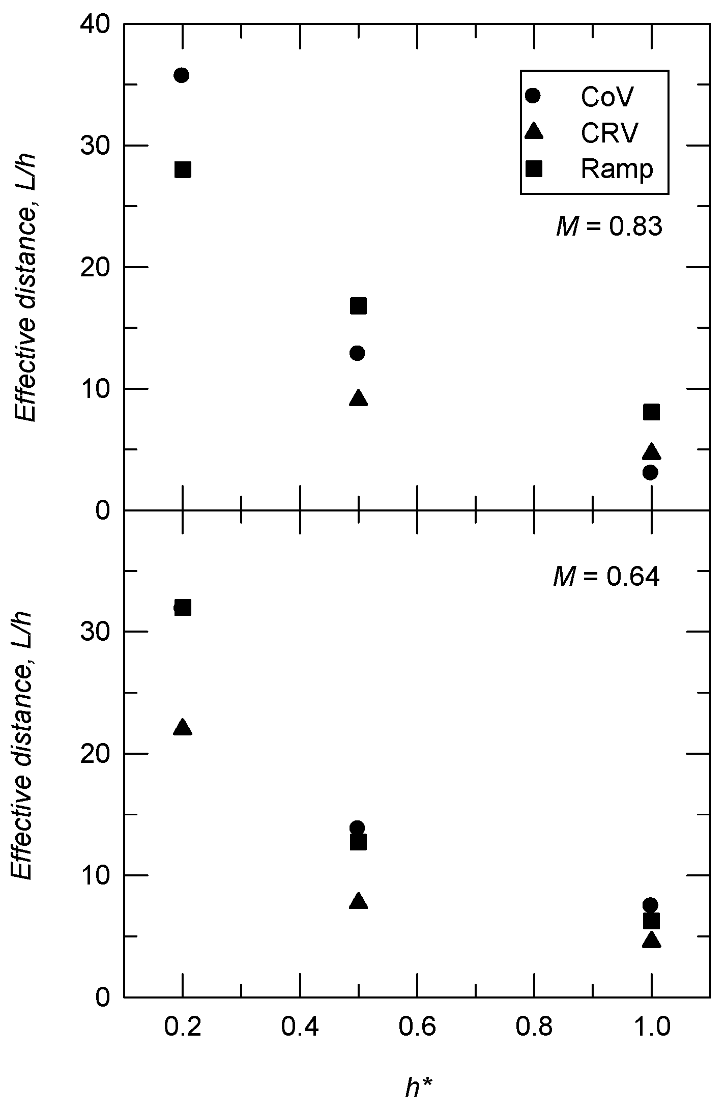
3.2. Effective Distance
4. Conclusions
Author Contributions
Funding
Data Availability Statement
Acknowledgments
Conflicts of Interest
Nomenclature
| A(T) | constant for PSP calibration curve |
| B(T) | pressure sensitivity |
| Cp | surface pressure coefficient |
| Cp,max | peak surface pressure coefficient upstream of vortex generator |
| d | front spacing of counter-rotating vortex generator |
| D | spacing between adjacent vortex generators |
| h | height of vortex generator |
| I | intensity of the emission |
| Iref | reference intensity of emission |
| h* | normalized height of vortex generator, h/δ |
| l | length of vortex generator |
| L | effective distance |
| L* | normalized effective distance, L/δ |
| M | freestream Mach number |
| po | stagnation pressure |
| pref | reference pressure (= ambient pressure) |
| q | dynamic pressure |
| s | rear spacing of counter-rotating vortex generator |
| T | temperature |
| u | velocity |
| U∞ | freestream velocity |
| w | width of vortex generator |
| x | coordinate along the centerline of model surface |
| x* | normalized streamwise distance, x/δ |
| α | angle of incidence of vortex generator |
| δ | incoming boundary-layer thickness |
| y | coordinate in spanwise direction |
| y* | normalized spanwise distance, y/δ |
| z | vertical distance from the surface |
References
- Wang, Y.; Liu, D.; Xu, X.; Li, G. Investigation of Reynolds number effects on aerodynamic characteristics of a transport aircraft. Aerospace 2021, 8, 177. [Google Scholar] [CrossRef]
- Ashill, P.R.; Fulker, J.L.; Hackett, K.C. A reviews of recent developments in flow control. Aeronaut. J. 2005, 109, 205–232. [Google Scholar] [CrossRef]
- Lin, J.C. Review of research on low-profile vortex generators to control boundary-layer separation. Prog. Aerosp. Sci. 2002, 38, 389–420. [Google Scholar] [CrossRef]
- Lin, J.C.; Robinson, S.K.; Mcghee, R.J.; Valarezo, W.O. Separation control on high-lift airfoils via micro-vortex generators. J. Aircr. 1994, 31, 1317–1323. [Google Scholar] [CrossRef]
- Lee, S.; Loth, E. Effect of Mach number on flow past microramps. AIAA J. 2011, 49, 97–110. [Google Scholar] [CrossRef]
- Gaqeik, M.; Nies, J.; Klioutchnikov, I.; Oliver, H. Pressure wave damping in transonic airfoil flow by means of micro vortex generators. Aerosp. Sci. Technol. 2018, 81, 65–77. [Google Scholar] [CrossRef]
- Titchener, N.; Babinsky, H. A review of the use of vortex generators for mitigating shock-induced separation. Shock Waves 2015, 25, 473–494. [Google Scholar] [CrossRef] [Green Version]
- Bur, R.; Coponet, D.; Carpels, Y. Separation control by vortex generator devices in a transonic channel flow. Shock Waves 2009, 19, 521–530. [Google Scholar] [CrossRef]
- Panaras, A.G.; Lu, F.K. Micro-vortex generators for shock wave/boundary layer interactions. Prog. Aerosp. Sci. 2015, 74, 16–47. [Google Scholar] [CrossRef]
- Lee, S.; Loth, E. Impact of ramped vanes on normal shock boundary-layer interaction. AIAA J. 2012, 50, 2069–2079. [Google Scholar] [CrossRef]
- Su, K.C.; Chung, K.M.; Isaev, S. Separation control for a transonic convex-corner flow using ramp-type vortex generators. Int. J. Aerosp. Eng. 2022, 2022, 4048490. [Google Scholar] [CrossRef]
- Singh, N.K. Numerical simulation of flow behind vortex generators. J. Appl. Fluid Mech. 2019, 12, 1047–1061. [Google Scholar] [CrossRef]
- Lu, F.K.; Li, Q.; Liu, C. Microvortex generators in high-speed flow. Prog. Aerosp. Sci. 2012, 53, 30–45. [Google Scholar] [CrossRef]
- Baydar, E.; Lu, F.K.; Slater, J.W. Vortex generators in a two-dimensional external-compression supersonic inlet. J. Prop. Power 2018, 34, 521–538. [Google Scholar] [CrossRef] [Green Version]
- Pearcey, H.H. Shock-induced separation and its prevention by design and boundary layer control. In Boundary Layer and Flow Control: Its Principles and Application; Pergamon Press: Oxford, UK, 1961; Volume 2, pp. 1166–1344. [Google Scholar]
- Chung, K.C.; Su, K.C.; Chang, K.C. The effect of vortex generators on shock-induced boundary layer separation in a transonic convex-corner flow. Aerospace 2021, 8, 157. [Google Scholar] [CrossRef]
- Chung, K.M. Unsteadiness of transonic convex-corner flows. Exp. Fluids 2004, 37, 917–922. [Google Scholar] [CrossRef]
- Chung, K.M.; Huang, Y.X.; Lin, C.Y.; Wu, Y.T. Surface pressure measurements on a forebody using pressure-sensitive paint. J. Aeronaut. Astronaut. Aviat. 2021, 53, 369–374. [Google Scholar]
- Chung, K.M.; Huang, Y.X. Global visualization of compressible swept convex-corner flow using pressure-sensitive paint. Aerospace 2021, 8, 106. [Google Scholar] [CrossRef]
- Running, C.L.; Juliano, T.J. Global measurements of hypersonic shock-wave/boundary-layer interactions with pressure-sensitive paint. Exp. Fluids 2021, 62, 91. [Google Scholar] [CrossRef]
- Wei, C.; Zuo, C.; Liao, X.; Li, G.; Jiao, L.; Peng, D.; Liang, L. Simultaneous pressure and displacement measurement on helicopter rotor blades using a binocular stereophotogrammetry PSP system. Aerospace 2022, 9, 292. [Google Scholar] [CrossRef]
- Bell, J.H.; Schairer, E.T.; Hand, L.A.; Mehta, R.D. Surface pressure measurements using luminescent coatings. Annu. Rev. Fluid Mech. 2001, 33, 155–206. [Google Scholar] [CrossRef]
- Huang, C.Y.; Lin, Y.F.; Huang, Y.X.; Chung, K.M. Pressure-sensitive paint measurements with temperature correction on the wing of AGARD-B under transonic flow conditions. Meas. Sci. Technol. 2021, 32, 094001. [Google Scholar] [CrossRef]


| Parameters | Value |
|---|---|
| h/δ | 0.2, 0.5, 1.0 |
| l/δ | 1.0 |
| D/δ | 3.0 |
| wv/δ | 0.2 |
| wr/δ | 0.5 |
| s/δ | 0.5 |
| d/δ | 1.0 |
| α | 15° |
Disclaimer/Publisher’s Note: The statements, opinions and data contained in all publications are solely those of the individual author(s) and contributor(s) and not of MDPI and/or the editor(s). MDPI and/or the editor(s) disclaim responsibility for any injury to people or property resulting from any ideas, methods, instructions or products referred to in the content. |
© 2023 by the authors. Licensee MDPI, Basel, Switzerland. This article is an open access article distributed under the terms and conditions of the Creative Commons Attribution (CC BY) license (https://creativecommons.org/licenses/by/4.0/).
Share and Cite
Chung, P.-H.; Huang, Y.-X.; Chung, K.-M.; Huang, C.-Y.; Isaev, S. Effective Distance for Vortex Generators in High Subsonic Flows. Aerospace 2023, 10, 369. https://doi.org/10.3390/aerospace10040369
Chung P-H, Huang Y-X, Chung K-M, Huang C-Y, Isaev S. Effective Distance for Vortex Generators in High Subsonic Flows. Aerospace. 2023; 10(4):369. https://doi.org/10.3390/aerospace10040369
Chicago/Turabian StyleChung, Ping-Han, Yi-Xuan Huang, Kung-Ming Chung, Chih-Yung Huang, and Sergey Isaev. 2023. "Effective Distance for Vortex Generators in High Subsonic Flows" Aerospace 10, no. 4: 369. https://doi.org/10.3390/aerospace10040369