A Method for Satellite Component Health Assessment Based on Multiparametric Data Distribution Characteristics

Abstract

This research presents a novel data-based multi-parameter health assessment method to meet the growing need for the in-orbit health assessment of satellite components. This method analyzed changes in component health status by calculating distribution deviations and variation similarities in real-time operational data. Firstly, a single-parameter health state description method based on data distribution characteristics was presented. Secondly, the main health characteristic parameters were selected by mechanistic analysis and expert experience. The CRITIC method and the entropy weighting method were fused to assign reasonable weights and establish a multi-parameter component health assessment model. Then, the feasibility of a component health assessment algorithm based on data distribution characteristics was verified using real telemetry data from satellites. Finally, to verify the rationality of the presented health assessment algorithm, the results were compared with the pre-processed original data using empirical mode decomposition. The experimental results show that the method can accurately describe the change trend of the health status of the components. It proves that the method can be effectively used for the real-time health condition assessment and monitoring of satellite components.

1. Introduction

Satellites have the important task of promoting national economy, national defense security, and scientific research development. The in-orbit health assessment of satellite components can make use of limited computing resources for real-time information processing, improving the level of self-management of satellites in orbit. Concurrently, it furnishes a foundation for decision-making regarding in-orbit maintenance, system-level and full-satellite health assessment, and telemetry transmission optimization [1]. The delicate structure of spacecraft components [2,3] and the complex orbital environment all pose significant challenges for satellite components to undergo in-orbit health assessment research [4,5].

With the rapid development of the aerospace industry and the increase in data from long-term satellite operations in orbit, data-based health assessment research has become a hot topic. Researchers have gradually applied intelligent algorithms such as feature extraction, data fusion, and transfer learning to the research of health assessment of satellite components. The research directions can be divided into three main categories: remaining life, probability of fault, and degree of condition deviation. Of these three directions, assessing components by predicting their remaining life [6,7,8,9,10,11] and their probability of fault [12,13,14,15,16] is currently the dominant health assessment perspective [17]. Islam et al. [18] utilized the LSTM prediction method to predict the remaining service life of satellite reaction wheels. By utilizing a large amount of satellite data, Huang et al. [19] established a degradation model to predict the remaining lifetime of in-orbit satellites. Song et al. [20] proposed a hybrid method combining an IDN-AR model and PF algorithm to improve the accuracy of predicting the remaining life of lithium-ion batteries in satellites. Islam et al. [21] used time-series forecasting methods to predict the faults of satellite reaction wheels. Suo et al. [22] proposed a data-driven fault diagnosis strategy combining the fast iterative method and support vector machine, and verified its effectiveness using satellite power system data. Varvani Farahani et al. [23] proposed an enhanced data-driven fault diagnosis method based on the support vector machine approach, which can achieve high-precision detection of the faults in satellite gyros. Chen et al. [24] considered the performance degradation of actuators and used the transfer learning method for the fault detection of complex systems.

However, component lifetime is heavily influenced by random environments and is difficult to verify. The analysis of component fault probability requires a large sample of faults, which is often difficult to obtain [25]. The health assessment of components through the degree of state deviation is a novel research perspective proposed in recent years. It does not rely on a priori knowledge, has low sample requirements, and is easy to validate. However, the study of in-orbit real-time health assessment for satellite components with complex periodic changes, precise structure, and challenging mechanism modeling is still in its early stages [26].

In terms of the selection of characteristic parameters for health assessment research, most of the current research uses a single parameter for analysis. Although a single key characteristic parameter reflecting performance degradation selected through expert experience can show the trend of the component’s health status, it is difficult to fully describe the working characteristics of the component with a single parameter. A reasonable weighting must be assigned when considering multiple parameters. There are two main types of methods for assigning weights: subjective weighting methods [27,28] and objective weighting methods [29,30,31]. Different weighting methods have their own advantages and disadvantages. The results of weight assignment directly affect the final results of the health assessment. Therefore, appropriate methods must be adopted for the weighting of multiple parameters. The Criteria Importance through Intercriteria Correlation (CRITIC) method determines weights based on the strength of comparison between different parametric data and the correlation between parameters, but does not reflect the degree of dispersion of the individual parametric data themselves [32,33]. The entropy weighting method is a multicriteria decision analysis method mainly used for determining the weights of parameters. Its basic idea is to determine the weights of each parameter in the parameter set by calculating the information entropy value of each parameter. However, it does not take into account the relationships between different parameters [34]. Combining the CRITIC method with the entropy weight method can make the weight assignment results more objective, reasonable, and reliable.

This study focused on the in-orbit health assessment of key satellite components. It presented a new universal health assessment method based on the multiparametric data distribution characteristics from the perspective of describing the deviation of component health status. The main innovations are as follows: (1) rearranging the operational data, and then characterizing the operational data from the perspective of data distribution deviations (DDD) and similarity of operational data changes (SOC). This addresses the difficulty of analyzing trends in state change with short-term data; (2) fusing the CRITIC weighting method and the entropy weighting method to assign weights to the health characteristic parameters selected using expert experience and mechanism analysis. This approach addresses the difficulty of fully describing the operating characteristics of a component with a single parameter and avoids excessive subjective influences. This leads to a component health assessment model; and (3) the empirical mode decomposition algorithm, which is used to extract the trends of DDD, differences in the similarity of operational data changes (DSOC), and original data after preprocessing. The validity and reliability of the method was verified by comparison and analysis.

2. Problem Formulation and Overall Approach

2.1. Problem Formulation

Firstly, to calculate the degree of deviation from the component condition, the main health characteristic parameters ${\mathsf{\xi }}_{\mathrm{i}}$ need to be determined. It is also necessary to determine the ideal health state benchmark for each parameter through reasonable indicators. At this moment, it is a challenge to describe the variation in covariate data accurately, reasonably, and completely. The algorithms for measuring the differences in data distribution only compare at the numerical level. They ignore the case where the data are essentially the same and the differences in data variation are significant. Therefore, the degree of deviation from the parametric state needs to be described in combination with DDD ${\mathrm{f}}_1\left(\mathsf{\xi }\right)$ and SOC ${\mathrm{f}}_2\left(\mathsf{\xi }\right)$.

Secondly, it is essential to carry out a multiparametric health assessment with a reasonable weighting. The selection of feature parameters ${\mathsf{\xi }}_{\mathrm{i}}$ often relies on expert experience and is not immune to the influence of subjectivity. The use of subjective weight allocation methods such as traditional hierarchical analysis can lead to excessive subjectivity and unreliable results. Thus, a reasonable approach is needed to determine the weight ${\mathrm{w}}_{\mathrm{i}}$ of the parameter ${\mathsf{\xi }}_{\mathrm{i}}$. This leads to a model ${\mathrm{f}}_1\left(\mathsf{\xi }\right)$ for the calculation of multiparametric DDD and a model ${\mathrm{f}}_2\left(\mathsf{\xi }\right)$ for multiparametric SOC.

$${\mathrm{f}}_1{\left(\mathsf{\xi }\right)=\mathrm{w}}_1{\mathrm{f}}_1{(\mathsf{\xi }}_1{) + \mathrm{w}}_2{\mathrm{f}}_1{(\mathsf{\xi }}_2) + \cdots { + \mathrm{w}}_{\mathrm{n}}{\mathrm{f}}_1{(\mathsf{\xi }}_{\mathrm{n}})$$

(1)

$${\mathrm{f}}_2{\left(\mathsf{\xi }\right)=\mathrm{w}}_1{\mathrm{f}}_2{(\mathsf{\xi }}_1{) + \mathrm{w}}_2{\mathrm{f}}_2{(\mathsf{\xi }}_2) + \cdots { + \mathrm{w}}_{\mathrm{n}}{\mathrm{f}}_2{(\mathsf{\xi }}_{\mathrm{n}})$$

(2)

Finally, the variation in component health status levels relies on the determination of thresholds. The historical data test is used to classify DDD into thresholds ${\mathrm{H}}_{1\mathrm{i}}$ and ${\mathrm{H}}_{2\mathrm{i}}$ corresponding to SOC. Then, the health status levels ${\mathrm{L}}_1$ and ${\mathrm{L}}_2$ are determined according to the calculation results of ${\mathrm{f}}_1\left(\mathsf{\xi }\right)$ and ${\mathrm{f}}_2\left(\mathsf{\xi }\right)$ based on ${\mathrm{H}}_{1\mathrm{i}}$ and ${\mathrm{H}}_{2\mathrm{i}}$, respectively. Combining the two results determines the final health status class of the component, we obtain the following:

$${\mathrm{L}=\min (\mathrm{L}}_1{,\mathrm{L}}_2)$$

(3)

Based on the abovementioned issues and analysis, a combination of DDD and SOC can be considered. A multiparameter component health condition assessment model was established by determining the weight of the main health characteristic parameters in a suitable weighting method. Finally, historical data testing was used to determine the level thresholds, allowing for the real-time in-orbit health assessment of key satellite components.

2.2. Overall Approach

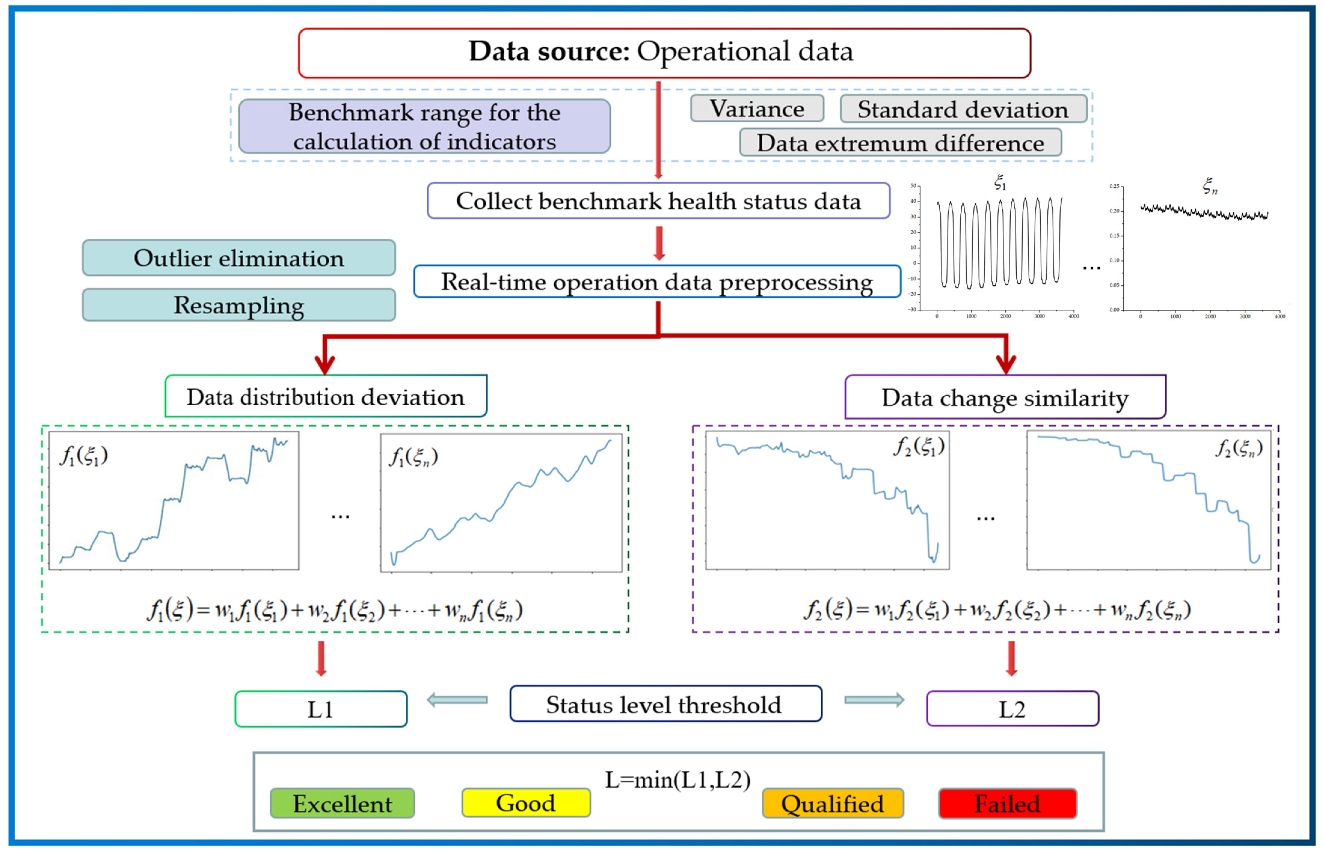
The component health assessment method presented in this paper can be divided into two main parts: offline training and online assessment. In the offline training phase, historical telemetry data of components with a full life cycle were used for testing, benchmarking, and weighting after preprocessing. Data preprocessing includes outlier elimination, resampling, and data completion [35]. Then, a large number of component history data were used to determine the appropriate thresholds for DDD and SOC at different health status levels. The parameter weights and level thresholds were saved for online assessment. The online assessment stage started with the collection of health benchmark data. Afterwards, the multiparameter-integrated DDD and SOC were calculated separately from the real-time operational data. The corresponding health status levels for each of the two were determined on the basis of thresholds. The final health status of the component was then determined according to the “short board theory”. Of the two, the online assessment process is shown in Figure 1.

3. A Single-Parameter Health Assessment Method Based on Data Distribution Characteristics

3.1. Selection and Benchmarking of Component Health Characteristic Parameters

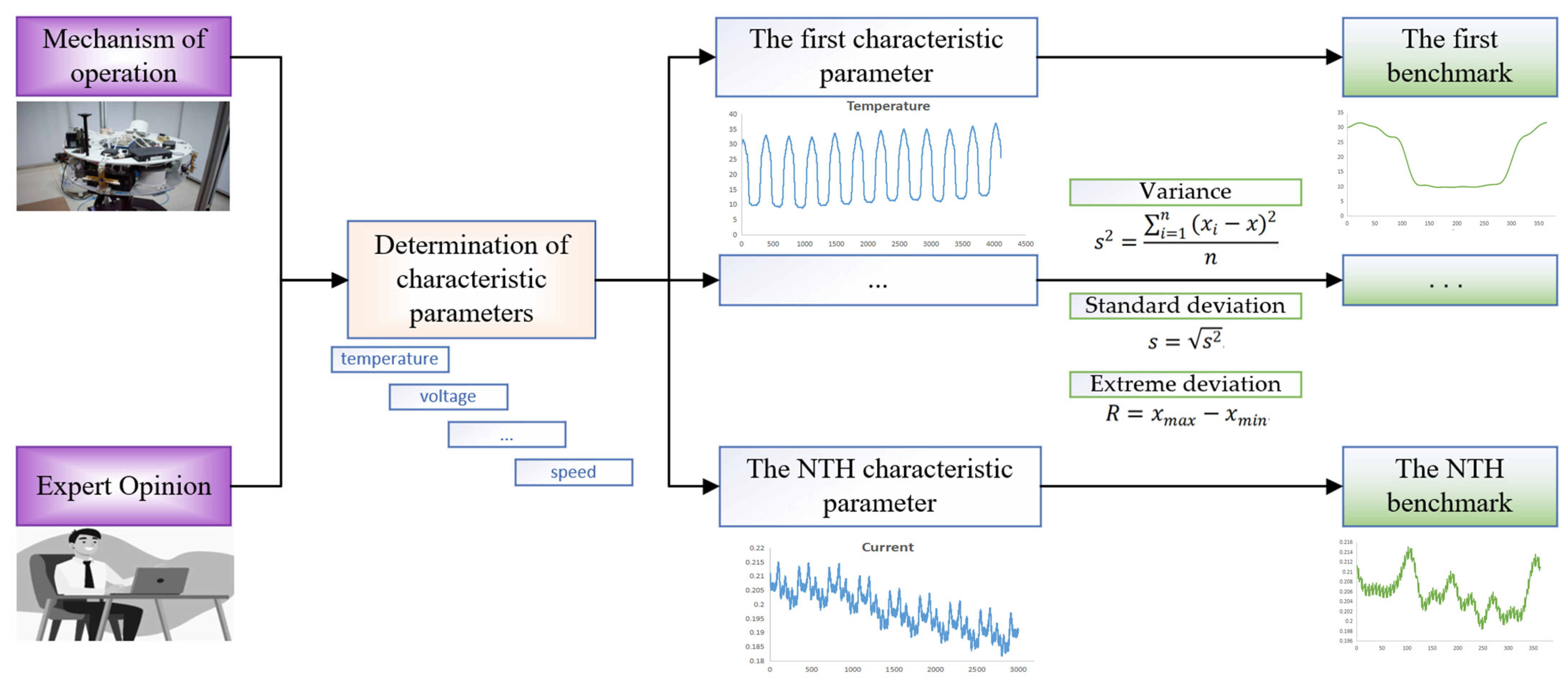
To carry out a component health assessment study, it is necessary to first select the main health characteristic parameters that reflect changes in the health status of the component. The selection of health state characteristic parameters is based on two main considerations: (1) the analysis of the working mechanism: by analyzing the working mechanism of the component, the main health characteristic parameters that reflect the changes in the health status are selected. (2) Referring to expert experience: experts in the field have studied the target component for a long time and are familiar with the parameters that characterize the health status of the component. Therefore, reference to expert opinion can considerably improve the validity and relevance of the parameters selected for assessment.

Describing the degree of deviation of a parameter must determine the health state benchmark for each parameter, which is a difficult task. Historical data from similar satellites can be analyzed to determine the benchmark range, which facilitates the subsequent real-time in-orbit health assessments of the satellites. For data where satellite components exhibit complex cyclical changes, no performance degradation or fault in the initial state of smooth operation of the component, the first full cycle or the first few full cycles can be selected as the health status benchmark. First, the first few cycles are preprocessed with outlier elimination, resampling, and data completion. Then, the variance, standard deviation, and extreme deviation of the operational data are used to quantify the most stable period of the component’s operation as a benchmark.

The aforementioned method is illustrated in Figure 2.

From the abovementioned analysis, the first prerequisite for the application of this method is clear: health benchmark data need to be collected in advance and no health assessment is carried out at this stage. Any abnormalities in the operational data of the component in the first cycle are considered as initial configuration problems or initial faults of the component. Long-term health status monitoring and assessment are not carried out.

3.2. Single Parametric Deviation Calculation Based on Data Distribution

This study presented a method for describing the health status of parametric data based on the combination of DDD and SOC. The maximum mean discrepancy (MMD) algorithm was used to calculate the distribution discrepancy between real-time operational data and benchmark data. The Pearson correlation coefficient was used to calculate the similarity of change between operational data and benchmark data after rearrangement.

MMD enables the accurate calculation of the variation in data distribution deviation. However, there are two drawbacks: (1) its inability to measure the difference between same-value data changes, and (2) its insensitivity to local data changes. The Pearson correlation coefficient has interpretability, robustness, and a hypothesis-testing process. Meanwhile, the range of its results allows it to compare the correlation of different datasets without being affected by the size of the dataset. The advantages of the Pearson correlation coefficient calculations are as follows: (1) the accurate measurement of data-change similarity, and (2) sensitivity to local data changes and the ability to capture initial anomalous data in a timely manner. However, factors that do not affect change similarity, such as amplitude, cannot be measured. The two approaches measure the variation of component data from different perspectives. The combination of DDD and SOC provides an accurate, complete, and reasonable description of the variation of data distribution.

3.2.1. Data Distribution Deviations

The maximum mean discrepancy (MMD) is an algorithm that has been widely used in migration learning in recent years. It can characterize data distributions: the maximum of the difference between the expectations of two distributions is mapped by an arbitrary function $\mathrm{f}$ in a well-defined function F [36,37,38]. It is primarily used to measure the distance between the distributions of two different, but related, random variables. The MMD measures distance by calculating arbitrary order moments for two variables. If the results are the same, the distribution is consistent, and the distance is 0. If they are different, the distance is measured by the maximum difference.

The basic definition formula is as follows:

$$\mathrm{MMD}[\mathrm{F}, \mathrm{p}, \mathrm{q}]=\begin{array}{c}\sup \\ \mathrm{f}\in \mathrm{F}\end{array}({\mathrm{E}}_{\mathrm{p}}\mathrm{f}\left(\mathrm{x}\right))-{ \mathrm{E}}_{\mathrm{q}}\mathrm{f}(\mathrm{y}))$$

(4)

The meaning of this equation is to find a mapping function that maps a variable to a higher dimensional space. The difference between the expectations of the two random variables of the distribution after mapping is called Mean Discrepancy. Then, the upper bound of this Mean Discrepancy is determined, the maximum value of which is the MMD.

The key to MMD is to find a suitable φ(x) as a mapping function, but the target mapping function varies with the task and is difficult to pick or define. Therefore, the kernel trick is used and the key to the kernel trick is to find the inner product of two vectors without explicitly representing the mapping function [39]. The MMD is squared, simplified to obtain the inner product, and expressed as a kernel function. After a derivative calculation, the MMD algorithm can be reduced to matrix form, as follows [40,41]:

MMD = tr (KL)

(5)

$$\mathrm{K}=\left[\begin{array}{cc}{\mathrm{K}}_{\mathrm{s},\mathrm{s}}& {\mathrm{K}}_{\mathrm{s},\mathrm{t}}\\ {\mathrm{K}}_{\mathrm{t},\mathrm{s}}& {\mathrm{K}}_{\mathrm{t},\mathrm{t}}\end{array}\right]$$

(6)

$${\mathrm{L}}_{\mathrm{ij}}=\{\begin{array}{cc}\frac{1}{{\mathrm{n}}^2}& {\mathrm{x}}_{\mathrm{i}}{,\mathrm{x}}_{\mathrm{j}}\in {\mathrm{X}}_{\mathrm{s}}\\ \frac{1}{{\mathrm{m}}^2}& {\mathrm{x}}_{\mathrm{i}}{,\mathrm{x}}_{\mathrm{j}}\in {\mathrm{X}}_{\mathrm{t}}\\ -\frac{1}{\mathrm{mn}}& \mathrm{otherwise}\end{array}$$

(7)

In Equation (6), the matrix K represents the kernel matrix computed by the Gaussian kernel function. In Equation (7), n represents the number of samples in the source domain, while m represents the number of samples in the target domain.

For the results of the MMD calculation, the health degree of the data distribution deviations (HDDD) can be defined as Equation (8):

$$\mathrm{HDDD}=\frac{2}{{1 + \mathrm{e}}^{\mathrm{DDD}}}=\frac{2}{{1 + \mathrm{e}}^{\mathrm{MMD}}}$$

(8)

3.2.2. Similarity of Operational Data Changes

Calculating data similarity is generally considered in terms of operational data variation. The difference in sample change is described by calculating the Pearson correlation coefficient. The Pearson correlation coefficient between two variables is defined as the quotient of the covariance and standard deviation between the two variables [42,43]:

$${\mathsf{\rho }}_{\mathrm{X},\mathrm{Y}}=\frac{\mathrm{cov}(\mathrm{X},\mathrm{Y})}{{\mathsf{\sigma }}_{\mathrm{X}}{\mathsf{\sigma }}_{\mathrm{Y}}}=\frac{\mathrm{E}\left[\right(\mathrm{X}-{\mathsf{\mu }}_{\mathrm{X}}\left)\right(\mathrm{Y}-{\mathsf{\mu }}_{\mathrm{Y}}\left)\right]}{{\mathsf{\sigma }}_{\mathrm{X}}{\mathsf{\sigma }}_{\mathrm{Y}}}$$

(9)

In Equation (9), the numerator is the covariance of two variables. Covariance is the degree to which two variables vary together when they are randomly changing. The denominator in the equation is the product of the standard deviations of each variable. Standard deviation is used to measure the variability of a variable, which is the square root of the average of the squared deviations of each data point from the mean.

For Pearson calculations, the difference between the real-time operational data changes and the benchmark data changes of a component can be defined as Equation (10):

$$\mathrm{DSOC}=1-\mathrm{SOC}=1-{\mathsf{\rho }}_{\mathrm{X},\mathrm{Y}}$$

(10)

It should be noted that if the data changes are negatively correlated, that is, SOC < 0, it indicates a fault or anomaly. Therefore, when the DSOC result is greater than 1, it also indicates that the component’s health status is very poor.

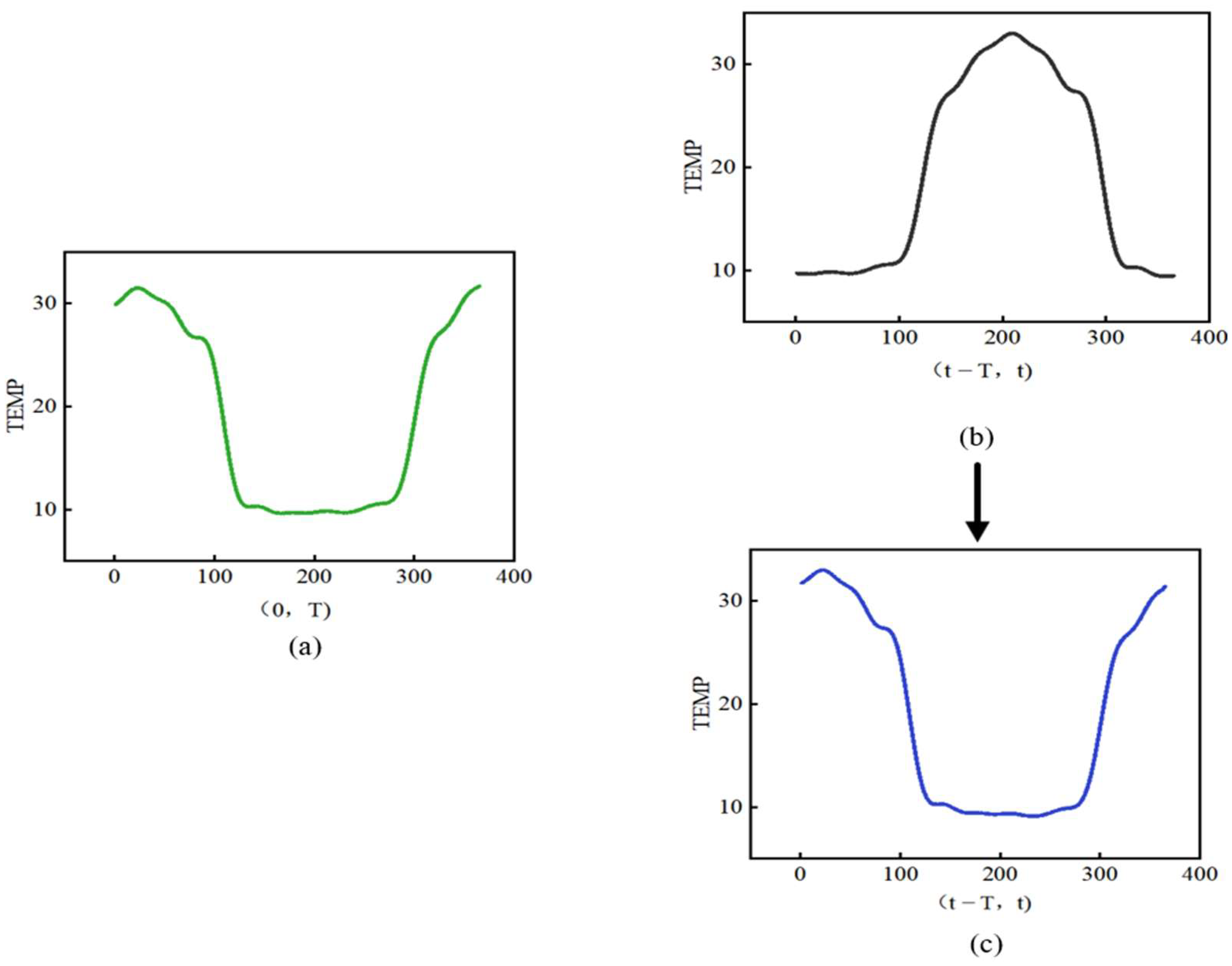
For smoothed data, it is straightforward to calculate the SOC between the health state benchmark data and the real-time operational data. However, for data with complex cyclical changes, the real-time operational data need to be rearranged. To maintain a consistent trend between the change in data for the most recent full cycle where the assessment point data are located and the change in health status benchmark data, the method of operation is to fill in the corresponding position state data of the last orbital cycle by replacing them with real-time in-orbit operational data. The Pearson coefficient is then calculated to analyze the similarity of change. The effect is shown in Figure 3.

The DDD before and after rearrangement are the same as those calculated for the ideal health benchmark data. However, the variation in SOC is significant. This difference is not due to the poor operational status of the data, but mainly to the different points in time of the assessment. Such effects can be eliminated by rearranging and analyzing the differences between the operational and benchmark data changes.

3.3. Single Parametric Health Assessment Based on HDDD and SOC

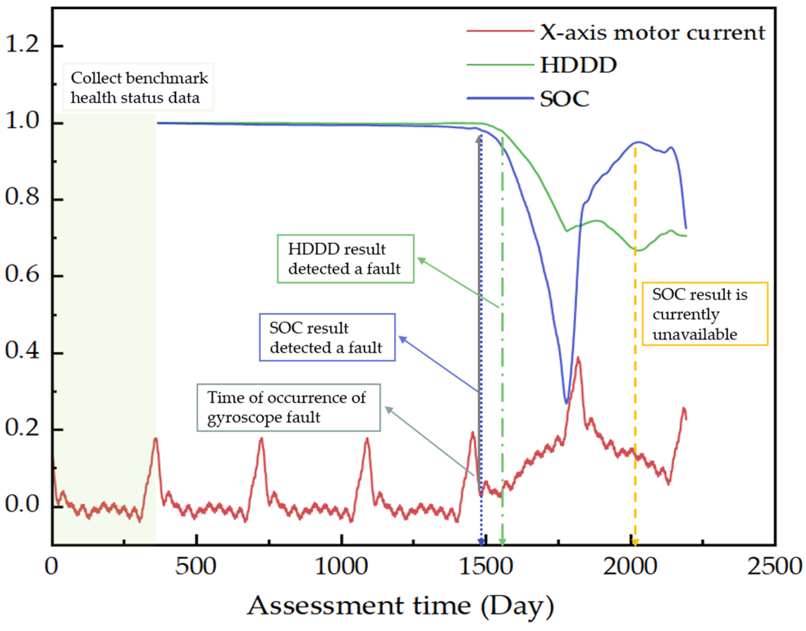
The motor current is an important health characteristic parameter of the gyroscope component. Taking the preprocessed X-axis motor current of a gyroscope component with a fault as an example, the single-parameter health state description method presented in this paper is shown in Figure 4. During in-orbit health assessment, the benchmark data of the current health status should be collected first. Following data collection, the HDDD and SOC of the current data should be calculated separately. From the start of the assessment until day 1500, both HDDD and SOC exhibited only a slow and slight downward trend. From Figure 4, it can be seen that a fault occurred around day 1500, when the current data became abnormal. Soon after, the SOC result decreased significantly, indicating an abnormal health status of the component, which reflects the advantage of SOC in detecting changes in component status in the early stage. After a period of time, the HDDD result also decreased to a certain extent, indicating a change in the component status. However, after day 1760, due to the increasing similarity between the real-time current operating data and the baseline data, the SOC result showed an upward trend, and temporarily became invalid on day 2000. At this point, the HDDD perfectly compensated for the deficiency of the SOC in assessing data changes when the data amplitude was different, but the similarity was high. In summary, the DDD and SOC analyze the health status of parameters from different perspectives, complementing each other. Combining DDD and SOC can accurately, reasonably, and comprehensively describe the health status changes of a single parameter.

4. Multi-Parameter Component Evaluation Model and Verification Method

4.1. Establishment of Multi-Parameter Component Evaluation Model

The objective of the weighting model is to accurately and scientifically reflect the importance of the different parameters. The main health characteristic parameters selected through work mechanism analysis and expert experience can exclude the influence of irrelevant parameters. Irrelevant parameters mainly include parameters that cannot significantly reflect the changes of component health status, flag bits, etc. In this case, the use of the subjective weighting method cannot avoid the influence of strong subjectivity. The objective weighting method relies solely on the data and can yield more reasonable results. The entropy method and the CRITIC method complement each other, and the combination of the two can yield more reasonable weight results.

4.1.1. CRITIC Method

The CRITIC (Criteria Importance through Intercriteria Correlation) method is an objective weighting method. The idea is to compare the intensity and conflicting indicators [44]. The intensity of the comparison is expressed using the standard deviation, with a higher standard deviation of the data indicating greater fluctuations and a higher weighting. Conflict is expressed using the correlation coefficient. The higher the value of the correlation coefficient between parameters, the less conflicting it is. Therefore, the more information that is repeated in the evaluation content, the lower the weighting will be. For multi-parameter comprehensive evaluation problems, the CRITIC method can eliminate the influence of some highly correlated parameters, reducing the overlap of information on the parameters. This is more conducive to obtaining credible evaluation results [45].

The steps to model the configuration of the parameter weights are as follows.

(1)

Normalization of data for each parametric indicator.

Positive indicator:

$${\mathrm{x}}_{\mathrm{ij}}^{\prime }=\frac{{\mathrm{X}}_{\mathrm{ij}}-{\min (\mathrm{X}}_{1\mathrm{j}},\cdots {,\mathrm{X}}_{\mathrm{nj}})}{{\max (\mathrm{X}}_{1\mathrm{j}},\cdots {,\mathrm{X}}_{\mathrm{nj}})-{\min (\mathrm{X}}_{1\mathrm{j}},\cdots {,\mathrm{X}}_{\mathrm{nj}})}$$

(11)

Negative indicator:

$${\mathrm{x}}_{\mathrm{ij}}^{\prime }=\frac{{\max (\mathrm{X}}_{1\mathrm{j}},\cdots {,\mathrm{X}}_{\mathrm{nj}})-{\mathrm{X}}_{\mathrm{ij}}}{{\max (\mathrm{X}}_{1\mathrm{j}},\cdots {,\mathrm{X}}_{\mathrm{nj}})-{\min (\mathrm{X}}_{1\mathrm{j}},\cdots {,\mathrm{X}}_{\mathrm{nj}})}$$

(12)

(2)

Calculation of indicator variability.

$$\{\begin{array}{c}\overline{{\mathrm{x}}_{\mathrm{j}}}=\frac{1}{\mathrm{n}}{\displaystyle \sum _{\mathrm{i}=1}^{\mathrm{n}}}{\mathrm{x}}_{\mathrm{ij}}\\ {\mathrm{S}}_{\mathrm{j}}=\sqrt{\frac{{{\displaystyle \sum }}_{\mathrm{i}=1}^{\mathrm{n}}{{(\mathrm{x}}_{\mathrm{ij}}-\overline{{\mathrm{x}}_{\mathrm{j}}})}^2}{\mathrm{n}-1}}\end{array}$$

(13)

In Equation (13), ${\mathrm{S}}_{\mathrm{j}}$ denotes the standard deviation of the jth parametric indicator.

(3)

Indicator conflict calculation.

$${\mathrm{R}}_{\mathrm{j}}={\displaystyle \sum }_{\mathrm{i}=1}^{\mathrm{p}}\left(1-{\mathrm{r}}_{\mathrm{ij}}\right)$$

(14)

In Equation (14), ${\mathrm{r}}_{\mathrm{ij}}$ denotes the correlation coefficient between the ith parametric indicator and the jth parametric indicator.

(4)

Calculation of information volume.

The greater the amount of information reflected by a parameter, the greater the role of that parameter in the overall picture and the greater the weight should be given.

$${\mathrm{C}}_{\mathrm{j}}{ = \mathrm{S}}_{\mathrm{j}}{\displaystyle \sum }_{\mathrm{i}=1}^{\mathrm{p}}\left(1-{\mathrm{r}}_{\mathrm{ij}}\right){=\mathrm{S}}_{\mathrm{j}}{ \times \mathrm{R}}_{\mathrm{j}}$$

(15)

(5)

Determining weights.

Based on the above analysis, the objective weight for parametric indicator j is:

$${\mathrm{W}}_{\mathrm{j}}=\frac{{\mathrm{C}}_{\mathrm{j}}}{{{\displaystyle \sum }}_{\mathrm{j}=1}^{\mathrm{p}}{\mathrm{C}}_{\mathrm{j}}}$$

(16)

4.1.2. Entropy Method

Compared with subjective assignment methods such as Delphi and hierarchical analysis, the entropy method is more objective and better able to interpret the results [46]. It uses the variability between information to assign weights and avoid bias caused by human factors.

The steps to build an entropy-weighted configuration model of the parametric capacity indicator system are as follows [47,48].

(1)

Determining the objective function.

Construct an objective function for the objective weighting model of a performance indicator based on the criterion of great entropy of information entropy theory:

$$\max \mathrm{Z}=-{\displaystyle \sum }_{\mathrm{j}=1}^{\mathrm{m}}{\mathrm{w}}_{\mathrm{ij}}{\mathrm{lnw}}_{\mathrm{ij}}$$

(17)

In Equation (17), ${\mathrm{w}}_{\mathrm{ij}}$ denotes the jth performance indicator weight for the ith capability. There are a total of m performance indicators describing that capability.

(2)

Determining constraints.

First, the weight sum is 0. Second, the weight value is greater than 0. Third, the ability of different covariate degradation amounts to reflect the overall degradation trend ${\mathrm{g}}_{\mathrm{i}}$ is calculated, and constitutes a parametric capacity variability constraint. It is also necessary to standardize and make dimensionless the parametric indicators here.

(3)

Constructing an entropic configuration model of the capacity indicator system.

Based on the abovementioned objective function and constraints, the following objective planning is established to solve for the objective weights of the performance indicators for the ith capability.

$$\mathrm{s}. \mathrm{t}.\{\begin{array}{c}{\displaystyle \sum _{\mathrm{j}=1}^{\mathrm{m}}}{\mathrm{w}}_{\mathrm{ij}}=1\\ {\mathrm{w}}_{\mathrm{ij}} > 0\\ {\displaystyle \sum _{\mathrm{j}=1}^{\mathrm{m}}}{\mathrm{w}}_{\mathrm{ij}}{\mathrm{g}}_{\mathrm{ij}}^{{\mathrm{k}}_1} < \cdots { < \mathrm{w}}_{\mathrm{ij}}{\mathrm{g}}_{\mathrm{ij}}^{{\mathrm{k}}_2}\end{array}$$

(18)

Analyzing the objective function, the Hessian matrix of the objective function is as follows:

$$\mathrm{H} =\left[\begin{array}{ccc}\frac{{\partial }^2\mathrm{Z}}{\partial {\mathrm{w}}_1^2}& \cdots & \frac{{\partial }^2\mathrm{Z}}{\partial {\mathrm{w}}_1{\mathrm{w}}_{\mathrm{m}}}\\ ⋮& \ddots & ⋮\\ \frac{{\partial }^2\mathrm{Z}}{\partial {\mathrm{w}}_1{\mathrm{w}}_{\mathrm{m}}}& \cdots & \frac{{\partial }^2\mathrm{Z}}{\partial {\mathrm{w}}_{\mathrm{m}}^2}\end{array}\right]=\left[\begin{array}{ccc}\frac{1}{{\mathrm{w}}_1}& & \\ & \ddots & \\ & & \frac{1}{{\mathrm{w}}_{\mathrm{m}}}\end{array}\right]$$

(19)

Since ${\mathrm{w}}_{\mathrm{i}}$ > 0, then |H| > 0. The objective function is convex and the constraints are linear, so it is a convex set. Therefore, the weight allocation model is a convex programming problem on a convex set, and then there must be a unique optimal solution. This leads to the optimal weight assignment of the covariates.

The weights ${\mathrm{w}}_{{\mathsf{\xi }}_{\mathrm{i}}1}$ and ${\mathrm{w}}_{{\mathsf{\xi }}_{\mathrm{i}}2}$ are calculated for each covariate under the CRITIC method and the entropy weight method, respectively. The formula for calculating the combined weight of the covariates is shown in Equation (20):

$${\mathrm{w}}_{{\mathsf{\xi }}_{\mathrm{i}}}=\frac{1}{2}{(\mathrm{w}}_{{\mathsf{\xi }}_{\mathrm{i}}1}{ + \mathrm{w}}_{{\mathsf{\xi }}_{\mathrm{i}}2})$$

(20)

Based on this, a multi-parameter component health assessment model can be established, as shown in Equation (21):

$${\mathrm{f}}_{\mathrm{i}}{\left(\mathsf{\xi }\right)=\mathrm{w}}_{{\mathsf{\xi }}_1}{\mathrm{f}}_{\mathrm{i}}{(\mathsf{\xi }}_1{) + \mathrm{w}}_{{\mathsf{\xi }}_2}{\mathrm{f}}_{\mathrm{i}}{(\mathsf{\xi }}_2) + \cdots { + \mathrm{w}}_{{\mathsf{\xi }}_{\mathrm{n}}}{\mathrm{f}}_{\mathrm{i}}{(\mathsf{\xi }}_{\mathrm{n}})$$

(21)

When i = 1, it represents the component DDD model, and when i = 2, it represents the component SOC model. Additionally, the model can be utilized to calculate the component’s HDDD and DSOC. The model’s corresponding thresholds for different health states were determined through testing with historical data from similar satellites. Once the ideal health state benchmark data for the component are collected, real-time health assessment of the component can be carried out in orbit.

As can be seen from the above-shown analysis, the second prerequisite for the application of this method is that a relatively sufficient sample set of component data is available. This facilitates the testing of algorithms to determine reasonable thresholds for different health status levels.

4.2. Verification of Component Health State Variation Trends Based on Empirical Mode Decomposition

The accuracy and validity of the method can be verified by comparing and analyzing the variation trends extracted from the component DDD, the differences in the similarity of operational data changes (DSOC), and the original data after preprocessing. The current mainstream trend extraction algorithms such as low-pass filtering, least squares, and mean slope methods all require a pre-determined type of trend term for the parametric data [49]. Yet there are so many satellite component parameters that it is impossible to determine the trend of the parameters in advance. The Empirical Mode Decomposition (EMD) algorithm is adaptive and does not require the type of change in the trend term to be determined in advance. This makes it very suitable for trend extraction and comparative analysis [50,51].

The key to the EMD is modal decomposition. The complex data series is decomposed into a finite number of intrinsic mode functions (IMF) and a residual r(t), which is the underlying trend term. The method can be smoothed to handle non-linear, non-smooth data. The EMD method is essentially a way of decomposing the data by the characteristic time scale of the data to ‘filter’ out the eigenmodal function components. The original data series can be expressed as a sum of n IMFs and a residual $\mathrm{r}\left(\mathrm{t}\right)$, as shown in Equation (22):

$$\mathrm{X}\left(\mathrm{t}\right)={\displaystyle \sum }_{\mathrm{i}=1}^{\mathrm{n}}{\mathrm{IMF}}_{\mathrm{i}}\left(\mathrm{t}\right) + \mathrm{r}\left(\mathrm{t}\right)$$

(22)

The stopping condition for the EMD is that the residual $\mathrm{r}\left(\mathrm{t}\right)$ is a monotonic function, so that it is the trend term of the original data series. Therefore, the residuals obtained from the EMD method can be used to efficiently and accurately extract the trends from the data without providing any a priori basis functions.

As the trend term extracted by the EMD algorithm reflects the trend of the overall data, DDD and DSOC can also reflect the degree of deviation from the overall data. Therefore, the EMD algorithm can be employed to extract the change trend of preprocessed raw data, DDD, and DSOC. The validity and accuracy of the method can be verified by calculating the similarity of the three trend lines and analyzing the correlation of changes.

5. Experiment and Verification

5.1. Benchmarking Based on Indicators

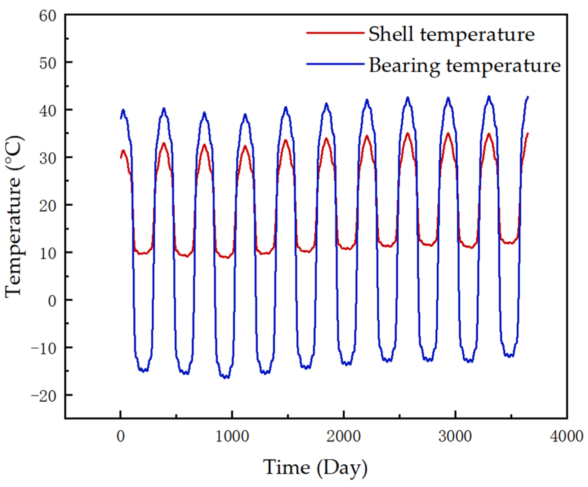
A solar sail component was used as an example to validate the health assessment method described in this paper. The solar sail is a key component of the satellite’s energy system and temperature data best reflect trends in the component’s health status. Two parameters, bearing temperature and shell temperature, were selected for the south solar sail. The sources of the data were telemetry data from a satellite. The two-parametric-decade-run data after preprocessing are shown in Figure 5.

The initial phase of the component run data is more stable. The benchmark is quantified by the variance, standard deviation, and data extreme difference for different cycle quantities of data. The indicators are calculated as shown in

Table 1. Calculation of health benchmark indicators.

Parameter	Indicator	First Cycle	First Two Cycles	First Three Cycles
Shell temperature	Variance	81.0312	85.5062	86.9454
	Standard deviation	9.0141	9.2533	9.3287
	Data extreme difference	22.0052	23.8856	24.1952
Bearing temperature	Variance	549.4529	553.0955	554.9104
	Standard deviation	23.4726	23.5341	23.5673
	Data extreme difference	55.1515	55.9404	56.7974

.

Based on the results of the indicator calculations, it can be found that when the benchmark data are taken as the first full cycle data, all three indicators are the smallest. This indicates the most stable operating data and the best operating condition of the components. Hence, the first-cycle operating data are the most suitable as the ideal health benchmark data.

It is important to note that in order to avoid calculation errors caused by the different magnitudes of parameters, it is necessary to standardize different parameter benchmarks to the same amplitude after collecting the benchmark data.

5.2. Establishment of a Solar Sail Health Assessment Model

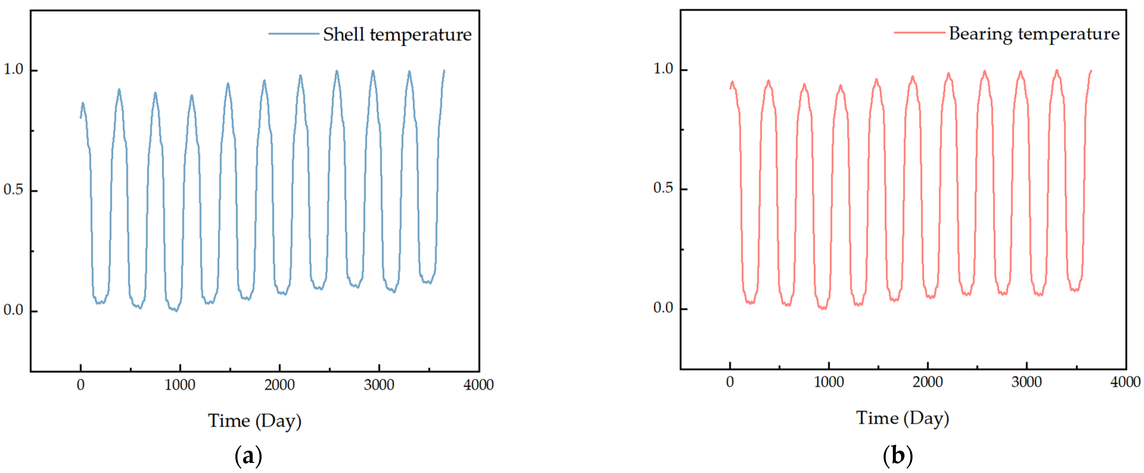
The full life cycle shell and bearing temperature data for a stable operating solar sail were normalized positively and the results are shown in Figure 6. The parameter weights were calculated by the entropy weight method and CRITIC method, and the mean value was taken as the final weight. The results are shown in

Table 2. Results of the calculation of the parameter weights.

	Weighting of Shell Temperature	Weighting of Bearing Temperature
CRITIC method	0.4758	0.5242
Entropy method	0.4883	0.5117
Combined weighting	0.4821	0.5179

.

With a combined shell temperature weight of 0.4821 and a combined bearing temperature weight of 0.5179, the evaluation model is shown in Equation (23):

$$\mathrm{f}\left(\mathsf{\xi }\right)=0.4821{\mathrm{f}(\mathsf{\xi }}_1) + 0.5179{\mathrm{f}(\mathsf{\xi }}_2)$$

(23)

5.3. Solar Sail Health Status Assessment

Solar sail temperature data have high stability requirements. After testing a large number of historical data, 0.95, 0.9, and 0.85 were used as the thresholds for the “Excellent”, “Good”, and “Qualified” status levels based on HDDD, respectively. The cycle variation data should ideally be perfectly positively linearly correlated, i.e., p = 1, and in this case, T = 365, so the sample size is richer. In addition, because of the high reliability requirements of the components, the conventional Pearson correlation coefficient thresholds cannot be used as a basis for the health status classification. Therefore, 0.99, 0.98, and 0.97 were chosen as the thresholds for the “Excellent”, “Good”, and “Qualified” status levels based on SOC, respectively. “Excellent” means that the component is in excellent operating condition and can perform all tasks stably. “Good” means that the component is in good operating condition and can perform most tasks. “Qualified” means that the component is in average operating condition and can only perform some tasks with low performance requirements. A result below the “Qualified” threshold is considered a component fault. It should be noted that there should be a difference in the selection of thresholds for components with high precision requirements and those with low performance requirements.

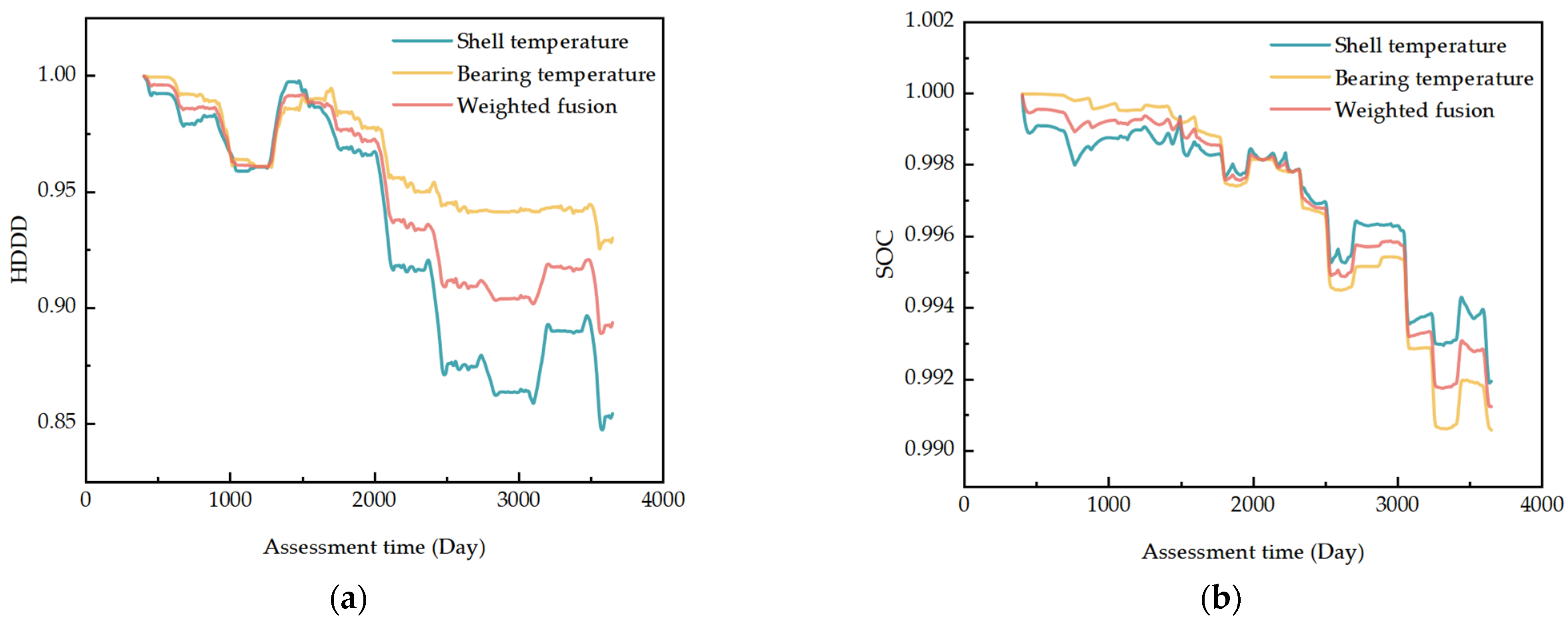
According to the benchmark determined by the index calculation, HDDD and SOC were calculated separately for shell temperature data and bearing temperature data. The results are shown in Figure 7.

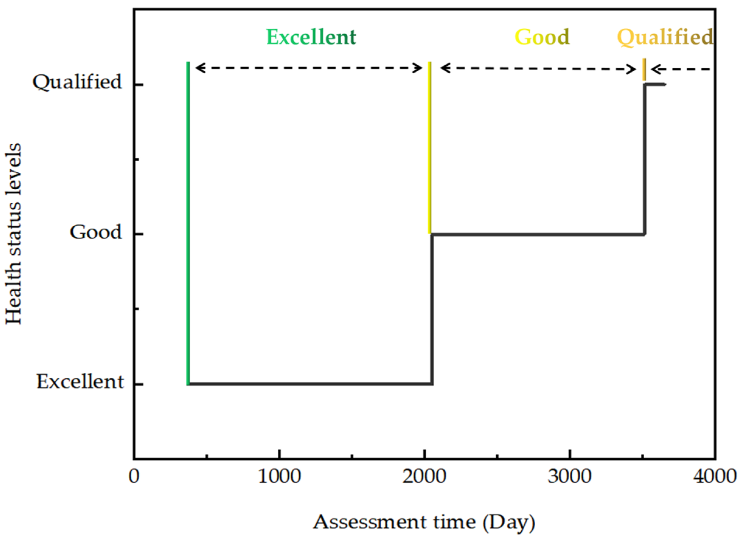
The original data showed a downward and then an upward trend, and the fourth-cycle data were most similar to the benchmark data distribution. Thus, the health of the data distribution showed a significant upward trend in the fourth cycle period. This indicates that the MMD algorithm is able to accurately sense changes in the data distribution, consistent with the actual situation. As the MMD is mainly influenced by the bottom region where the data are more predominant in the calculation of this example data, the health of the component data changes more when it is run to that stage. At the same time, the data selected are stable operational data without faults and abnormalities. Therefore, the similarity results are good and show an approximate monotonic downward trend. It can also be seen from the calculations that the weighted data distribution health indicator HDDD and the SOC trend more smoothly and more closely align with the actual component performance trends. The variation in component status levels in the example is mainly influenced by DDD. The variation in health status levels is shown in Figure 8.

5.4. Verification of Component Health State Variation Trends

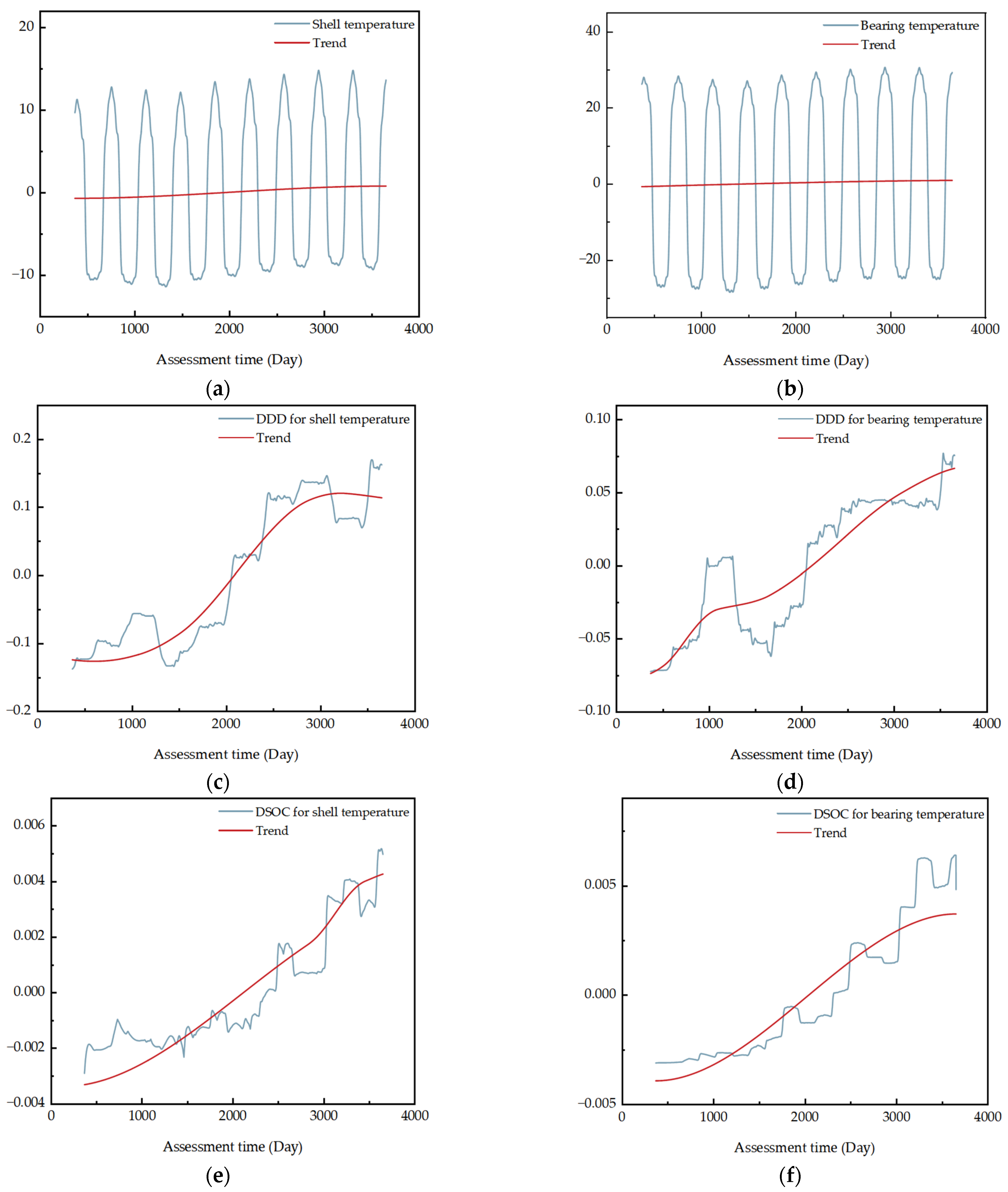
Based on the principle of the algorithm, the data were first zeroed to the mean value separately. The trends in the original data, the results of the DDD calculations, and the results of DSOC were then extracted. The results are shown in Figure 9.

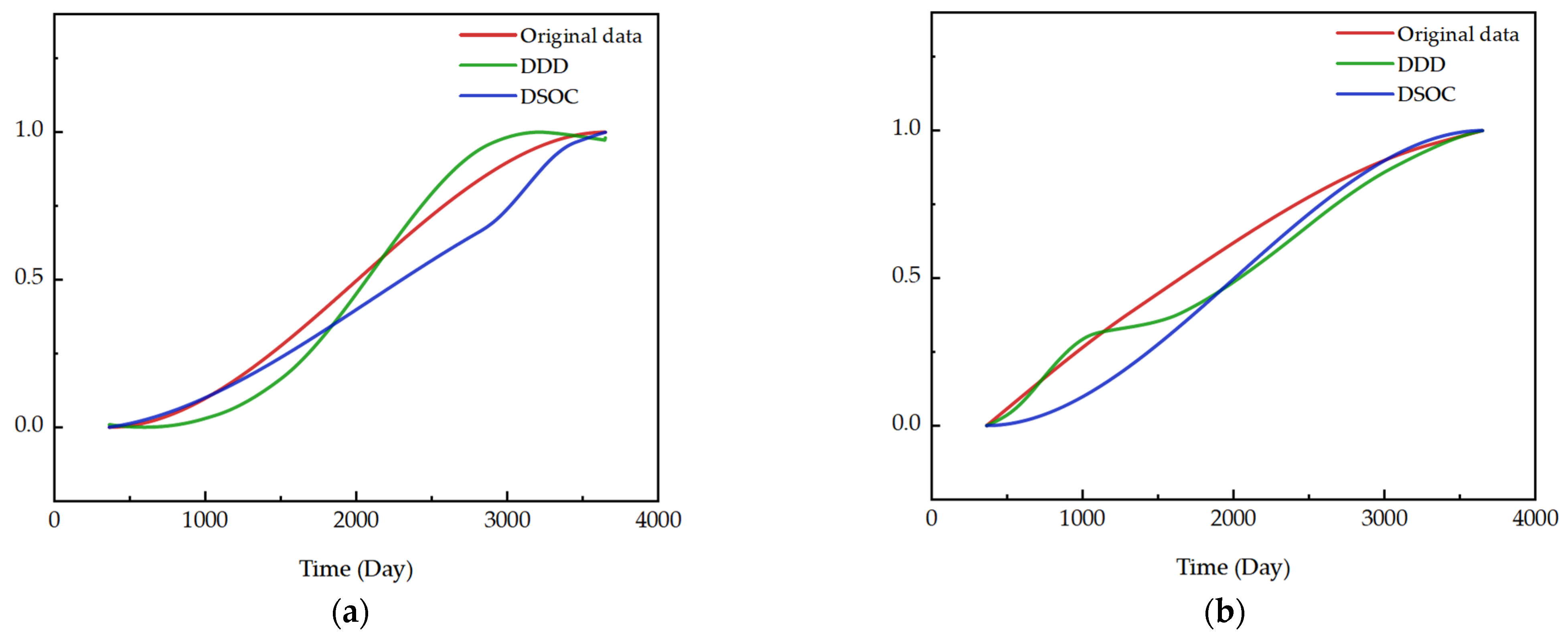
The normalized comparison plots of original data trends after preprocessing, DDD trends, and DSOC trends of the two parameters’ data are shown in Figure 10. The reason for the differences in the details of trend changes is that different algorithms have different principles for describing data changes.

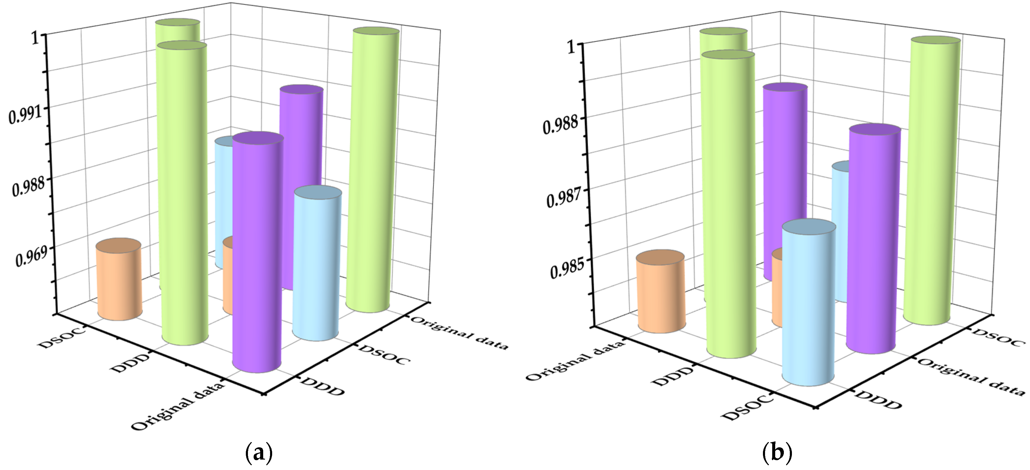
The Pearson correlation coefficient was used to calculate the trend change correlation and the results are shown in Figure 11.

From the calculation results, it can be observed that the original data trend, the trend of DDD, and the trend of DSOC were highly correlated. This verifies the accuracy and validity of the health assessment method utilized in this paper.

6. Conclusions

This study presented a method for assessing the health of key satellite components based on the characteristics of multiparameter data distribution. Determining the health benchmark data through indicators and setting reasonable thresholds enables comprehensive multi-parameter health assessment using only short-term operational data. As a result, this method is able to describe changes in component health status through real-time component operational data. Compared with existing methods such as extracting long-term data trends to build component performance degradation models and neural networks, the method presented in this paper is advanced in three ways. (1) The method has lower data requirements, with no need for long-term operational data to extract trends and the ability to use only short-term data for real-time health assessments. (2) The trend extraction algorithm is only able to extract monotonic trends in the long-term data as a whole. This method provides a more accurate and reasonable description of the details of the changes in the health status of the components at different stages. (3) The assessment results are calculated from the analysis of the component operation data. This avoids the errors that arise from modeling and analyzing cyclical variation data with neural network models. The results showed that the component health assessment method presented in this paper is highly valid and accurate. In addition, health assessment is a research technique from components to systems, and future research will focus on system health assessment based on this paper.

References

- Mukhachev, P.A.; Sadretdinov, T.R.; Pritykin, D.A.; Ivanov, A.B.; Solov’ev, S.V. Modern Machine Learning Methods for Telemetry-Based Spacecraft Health Monitoring. Autom. Remote Control 2021, 82, 1293–1320. [Google Scholar] [CrossRef]
- Siyang, L.; Fei, Q.; Zhen, G.; Yuan, Z.; Yizhou, H. LTE-Satellite:Chinese Proposal for Satellite Component of IMT-Advanced System. China Commun. 2013, 10, 47–64. [Google Scholar] [CrossRef]
- Zhong, C.; Xu, Z.; Teng, H.-F. Multi-module satellite component assignment and layout optimization. Appl. Soft Comput. 2019, 75, 148–161. [Google Scholar] [CrossRef]
- Serfontein, Z.; Kingston, J.; Hobbs, S.; Impey, S.A.; Aria, A.I.; Holbrough, I.E.; Beck, J.C. Effects of long-term exposure to the low-earth orbit environment on drag augmentation systems. Acta Astronaut. 2022, 195, 540–546. [Google Scholar] [CrossRef]
- Hassanien, A.E.; Darwish, A.; Abdelghafar, S. Machine learning in telemetry data mining of space mission: Basics, challenging and future directions. Artif. Intell. Rev. 2019, 53, 3201–3230. [Google Scholar] [CrossRef]
- Sadiqa, J.; YungCheol, B. XGBoost-Based Remaining Useful Life Estimation Model with Extended Kalman Particle Filter for Lithium-Ion Batteries. Sensors 2022, 22, 9522. [Google Scholar]
- Zheng, W.; Peng, G.; Xuening, C. Remaining Useful Life Prediction of Wind Turbine Gearbox Bearings with Limited Samples Based on Prior Knowledge and PI-LSTM. Sustainability 2022, 14, 12094. [Google Scholar]
- Minkoo, K.; Sunjae, L.; Ho, K.J.; Sei, Y.C.; Joongsoon, J.; Mekbibe, N.B.; Sangchul, P. Remaining useful life estimation using accelerated degradation test, a gamma process, and the arrhenius model for nuclear power plants. J. Mech. Sci. Technol. 2022, 36, 4905–4912. [Google Scholar]
- Rong, Z.; Yuan, C.; Weiwen, P.; Zhi-Sheng, Y. Bayesian deep-learning for RUL prediction: An active learning perspective. Reliab. Eng. Syst. Saf. 2022, 228, 108758. [Google Scholar]
- Bach, P.D.; Jong-Myon, K. Prognosis of remaining bearing life with vibration signals using a sequential Monte Carlo framework. J. Acoust. Soc. Am. 2019, 146, EL358–EL363. [Google Scholar]
- Mingxian, W.; Hongyan, W.; Langfu, C.; Gang, X.; Xiaoxuan, H.; Qingzhen, Z.; Juan, C. Remaining Useful Life Prediction for Aero-Engines Based on Time-Series Decomposition Modeling and Similarity Comparisons. Aerospace 2022, 9, 609. [Google Scholar]
- Zhang, K.; Jiang, B.; Mao, Z. Incipient Fault Detection for Traction Motors of High-Speed Railways Using an Interval Sliding Mode Observer. IEEE Trans. Intell. Transp. Syst. 2019, 20, 2703–2714. [Google Scholar] [CrossRef]
- Pirmoradi, F.N.; Sassani, F.; Silva, C.W.d. Fault detection and diagnosis in a spacecraft attitude determination system. Acta Astronaut. 2009, 65, 710–729. [Google Scholar] [CrossRef] [Green Version]
- Rahimi, A.; Kumar, K.D.; Alighanbari, H. Fault detection and isolation of control moment gyros for satellite attitude control subsystem. Mech. Syst. Signal Process. 2020, 135, 106419. [Google Scholar] [CrossRef]
- Liu, Y. Discrimination of low- and high-demand modes of safety-instrumented systems based on probability of failure on demand adaptability. Proc. Inst. Mech. Eng. Part O J. Risk Reliab. 2014, 228, 409–418. [Google Scholar] [CrossRef]
- Weihua, L.; Wansheng, Y.; Gang, J.; Junbin, C.; Jipu, L.; Ruyi, H.; Zhuyun, C. Clustering Federated Learning for Bearing Fault Diagnosis in Aerospace Applications with a Self-Attention Mechanism. Aerospace 2022, 9, 516. [Google Scholar]
- Schwabacher, M. A survey of data-driven prognostics. In Proceedings of the Infotech@Aerospace, Arlington, VA, USA, 26 September 2005–29 September 2005. [Google Scholar] [CrossRef] [Green Version]
- Islam, M.S.; Rahimi, A. A Three-Stage Data-Driven Approach for Determining Reaction Wheels’ Remaining Useful Life Using Long Short-Term Memory. Electronics 2021, 10, 2432. [Google Scholar] [CrossRef]
- Huang, W.; Andrada, R.; Borja, D. A Framework of Big Data Driven Remaining Useful Lifetime Prediction of On-Orbit Satellite. In Proceedings of the 2021 Annual Reliability and Maintainability Symposium (RAMS), Tucson, AZ, USA, 24–27 January 2021; pp. 1–7. [Google Scholar]
- Song, Y.; Liu, D.; Yang, C.; Peng, Y. Data-driven hybrid remaining useful life estimation approach for spacecraft lithium-ion battery. Microelectron. Reliab. 2017, 75, 142–153. [Google Scholar] [CrossRef]
- Islam, M.S.; Rahimi, A. Use of a data-driven approach for time series prediction in fault prognosis of satellite reaction wheel. In Proceedings of the 2020 IEEE International Conference on Systems, Man, and Cybernetics (SMC), Toronto, ON, Canada, 11–14 October 2020; pp. 3624–3628. [Google Scholar]
- Suo, M.; Zhu, B.; An, R.; Sun, H.; Xu, S.; Yu, Z. Data-driven fault diagnosis of satellite power system using fuzzy Bayes risk and SVM. Aerosp. Sci. Technol. 2019, 84, 1092–1105. [Google Scholar] [CrossRef]
- Varvani Farahani, H.; Rahimi, A. Data-Driven Fault Diagnosis for Satellite Control Moment Gyro Assembly with Multiple In-Phase Faults. Electronics 2021, 10, 1537. [Google Scholar] [CrossRef]
- Chen, H.; Chai, Z.; Dogru, O.; Jiang, B.; Huang, B. Data-driven designs of fault detection systems via neural network-aided learning. IEEE Trans. Neural Netw. Learn. Syst. 2021, 33, 5694–5705. [Google Scholar] [CrossRef] [PubMed]
- Chen, H.; Jiang, B.; Ding, S.X.; Lu, N.; Chen, W. Probability-Relevant Incipient Fault Detection and Diagnosis Methodology with Applications to Electric Drive Systems. IEEE Trans. Control Syst. Technol. 2019, 27, 2766–2773. [Google Scholar] [CrossRef]
- Tsui, K.L.; Chen, N.; Zhou, Q.; Hai, Y.; Wang, W. Prognostics and health management: A review on data driven approaches. Math. Probl. Eng. 2015, 2015, 1–17. [Google Scholar] [CrossRef] [Green Version]
- Jing, L.; Xudan, Z. Neural Network Model Design for Landscape Ecological Planning Assessment Based on Hierarchical Analysis. Comput. Intell. Neurosci. 2022, 2022, 192622. [Google Scholar]
- Rahbar, A.; Vadiati, M.; Talkhabi, M.; Nadiri, A.A.; Nakhaei, M.; Rahimian, M. A hydrogeochemical analysis of groundwater using hierarchical clustering analysis and fuzzy C -mean clustering methods in Arak plain, Iran. Environ. Earth Sci. 2020, 79, 1–17. [Google Scholar] [CrossRef]
- Wang, T.; Ting, W.; Kun, C.; Kanjun, Z.; Zheng’an, D.; Jun, L.; Di, D. Mixed Weibull distribution model of DC protection system based on entropy weight method. J. Phys. Conf. Ser. 2020, 1633, 012098. [Google Scholar] [CrossRef]
- Žižović, M.; Miljković, B.; Marinković, D. Objective methods for determining criteria weight coefficients: A modification of the CRITIC method. Decision Making: Applications in Management and Engineering 2020, 3, 149–161. [Google Scholar] [CrossRef]
- Han, Z.; Chen, X.; Li, G.; Sun, S. A novel 3D-QSAR model assisted by coefficient of variation method and its application in FQs’ modification. J. Iran. Chem. Soc. 2020, 18, 661–675. [Google Scholar] [CrossRef]
- Alinezhad, A.; Khalili, J.; Alinezhad, A.; Khalili, J. CRITIC method. In New Methods and Applications in Multiple Attribute Decision Making (MADM); Springer: Berlin/Heidelberg, Germany, 2019; pp. 199–203. [Google Scholar]
- Lai, H.; Liao, H. A multi-criteria decision making method based on DNMA and CRITIC with linguistic D numbers for blockchain platform evaluation. Eng. Appl. Artif. Intell. 2021, 101, 104200. [Google Scholar] [CrossRef]
- Zhao, J.; Ji, G.; Tian, Y.; Chen, Y.; Wang, Z. Environmental vulnerability assessment for mainland China based on entropy method. Ecol. Indic. 2018, 91, 410–422. [Google Scholar] [CrossRef]
- Mastroianni, G.; Milovanović, G.V. Interpolation Processes: Basic Theory and Applications; Springer: Berlin/Heidelberg, Germany, 2008. [Google Scholar]
- Jia, X.; Sun, F.; Chen, D. Vein Recognition Algorithm Based on Transfer Nonnegative Matrix Factorization. IEEE Access 2020, 8, 101607–101615. [Google Scholar] [CrossRef]
- Jinghui, T.; Dongying, H.; Lifeng, X.; Peiming, S. Multi-scale deep coupling convolutional neural network with heterogeneous sensor data for intelligent fault diagnosis. J. Intell. Fuzzy Syst. 2021, 41, 2225–2238. [Google Scholar]
- Xue-Yang, Z.; Lang, H.; Xiao-Kang, W.; Jian-Qiang, W.; Peng-Fei, C. Transfer fault diagnosis based on local maximum mean difference and K-means. Comput. Ind. Eng. 2022, 172, 108568. [Google Scholar]
- Pan, S.J.; Tsang, I.W.; Kwok, J.T.; Yang, Q. Domain adaptation via transfer component analysis. IEEE Trans. Neural Netw. 2010, 22, 199–210. [Google Scholar] [CrossRef] [PubMed] [Green Version]
- Gretton, A.; Borgwardt, K.M.; Rasch, M.J.; Schölkopf, B.; Smola, A. A kernel two-sample test. J. Mach. Learn. Res. 2012, 13, 723–773. [Google Scholar]
- Zhou, Z.-H. Machine Learning; Springer Nature: Berlin/Heidelberg, Germany, 2021. [Google Scholar]
- Cohen, I.; Huang, Y.; Chen, J.; Benesty, J.; Benesty, J.; Chen, J.; Huang, Y.; Cohen, I. Pearson correlation coefficient. In Noise Reduction in Speech Processing; Springer: Berlin/Heidelberg, Germany, 2009; pp. 1–4. [Google Scholar]
- Zhou, H.; Deng, Z.; Xia, Y.; Fu, M. A new sampling method in particle filter based on Pearson correlation coefficient. Neurocomputing 2016, 216, 208–215. [Google Scholar] [CrossRef]
- Diakoulaki, D.; Mavrotas, G.; Papayannakis, L. Determining objective weights in multiple criteria problems: The critic method. Comput. Oper. Res. 1995, 22, 763–770. [Google Scholar] [CrossRef]
- Shanshan, Z.; Guiwu, W.; Rui, L.; Xudong, C. Cumulative prospect theory integrated CRITIC and TOPSIS methods for intuitionistic fuzzy multiple attribute group decision making. J. Intell. Fuzzy Syst. 2022, 43, 1–14. [Google Scholar]
- Gong, W.; Wang, N.; Zhang, N.; Han, W.; Qiao, H. Water resistance and a comprehensive evaluation model of magnesium oxychloride cement concrete based on Taguchi and entropy weight method. Constr. Build. Mater. 2020, 260, 119817. [Google Scholar] [CrossRef]
- He, D.; Xu, J.; Chen, X. Information-theoretic-entropy based weight aggregation method in multiple-attribute group decision-making. Entropy 2016, 18, 171. [Google Scholar] [CrossRef] [Green Version]
- Zou, Z.-H.; Yi, Y.; Sun, J.-N. Entropy method for determination of weight of evaluating indicators in fuzzy synthetic evaluation for water quality assessment. J. Environ. Sci. 2006, 18, 1020–1023. [Google Scholar] [CrossRef] [PubMed]
- Cammarota, C.; Curione, M. Trend Extraction in Functional Data of Amplitudes of R and T Waves in Exercise Electrocardiogram. Fluct. Noise Lett. 2017, 16, 1750014. [Google Scholar] [CrossRef]
- Zhiyong, C.; Zhijuan, C.; Hongwei, Z.; Jiajun, X.; Guangyong, Z.; Yi, L.; Yufei, S.; Ling, L.; Xiujuan, Y.; Zhaobing, G. Using Empirical Modal Decomposition to Improve the Daily Milk Yield Prediction of Cows. Wirel. Commun. Mob. Comput. 2022, 2022, 1685841. [Google Scholar]
- ShaoWei, F. An improved method for EMD modal aliasing effect. Vibroengineering PROCEDIA 2020, 35, 76–81. [Google Scholar]
Figure 1.
Online health assessment process for satellite components based on multiparametric data distribution characteristics.
Figure 2.
Selection of characteristic parameters and benchmarking methods.
Figure 3.
Diagram of the effect of real-time operational data rearrangement. (a) is the data change curve for the benchmark (0, T] interval of the parametric health state. (b) is the data change curve for the (t − T, t] interval of the complete operating cycle at time t. (c) is the change curve after rearranging the data for the (t − T, t] interval of the complete operating cycle at time t.
Figure 4.
Single-parameter health state description method.
Figure 5.
Ten years of operational data after preprocessing.
Figure 6.
Positive normalization of (a) shell temperature and (b) bearing temperature.
Figure 7.
Calculation results of (a) the health degree of data distribution deviations (HDDD) and (b) the similarity of operational data changes (SOC).
Figure 8.
Chart of component health status level changes.
Figure 9.
Trend extraction based on empirical mode decomposition algorithm. (a) Extraction of the trend in shell temperature data. (b) Extraction of trend in bearing temperature data. (c) Extraction of the trend in data distribution deviations (DDD) of shell temperature data. (d) Extraction of the trend in data distribution deviations (DDD) of bearing temperature data. (e) Extraction of the trend in differences in the similarity of operational data changes (DSOC) of shell temperature data. (f) Extraction of the trend in differences in the similarity of operational data changes (DSOC) of bearing temperature data.
Figure 10.
Comparison of three trends in (a) shell temperature and (b) bearing temperature after positive normalization.
Figure 11.
Correlation analysis of the three trends in (a) shell temperature and (b) bearing temperature.