Safety and Efficiency Evaluation Model for Converging Operation of Aircraft and Vehicles

Abstract

To explore the mixed traffic characteristics of vehicles and aircraft on the airport surface and solve the problem of real-time conflict detection at key intersections. According to the actual taxiing procedures and airport control rules in China, this paper focus on abstracting the mixed motion process of aircraft and vehicles in the maneuvering area, defining the convergent cross-safety operation scenario. To quantify the driver’s attention to safety separation and the degree of conservatism in adjusting speed, the vehicle deceleration rate and acceleration rate are defined with α as the exponent. Under the same spacing, the vehicle deceleration rate is directly proportional to α, and α is named the vehicle safety sensitivity. At the same time, the rules of speed change of vehicles and aircraft will be designed, and a convergent operation model of aircraft and vehicles will be proposed. Based on real-time speed and separation dynamic assessment of safety and efficiency under different traffic strategies, the computer simulation results show that vehicle safety sensitivity and deceleration rules determine the sequence of vehicles and aircraft when they are passing through in the short term and can affect the proportion of mixed traffic flow in the long run. The safety probability of vehicles passing the intersection first is negatively correlated with vehicle safety sensitivity, while the safety probability of aircraft passing the intersection first is correlated positively with vehicle safety sensitivity. The efficiency of passing without conflict with mixed traffic has an inverse relationship with vehicle safety sensitivity. When the vehicle safety sensitivity takes the value in the interval [0.4, 0.6], a mixed traffic flow with higher safety and efficiency, better stability, and a balanced ratio of locomotives can be obtained.

1. Introduction

To meet the need for the development of comprehensive transportation, the scale of airport construction in China has been expanding. By the end of 2021, there will be 29 airports with an annual throughput of more than 10 million passengers, accounting for 70.8% of the total passenger transport volume [1]. To ensure smooth aircraft surface operation, many airports surface multiple types of special vehicles and aircraft to run together. For example, it is stipulated that ‘Follow Me’ vehicles guide aircraft taxiing, and patrol vehicles regularly inspect the runway status, etc. However, the complex structure of large airports, more intersections, less training for special vehicle drivers, and the lack of standardization and organization of vehicle operations [2] have led to frequent aircraft-vehicle conflicts, scrapes, and other unsafe events, reaching 57% of the total number of ground accidents at airports [3], so that the safety of vehicle operations has gradually become a key issue in the operation of airport surfaces.

In recent years, related research has focused on 2 directions: special vehicle scheduling optimization and surface operation risk identification. In terms of vehicle scheduling, Braaksma et al. [4] established an optimization model for special vehicle safety services based on the critical path method at Toronto International Airport. Cheung et al. [5] established a vehicle scheduling optimization model intending to maximize vehicle utilization or minimize vehicle idle time and solved it by genetic algorithm. Mao et al. [6] studied airport de-icing services and established a heuristic vehicle scheduling algorithm based on the first come first serve Agent to verify the feasibility of the method. Heng et al. [7] proposed a saving algorithm solution to improve the scheduling equilibrium. Padrón et al. [8] defined a bi-objective optimization algorithm for airport surface vehicle scheduling to minimize pre-operation waiting time and turnaround completion time and evaluated it in two busiest airports in Spain. Zhang et al. [9] developed a tri-objective optimization model by maximizing the task volume, minimizing the operation time, and minimizing the number of operations and gave out a solution. Wang et al. [10] developed a greedy algorithm for the airport refueling vehicle scheduling problem with time window constraints. Zaninotto et al. [11] designed a man-in-the-loop aircraft taxiing optimization strategy considering a trailer tow taxiing scheme to reduce fuel consumption and carbon emissions in taxiing. Liu et al. [12] developed a multi-objective optimization model for ferry vehicle scheduling and solved it with a heuristic algorithm, using Kunming Changshui Airport in China as a prototype. Zhao Zheng et al. [13] constructed a multi-agent discrete simulation model based on a surface operation to improve the synergistic optimization of airport dependency rate and flight regularity. In terms of operational risk management, Sun [14] classified vehicle-aircraft scuffing events and analyzed various types of risk events using the bow-tie diagram (Bow-Tie) technique. Wilke et al. [15] proposed an overall risk assessment framework for airport ground operations that integrates all relevant stakeholders, defining risk indicators and quantification methods. Fei et al. [16] defined safety indicators for electric special vehicles and quantified them using a fuzzy integrated assessment method with improved affiliation functions. Wang et al. [17] used FTA (Fault Tree Analysis) to identify risk factors and used GRA (Gray Relational Analysis) and expert scoring methods to obtain risk values for each factor. Zhao et al. [18] proposed a method to verify the safety integrity level of the system based on the Petri net model and Monte Carlo simulation of the dynamic operation of the tractor-trailer during peak hours. Wang et al. [19] established a surface aircraft damage fault tree and applied the fault Tree analysis-optimal distance solution to construct the prevention and control risk proximity index and evaluate the risk prevention and control status of various airport businesses. Tong [20] conducted a qualitative analysis of operational safety and control service quality after the apron handover and discussed the impact of the ‘Follow Me’ vehicle operation command on control load. Hu et al. [21] distinguished between sleepiness and mental fatigue to study the types and nature of fatigue in existing pilots and vehicle drivers. Liu et al. [22] explored the endogenous and exogenous factors of unmanned special vehicle risk in airport flight areas and established a risk assessment model to judge the weight of each factor and quantify the risk index. Wang et al. [23] proposed a critical conflict point identification method in airport flight areas based on median entropy and take Xianyang International Airport in Xi’an as an example to validate it.

The following characteristics exist in the current research: (1) The research objects are mostly apron-wide operating vehicles, such as food trucks, refueling trucks, de-icing trucks, etc., while less research has been conducted on operating special vehicles in the maneuvering areas (including runways, taxiways, and some apron taxiways). (2) The surface operation safety assessment is mainly based on single aircraft collision risk and multiple aircraft taxiing conflicts, such as predicting runway incursion risk in airport flight area based on GEM or LSTM [24,25,26] or using target detection models to identify key locations such as aircraft fuselage and wingtip to identify scraping risk [27,28,29], or constructing risk assessment models with different situations such as aircraft crossing, opposite, convergence waiting, etc. to calculate dynamic conflicts between aircraft [30,31,32,33]. (3) When studying the surface traffic flow, the vehicles and aircraft are separated, with the aircraft being only a service object without considering their cooperative movement of them. In the actual surface operation, special vehicles such as patrol vehicles and ‘Follow Me’ vehicles will be driven in the maneuvering area, and the aircraft will taxi or be dragged in the maneuver area, not a stationary state. The two co-operations affect each other, which leads to great safety risks. According to the airport field operation rules issued by the Civil Aviation Administration of China (CAAC) [34], the rules for driving and controlling special vehicles in the maneuvering area are different, so the existing results of aircraft operation conflict and aircraft traffic flow conflict detection cannot be directly applied to the study of vehicle-aircraft conflict detection.

To explore the mixed operation characteristics of vehicles and aircraft in the airport maneuvering area and solve the problem of real-time conflict detection at key intersections, this paper aims at the mixed motion process of aircraft and vehicles in the maneuvering area, abstracts the real-time operation and mutual influence process of aircraft and vehicles, defines the safe operation scenario under the convergence trend, and designs the speed change rules of vehicles and aircraft respectively. The paper also simulates the cross-passage process of aircraft and vehicles, and the safe operation probability was evaluated based on the real-time speed and separation of them, and the operation efficiency was quantified to provide solutions for improving the safety level of the maneuvering area and formulating efficient passage strategies at key road intersections.

2. Rules for Separation Establishment between Aircraft and Vehicle

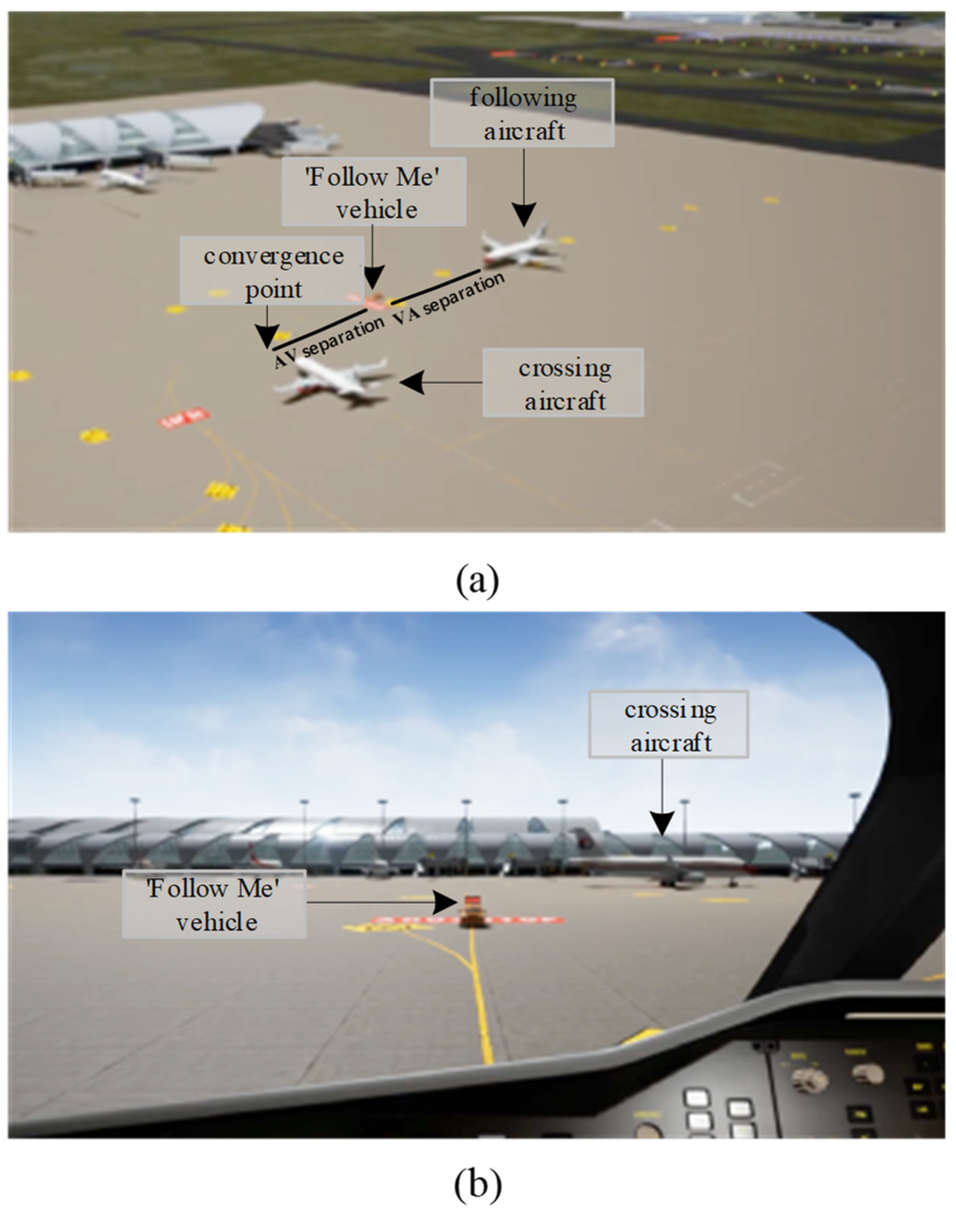
Vehicle and aircraft safety convergence operations are defined as a situation where vehicles and aircraft are traveling in different directions to the same taxiway intersection or key point and passing through the intersection one after the other with a safe separation that is not less than the minimum separation. The Civil Aviation Administration of China stipulates that when the front and rear positions of vehicles and aircraft are different [35,36], they should be equipped with different minimum longitudinal separations. This article refers to the minimum longitudinal separation between the aircraft in front and the vehicle behind as the minimum aircraft-vehicle separation (referred to as AV separation in the following text), and the minimum longitudinal separation between the vehicle in front and the aircraft behind as the minimum vehicle-aircraft separation (referred to as VA separation in the following text).

Figure 1 shows the simulation illustration of different viewpoints before and after the cross-convergence of ‘Follow Me’ vehicles and aircraft. Figure 1a shows the situation before convergence from the controller’s viewpoint, where the ‘Follow Me’ vehicle crosses and converges with an aircraft in front of the side to a convergence point, and the aircraft will pass the intersection first, and the vehicle should slow down or stop in time to keep the minimum locomotive separation with the convergence point. Figure 1b shows the post-convergence situation from the left-seat pilot’s view of the following aircraft. The vehicle slows down or stops, and the following aircraft behind should keep the locomotive separated from the vehicle in time. Due to the small size of the vehicle and the impact of the height of the aircraft cockpit, the pilot can only visually inspect the vehicle if the vehicle is far away from the aircraft, so the minimum VA separation is greater than the minimum AV separation.

3. Aircraft and Vehicle Convergence Safety Assessment Model Set-Up

3.1. An Abstract Description of the Convergence Operation Process

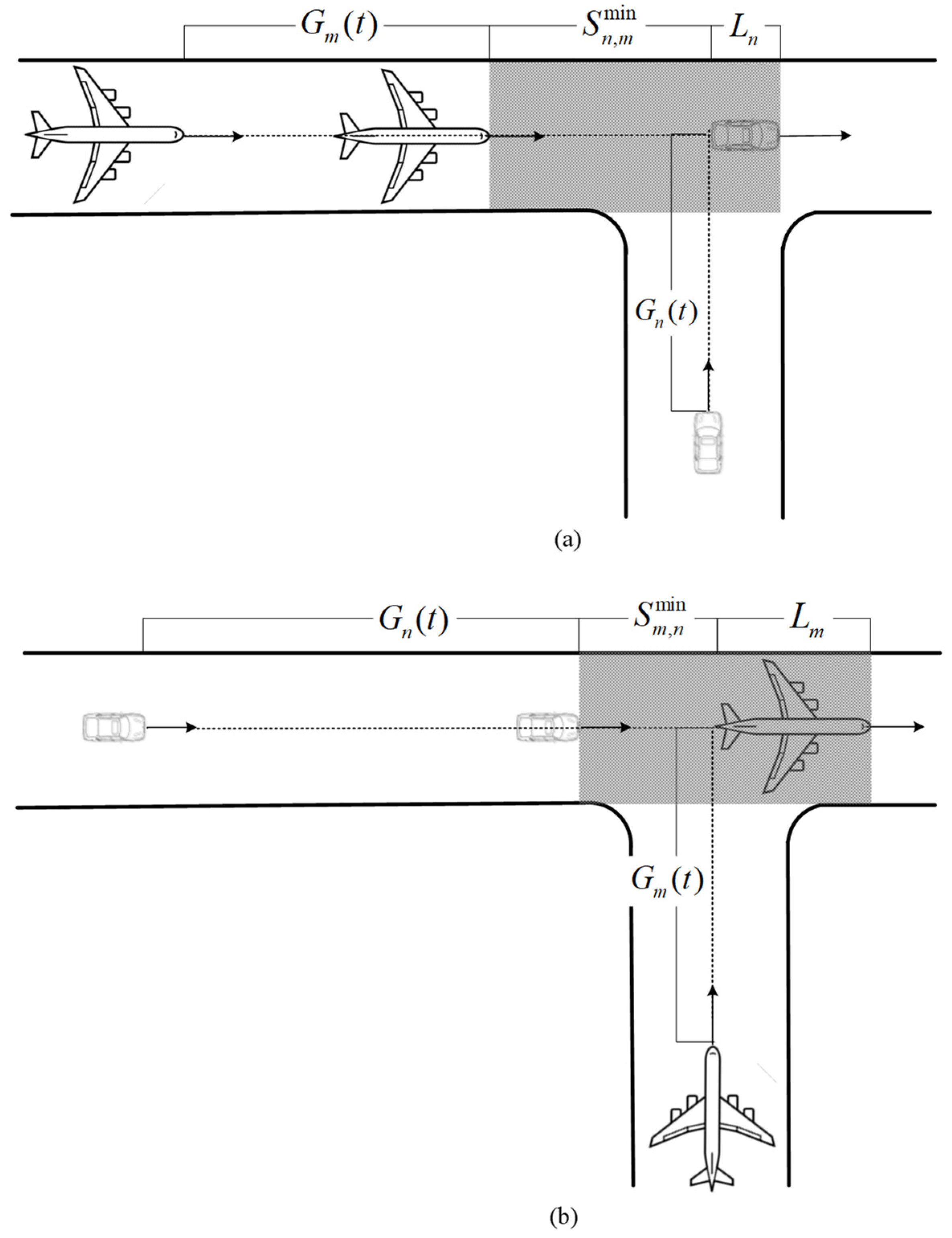
As shown in Figure 2, the taxiway intersection is a T-shaped intersection, and the trajectory of aircraft m and vehicle n crosses at point O. The distance of aircraft m from point O at time t is $G_m(t)$, the velocity is $v_m(t)$, and the length is $l_m$. With vehicle n, at moment t the distance from point O is $G_n(t)$, the velocity is $v_n(t)$, and the length is $l_n$. In Figure 2a, the vehicle crosses the intersection first and $S_{n,m}^{\min }$ is the minimum VA separation. In Figure 2b, the aircraft crosses the intersection first and $S_{m,n}^{\min }$ is the minimum AV separation. The gray rectangle in the figure is defined as the conflict area, for if the vehicle and aircraft are located in this area at the same time, the distance between the two will be less than the minimum safety separation, resulting in conflict. The literature [30,31,32,33] defines the taxiing conflict area between aircraft as a rectangle with a fixed position and area. By comparison with Figure 2, it can be seen that the conflict area and position of the conflict area have changed due to the change of vehicle and aircraft length and minimum safety separation, so the vehicle and aircraft conflict situation is more complicated.

3.2. Vehicle and Aircraft Cross-Motion Regulations

The controller specifies the aircraft’s taxiing path, and the pilot determines the real-time taxiing speed depending on the taxiway arrangement and separation. According to much research [30,31,32,33], the aircraft taxiing speed is equally distributed throughout a narrow range. Set $f_m(t)$ as the probability density function of the velocity of aircraft m at time t. Then there is:

$$f_m(t)=\frac{1}{v_m^{\max }(t)-v_m^{\min }(t)}$$

(1)

The airline advises the captain to employ slower acceleration and deceleration speeds to improve passenger comfort. We have $\Delta {\upsilon }_m$ as speed variance per second. The following requirements should be met by the control provisions for the extreme value of instant taxi speed $v_m^{\max }$:

$$v_m^{\min }(t)\ge \max (0,v_m(t-1)-\Delta {\upsilon }_m)$$

(2)

$$v_m^{\max }(t)\le \min (v_m(t-1)+\Delta {\upsilon }_m,v_m^{\max })$$

(3)

Make the vehicle speed uniformly distributed in a range. $f_m(t)$ is the probability density function of the speed of vehicle n at time t. Then we have:

$$f_n(t)=\frac{1}{v_n^{\max }(t)-v_n^{\min }(t)}$$

(4)

The distance between the aircraft and the vehicle is calculated from the perspective of the vehicle driver and is given as:

$$\Delta d(t)=\left|G_m(t)-G_n(t)\right|$$

(5)

Since relevant studies have been conducted to validate the relationship between complex driver responses, speed estimation, and personality traits [37,38]. In airport field operations, a linear relationship between vehicle-aircraft separation and deceleration has also been defined [39]. However, the linear relationship can only describe ideal motion states such as uniform acceleration and deceleration. Therefore, in this paper, the deceleration rate is replaced by the acceleration and deceleration rates, and the exponential relationship between separation and acceleration and deceleration rates is defined as follows. The vehicle safety sensitivity is defined as $\alpha$, and the rate of increase or decrease of vehicle speed as:

$$r^a(t)=\max (1,{\left(\frac{\Delta d(t-1)}{S_{m,n}^{\min }}\right)}^{\alpha })$$

(6)

$$r^d(t)={\left(\frac{S_{m,n}^{\min }}{\Delta d(t-1)+1}\right)}^{\alpha }$$

(7)

The following conditions should be met by using the control provisions for the vehicle’s maximum speed for $v_n^{\max }$, each moment of speed variance for $\Delta {\upsilon }_n$, and t moment vehicle speed maximum and minimum value:

$$v_n^{\max }(t)\le \min (v_n(t-1)+r^a(t)\Delta {\upsilon }_n,v_n^{\max })$$

(8)

$$v_m^{\min }(t)\ge \max (0,v_n(t-1)-r^d(t)\Delta {\upsilon }_n)$$

(9)

The speed update rule of the vehicle under the impact of aircraft position is described by the equation above. The greater $\alpha$, the more sensitive the vehicle is to the aircraft position. If $\Delta d(t)$ is smaller, the vehicle tends to slow down more at time t. in contrast, if $\Delta d(t)$ is greater, the tendency is for the vehicle to pick up speed at time t.

3.3. Vehicle and Aircraft Cross-Motion Safety Assessment

Set $T_n^{\mathrm{O}}(t)$ and $T_m^{\mathrm{I}}(t)$ as the anticipated times for vehicle n departure and aircraft m entry into the area of conflict at time t respectively, as shown in Figure 2a.

$$T_n^{\mathrm{O}}(t)=\frac{G_n(t)+L_n}{v_n(t)}$$

(10)

$$T_m^{\mathrm{I}}(t)=\frac{G_m(t)-S_{n,m}^{\min }}{v_m(t)}$$

(11)

Under the following circumstances, the aircraft enters the conflict area after the vehicle has left it:

$$T_n^{\mathrm{O}}(t)\le T_m^{\mathrm{I}}(t)\Rightarrow \frac{G_n(t)+L_n}{v_n(t)}\le \frac{G_m(t)-S_{n,m}^{\min }}{v_m(t)}$$

(12)

According to Figure 2b, let the predicted vehicle entry and aircraft departure times from the conflict area at time t be $T_n^{\mathrm{I}}(t)$ and $T_m^{\mathrm{O}}(t)$:

$$T_n^{\mathrm{I}}(t)=\frac{G_n(t)-S_{m,n}^{\min }}{v_n(t)}$$

(13)

$$T_m^{\mathrm{O}}(t)=\frac{G_m(t)+L_m}{v_m(t)}$$

(14)

Under the following circumstances, the vehicle enters the conflict area after the aircraft has left it:

$$T_m^{\mathrm{O}}(t)\le T_n^{\mathrm{I}}(t)\Rightarrow \frac{G_m(t)+L_m}{v_m(t)}\le \frac{G_n(t)-S_{m,n}^{\min }}{v_n(t)}$$

(15)

Equations (12) and (15) should be rewritten as linear functions of velocity that are represented in terms of ${\phi }_n(v_m(t),v_n(t))$ and ${\phi }_m(v_m(t),v_n(t))$.

$${\phi }_n(v_m(t),v_n(t))=v_m(t)-\frac{G_m(t)-S_{n,m}^{\min }}{G_n(t)+L_n}{v}_n(t)$$

(16)

$${\phi }_m(v_m(t),v_n(t))=v_n(t)-\frac{G_n(t)-S_{m,n}^{\min }}{G_m(t)+L_m}{v}_m(t)$$

(17)

Set $P_n(t)$ as the safety probability of the aircraft entering after the vehicle leaves the conflict area at time t, and $P_m(t)$ be the safety probability of the vehicle entering after the aircraft leaves the conflict area at time t.

$$P_n(t)={\displaystyle \iint {\phi }_n(v_m(t),v_n(t))\mathrm{d}{v}_n(t)\mathrm{d}{v}_m(t)}$$

(18)

$$P_m(t)={\displaystyle \iint {\phi }_m(v_m(t),v_n(t))\mathrm{d}{v}_n(t)\mathrm{d}{v}_m(t)}$$

(19)

4. Safety Assessment Simulation Design and Data Analysis

4.1. Simulation Platform Set-Up

The intersection encounter process of an aircraft taxiing and a vehicle traveling, as shown in Figure 2, is simulated from the viewpoints of pilots and vehicle drivers in this paper based on the taxiway configuration. The positions of the vehicle and the aircraft within the observable range and the speed change of the vehicle and aircraft at the next moment during the simulation period T are also dynamically calculated. In this paper, the taxiing speed variation of aircraft at each step is dynamically calculated according to the taxiway configuration within the visual range and the position of the proceeding aircraft from the perspective of pilots. In this way, the taxiing process of aircraft under visual separation within period T can be simulated.

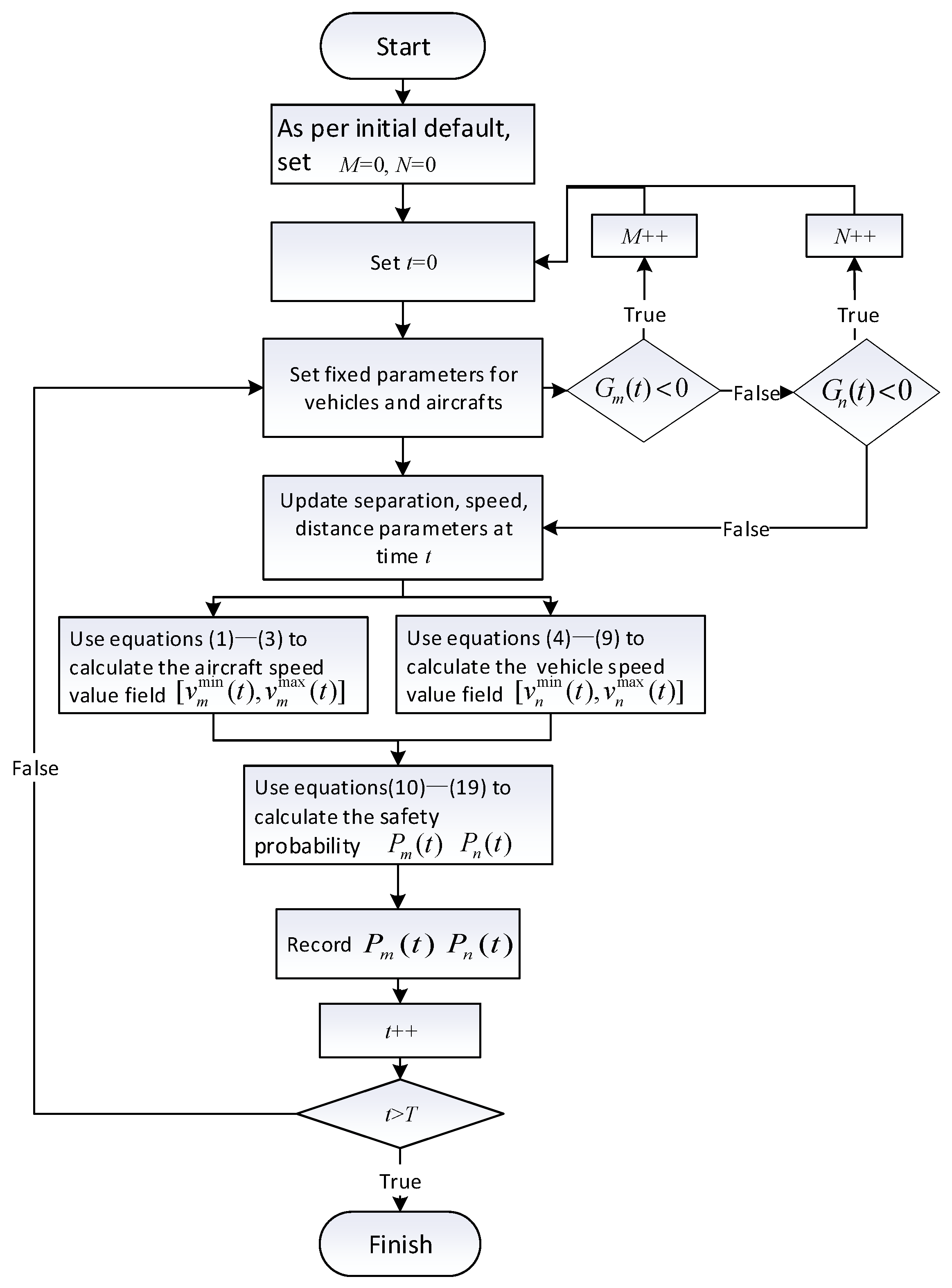
Establish the intersection and taxiway structure as shown in Figure 2, then generate the vehicles and aircraft at the entrance ends of the two taxiways by specific ratio and taxi separation regulations. Finally, carry out speed and position changes by the model rules in this paper. Figure 3 illustrates the specific program flow. Design and implement a simulation program that is programmed to realize the paper’s model for the dynamic simulation of multiple aircraft and vehicles crossover operations, record the position and speed of aircraft and vehicles per second, set the number of aircraft and vehicles that can pass through an intersection without colliding as M and N, and then record the values of M and N in the simulation.

Figure 3 shows the simulation process of dynamically updating aircraft and vehicle velocities and positions and calculating safety probabilities, restarting the simulation, and recording the sorties if the vehicles or aircraft occupy the intersection at the same time. The speed evolution process and safety posture of aircraft and vehicles under the impact of various parameters can be repeatedly simulated by repeating the aforementioned processes.

Set the following parameters with common transport models and special vehicles: $L_m$ = 40 m, $L_n$ = 5 m. The following parameters are initially set for the simulation, $v_m(t_0)=v_n(t_0)$ = 5 m/s, $G_m(t_0)=G_n(t_0)$ = 700 m. Set the following parameters according to the control rules [34,35,36], $S_{n,m}^{\min }$ = 200 m, $S_{m,n}^{\min }$ = 50 m, $v_m^{\max }$ = 13.8 m/s, $v_n^{\max }$ = 12.5 m/s, $\Delta {\upsilon }_n$ = 1.5 m/s.

In the simulation, the following three variables are predetermined: vehicle safety sensitivity $\alpha$, $\alpha \in \{0,0.5,1\}$; aircraft speed variance $\Delta {\upsilon }_m$, $\Delta {\upsilon }_m\in [0.1,0.6]$, the unit of $\Delta {\upsilon }_m$ is m/s, each time increasing by 0.02 m/s; and simulation times $t\in [0,60]$, the unit of t is second, each time increasing by 1 s. The following simulation process will be repeated 500 times to obtain the average value after removing the random influence of the uniform distribution of speed from each simulation’s 3 × 61 × 26 results.

4.2. Safety Assessment in the Case of the Vehicle Passing an Intersection First

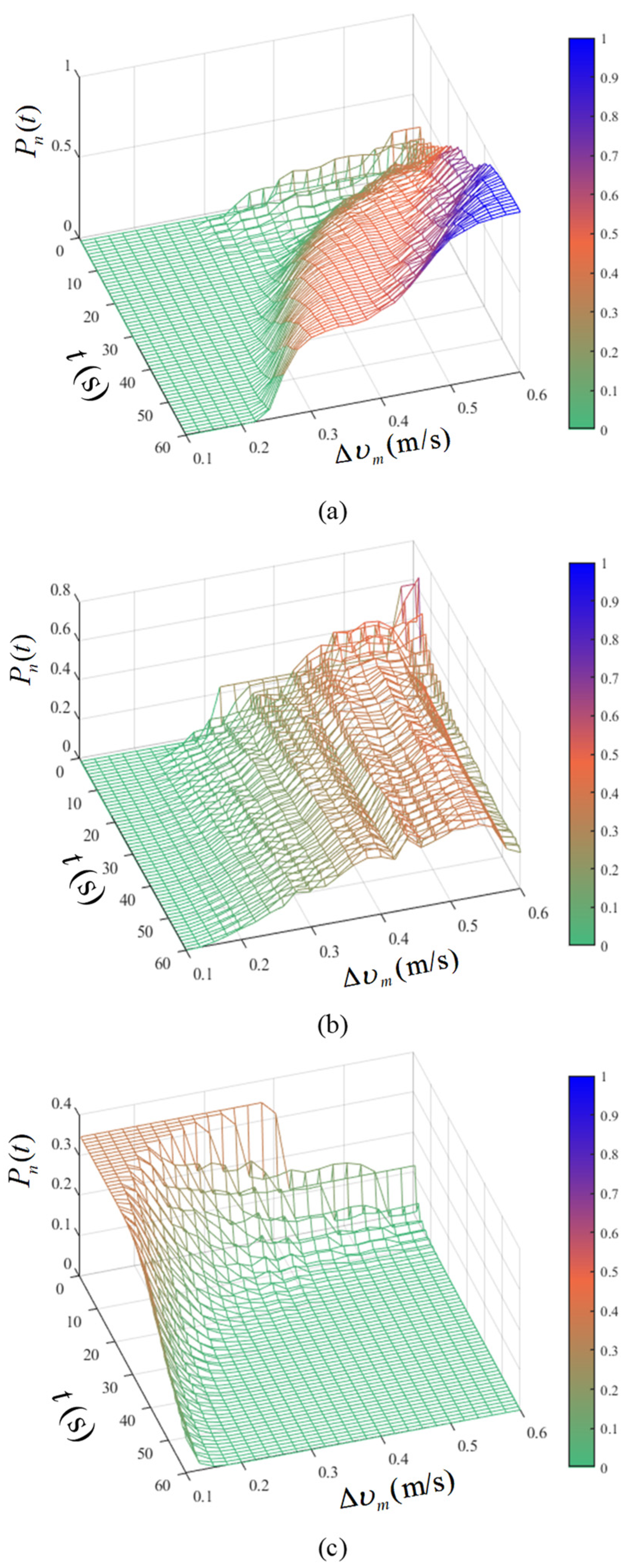
For the scenario where the vehicle crosses the intersection first, as illustrated in Figure 2a, Figure 4 displays the trend of the safety probability $P_n(t)$ with time t, aircraft speed variance $\Delta {\upsilon }_m$, and vehicle sensitivity $\alpha$.

When $\alpha$ = 0, the vehicle operates independently of the aircraft when it follows the prescribed acceleration and deceleration random speed regulation and is not impacted by the aircraft’s position or distance. As shown in Figure 4a, when $\Delta {\upsilon }_m\le 0.2$ m/s, $P_n(t)=0$, and the aircraft speed change are very modest, the vehicle and the aircraft in 60 s cannot pull away from the safe distance of 200 m, and the conflict will occur when the vehicle arrives at the intersection before the aircraft. When $\Delta {\upsilon }_m>0.2$ m/s, $P_n(t)$ is positively associated with both t and $\Delta {\upsilon }_m$ shows that the easier it is for the vehicle and aircraft to draw apart the separation, which gradually widens with time t, the greater the variation of aircraft speed. When $\Delta {\upsilon }_m>0.3$ m/s, the growth of $P_n(t)$ occurs in two stages; when t is smaller, it stays at a lower value until it reaches a certain point or $t^{\prime }$; at this point, it grows in amplitude by an average of 0.015 per second to 0.5, and in a time period that is essentially unchanged. It is clear from the figure that the data surface results in a plateau period of $P_n(t)\approx 0.5$.

This shows that even if the aircraft speed regulation causes the separation to grow, due to $S_{n,m}^{\min }$ = 200 m, $t<t^{\prime }$, the vehicle and aircraft speed, and distance are difficult to meet the conflict-free condition described in Equation (12). When the condition $t\ge t^{\prime }$ is met, the vehicle and aircraft can reach sufficient separation to raise the safety probability. Further analysis reveals that $t^{\prime }$ reduces with $\Delta {\upsilon }_m$ growth and that the plateau period’s time span likewise shortens as $\Delta {\upsilon }_m$ does, suggesting that an aircraft that increases the amount of speed change can quickly expand the separation and raise the level of safety.

When $\alpha =0.5$, the aircraft will have no effect on the vehicle’s driver, who will change his or her speed in accordance with the distance between the two. As seen in Figure 4b, with $\Delta {\upsilon }_m\le 0.14$ m/s, there is $P_n(t)\approx 0$, which implies that when the aircraft is essentially traveling at a uniform speed, the conflict cannot be averted even though the vehicle will adjust its speed since it will still be unable to fulfill the safety separation after the 60 s. When $\Delta {\upsilon }_m\in [0.16 \mathrm{m}/\mathrm{s},0.5 \mathrm{m}/\mathrm{s}]$, $P_n(t)$ is correlated with both t and $\Delta {\upsilon }_m$ in a positive way, and when $\Delta {\upsilon }_m\ge 0.52$ m/s, $P_n(t)$ is correlated with both t and $\Delta {\upsilon }_m$ in a negative way. This is since as $\Delta {\upsilon }_m$ increases, the aircraft’s speed increases, creating a chase and initiating the vehicle’s safety-sensitive deceleration process. As the vehicle approaches the intersection, the frequency of safety deceleration increases, reducing the distance between it and the aircraft and causing $P_n(t)$ to slowly decrease.

When $\alpha =1.0$, the driver of the vehicle will adjust the speed based on the position and distance of the aircraft. Figure 4c demonstrates that $P_n(t)$ only decreases with the increase of t when $\Delta {\upsilon }_m$ is small and when $\Delta {\upsilon }_m$ is large, the value of $P_n(t)$ is small and stable. When $\Delta {\upsilon }_m>0.2$ m/s and $t\in [20 \mathrm{s},40 \mathrm{s}]$, $P_n(t)$ is of the maximum value of 0.089. When $t>40$ s, as shown in the figure, $P_n(t)\approx 0$, $\alpha =1.0$, indicates that the vehicle is sensitive to the position of the aircraft. In the early stage of the simulation, a large deceleration separation is established to make the vehicle farther away from the intersection and keep the interval to the intersection. In this case, the vehicle cannot reach the conflict area before the aircraft.

As seen in Figure 4a–c, the peak $P_n(t)$ values are 1.0, 0.69, and 0.35, respectively, whereas at time t = 60 s, $P_n(t)$ values are 1.0, 0.3, and 0, respectively, and the $P_n(t)$ standard deviation values are 0.3, 0.16, and 0.17, respectively. This shows that only when $\alpha =0$ does the safety probability of the vehicle passing the intersection first increase with t, but the safety level is of the least stability at this time. It should be especially noted that: when $\alpha =0$, need to meet the $\Delta {\upsilon }_m>0.5$ m/s and $t>40 \mathrm{s}$ conditions, the $P_n(t)$ mean value can exceed 0.8, and in actual operation by the control rules and observation range, aircraft speed increase or decrease range is [0.2 m/s,0.4 m/s], it is difficult to meet the above conditions, so the vehicle first through the intersection of higher risk, not easy to implement and the safety level has a large fluctuation.

4.3. Safety Assessment in the Case of the Aircraft Passing an Intersection First

For the scenario where the vehicle crosses the intersection first, as illustrated in Figure 2b, Figure 5 displays the trend of the safety probability $P_m(t)$ with time t, aircraft speed variance $\Delta {\upsilon }_m$, and vehicle sensitivity $\alpha$.

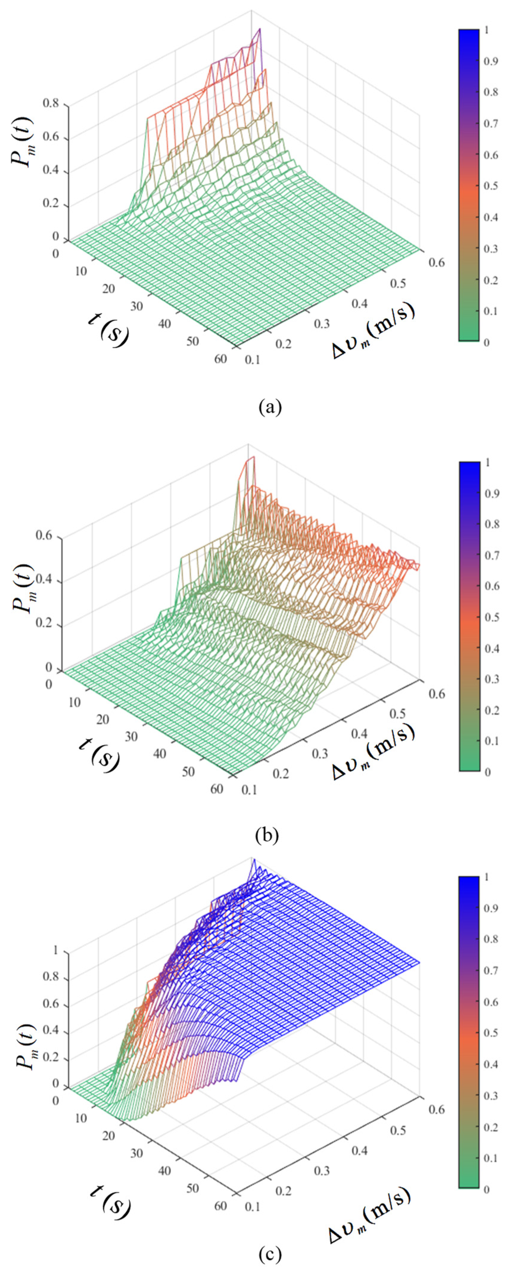
As seen in Figure 5a, $P_m(t)$ increases with $\Delta {\upsilon }_m$ and decreases with t for $\alpha =0$, $\Delta {\upsilon }_m>0.2 \mathrm{m}/\mathrm{s}$, and $t\le 25 \mathrm{s}$. $P_m(t)$ peaks at 0.72 with $\Delta {\upsilon }_m=0.6 \mathrm{m}/\mathrm{s}$ and t = 0 s. This is because the vehicle is more maneuverable, and if the impact of the aircraft is not taken into account, the vehicle will keep accelerating, bringing it closer to the intersection and extending the distance between itself and the aircraft. The average decline rate of $P_m(t)$ at $\Delta {\upsilon }_m\ge 0.4 \mathrm{m}/\mathrm{s}$ and $t\in [0 \mathrm{s},10 \mathrm{s}]$ is 0.052. When t > 25 s and $P_m(t)\approx 0$, it signifies that after 25 s, the vehicle and aircraft have developed a specific distance between them, and there is no chance that the aircraft will arrive at the junction first and pass safely.

Figure 5b illustrates that when $\alpha =0.5$, if $\Delta {\upsilon }_m\le 0.2 \mathrm{m}/\mathrm{s}$, $P_m(t)\approx 0$. $P_m(t)$ has a positive correlation with both $\Delta {\upsilon }_m$ and t if $\Delta {\upsilon }_m>0.2 \mathrm{m}/\mathrm{s}$. Due to the reduced vehicle sensitivity, the safety deceleration range is small, the separation between the aircraft and the vehicle grows slowly, and the increase of $P_m(t)$ with t is relatively small. Further analysis shows that $P_m(t)$’s growth rate is related to both $\Delta {\upsilon }_m$ and t. When $\Delta {\upsilon }_m\in (0.2 \mathrm{m}/\mathrm{s},0.5 \mathrm{m}/\mathrm{s})$, $P_m(t)$ grows on average at a rate of around 0.0018; when $\Delta {\upsilon }_m\ge 0.5 \mathrm{m}/\mathrm{s}$, $P_m(t)$ grows on average at a pace of 0.0043; and when $t\in [50 \mathrm{s},60 \mathrm{s}]$, $P_m(t)$ grows on average at a rate of 0.007. It is clear that when approaching the intersection, an increase or decrease in aircraft speed can cause appropriate vehicle deceleration behavior, which can improve traffic safety in a short time.

When $\alpha =1.0$, $P_m(t)$ has a positive correlation with both $\Delta {\upsilon }_m$ and t, as seen in Figure 5c. If t > 25 s, $P_m(t)$’s average growth rate per second is 0.02. It implies that the vehicle adjusts its speed with the aircraft as a reference, the separation can be established quickly, and the minimum separation is just 50 m because the aircraft is in front of the vehicle. As a result, the condition of Formula (15) can be easily satisfied. When $\Delta {\upsilon }_m<0.3 \mathrm{m}/\mathrm{s}$, the proportion of probability values exceeding 0.8 (also known as the high probability ratio) is 0.55, with a mean value of 0.69 and a standard deviation of 0.35. When $\Delta {\upsilon }_m\in [0.3 \mathrm{m}/\mathrm{s},0.5 \mathrm{m}/\mathrm{s})$, the high probability ratio is 0.91, with a mean value of 0.95 and a standard deviation of 0.12, and when $\Delta {\upsilon }_m\ge 0.5 \mathrm{m}/\mathrm{s}$, the high probability ratio is 0.98, with a mean value of 0.98 and a standard deviation of 0.06. This shows that vehicles traveling with high sensitivity can enhance the safety of aircraft crossing the intersection first, and the flexibility of aircraft to adjust their speed can reduce the fluctuation of safety level.

4.4. Safety Assessment Comparison and Discussion

When $\alpha =0$, we can see that if $\Delta {\upsilon }_m\le 0.2 \mathrm{m}/\mathrm{s}$, then $P_n(t)=P_m(t)=0$ comparing Figure 4a and Figure 5a. We can obtain $P_n(t)>P_m(t)$ when $\Delta {\upsilon }_m>0.2 \mathrm{m}/\mathrm{s}$ and $t\in [20 \mathrm{s},60 \mathrm{s}]$. The mean value of $P_n(t)$ is 0.45, which is 140 times that of $P_m(t)$, and the high probability ratio of $P_n(t)$ is 100% only when $\Delta {\upsilon }_m\ge 0.5 \mathrm{m}/\mathrm{s}$ and $t\in [50 \mathrm{s},60 \mathrm{s}]$.

When $\alpha =1.0$, the overall pattern of the safety probability data in Figure 4c and Figure 5c is contrary. If $t>20 \mathrm{s}$, then $P_n(t)<P_m(t)$ and the high probability ratio of $P_m(t)$ is 79%.

The overall trend of the data in Figure 4b and Figure 5b is essentially the same when $\alpha =0.5$. When $\Delta {\upsilon }_m<0.4 \mathrm{m}/\mathrm{s}$, $P_n(t)>P_m(t)$, and $P_n(t)<P_m(t)$ when $\Delta {\upsilon }_m\ge 0.4 \mathrm{m}/\mathrm{s}$, which proves that the difference between $P_n(t)$ and $P_m(t)$ is positively linked with both $\Delta {\upsilon }_m$ and t. The mean value of $P_m(t)$ is 0.524, which is 2.38 times that of $P_n(t)$ when $\Delta {\upsilon }_m=0.6 \mathrm{m}/\mathrm{s}$ and $t>40 \mathrm{s}$.

Based on the above analysis, the following conclusions are obtained.

(1)

When $\alpha =0$, it is safer for the vehicle to cross the intersection first, but whether it can do so without colliding with an aircraft depends on how the aircraft regulates its speed. If the aircraft’s speed change is minimal, there is a 100% chance of a collision at the crossing. In actual operation, when vehicles completely ignore aircraft due to poor visibility caused by fog or when the driver cannot observe aircraft due to the occlusion of terminals and obstacles, the controller should notify the pilot promptly to observe and slow down in time and remind pilots to adjust speed to avoid vehicles before reaching critical road intersection.

(2)

When $\alpha =0.5$, the safety of an aircraft passing an intersection is slightly higher than it is for a vehicle, indicating that when the vehicle safety sensitivity is low, the interval adjustment is relatively slow and both the vehicle and the aircraft have a chance to pass the intersection safely. However, the approach to the intersection will stimulate the deceleration behavior of the vehicle, thus forming the priority passage of aircraft under vehicle avoidance.

(3)

When $\alpha =1.0$, the safety probability value of the aircraft passing the intersection first is the highest. Vehicles respond sensitively to the position of the aircraft, slowing down in time and gradually increasing the separation of the two to ensure safety, thus forming the process of vehicles maintaining a low speed and following the aircraft through the intersection in turn.

(4)

The relationship between $\Delta {\upsilon }_m$ and the safety probability of cross-motion of a mixed vehicle and an aircraft is essentially positive, suggesting that the pilot’s capacity to adjust the speed and the proper amplification of the speed range can be beneficial to the separation establishment and operational safety. Additionally, the operational risk can be raised by the existing driving strategy of steady-speed taxiing, which is primarily advocated by different airline divisions to maintain taxiing stability.

5. Mixed Traffic Flow Capacity and Efficiency Analysis

The operational effectiveness of mixed traffic flow is largely determined by the safe crossing time of a vehicle and an aircraft. Let’s say that the vehicle and the aircraft depart from point O at distances $G_n(t_0)$ and $G_m(t_0)$, respectively. we define passage time as the period between when the aircraft and vehicle begin to taxi and when they are safe to cross the intersection. A safety rule is mandatory during simulation: if the intersection is occupied, the vehicle or aircraft must hold outside of it and wait until it is vacant to compute how long it will take for vehicles and aircraft to pass through the intersection without colliding.

Modify the simulation procedure in the previous section to calculate the passing time of vehicles and aircraft. $T_n$ represents the time for a vehicle leaving the intersection, $T^{\prime }$ represents the time for vehicles and aircraft to pass the intersection in sequence without conflict. Set the following parameters with common transport models and special vehicles: $L_m$ = 40 m, $L_n$ = 5 m. The following parameters are initially set for the simulation, $v_m(t_0)=v_n(t_0)$ = 5 m/s. Set the following parameters according to the control rules [34,35,36]. $S_{n,m}^{\min }$ = 200 m, $S_{m,n}^{\min }$ = 50 m, $v_m^{\max }$ = 13.8 m/s, $v_n^{\max }$ = 12.5 m/s, $\Delta {\upsilon }_n$ = 1.5 m/s. Assuming that the two are on separate taxiways and are separated by a distance of 700 m from point O, $G_m(t_0)=G_n(t_0)$ = 700 m.

In the simulation, the following three variables are predetermined: ① vehicle safety sensitivity $\alpha$, so that $\alpha \in [0,1]$ increases by 0.04 after each simulation. ② aircraft speed variance $\Delta {\upsilon }_m$, so that $\Delta {\upsilon }_m\in [0.1 \mathrm{m}/\mathrm{s},0.6 \mathrm{m}/\mathrm{s}]$ rises by 0.02 m/s after each simulation. The aforementioned simulation method will be performed 500 times to obtain the average after each simulation has produced 26 × 26 results and the random influence of a uniform distribution of speed has been removed.

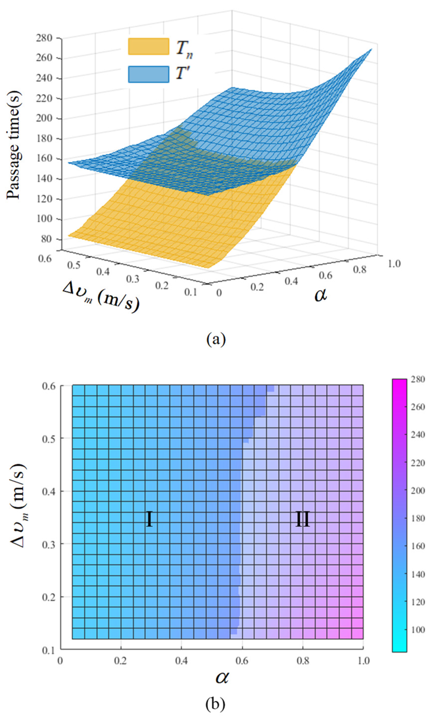
The two sets of data for $T_n$ and $T^{\prime }$ have similar trends, as seen in Figure 6a. $T_n$ and $T^{\prime }$ are both proportional to $\alpha$, showing that increased vehicle sensitivity to safety will result in deceleration when it is bigger and that frequent deceleration will result in longer passage times and worse efficiency. When $\Delta {\upsilon }_m$ is greater, the frequency of vehicle deceleration can be reduced by the driver and pilot’s flexible speed adjustment to achieve separation autonomous establishment, therefore, $T_n$ and $T^{\prime }$ and $\Delta {\upsilon }_m$ are inversely proportional. The greatest value of $T^{\prime }$ is 280 s for $\alpha$ = 1.0 and $\Delta {\upsilon }_m$ = 0.1 m/s, which is 1.8 times the minimum value. The $T_n$ surface is lower than the $T^{\prime }$ surface when $\alpha$ is smaller, indicating that the vehicle is now passing through the intersection before the aircraft. The two surfaces of $T_n$ and $T^{\prime }$ overlap when $\alpha$ is larger, suggesting that the vehicle reaches the intersection after the aircraft at this moment.

The relationship between the order of passage and the parameters $\alpha$ and $\Delta {\upsilon }_m$ may be found in Figure 6b, which is the top view of Figure 6a. Analysis reveals that when $\alpha$ and $\Delta {\upsilon }_m$ have different values, the passage process may be divided into two phases: phase I, when the vehicle crosses the intersection before the aircraft and $T_n<T^{\prime }$, and phase II when the vehicle crosses the intersection after the aircraft and $T_n=T^{\prime }$. Where the mean value of $T^{\prime }$ in region I is 157 s and the standard deviation is 3, indicating that both the passing time and its variation are minor in this region, in contrast to the mean value and standard deviation of region II, which are 1.25 times and 8.6 times of the former. It shows that the operation in a region I is more effective and stable. When $\alpha \in [0.4,0.6]$, the separation between $T^{\prime }$ and $T_n$ is close to the minimum separation standard and the difference value between the two is smaller. This means that after a vehicle or aircraft leaves an intersection, other vehicles or aircraft immediately enter the intersection, the timing of vehicles and aircraft occupying the intersection successively is closely connected, and the passage efficiency is higher. According to Figure 4 and Figure 5, at this time, whether the vehicle or aircraft first through the intersection has a high probability of safety. It implies that vehicles and aircraft can alternate and pass more effectively when $\alpha \in [0.4,0.6]$.

Set in the taxiway upstream of the intersection, 700 m from the point O, constantly having vehicles and aircraft moving forward at a speed of 5 m per second, simulating the flow of vehicles and aircraft through the intersection for 6000 s while counting the number of vehicles and aircraft N and M. Figure 7 shows the trend of change when $\alpha =\{0,0.5,1.0\}$, λ with time t. Define λ as the fraction of vehicle and aircraft passing, the value of the N and M ratio.

As observed in Figure 7, when $\alpha =1.0$, λ steadily declines with time and has an inverse relationship to $\Delta {\upsilon }_m$. With a mean value of 0.257 and a standard deviation of 0.063 at $\Delta {\upsilon }_m>0.2$ m/s and t > 3000 s, the value of λ is essentially consistent, indicating that the ratio of a vehicle to aircraft passage is roughly 1:4. The vehicle-to-aircraft ratio is currently 1:1 when $\alpha = 0.5$, λ changes insignificantly with t and $\Delta {\upsilon }_m$, and λ has a mean value of around 0.99 and a standard deviation of 0.025. λ is proportional to both t and $\Delta {\upsilon }_m$ for $\alpha = 0$. The ratio of a vehicle to aircraft passage is almost 3:1 for $\Delta {\upsilon }_m$ > 0.3 m/s and t > 3500 s when the value of λ is essentially stable with a standard deviation of 0.13 and a mean value of about 2.67.

As can be observed, the proportion of aircraft passage is higher when $\alpha$ is larger, the proportion of vehicle passage is higher when $\alpha$ is less, and the ratio of the two is better balanced when $\alpha = 0.5$. Figure 6 and Figure 7 can be compared to show that the vehicle and aircraft passage is more effective and balanced when $\alpha \in [0.4,0.6]$. By establishing vehicle speed regulation rules in the upstream taxiway of the intersection, which naturally creates the traffic flow conforming to a certain mixing ratio, the special vehicle safety sensitivity $\alpha$ has a regulating effect on the traffic flow mixing ratio, which can be adjusted according to the operation of different taxiways and the actual demand.

6. Conclusions

In this study, we create the converging operation model of aircraft and vehicles, meet the control rules and motion characteristics, and abstract the converging motion process under the mixed operation scenario of aircraft and vehicles. The following conclusions are reached through simulation verification based on a dynamic evaluation of the safety and passage efficiency under various passage strategies based on the real-time position and speed of aircraft and vehicles.

• Vehicle safety sensitivity is inversely proportional to the probability of vehicle priority passing through the intersection without conflict and is directly proportional to the probability of aircraft priority passing through. The safety sensitivity of vehicles is inversely proportional to the passing efficiency and is directly proportional to the passing ratio of aircraft.
• Vehicle safety sensitivity and deceleration rules determine the passage order of vehicles and aircraft in a short local scope and affect the passage proportion of vehicles and aircraft in the long-term multi-area range.
• The increase and decrease in aircraft taxiing speed are proportional to safety and efficiency, which indicates that even if the control rules stipulate that the driver should take the initiative to take measures, the pilot’s initiative of separation and speed adjustment should not be removed.
• A mixed traffic flow with higher safety and efficiency, better stability, and balanced locomotive proportion can be achieved when $\alpha \in [0.4,0.6]$.
• To further improve the safety of airport operations, it is possible to consider reducing the factors that contribute to the unsafe conditions of vehicle and aircraft operations during the airport planning stage. For example, expanding the airport area to reduce congestion during operations [40]. Another option is to optimize the airport runway and taxiway structures using the minimum distance model [41] after adjusting the appropriate parameters.

References

- Department of Development Planning, Civil Aviation Administration of China. 2021 National Civil Transport Airport Production Statistics Bulletin. 2022. Available online: http://www.caac.gov.cn/XXGK/XXGK/TJSJ/202203/P020220328389410591630.pdf (accessed on 10 April 2022).
- Jiang, L. Study on Apron Operation Safety of Special Vehicle. Civ. Aviat. Manag. 2014, 8, 73–74. [Google Scholar]
- Guo, B.; Wang, Z.J.; Pan, Y.J. The control of the aircraft ground collision or scratch risk. Civ. Aviat. Manag. 2017, 2, 105–112. [Google Scholar]
- Braaksma, J.P.; Shortreed, J.H. Improving Airport Gate Usage with Critical Path. Transp. Eng. J. ASCE 1971, 97, 187–203. [Google Scholar] [CrossRef]
- Cheung, A.; Ip, W.H.; Lu, D.W.; Lai, C.L. An aircraft service scheduling model using genetic algorithms. J. Manuf. Technol. Manag. 2005, 16, 109–119. [Google Scholar] [CrossRef]
- Mao, X.Y.; Mors, T.A.; Ac, M.; Roos, N. Agent-based scheduling for aircraft deicing. In Proceedings of the 18th Belgium-Netherlands Conference on Artificial Intelligence, Namur, Belgium, 5–6 October 2006; Benelux Association for Artificial Intelligence(Namur, Belgium), 2006; pp. 229–236. [Google Scholar]
- Heng, H.J.; Yan, X.D. Implementing airport special vehicles scheduling algorithm with multi-objective optimisation. Comput. Appl. Softw. 2016, 33, 238–242. [Google Scholar]
- Padrón, S.; Guimarans, D.; Ramos, J.J.; Fitouri-Trabelsi, S. A bi-objective approach for scheduling ground-handling vehicles in airports. Comput. Oper. Res. 2016, 71, 34–53. [Google Scholar] [CrossRef] [Green Version]
- Zhang, J.H.; Meng, Q.S. Scheduling optimization of airport special vehicle based on improved FCM and krill herd algorithm. Mach. Tool Hydraul. 2018, 46, 112–117. [Google Scholar]
- Wang, Z.R.; Li, Y.; Hei, X.H.; Meng, H.N. Research on airport refueling vehicle scheduling problem based on greedy algorithm. In Proceedings of the International Conference on Intelligent Computing 2018: Intelligent Computing Theories and Application, Wuhan, China, 15–18 August 2018; pp. 717–728. [Google Scholar]
- Zaninotto, S.; Gauci, J.; Farrugia, G.; Debattista, J. Design of a Human-in-the-Loop Aircraft Taxi Optimisation System Using Autonomous Tow Trucks. In Proceedings of the AIAA Aviation 2019 Forum, Dallas, TX, USA, 17–21 June 2019; p. 2931. [Google Scholar]
- Liu, Y.; Zhang, J.; Ding, C.; Bi, J. Modeling and heuristic algorithm of ground ferry vehicle scheduling in large airports. In Proceedings of the 19th COTA International Conference of Transportation, Nanjing, China, 6–8 July 2019; pp. 159–170. [Google Scholar]
- Zhao, Z.; Hu, L.; Qian, Y.Y.; Jin, H.; Jia, A.P. Research on Optimal Allocation Method of Aircraft Towing Rules Based on Multi-agent. J. Syst. Simul. 2022, 34, 113–125. [Google Scholar]
- Sun, D.G.; Sun, J.; Wang, M.; Kang, Q. Application of the improved Bow-tie risk analysis technology in civil airport safety. J. Saf. Sci. Technol. 2010, 6, 85–89. [Google Scholar]
- Wilke, S.; Majumdar, R.A.; Ochieng, W.Y. Airport surface operations: A holistic framework for operations modeling and risk management. Saf. Sci. 2014, 63, 18–33. [Google Scholar] [CrossRef]
- Fei, C.G.; Pan, W.P. Research on safety risk evaluation for electric special vehicle running on airport apron. Mod. Electron. Tech. 2017, 40, 34–38. [Google Scholar]
- Wang, Y.G.; Gao, Y.H. On the safety risk analysis and countermeasures of apron in large and medium sized airports. J. Saf. Environ. 2018, 18, 1716–1722. [Google Scholar]
- Zhao, X.; Malasse, O.; Buchheit, G. Verification of safety integrity level of high demand system based on Stochastic Petri Nets and Monte Carlo Simulation. Reliab. Eng. Syst. Saf. 2019, 184, 258–265. [Google Scholar] [CrossRef]
- Wang, Y.G.; Zuo, X.Y.; Xing, D.J. Risk evaluation on prevention and control of aircraft damage events owing to airport reason. J. Saf. Sci. Technol. 2020, 16, 165–171. [Google Scholar]
- Tong, X.Z. Hangzhou Airport Apron sector operation innovation mode. China High New Technol. 2020, 13, 85–86. [Google Scholar]
- Hu, X.; Lodewijks, G. Detecting fatigue in car drivers and aircraft pilots by using non-invasive measures: The value of differentiation of sleepiness and mental fatigue. J. Saf. Res. 2020, 72, 173–187. [Google Scholar] [CrossRef]
- Liu, B.F.; Tang, X.P.; Zhang, F. Risk assessment study for driverless special vehicles in airport flight area. Sci. Technol. Rev. 2021, 39, 83–91. [Google Scholar]
- Wang, X.L.; Yin, H. Identification of key conflict points in airport airfield area based on betweenness and degree entropy. J. Saf. Sci. Technol. 2022, 18, 236–242. [Google Scholar]
- Song, I.; Cho, I.; Tessitore, T.; Gurcsik, T.; Ceylan, H. Data-driven prediction of runway incursions with uncertainty quantification. J. Comput. Civ. Eng. 2018, 32, 04018004. [Google Scholar] [CrossRef]
- Zeng, H.; Zhang, H.M.; Ren, B.; Cui, L.; Wu, J. Aviation safety prediction method research based on improved LSTM model. Syst. Eng. Electron. 2022, 44, 569–576. [Google Scholar]
- Wang, X.L.; Yin, H.; He, M. Potential Conflicts Prediction of Mobile in the Airport Airfield Area Based on LSTM. J. Beijing Univ. Aeronaut. Astronaut. 2022. Available online: https://www.doc88.com/p-98839603750911.html (accessed on 28 November 2022).
- Cai, C.; Wu, K.; Yan, Y. Rapid detection and social media supervision of runway incursion based on deep learning. Int. J. Innov. Comput. Appl. 2018, 9, 98–106. [Google Scholar] [CrossRef]
- Lyu, Z.L.; Chen, L.Y. SA-FRCNN: An Improved Object Detection Method for Airport Apron Scenes. Trans. Nanjing Univ. Aeronaut. Astronaut. 2021, 38, 571–586. [Google Scholar]
- Zhu, X.P.; Zhang, T.X.; Li, J.J.; Xu, H. Wingtip Detection-Based Aircraft Gate Taxi-in Conflict Determination. J. Saf. Environ. 2022. Available online: http://www.cnki.com.cn/Article/CJFDTotal-AQHJ20221116005.htm (accessed on 10 December 2022).
- Yang, K.; Kang, R. Research on Taking off and Landing Separation of Aircrafts in Airport Category II Operation. Adv. Eng. Sci. 2019, 51, 217–225. [Google Scholar]
- Kang, R.; Yang, K. Risk assessment model of aircraft opposite taxiing conflict. China Saf. Sci. J. 2021, 31, 39–45. [Google Scholar]
- Kang, R.; Chen, J.; Yang, K. Probabilistic Model for the Crossover Convergence of Taxiing Aircraft. J. Ordnance Equip. Eng. 2019, 40, 115–118+150. [Google Scholar]
- Yang, K.; Yang, H.Y.; Zhang, J.W.; Kang, R. Effects on Taxiing Conflicts at Intersections by Pilots’ Sensitive Speed Adjustment. Aerospace 2022, 9, 288. [Google Scholar] [CrossRef]
- Order of the Ministry of Transport, PRC No.30. Civil Aviation Air Traffic Management Rules. 2017. Available online: http://xxgk.mot.gov.cn/jigou/fgs/201712/P020180116563208004963.pdf (accessed on 29 September 2017).
- Luo, J. Aerodrome Control; Civil Aviation Press: Beijing, China, 2013. [Google Scholar]
- Aircraft Pilot Guide-Ground Operations:AC-91-FS-2014-23, Department of Flight Standards, Civil Aviation Administration of China, Beijing. 2014. Available online: http://www.caac.gov.cn/XXGK/XXGK/GFXWJ/201811/P020181127316789533888.pdf (accessed on 11 October 2014).
- Zhao, L.; Liu, H.X. Study on Relationship Between Driving Behavior Characteristics and Personality Traits. J. Saf. Sci. Technol. 2016, 12, 171–178. [Google Scholar]
- Wei, T.Z.; Lin, M.; Li, C.X.; Zhu, Z.S.; Liu, H.X.; Zhu, D. Study of Driver’s Hazard Perception and Discriminant Model based on Covert Hazard. J. Saf. Sci. Technol. 2021, 17, 175–181. [Google Scholar]
- Kang, R.; Yang, K. Assessment on Cross Conflict of Vehicle and Aircraft Considering Driving Modes. J. Saf. Sci. Technol. 2023, 19, 218–223. [Google Scholar]
- Kazda, A.; Sedláčková, A.N.; Bračić, M. Expropriation and airport development. Civ. Environ. Eng. 2020, 16, 282–288. [Google Scholar] [CrossRef]
- Havel, K.; Balint, V.; Novak, A. A number of conflicts at route intersections—Rectangular model. Commun. Sci. Lett. Univ. Žilina 2017, 19, 145–147. [Google Scholar] [CrossRef]
Figure 1.
Simulation of Vehicle and Aircraft Convergence in the Intersection. (a) Before cross convergence; (b) After cross convergence.
Figure 2.
Scenarios of Vehicle-Aircraft Cross Convergence. (a) A vehicle crosses the intersection first; (b) Aircraft crosses the intersection first.
Figure 3.
Structure diagram of vehicle and aircraft convergence motion simulation.
Figure 4.
The trend of safety probability with safety sensitivity and time when a vehicle is first. (a) ; (b) ; (c) .
Figure 5.
The trend of safety probability with safety sensitivity and time when aircraft is first. (a) ; (b) ; (c) .
Figure 6.
Variation trend of travel time. (a) Three-dimensional figures; (b) two-dimensional figures.
Figure 7.
Fraction of vehicles and aircraft passing through the intersection under different safety sensitivities.
Disclaimer/Publisher’s Note: The statements, opinions and data contained in all publications are solely those of the individual author(s) and contributor(s) and not of MDPI and/or the editor(s). MDPI and/or the editor(s) disclaim responsibility for any injury to people or property resulting from any ideas, methods, instructions or products referred to in the content. |
© 2023 by the authors. Licensee MDPI, Basel, Switzerland. This article is an open access article distributed under the terms and conditions of the Creative Commons Attribution (CC BY) license (https://creativecommons.org/licenses/by/4.0/).
Share and Cite
MDPI and ACS Style
Yang, K.; Yang, H.; Zhang, J.; Kang, R. Safety and Efficiency Evaluation Model for Converging Operation of Aircraft and Vehicles. Aerospace 2023, 10, 343. https://doi.org/10.3390/aerospace10040343
AMA Style
Yang K, Yang H, Zhang J, Kang R. Safety and Efficiency Evaluation Model for Converging Operation of Aircraft and Vehicles. Aerospace. 2023; 10(4):343. https://doi.org/10.3390/aerospace10040343
Chicago/Turabian StyleYang, Kai, Hongyu Yang, Jianwei Zhang, and Rui Kang. 2023. "Safety and Efficiency Evaluation Model for Converging Operation of Aircraft and Vehicles" Aerospace 10, no. 4: 343. https://doi.org/10.3390/aerospace10040343
Note that from the first issue of 2016, this journal uses article numbers instead of page numbers. See further details here.