
Study of Delay Prediction in the US Airport Network

Department of Management, Universitat Politècnica de Catalunya, 08222 Terrassa, Spain
*
Author to whom correspondence should be addressed.
Aerospace 2023, 10(4), 342; https://doi.org/10.3390/aerospace10040342
Submission received: 30 January 2023
/
Revised: 14 March 2023
/
Accepted: 29 March 2023
/
Published: 1 April 2023
(This article belongs to the Special Issue Advances in Air Traffic and Airspace Control and Management)
Abstract
:In modern business, Artificial Intelligence (AI) and Machine Learning (ML) have affected strategy and decision-making positively in the form of predictive modeling. This study aims to use ML and AI to predict arrival flight delays in the United States airport network. Flight delays carry severe social, environmental, and economic impacts. Deploying ML models during the process of operational decision-making can help to reduce the impact of these delays. A literature review and critical appraisal were carried out on previous studies and research relating to flight delay prediction. In the literature review, the datasets used, selected features, selected algorithms, and evaluation tools used in previous studies were analyzed and influenced the decisions made in the methodology for this study. Data for this study comes from two public sets of domestic flight and weather data from 2017. Data are processed and split into training, validation, and testing data. Subsequently, these ML models are evaluated and compared based on performance metrics obtained using the testing data. The predictive model with the best performance (in choosing between logistic regression, random forest, the gradient boosting machine, and feed-forward neural networks) is the gradient boosting machine.
1. Introduction
Air transport is an important element of the economic system, as it has been an important means of long-distance traveling for decades. Consequently, dysfunctionality within air transport, such as flight delays, can cause large economic losses. A study from 2013 [1] showed that a decrease of only 10% in flight delays could result in a $17.6 billion increase in the US net worth, and a decrease of 30% could result in a staggering $38.5 billion increase in US net worth. Flight delays also have a severe impact on the environment. A study from 2018 [2] showed that in 2017, the extra emissions due to flight delays were estimated at 5529 tonnes, while excess fuel usage was estimated at 1,752,937 L. The deployment of machine learning models predicting flight delays could lead to a significant improvement in air transport, along with economic benefits and a smaller environmental footprint. Several approaches have been made to better understand the mechanisms of flight delays. The availability of flight data allows, for instance, examining how delays propagate along different time scales [3,4,5,6]. Another approach is to develop machine learning models that allow predicting arrival or departure delays [7,8]. Most of the proposed models are classification jobs, where the objective is to determine whether a flight will have a delay larger than a threshold value. Following the Bureau of Transport Statistics, it is commonplace to consider a flight delayed if its delay time is longer than or equal to 15 min. Other approaches, such as numerical prediction models [9] or prediction of the delay distribution [10] are also present in the literature.
The research on models predicting flight delays has increased significantly in recent years, and significant progress has been made regarding feature selection and the use of machine learning algorithms. However, most of these studies have used small sample datasets along with small-scale models to predict delays. We believe that the potential for deploying machine learning models to predict arrival delays for multiple airports has not yet been fulfilled.
The aim of this study is to test different models that predict arrival flight delays in the United States airport network. We use flight data from the Bureau of Transportation Statistics and weather data from the National Oceanic and Atmospheric Administration. This allows us to define features related to air traffic and weather to predict delays. We train several machine learning techniques suited to tabular data, such as logistic regression, random forest, the gradient boosting machine, and the feed-forward neural network model. The performance of the resulting models is then evaluated on a test set with a set of classification metrics. The four models are compared and the best-performing model is proposed as a solution for arrival delay prediction in the United States airport network.
We contribute to the literature on flight delay prediction by testing different machine learning models with a rich dataset of multiple origin and destination airports, including features related to air traffic data and weather. We also contribute by introducing mechanisms to tackle imbalanced data in the prediction workflow when doing this comparison. Flight delay prediction is an imbalanced classification problem, as there are more flights that are on time than delayed, and this can distort the results of classification models. Finally, we define explicitly a predictive modeling workflow, including training and testing in different datasets, and using validation samples and cross-validation for hyperparameter tuning.
2. Literature Review
This section presents a literature review of previous studies that have dealt with arrival and departure flight delay prediction. The results of previous studies on chosen data, selected features, algorithms, and evaluation of results are presented.
2.1. Data Used
A key element for delay prediction is obtaining flight data. The most cited source of flight data is the Bureau of Transportation Statistics [11] of the United States Department of Transportation [7,8,9,12]. Another common source of flight data is the Civil Aviation Administration of China [13,14], and in one case through VariFlight [15]. A single study [16] used a Kaggle dataset on flight data. Official sources of flight data provide reliable information to train models, and making those data open access can help to enhance the effectiveness of the covered airspace regions. Other studies rely on information from a single departure airport. This is the case in [10,17], who obtained data from Guangzhou Baiyun International Airport (ZGGG), Ref. [12] obtained data from Beijing Capital (ZBAA), and [18] obtained data from Heathrow Airport (EGLL). Finally, a=ibe study [19] relies on data from the route from Beijing Capital (ZBAA) to Hangzhou XiaoShan (ZSHC). Sometimes, authors rely on a subset of available data to build their models. In citeHu2021, flights are filtered based on the ten most significant arrival airports. In yet another study [20], both the departure and arrival airports are filtered to include one of the ten most significant airports with the most flights.
Several researchers [7,20] have used weather data, obtained through the National Oceanic and Atmospheric Administration [21]. In another study [9], weather data originates from Weather Underground [22]. Both these data sources seem reliable, the National Oceanic and Atmospheric Administration being part of the US Department of Commerce, whereas Weather Underground is a commercial source in the industry. One study [9] used a private database from the Federal Aviation Administration [23] to obtain GPS trajectory data on United States domestic air traffic.
To keep sources of data consistent, the current study chooses to pick public sources of data that originate from the US government, therefore both the Bureau of Transport Statistics, as well as the National Oceanic and Atmospheric Administration will be selected as sources of flight and weather data, respectively.
2.2. Features Chosen
The examined previous studies, except [9,17,19], included date- and date-time-related features in machine learning models predicting flight delays. In some studies [12,15,18], authors use congestion in arrival or departure airports as a feature in their predictive models. As congestion is usually related to dense traffic at peak hours, it can also be related to adverse meteorological conditions. Features related to weather are frequently used to predict delays [7,9,15,24,25]. Other features used are seating capacity [18] and automatic dependent surveillance-broadcast (ADS-B) data obtained from air surveillance systems [24,25].
2.3. Used Machine Learning Techniques
Most studies tackle delay prediction as a classification problem. The aim of these models is to determine if a flight is delayed or not. Flights are considered delayed if departure or arrival delay is above a threshold, typically 15 min. A different approach is taken in [10], where the objective is predicting delay distribution using neural networks. The authors of [9] study the numerical prediction problem, which aims to predict the delay of each flight.
Regarding machine learning techniques, studies can be classified into two broad groups. In the first group, we can include studies using deep learning techniques, frequently convolutional neural networks [10,13,14,15,20,24]. The other group of studies uses other techniques, most of them based on decision trees or ensemble techniques. Among these, random forest [8,17,18] and gradient boosting [12,16] have been especially effective in the classification models of flight delays.
Flight delay prediction is a classification problem with class imbalance, as there are more on-time flights than delayed flights. The authors of [7] found that applying undersampling to the training data improves performance and that oversampling does not improve model performance for the delay prediction problem.
In this study, we will adopt the approach of the second group and we will be using techniques based on regression and in decision trees and ensembles. We will also apply undersampling to tackle class imbalance.
2.4. Evaluation Methods Used
In some studies [9,17,20], it is unclear whether a training test data split has been used, therefore it is difficult to say whether their model configuration contains any form of overfitting and if their model is properly trained. In these studies, no testing set is mentioned and only evaluation metrics based on the training data are given. Some studies [17,20] only use accuracy as an evaluation metric. It is important to use several different model evaluation metrics to have a proper insight into the performance of the model. Therefore, it is important to also use the area under the curve (AUC) of the receiver operating characteristic curve (ROC), as used in [7,18]. One paper [18] uses a more elaborate method of model evaluation including several important model evaluation metrics, such as precision, recall, and the F1 score. To have proper insight into model performance, in this study, a set of classification metrics will be evaluated to choose the best-performing model. These metrics will include, accuracy, recall, precision, F1 score, and ROC AUC. In addition to these metrics, the area under the precision-recall curve (PR AUC) will also be used, as this is an important metric to use in imbalanced datasets, as well as specificity, which gives an indication of the performance of detecting true negatives. Those metrics will be obtained from a test set, and hyperparameter tuning and model selection will be performed using cross-validation or splitting the data into train, validation, and test sets.
3. Methodology
We present, in this section, the following methodological traits of the evaluation of the competing flight delay prediction models: the description of the datasets used, the data preprocessing workflow, the hyperparameter tuning of the different models, and the model evaluation.
3.1. Datasets Used
This study uses flight data of the United States from 2017 obtained through the open database of the United States Bureau of Transport Statistics [11]. The raw dataset has 5.7 million flights and includes attributes in three different categories of attributes: date and time, scheduling time, and flight. The date and time-related attributes include the quarter, the month, the day of the month, the day of the week, the hour of the day, and the minutes of the hour. These attributes, their type, and examples are shown in Table 1.
The scheduling time-related attributes include the planned departure and arrival times, the actual departure and arrival times, the planned and actual arrival and departure at the local time, the wheels on and off time, and the wheels on and off at the local time. These attributes, their type, and examples are shown in Table 2.
Flight-related attributes include the carrier, the tail number, the flight number, the origin airport, the destination airport, the flight distance, and the seating capacity. These attributes, their type, and examples are shown in Table 3.
In addition to flight data, the weather data for both the origin and destination airport from 2017 is obtained through the open database of the United States National Oceanic and Atmospheric Administration [21]. The data consists of the daily average of the wind speed, the wind direction, the air temperature, the atmospheric pressure, the visibility, the dew point, the precipitation, the cloud cover, the wind gust, and the total snow. These attributes, their type, and examples are shown in Table 4.
3.2. Data Preprocessing
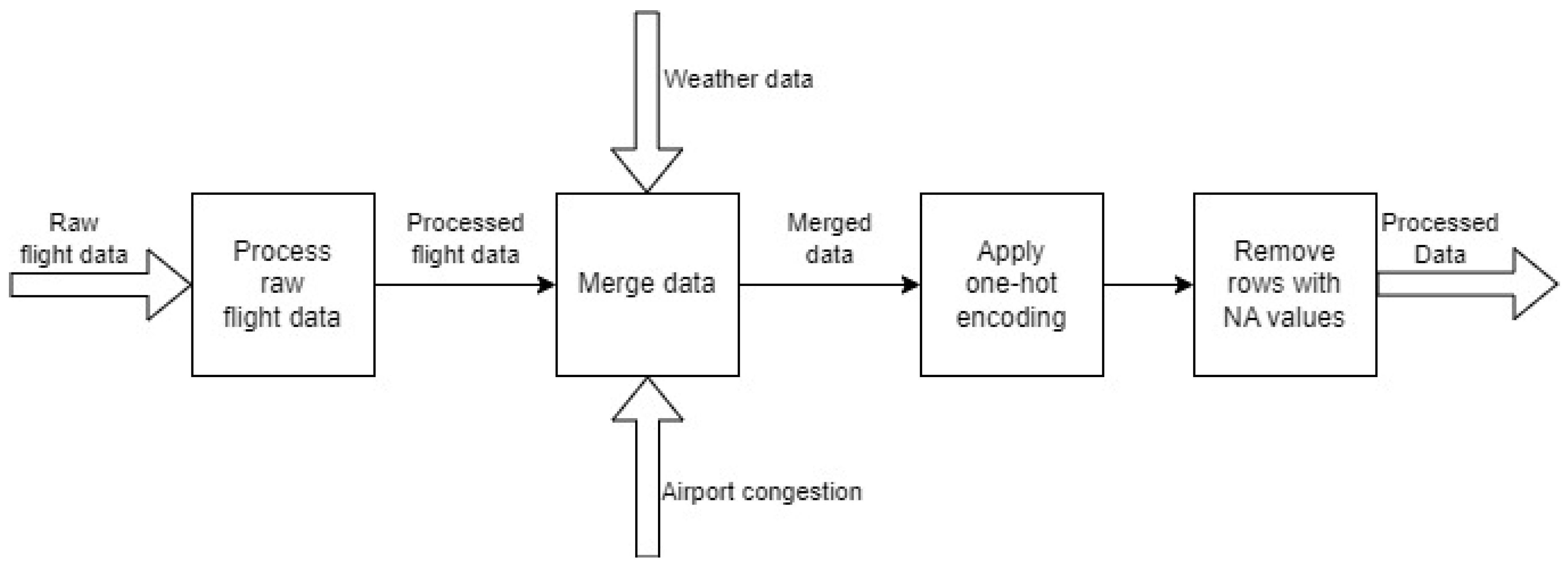
After obtaining the raw flight and weather data, the next step is to preprocess these data before splitting. A high-level overview of the data processing steps is given in Figure 1.
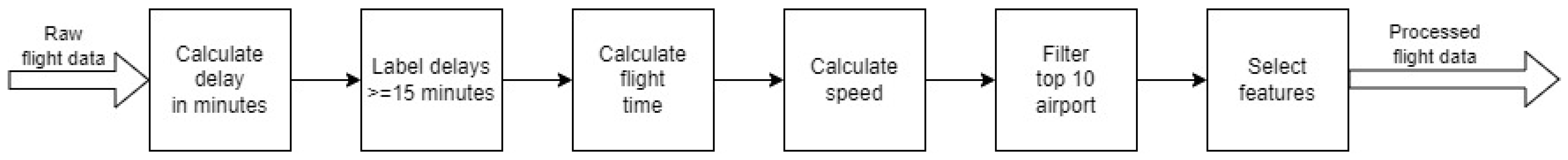
At first, the raw flight data mentioned in Table 1, Table 2 and Table 3 are processed in a data pipeline. The processed flight data are then merged with weather data and airport congestion. Airport congestion is measured as the total number of arriving and departing flights per day at a specific origin or destination airport. Next, the categorical variables in the obtained merged dataset are transformed using one-hot encoding. Lastly, any rows with any number of empty values are removed. The data processing pipeline for the flight data is shown in Figure 2.
This study explores the possibility of prediction of arrival delays, therefore, the first step in the data pipeline is to calculate this arrival delay. The arrival delay is calculated using the actual arrival time and the planned arrival time. As per the definition of the Bureau of Transport Statistics, any flight that experiences a delay equal to or greater than 15 min is considered delayed, and any flight with a delay smaller than 15 min is considered on time. Therefore, in the second step of the proposed data pipeline, the delay target variable is labeled using a threshold of 15 min applied to the calculated arrival delay as shown in Equation (1).
Once obtained the target variable, two additional features are calculated: the planned flight time and the planned flight speed. The planned flight time is calculated using the planned departure time and the planned arrival time and is shown in Equation (2). The planned flight speed is calculated by dividing the flight distance by the flight time, this is shown in Equation (3).
After engineering and adding these two features, the data are filtered by the top 10 airports with the most flights. Therefore, we only consider flights happening between these top 10 airports. A list of the top 10 airports for both the origin and destination is given in Table 5.
After processing the data as described above and as shown in Figure 1 and Figure 2, the resulting dataset consists of 36 variables. These variables consist of the target variable delay, and the 35 features used to predict this target variable. The resulting data can be categorized into the following categories: date-time and scheduling-based features, flight and airport-based features, and weather-based features for both the origin and destination airports. The date-time and scheduling-based features used to predict arrival delays are given in Table 6. The flight and airport-based features used to predict arrival delays are also given in Table 6.
The final selected weather features are shown in Table 7. These weather features are included for both the origin as well as the destination airport.
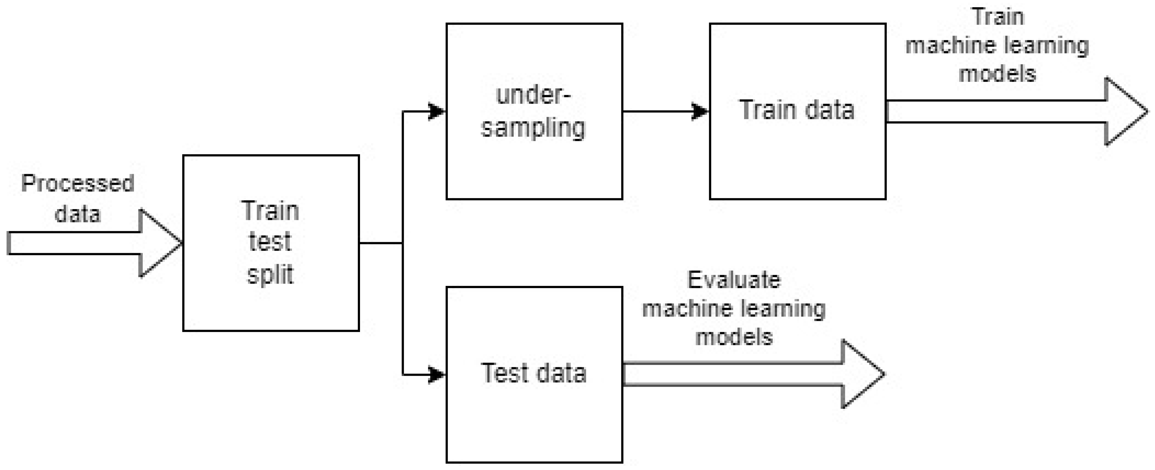
After obtaining the final data with the features summarized in Table 6 and Table 7, a train-test and train-validation-test split are performed. The flight data are highly imbalanced, with the number of delayed flights in the raw data being only 18% of the total, and the majority of 82% being on-time flights. To improve model performance, the training data are under-sampled. Two of the four models are trained using the Spark framework and two of the four models are trained using the H2O framework. For the models trained using the Spark framework, the data are split into training and testing data, with 90% of the data going into the training data and 10% of the data going into the testing data. During the data split, stratification is applied to ensure a similar ratio of delayed and non-delayed flights in the data split, and after splitting the data, the majority class in the training data is undersampled. This process is also shown in the diagram in Figure 3. By undersampling the majority class in the training dataset, the number of delayed flights is made equal to the number of non-delayed flights, respectively, by randomly removing rows. The training data are used to train the machine learning models and the testing data are used to evaluate the machine learning model performance on unseen data.
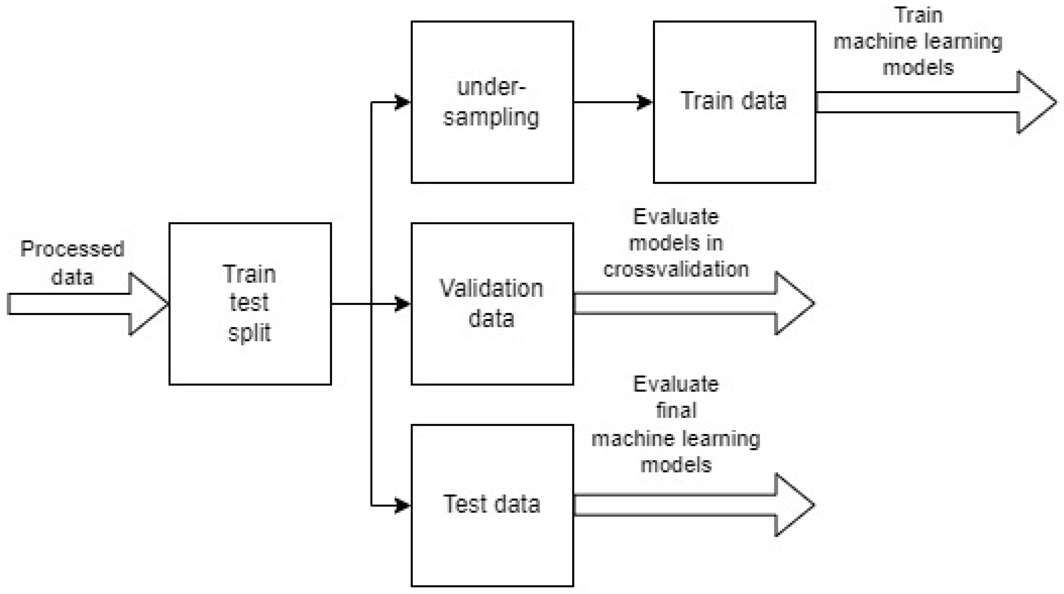
For the models trained using the H2O framework, the data are split into training, validation, and testing data, with 80% of the data going into the training data set, 10% into the validation data set, and 10% in the training data set. The training data is undersampled similar to the training-testing data split mentioned above. This process of splitting the data into training, validation, and testing data is shown in Figure 4. The training data is used to train the machine learning models, the validation data is used for performance evaluation and the testing data is used to evaluate the machine learning model performance on unseen data.
3.3. Hyperparameter Tuning
Each model will be tuned to find the optimal parameters. The parameters used in the hyperparameter tuning and their corresponding values can be seen in the overview in Table 8. In addition to the hyperparameter tuning, each model will be cross-validated four-fold.
3.4. Model Evaluation
To evaluate the classification models, we use the testing data obtained through the data split shown in Figure 3 and Figure 4. For each model, a confusion matrix will be constructed as shown in Table 9 from predictions made on the unseen data in the testing dataset.
The first model metric used is accuracy. Accuracy is defined as the fraction or percentage at which the model predicted correctly in all of the predictions [26]. The equation for accuracy is shown in Equation (4) [26]. Accuracy can be a deceiving evaluation metric in imbalanced datasets [26]. A poorly performing model can have moderate or even high accuracy, and a properly performing model can have low accuracy [26]. This is the reason to combine multiple model evaluation metrics to have a better understanding of model performance.
Misclassification rate is directly linked with accuracy, as it is the difference between 100% and the accuracy. As accuracy is defined as the percentage at which the model predicted correctly, the misclassification rate is defined as the percentage at which the model predicted incorrectly [26]. The formula for misclassification can be found in Equation (5) [26].
Recall is defined as the percentage of actual positives or actual delays that were predicted correctly. Recall says something about the model’s ability to identify actual positives correctly [26]. The formula for recall is given in Equation (6). In the flight delay study, a high recall means the model is capable of predicting actual flight delays properly, so in this study a high recall is desirable. Precision on the other hand is defined as the percentage of positive predictions that were actually correct [26]. The formula for precision is given in Equation (7) [26].
The following considered metric is the F1 score. This metric combines both precision and recall in a single metric using the harmonic mean between the two metrics [26]. As mentioned previously, accuracy can be a deceiving model evaluation metric in imbalanced datasets. This is where the F1 score comes in useful as it gives a better insight into model performance. The formula to calculate the F1 score is given in Equation (8) [26].
Specificity, which is also known as the true negative rate, says something about the models’ ability to predict true negatives [26]. In the context of flight delay prediction, this translates into the ability of the model to predict if a given flight has no delay. The formula to calculate specificity is given in Equation (9).
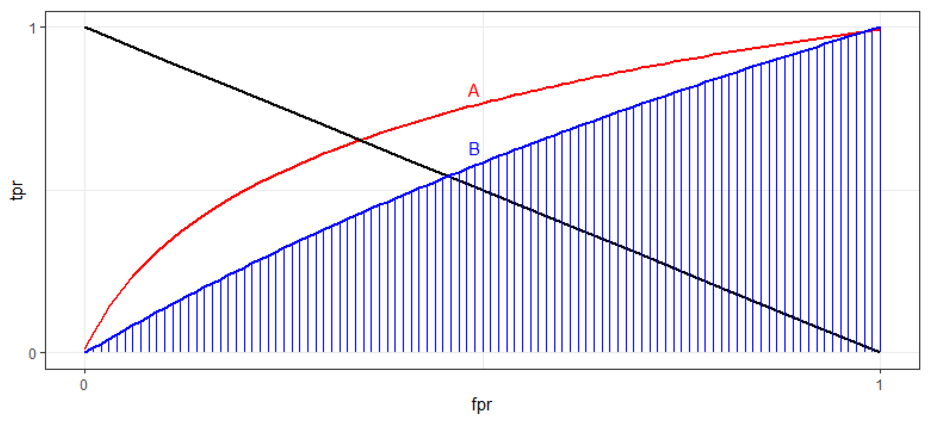
The next model metric is the area under the receiver operating characteristic (ROC) curve. Figure 5 shows an example of a ROC curve [26]. The ROC curve is an evaluation metric used in binary classification problems, it is a probability curve that plots the true positive rate against the false positive rate [26]. The area under the ROC curve (ROC AUC) gives the performance of the model when distinguishing between positive and negative classes, therefore the higher this metric the better performing the model. In Figure 5, the blue-shaded area is the AUC of ROC curve B. ROC curve A has better performance than B, thus having a higher AUC.
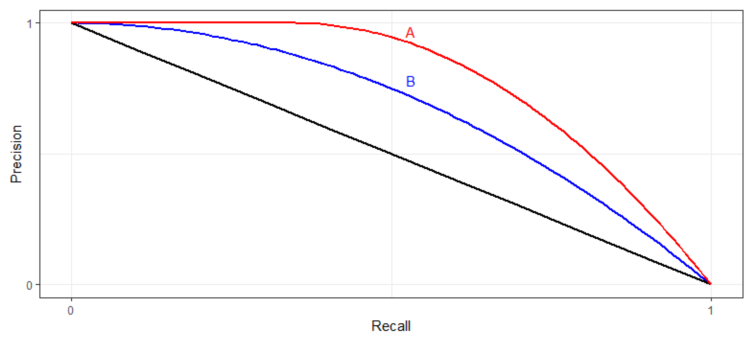
The final model metric is the area under the precision-recall curve, better known as PR AUC. Figure 6 shows an example of a PR curve [26]. The PR curve is an evaluation metric used in binary classification problems, it is a probability curve that plots the precision against the recall [26]. The area under the PR curve gives the performance of the model and an area closer to 1 indicates a better-performing model. In Figure 6, PR A has better performance than PR B, thus having a higher AUC.
4. Results
This section presents the results obtained with the process explained in the methodology section. This includes the results obtained after data processing, and the results obtained for each final, tuned, and cross-validated model. The results for the evaluation metrics obtained for each model are then compared and the best-performing model is proposed for flight arrival delay prediction.
4.1. Data Processing
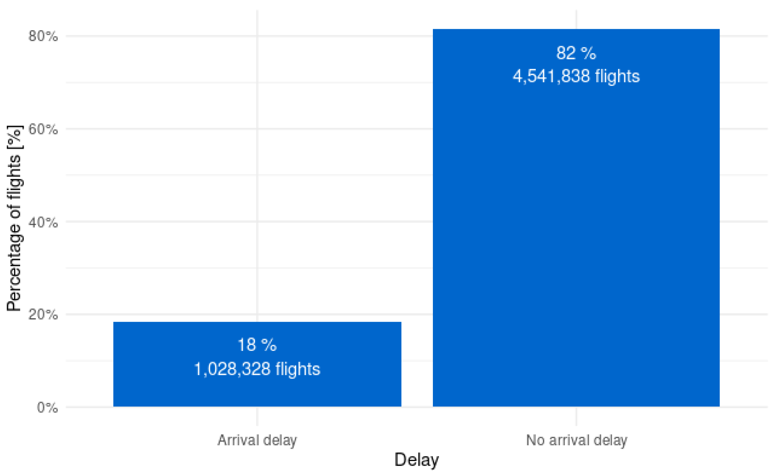
The raw flight data for 2017 includes over 5.6 million flights. When applying the definition of the Bureau of Transport Statistics to this raw data, which is that any flight with a delay greater or equal to 15 min is considered delayed, a great imbalance in the target variable is observed. Of the raw flight data, a large majority of 82% are non-delayed, and only 18% are delayed, which is also shown in Figure 7. With such an imbalance in the target variable, it is important to look at the class imbalance after preprocessing the data and applying undersampling during the majority class after the data split, as shown in Figure 3 and Figure 4.
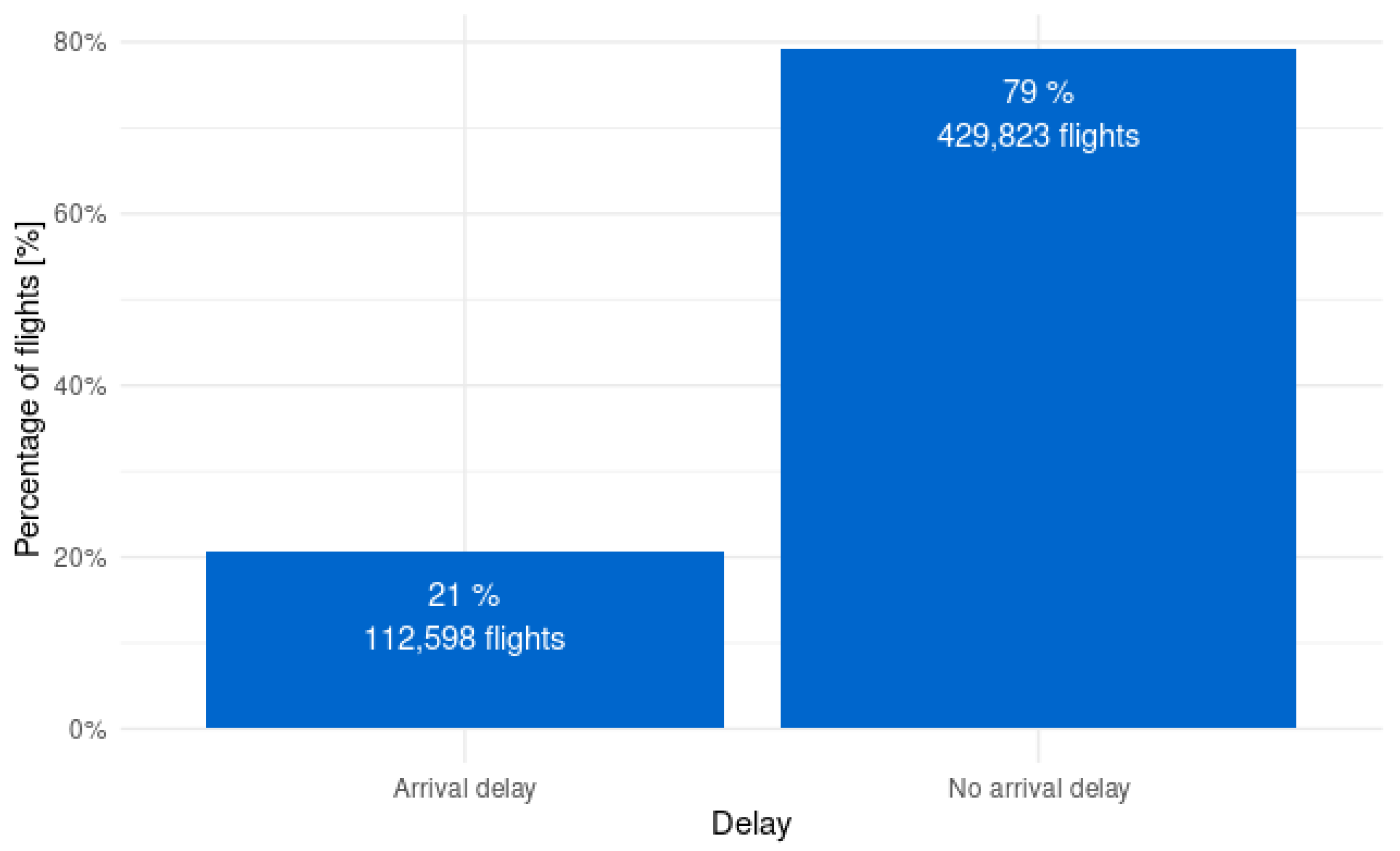
After processing the data in the pipeline and joining the weather data and the airport congestion data, there are only 542,421 rows left, which comes down to only 9.57% of the raw data. As shown previously in Figure 7, the arrival delays in the raw data were highly imbalanced. When taking a look at the imbalance in the processed data, it is clear that it is still highly imbalanced. The imbalance in the arrival flight delays of the processed data is shown in Figure 8. After processing the data, the imbalance stays in a similar ratio, with 79% of the flights being non-delayed flights and 21% of the flights being delayed flights.
4.2. Logistic Regression Results
The optimal model parameters for logistic regression are given in Table 10. The optimal parameter value for the elastic net regularization and the regularization is 0. These parameters are used to train the final logistic regression model, which is cross-validated four-fold.
To evaluate the performance of the logistic regression model, predictions are made based on testing data. The confusion matrix constructed with these results is shown in Table 11. The true positives are 7137, the false negatives are 4143, the false positives are 15,040, and the true negatives are 28,025. The evaluation metrics for the logistic regression model are given in Table 12 together with the other models. The accuracy, precision, recall, F1-score, and specificity are calculated using the equations given in the methodology. The PR AUC and ROC AUC are obtained using the calculator of Spark.
4.3. Random Forest
The optimal model parameters for random forest are given in Table 13. The optimal parameter value for the maximum depth of each tree is 10 and the number of trees is 50. These parameters are used to train the final random forest model, which is cross-validated four-fold.
To evaluate the performance of the logistic regression model predictions are made based on testing data. The confusion matrix constructed with these results is shown in Table 14. The true positives are 7428, the false negatives are 3852, the false positives are 12,626, and the true negatives are 30,439. The evaluation metrics for the random forest model are given in Table 12 together with the other models. The accuracy, precision, recall, F1-score, and specificity are calculated using the equations given in the methodology. The PR AUC and ROC AUC are obtained using the calculator of Spark.
4.4. Gradient Boosting Machine
The optimal model parameters for the gradient boosting machine are given in Table 15. The optimal parameter value for the maximum depth of each tree is 17, the row sampling rate is to be found at 0.91, the column sampling rate is found at 0.33, the column sampling rate per tree at 0.95, the minimum observations per leaf at 16, the number of bins for continuous features at 512, the number of bins for categorical features at 64, and the minimum error improvement at 0. These parameters are used to train the final gradient boosting machine model, which is cross-validated with 4-folds.
To evaluate the performance of the gradient boosting machine, model predictions are made based on testing data. The confusion matrix constructed with these results is shown in Table 16. The true positives are 9901, the false negatives are 1350, the false positives are 12,152, and the true negatives are 31,019. The evaluation metrics for the gradient boosting machine model are given in Table 12 together with the other models. The accuracy, precision, recall, F1-score, and specificity are calculated using the equations given in the methodology. The PR AUC and ROC AUC are obtained using the calculator of H2O.
4.5. Feed-Forward Neural Network
The optimal model parameters for the feed-forward neural network are given in Table 17. The optimal parameter value for the number of hidden layers is found to be 2, with 64 nodes in each layer, the input dropout ratio is found at 0.05, the learning rate is found at 0.02, and the learning rate annealing is found at . These parameters are used to train the feed-forward neural network model, which is cross-validated four-fold. The confusion matrix for the feed-forward neural network is presented in Table 18.
4.6. Model Comparison
Now that all the evaluation metrics have been obtained from the final tuned models using predictions on the test data, the next step is to compare each model and pick the best-performing model as the final solution to the flight delay prediction problem. Table 12 shows the comparison of the accuracy, F1 score, specificity, area under the ROC curve, and the area under the PR curve. When comparing the models using the evaluation metrics in Table 12, it is clear that the gradient boosting machine has the best performance among the four examined models. The gradient boosting machine wins when looking at accuracy, the F1 score, PR AUC, and ROC AUC, and beats random forest slightly in terms of specificity.
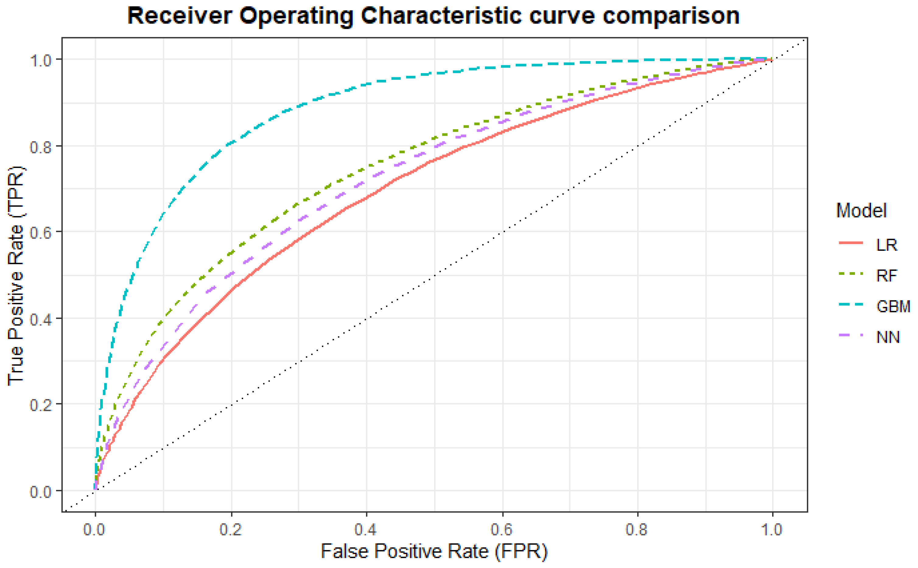
Furthermore, when looking at a comparison of the ROC curves of each model in Figure 9, the gradient boosting machine clearly has a higher ROC AUC curve. This indicates a better performance as a binary classification model. Considering ROC AUC performance, the gradient boosting machine is followed by the random forest model, the feed-forward neural network, and lastly the logistic regression model.
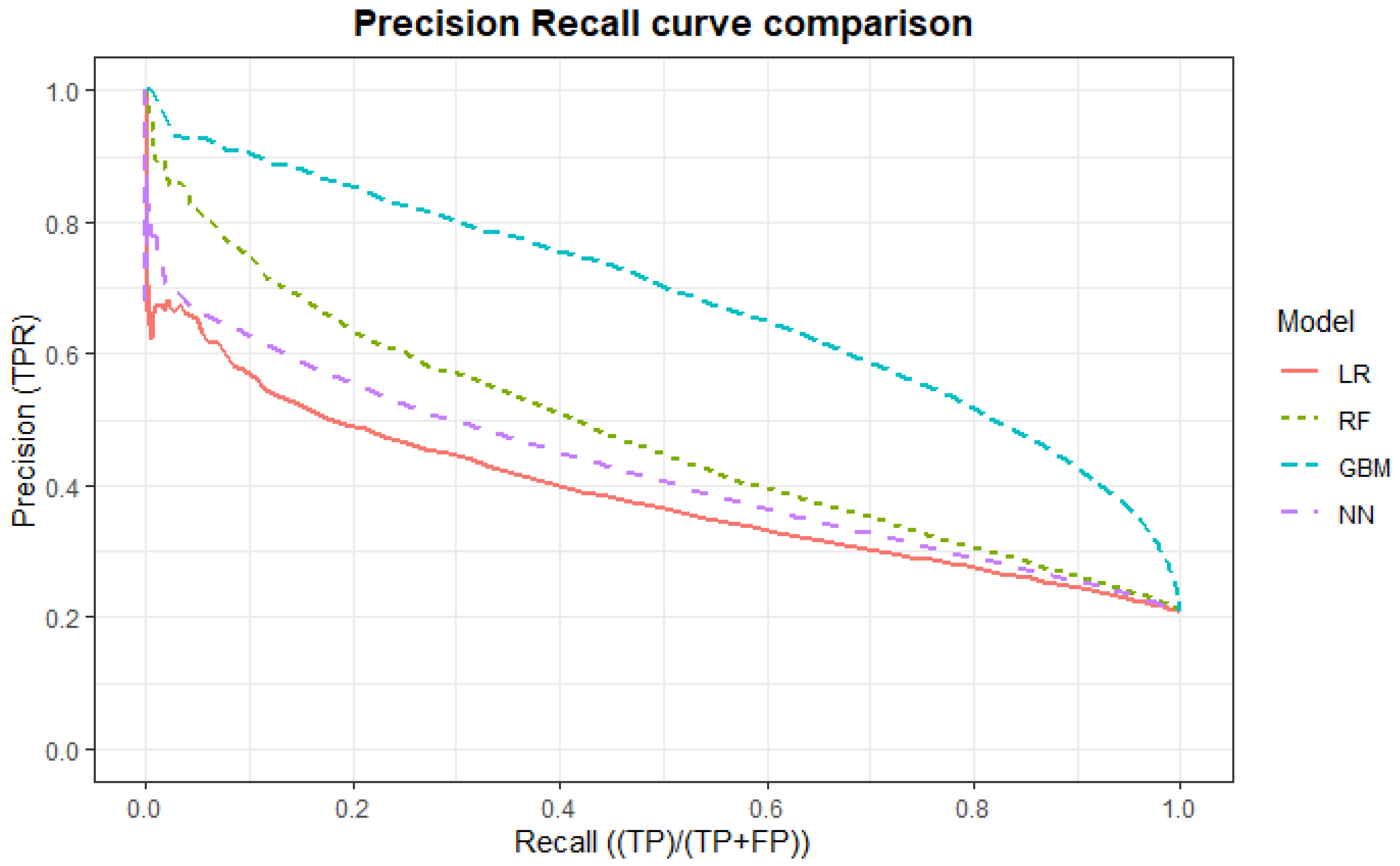
A comparison of the precision-recall curves of all models is given in Figure 10. It is clearly visible that the gradient boosting machine has the best performance among all models in terms of PR AUC. When evaluating models with PR AUC, the gradient boosting machine is again followed by the random forest model, the feed-forward neural network, and lastly the logistic regression model.
5. Discussion
The raw flight and weather data have been processed and merged together with the data on airport congestion. After processing this data and selecting the features, the data were split into training and testing data, and training, validation, and testing data, respectively. After splitting this data, hyperparameter tuning was performed for each model. Each of the four models was tuned to find the optimal performance and was cross-validated four-fold when training the final model using the optimal performance. When comparing the performance of the four models using Table 12, it is clear that the gradient boosting machine model has the best performance. The gradient boosting machine beats the other models in accuracy, precision, recall, f1-score, specificity, and the areas under the PR and ROC curves. When observing the visual model comparison in the PR curves in Figure 10 and the ROC curves in Figure 9, the gradient boosting machine clearly has the best performance among the four models. Specifically, the random forest model performs similarly to the gradient boosting machine, but in all other metrics, the gradient boosting machine has the best performance. Random forest is the second-best predictive model among the four. The logistic regression model is a very close third among the models, outperforming the feed-forward neural network in accuracy, ROC AUC, and specificity. Of the four models, the feed-forward neural network has the poorest performance. Besides having a lower accuracy, the model especially performs very poorly in specificity compared to the other models, where the other models have slightly more balanced metrics. It is interesting, however, to note that the feed-forward neural network has a much higher recall, which is shown in Table 12, compared to the other three models. The outliers in the specificity and recall indicate that this type of machine learning model is not suitable for tabular data such as the flight and weather data used in this study. Furthermore, it is important to note that all models perform poorly in precision. This poor performance in precision is also reflected in the values for the F1 score since the F1 score is directly derived from precision and recall as well. This poor performance likely comes from the highly imbalanced nature of the dataset as well as its size, with only a minority of the dataset being delayed and a large majority being on-time flights. Out of all four models, the gradient boosting machine is the best model with the best performance in all categories and, therefore, the model most suitable to perform flight delay predictions. This model seems to beat the lightGBM model, which has a similar architecture to [18], on the following evaluation metrics: F1 score with an 8% improvement, recall with a 36% improvement, and ROC AUC with a 10% improvement.
6. Conclusions
The article presents a machine learning approach to the prediction of arrival flight delays in the United States airport network. Several different models are tuned, trained, and compared using model performance which is based on predictions made on the test data. Based on this comprehensive comparison the solution for arrival delay prediction is chosen to be a gradient boosting machine model, which has higher performance in every evaluation metric applied in this study. The study allows us to draw the following conclusions:
- For arrival flight delay prediction in the United States airport network, the usage of publicly available flight and weather allows for the design of usable machine learning models.
- Between the four machine learning models chosen in this study: logistic regression, random forest, gradient boosting machine, and feed-forward neural network, the gradient boosting machine has the best performance. The gradient boosting machine beats the other three models by far across all model evaluation metrics.
The prediction of delayed flights in our model depends on features based on weather forecasts. Therefore, the available time of the prediction is the one when accurate weather forecasts are available. To that respect, our study takes a different approach compared to models performing strategic flight delay prediction, such as in [10], which only uses features available months in advance.
Author Contributions
Conceptualization, J.M.S.; methodology, K.K. and J.M.S.; software, K.K.; validation, K.K. and J.M.S.; formal analysis, K.K.; investigation, K.K.; resources, K.K.; data curation, J.M.S. and K.K.; writing—original draft preparation, K.K.; writing—review and editing, K.K. and J.M.S.; visualization, K.K. All authors have read and agreed to the published version of the manuscript.
Funding
This research received no external funding.
Data Availability Statement
Data are contained within the article.
Conflicts of Interest
The authors declare no conflict of interest.
Abbreviations
The following abbreviations are used in this manuscript:
| US | United States |
| ML | Machine Learning |
| AI | Artificial Intelligence |
| LR | Logistic Regression |
| RF | Random Forest |
| GBM | Gradient Boosting Machine |
| NN | Feed-Forward Neural Network |
References
- Peterson, E.B.; Neels, K.; Barczi, N.; Graham, T. The economic cost of airline flight delay. J. Transp. Econ. Policy 2013, 47, 107–121. [Google Scholar]
- Dissanayaka, D.; Adikariwattage, V.; Pasindu, H. Evaluation of Emissions from Delayed Departure Flights at Bandaranaike International Airport (BIA). In Proceedings of the 11th Asia Pacific Transportation and the Environment Conference (APTE 2018), Malang, Indonesia, 18–19 October 2018; Atlantis Press: Paris, France, 2019; pp. 143–146. [Google Scholar] [CrossRef] [Green Version]
- Bombelli, A.; Sallan, J.M. Analysis of the effect of extreme weather on the US domestic air network. A delay and cancellation propagation network approach. J. Transp. Geogr. 2023, 107, 103541. [Google Scholar] [CrossRef]
- Wang, Y.; Li, M.Z.; Gopalakrishnan, K.; Liu, T. Timescales of delay propagation in airport networks. Transp. Res. Part E Logist. Transp. Rev. 2022, 161, 102687. [Google Scholar] [CrossRef]
- Pastorino, L.; Zanin, M. Local and Network-Wide Time Scales of Delay Propagation in Air Transport: A Granger Causality Approach. Aerospace 2023, 10, 36. [Google Scholar] [CrossRef]
- Zanin, M. Can we neglect the multi-layer structure of functional networks? Phys. A Stat. Mech. Its Appl. 2015, 430, 184–192. [Google Scholar] [CrossRef] [Green Version]
- Choi, S.; Kim, Y.J.; Briceno, S.; Mavris, D. Prediction of weather-induced airline delays based on machine learning algorithms. In Proceedings of the 2016 IEEE/AIAA 35th Digital Avionics Systems Conference (DASC), Sacramento, CA, USA, 25–29 September 2016; pp. 1–6. [Google Scholar] [CrossRef]
- Rebollo, J.J.; Balakrishnan, H. Characterization and prediction of air traffic delays. Transp. Res. Part C Emerg. Technol. 2014, 44, 231–241. [Google Scholar] [CrossRef]
- Shao, W.; Prabowo, A.; Zhao, S.; Tan, S.; Koniusz, P.; Chan, J.; Hei, X.; Feest, B.; Salim, F.D. Flight Delay Prediction using Airport Situational Awareness Map. In Proceedings of the 27th ACM SIGSPATIAL International Conference on Advances in Geographic Information Systems, Chicago, IL, USA, 5–8 November 2019; ACM: New York, NY, USA, 2019; pp. 432–435. [Google Scholar] [CrossRef] [Green Version]
- Wang, Z.; Liao, C.; Hang, X.; Li, L.; Delahaye, D.; Hansen, M. Distribution Prediction of Strategic Flight Delays via Machine Learning Methods. Sustainability 2022, 14, 15180. [Google Scholar] [CrossRef]
- Bureau of Transport Statistics, United States Department of Transportation. Airline On-Time Statistics. Available online: https://www.transtats.bts.gov/ONTIME/ (accessed on 1 January 2023).
- Wang, X.; Wang, Z.; Wan, L.; Tian, Y. Prediction of Flight Delays at Beijing Capital International Airport Based on Ensemble Methods. Appl. Sci. 2022, 12, 10621. [Google Scholar] [CrossRef]
- Cai, K.; Li, Y.; Fang, Y.P.; Zhu, Y. A Deep Learning Approach for Flight Delay Prediction through Time-Evolving Graphs. IEEE Trans. Intell. Transp. Syst. 2022, 23, 11397–11407. [Google Scholar] [CrossRef]
- Cai, K.; Li, Y.; Zhu, Y.; Fang, Q.; Yang, Y.; Du, W. A geographical and operational deep graph convolutional approach for flight delay prediction. Chin. J. Aeronaut. 2023, 36, 357–367. [Google Scholar] [CrossRef]
- Li, Q.; Jing, R. Flight delay prediction from spatial and temporal perspective. Expert Syst. Appl. 2022, 205, 117662. [Google Scholar] [CrossRef]
- Khan, R.; Akbar, S.; Zahed, T.A. Flight Delay Prediction Based on Gradient Boosting Ensemble Techniques. In Proceedings of the 2022 16th International Conference on Open Source Systems and Technologies (ICOSST), Lahore, Pakistan, 14–15 December 2022; pp. 1–5. [Google Scholar] [CrossRef]
- Hu, P.; Zhang, J.; Li, N. Research on Flight Delay Prediction Based on Random Forest. In Proceedings of the 2021 IEEE 3rd International Conference on Civil Aviation Safety and Information Technology (ICCASIT), Changsha, China, 20–22 October 2021; pp. 506–509. [Google Scholar] [CrossRef]
- Lambelho, M.; Mitici, M.; Pickup, S.; Marsden, A. Assessing strategic flight schedules at an airport using machine learning-based flight delay and cancellation predictions. J. Air Transp. Manag. 2020, 82, 101737. [Google Scholar] [CrossRef]
- Yu, B.; Guo, Z.; Asian, S.; Wang, H.; Chen, G. Flight delay prediction for commercial air transport: A deep learning approach. Transp. Res. Part Logist. Transp. Rev. 2019, 125, 203–221. [Google Scholar] [CrossRef]
- Kim, Y.J.; Choi, S.; Briceno, S.; Mavris, D. A deep learning approach to flight delay prediction. In Proceedings of the 2016 IEEE/AIAA 35th Digital Avionics Systems Conference (DASC), Sacramento, CA, USA, 25–29 September 2016; pp. 1–6. [Google Scholar] [CrossRef]
- National Oceanic and Atmospheric Administration: Global Hourly–Integrated Surface Database (ISD). Available online: https://www.ncei.noaa.gov/products/land-based-station/integrated-surface-database (accessed on 1 January 2023).
- Weather Underground: Los Angeles International Airport. Available online: https://www.wunderground.com/history/daily/us/ca/los-angeles/KLAX/date (accessed on 1 January 2023).
- Federal Aviation Administration, United States Department of Transportation. System Wide Information Management (SWIM). Available online: https://www.faa.gov/air_traffic/technology/swim/ (accessed on 1 January 2023).
- Gui, G.; Liu, F.; Sun, J.; Yang, J.; Zhou, Z.; Zhao, D. Flight Delay Prediction Based on Aviation Big Data and Machine Learning. IEEE Trans. Veh. Technol. 2020, 69, 140–150. [Google Scholar] [CrossRef]
- Liu, F.; Sun, J.; Liu, M.; Yang, J.; Gui, G. Generalized Flight Delay Prediction Method Using Gradient Boosting Decision Tree. In Proceedings of the 2020 IEEE 91st Vehicular Technology Conference (VTC2020-Spring), Antwerp, Belgium, 25–28 May 2020; pp. 1–5. [Google Scholar] [CrossRef]
- Murphy, K.P. Machine Learning: A Probabilistic Perspective; MIT Press: Cambridge, MA, USA, 2012. [Google Scholar]
Figure 1.
High-level data processing.

Figure 2.
Flight data pipeline.

Figure 3.
Training and testing data split.

Figure 4.
Training, validation, and testing data split.

Figure 5.
ROC AUC curve example [26].
Figure 5.
ROC AUC curve example [26].

Figure 6.
PR AUC curve example [26].
Figure 6.
PR AUC curve example [26].

Figure 7.
Imbalance of arrival delays in raw flights.

Figure 8.
Imbalance of arrival delays in processed data.

Figure 9.
Comparison of the ROC curves between the different models: Logistic regression (LR), Random Forest (RF), Gradient Boosting Machine (GBM), Feed-Forward Neural Network (NN).
Figure 9.
Comparison of the ROC curves between the different models: Logistic regression (LR), Random Forest (RF), Gradient Boosting Machine (GBM), Feed-Forward Neural Network (NN).

Figure 10.
Comparison of the PR curves between the different models: Logistic regression (LR), Random Forest (RF), Gradient Boosting Machine (GBM), Feed-Forward Neural Network (NN).
Figure 10.
Comparison of the PR curves between the different models: Logistic regression (LR), Random Forest (RF), Gradient Boosting Machine (GBM), Feed-Forward Neural Network (NN).


Table 1.
Attributes related to the date and the time.
| Attribute Name | Type | Example |
|---|---|---|
| Quarter | Integer | 1, 2, 3, 4 |
| Month | Integer | 1, 2, 3, … 12 |
| Day of month | Integer | 1, 2, 3, … 31 |
| Day of week | Integer | 1, 2, 3, … 7 |
| Hour of day | Integer | 1, 2, 3, … 23 |
| Minute of the hour | Integer | 0, 1, 2, 3, … 59 |
Table 2.
Attributes related to the scheduling time.
| Attribute | Type | Example |
|---|---|---|
| Planned departure time | Date-time | 1 January 2017 01:00:00 |
| Planned departure local hour. | Integer | 0, 1, 2, 3, … 23 |
| Planned arrival time | Date-time | 2 January 2017 02:00:00 |
| Planned arrival local hour | Integer | 0, 1, 2, 3, … 23 |
| Actual departure time | Date-time | 3 January 2017 03:00:00 |
| Actual departure local hour | Integer | 0, 1, 2, 3, … 23 |
| Actual arrival time | Date-time | 4 January 2017 04:00:00 |
| Actual arrival local hour | Integer | 0, 1, 2, 3, … 23 |
| Wheels on time | Date-time | 5 January 2017 05:00:00 |
| Wheels on local hour | Integer | 0, 1, 2, 3, … 23 |
| Wheels off time | Date-time | 6 January 2017 06:00:00 |
| Wheels off local hour | Integer | 0, 1, 2, 3, … 23 |
Table 3.
Flight-related attributes.
| Attribute | Type | Example |
|---|---|---|
| Carrier | String | AA, AS, B6, DL, EV |
| Tail number | Categorical | N001AA, N104AA, N10575 |
| Flight number | Integer | 2330, 1590, 1320, 2202 |
| Origin airport | Categorical | ABE, STX, LAX, ORD |
| Destination airport | Categorical | STS, SMF, SUN, RSW |
| Flight distance | Integer | 650, 482, 518, 510 |
| Seating capacity | Integer | 140, 196, 186, 176 |
Table 4.
Weather attributes.
| Attribute | Type | Example |
|---|---|---|
| Wind Speed | Double | 3.58, 4.56, 6.71 |
| Wind direction | Double | 118.31, 91.77, 209.13 |
| Air temperature | Double | 8.23, 11.25, 15.33, 10.87 |
| Atmospheric pressure | Double | 1019.21, 1020.42, 1011.99 |
| Visibility | Double | 5042.91, 871.25, 10,840.76 |
| Dew point | Double | 7.54, 11.15, 13.73, 7.20 |
| Precipitation | Double | 2.82, 3.36, 4.81, 2.89 |
| Cloud cover | Integer | 100, 85, 66, 74, 12 |
| Wind gust | Integer | 3, 12, 24, 30 |
| Total snow | Double | 0.0, 22.6, 7.4, 5.4 |
Table 5.
Top 10 airports for origin and destination.
| Symbol | Airport | State |
|---|---|---|
| ATL | Hartsfield-Jackson Atlanta | Georgia |
| DEN | Denver International Airport | Colorado |
| DFW | Dallas/Fort Worth | Texas |
| LAS | Harry Reid International | Nevada |
| LAX | Los Angeles International | California |
| MSP | Minneapolis−Saint Paul | Minnesota |
| ORD | Chicago O’Hare International | Illinois |
| PHX | Phoenix Sky Harbor | Arizona |
| SEA | Seattle-Tacoma International | Washington |
| SFO | San Francisco International | California |
Table 6.
Flight, airport, and scheduling features used.
| Attribute | Type | Example |
|---|---|---|
| Quarter | Integer | 1, 2, 3, 4 |
| Month | Integer | 1, 2, 3, … 12 |
| Day of month | Integer | 1, 2, 3, … 31 |
| Day of week | Integer | 1, 2, 3, … 7 |
| Planned departure local hour. | Integer | 0, 1, 2, 3, … 23 |
| Planned arrival local hour | Integer | 0, 1, 2, 3, … 23 |
| Flight distance | Integer | 650, 482, 518, 510 |
| Seating capacity | Integer | 140, 196, 186, 176 |
| Origin airport | String | ATL, DEN, LAX, ORD |
| Destination airport | String | SFO, SEA, PHX, MSP |
| Flight time | Integer | 60, 120, 135, 85 |
| Flight speed | Double | 3.93, 5092.3 |
| Carrier | String | AA, AS, B6, DL, EV |
Table 7.
Weather features used.
| Attribute | Type | Example |
|---|---|---|
| Wind Speed | Double | 3.58, 4.56, 6.71 |
| Wind direction | Double | 118.31, 91.77, 209.13 |
| Air temperature | Double | 8.23, 11.25, 15.33, 10.87 |
| Atmospheric pressure | Double | 1019.21, 1020.42, 1011.99 |
| Visibility | Double | 5042.91, 871.25, 10,840.76 |
| Dew point | Double | 7.54, 11.15, 13.73, 7.20 |
| Precipitation | Double | 2.82, 3.36, 4.81, 2.89 |
| Cloud cover | Integer | 100, 85, 66, 74, 12 |
| Wind gust | Integer | 3, 12, 24, 30 |
| Total snow | Double | 0.0, 22.6, 7.4, 5.4 |
Table 8.
Hyper parameter tuning values.
| Algorithm | Parameter | Symbol | Values |
|---|---|---|---|
| Logistic Regression | Elastic Net Regularization | 0, 0.25, 0.5, 0.75, 1 | |
| Regularization | 0, 0.25, 0.5, 0.75, 1 | ||
| Random Forest | Maximum depth | max_depth | 1, 3, 5, 7, 10 |
| Number of trees | num_trees | 1, 3, 5, 7, 10, 25, 50 | |
| Gradient Boosting machine | Maximum depth | max_depth | 1, 3, 5, 7, 9, 11, 13, 15 … 29 |
| Row sampling rate | sample_rate | 0.20, 0.21, 0.22, 0.23, … 1.00 | |
| Column sampling rate | col_sample_rate | 0.20, 0.21, 0.22, 0.23, … 1.00 | |
| Column sample rate per tree | col_sample_rate_change_per_level | 0.90, 0.91 0.92, 0.93, … 1.10 | |
| Minimum observations per leaf | min_rows | 1, 2, 4, 8, 16, 32, 64, … 2048 | |
| Bins for continuous features | nbins | 16, 32, 64, 128, 256, … 1024 | |
| Bins for categorical features | nbins | 16, 32, 64, 128 … 4096 | |
| Minimum error improvement | min_split_improvement | 0, , , | |
| Feed-forward Neural Network | Hidden layers and nodes | hidden | 32→32→32 |
| 64→64 | |||
| 100→100→100 | |||
| Input dropout ratio | input_dropout_ratio | 0, 0.05 | |
| Learning rate | rate | 0.01, 0.02 | |
| Learning rate annealing | rate_annealing | , , |
Table 9.
Confusion matrix.
| Predicted | |||
|---|---|---|---|
| Delay | No Delay | ||
| Actual | Delay | True Positive (TP) | False Negative (FN) |
| No delay | False Positive (FP) | True Negative (TN) | |
Table 10.
Logistic regression parameter values.
| Parameter | Symbol | Value |
|---|---|---|
| Elastic net regularization | 0 | |
| Regularization | 0 |
Table 11.
Confusion matrix for logistic regression.
| Predicted | |||
|---|---|---|---|
| Delay | No Delay | ||
| Actual | Delay | 7137 | 4143 |
| No delay | 15,040 | 28,025 | |
Table 12.
Model evaluation metrics on the test data.
| Metric | Logistic Regression | Random Forest | Gradient Boosting Machine | Feed-Forward Neural Network |
|---|---|---|---|---|
| Accuracy | 0.65 | 0.70 | 0.75 | 0.47 |
| Precision | 0.32 | 0.37 | 0.45 | 0.26 |
| Recall | 0.63 | 0.66 | 0.88 | 0.87 |
| F1-Score | 0.42 | 0.47 | 0.60 | 0.40 |
| Specificity | 0.65 | 0.71 | 0.72 | 0.37 |
| PR AUC | 0.38 | 0.48 | 0.68 | 0.43 |
| ROC AUC | 0.69 | 0.75 | 0.89 | 0.73 |
Table 13.
Random forest parameter values.
| Parameter | Symbol | Value |
|---|---|---|
| Maximum depth | max_depth | 10 |
| Number of trees | num_trees | 50 |
Table 14.
Confusion matrix for random forest.
| Predicted | |||
|---|---|---|---|
| Delay | No Delay | ||
| Actual | Delay | 7428 | 3852 |
| No delay | 12,626 | 30,439 | |
Table 15.
Gradient boosting machine parameter values.
| Parameter | Symbol | Value |
|---|---|---|
| Maximum depth | max_depth | 17 |
| Row sampling rate | sample_rate | 0.91 |
| Column sampling rate | col_sample_rate | 0.33 |
| Column sample rate per tree | col_sample_rate_change_per_level | 0.95 |
| Minimum observations per leaf | min_rows | 16 |
| Bins for continuous features | nbins | 512 |
| Bins for categorical features | nbins | 64 |
| Minimum error improvement | min_split_improvement | 0 |
Table 16.
Confusion matrix for gradient boosting machine.
| Predicted | |||
|---|---|---|---|
| Delay | No Delay | ||
| Actual | Delay | 9901 | 1350 |
| No delay | 12,152 | 31,019 | |
Table 17.
Feed-forward neural network parameter values.
| Parameter | Symbol | Value |
|---|---|---|
| Hidden layers and nodes | hidden | 64→64 |
| Input dropout ratio | input_dropout_ratio | 0.05 |
| Learning rate | rate | 0.02 |
| Learning rate annealing | rate_annealing |
Table 18.
Confusion matrix for feed-forward neural network.
| Predicted | |||
|---|---|---|---|
| Delay | No Delay | ||
| Actual | Delay | 9842 | 1409 |
| No delay | 27,407 | 15,764 | |
Disclaimer/Publisher’s Note: The statements, opinions and data contained in all publications are solely those of the individual author(s) and contributor(s) and not of MDPI and/or the editor(s). MDPI and/or the editor(s) disclaim responsibility for any injury to people or property resulting from any ideas, methods, instructions or products referred to in the content. |
© 2023 by the authors. Licensee MDPI, Basel, Switzerland. This article is an open access article distributed under the terms and conditions of the Creative Commons Attribution (CC BY) license (https://creativecommons.org/licenses/by/4.0/).
Share and Cite
MDPI and ACS Style
Kiliç, K.; Sallan, J.M. Study of Delay Prediction in the US Airport Network. Aerospace 2023, 10, 342. https://doi.org/10.3390/aerospace10040342
AMA Style
Kiliç K, Sallan JM. Study of Delay Prediction in the US Airport Network. Aerospace. 2023; 10(4):342. https://doi.org/10.3390/aerospace10040342
Chicago/Turabian StyleKiliç, Kerim, and Jose M. Sallan. 2023. "Study of Delay Prediction in the US Airport Network" Aerospace 10, no. 4: 342. https://doi.org/10.3390/aerospace10040342
Note that from the first issue of 2016, this journal uses article numbers instead of page numbers. See further details here.