Identification and Modeling Method of Longitudinal Stall Aerodynamic Parameters of Civil Aircraft Based on Improved Kirchhoff Stall Aerodynamic Model

Abstract
:1. Introduction
2. Improvement of Stall Aerodynamic Model and Identification of Aerodynamic Parameters
2.1. Determination of Critical Angle of Attack for Model Switching and Steady Aerodynamic Parameters
2.2. The Modification of the Pitching Moment Model and Improved Stall aerodynamic Model
- The Cmcr and Cmαwb_cr(α − αcr) of model (1) represent the linear pitching moment of the wing-body, and can represent the linear components of Cmw0 and Cmb(α) of model (6), but the nonlinear components of Cmb(α) are missing. Considering that the nonlinear pitching moment characteristics of the fuselage, which is a conventional body of revolution, are not very significant [27], this part of the pitching moment can be compensated by CmX(1 − X).
- In model (1), ΔCmt represents the pitching moment of the horizontal tail. It can be seen from Equation (2) that εt in model (1) includes the term (1 − X)∂εt/∂X of the downwash angle varying with X, which is similar to Equation (10) and can characterize the influence of downwash on the pitching moment of the horizontal tail. The CLα of model (1) is constant and cannot represent the change of the slope of the lift curve of the horizontal tail. Therefore, ΔCmt in model (1) cannot accurately represent the in model (6). Considering that the maximum AOA in civil aircraft flight tests is generally less than 25°, the local AOA at the horizontal tail is not large due to the effect of the flow downwash of the wing; hence, the change of CLαt(α) is slight. Meanwhile, the pitch moment of the horizontal tail is the main component of the pitch damping moment of the aircraft. Therefore, the ΔCmt error caused by CLαt(α) can be attributed to the pitch damping moment error. Thus, the model correction terms could be simplified without another separate correction of ΔCmt.
- The and in model (1) can only represent the pitch damping moment coefficient at αcr. When the AOA increases, the value of Cmq(α) will change greatly compared with that of Cmq_cr [3], which leads to easily noticed errors of the stall pitch damping moment characteristics.
- CmX(1 − X) in model (1) can represent the pitching moment CLw1Xw(α) generated by a linear aerodynamic force with the change of aerodynamic center position, but it lacks the pitching moment term specifically corresponding to CLw2Xw(α), that is, the nonlinear pitching moment generated by the simultaneous change of lift force and aerodynamic center position.
2.3. Identification of Aerodynamic Parameters Based on Improved Stall aerodynamic Model
3. Aerodynamic Modeling Method for Longitudinal Stall Process
3.1. Modeling Method of X
3.2. Modeling Method of Correction Coefficients
3.3. Modeling of e and ∂εt/∂α
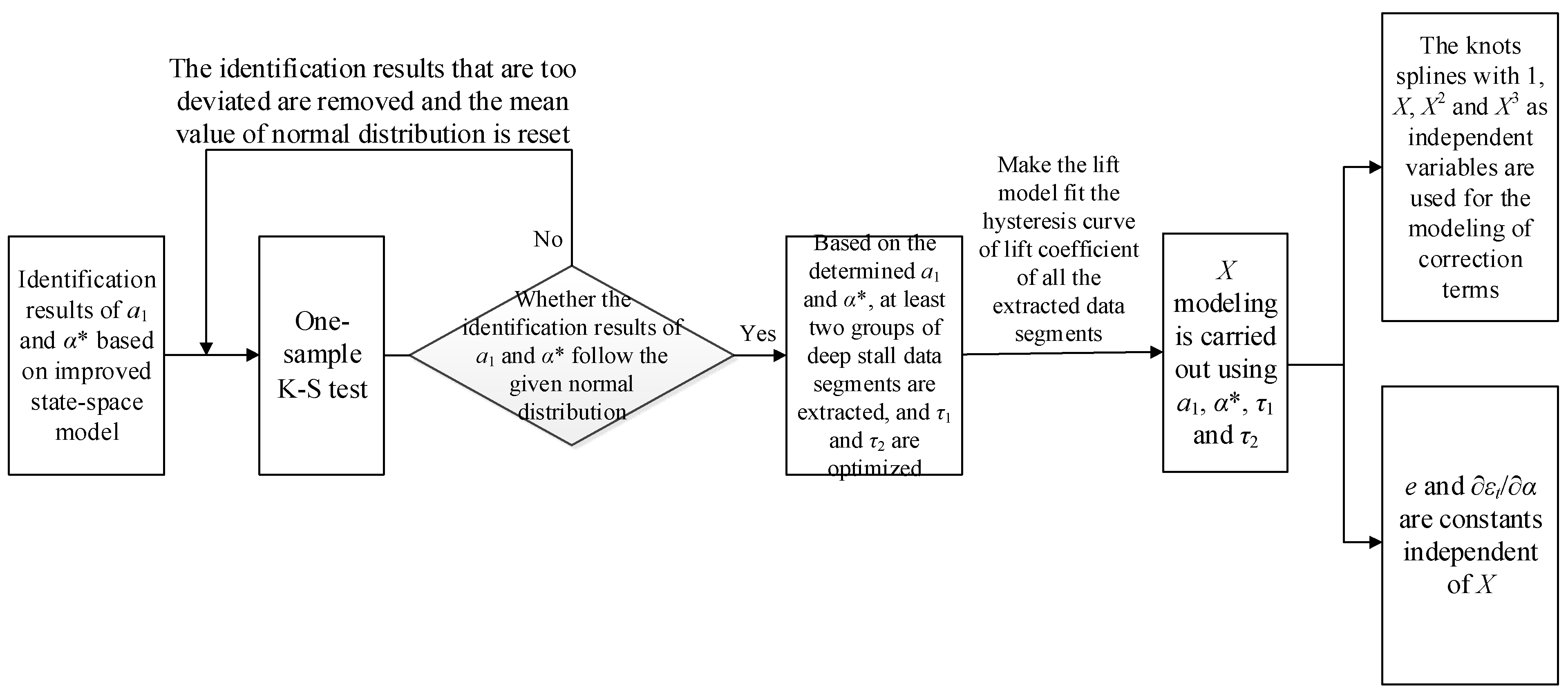
- a1 and α* are identified by the whole quasi-steady stall data. Then, it is checked whether the identification results of stall maneuver data with different stall degrees show normal distribution. If these identification results show the normal distribution, the values of a1 and α* are determined near the mean value of the normal distribution. If so, a1 and α* are taken as the mean of normal distribution. If the normal distribution is not followed, the identification results that are too discrete are eliminated and the mean value of the normal distribution is reset. The remaining identification results are tested to determine the values of a1 and α*.
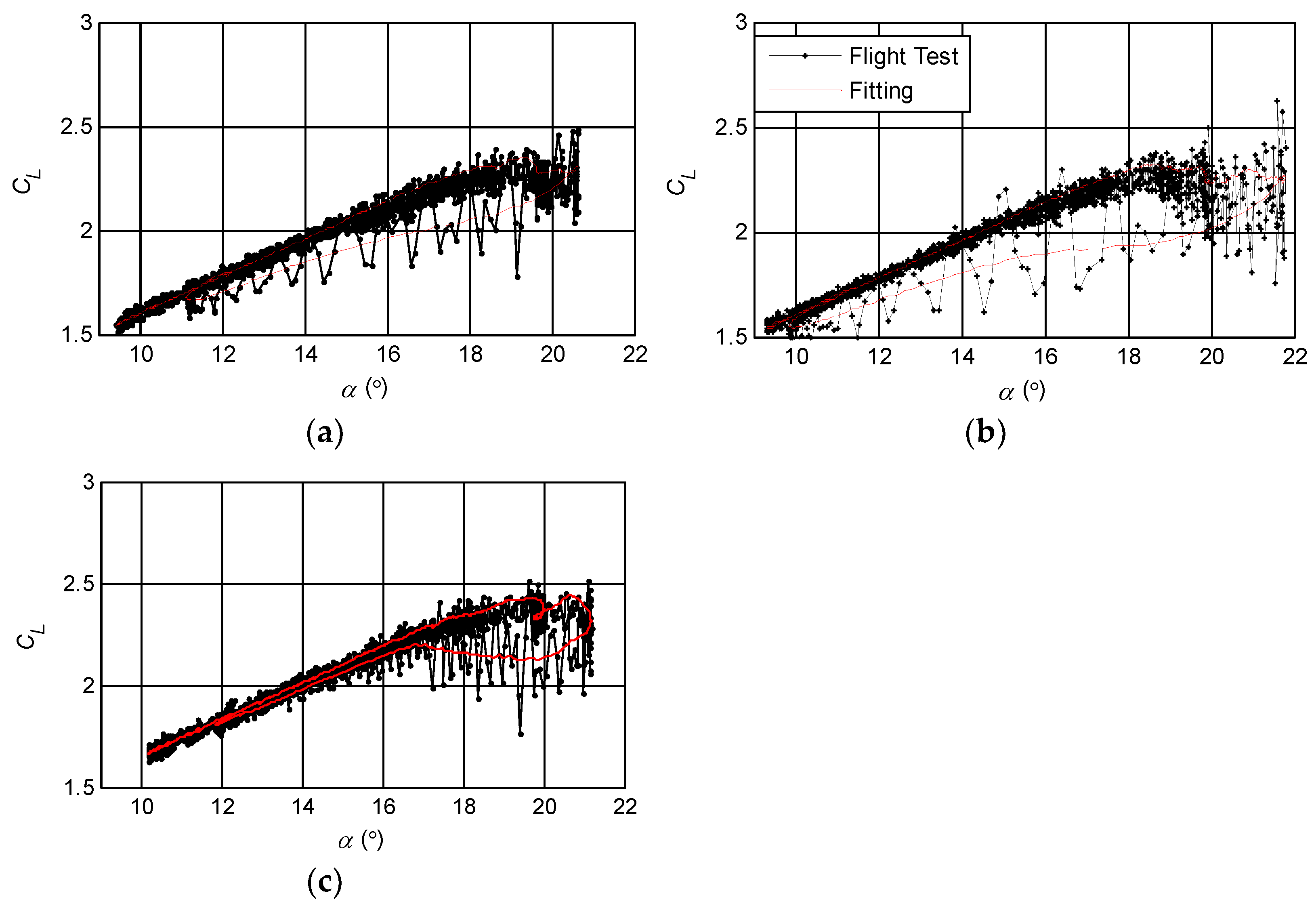
- The flight test data segments of at least two groups of aircraft from deep stall to stall recovery are extracted, and the τ1 and τ2 optimization are carried out to make the lift model fit all the extracted observation data segments well. Then, X modeling is carried out using a1, α*, τ1 and τ2.
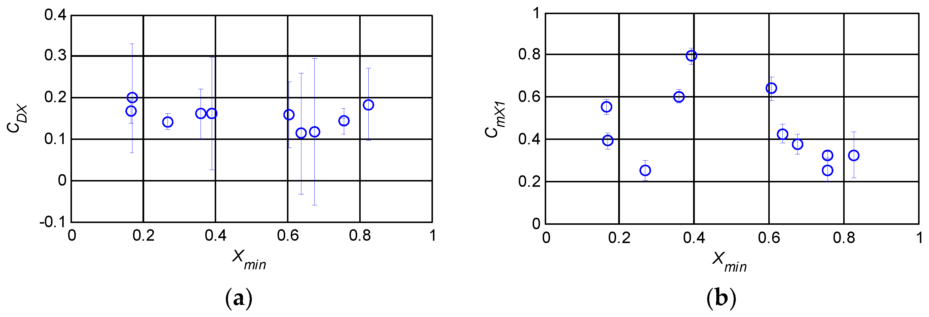
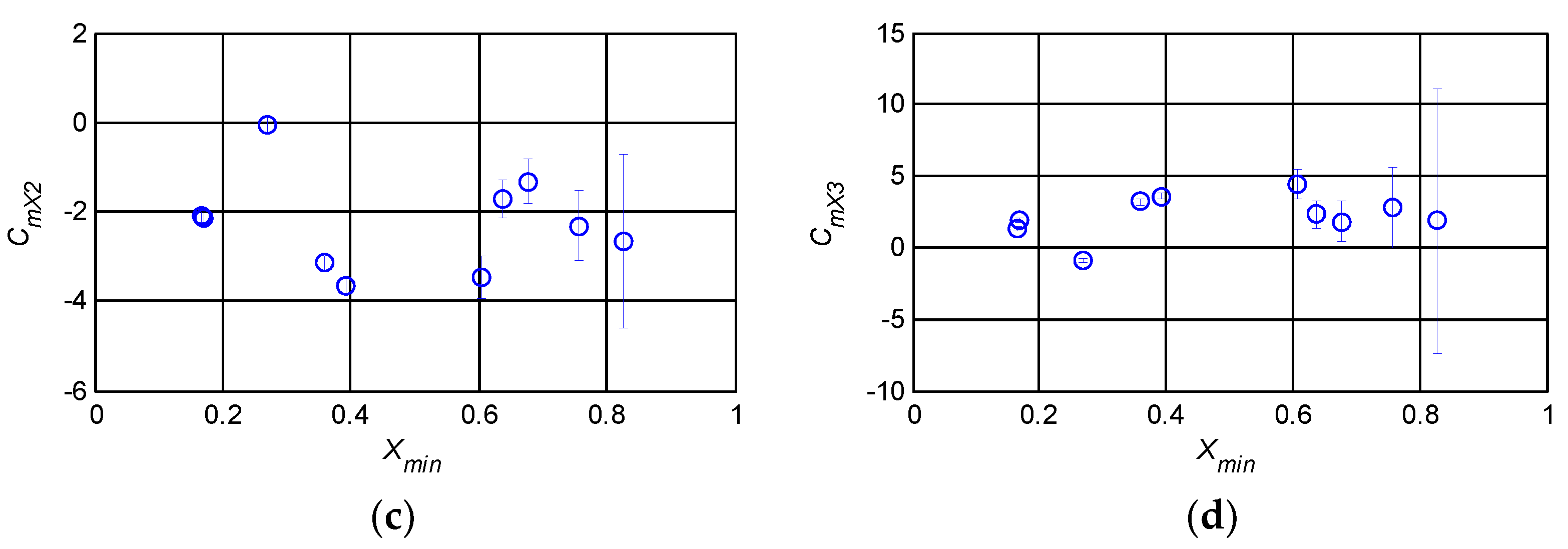
- After X modeling is completed, knots splines with 1, X, X2 and X3 as independent variables are used to carry out the modeling of CDX, CmX1, CmX2 and CmX3 under different stall degrees. e and ∂εt/∂α are determined as constants.
4. Stall Aerodynamic Parameter Identification and Modeling Example
4.1. Identification of Stall Aerodynamic Parameter
4.2. Aerodynamic Modeling of Stall Process
4.2.1. Modeling of X
4.2.2. Modeling of Correction Coefficient and e, ∂εt/∂α
- (1)
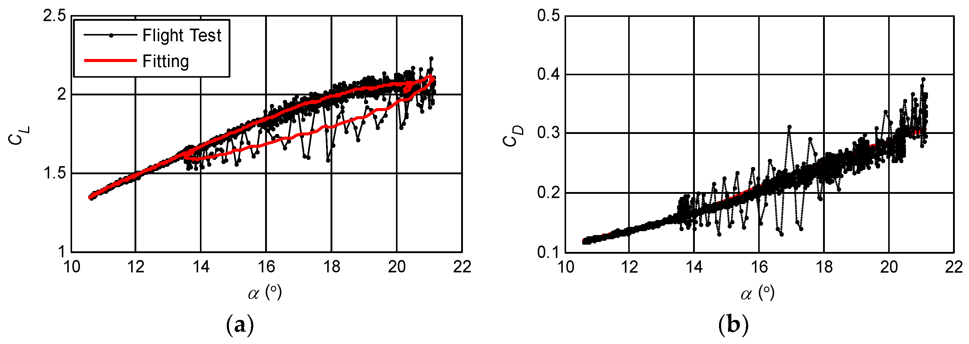
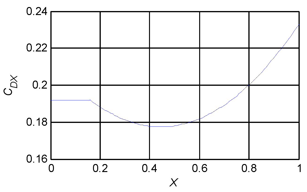
- CDX modeling
- (2)
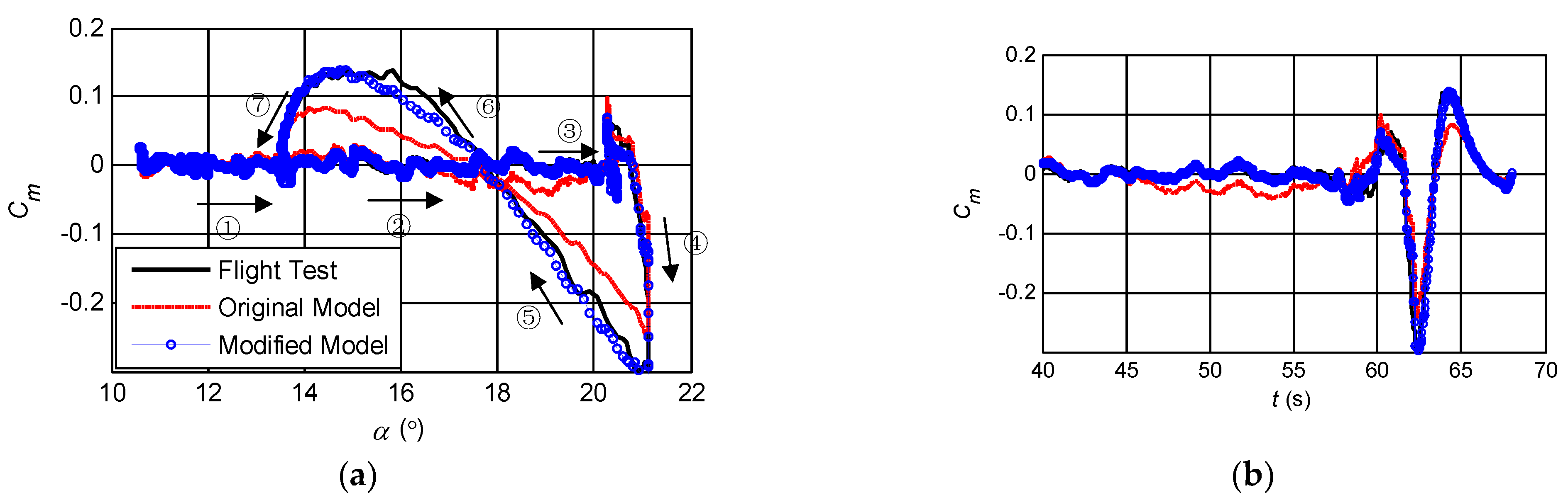
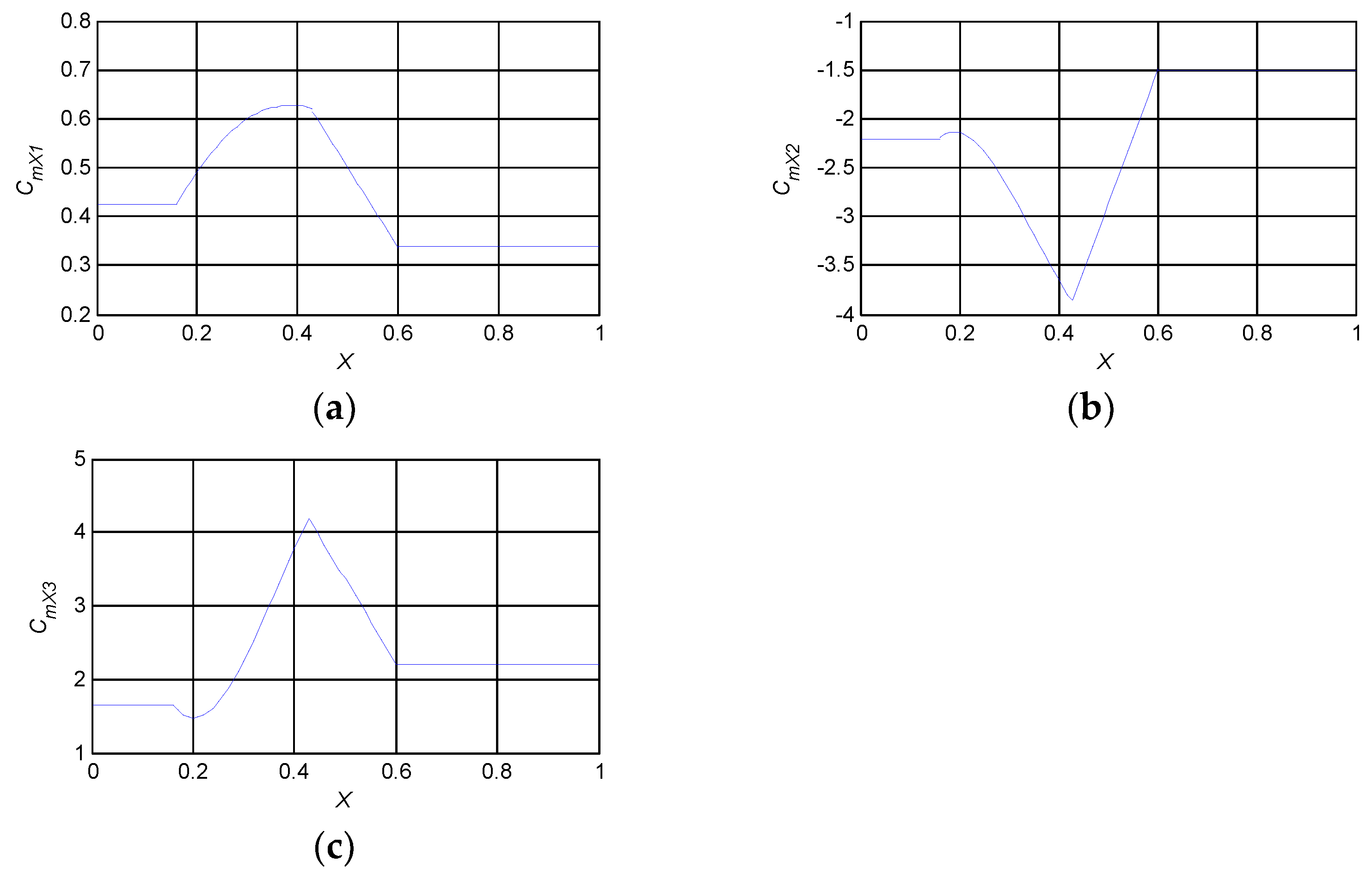
- Modeling of CmX1, CmX2 and CmX3
- (3)
- Modeling of e and ∂εt/∂α
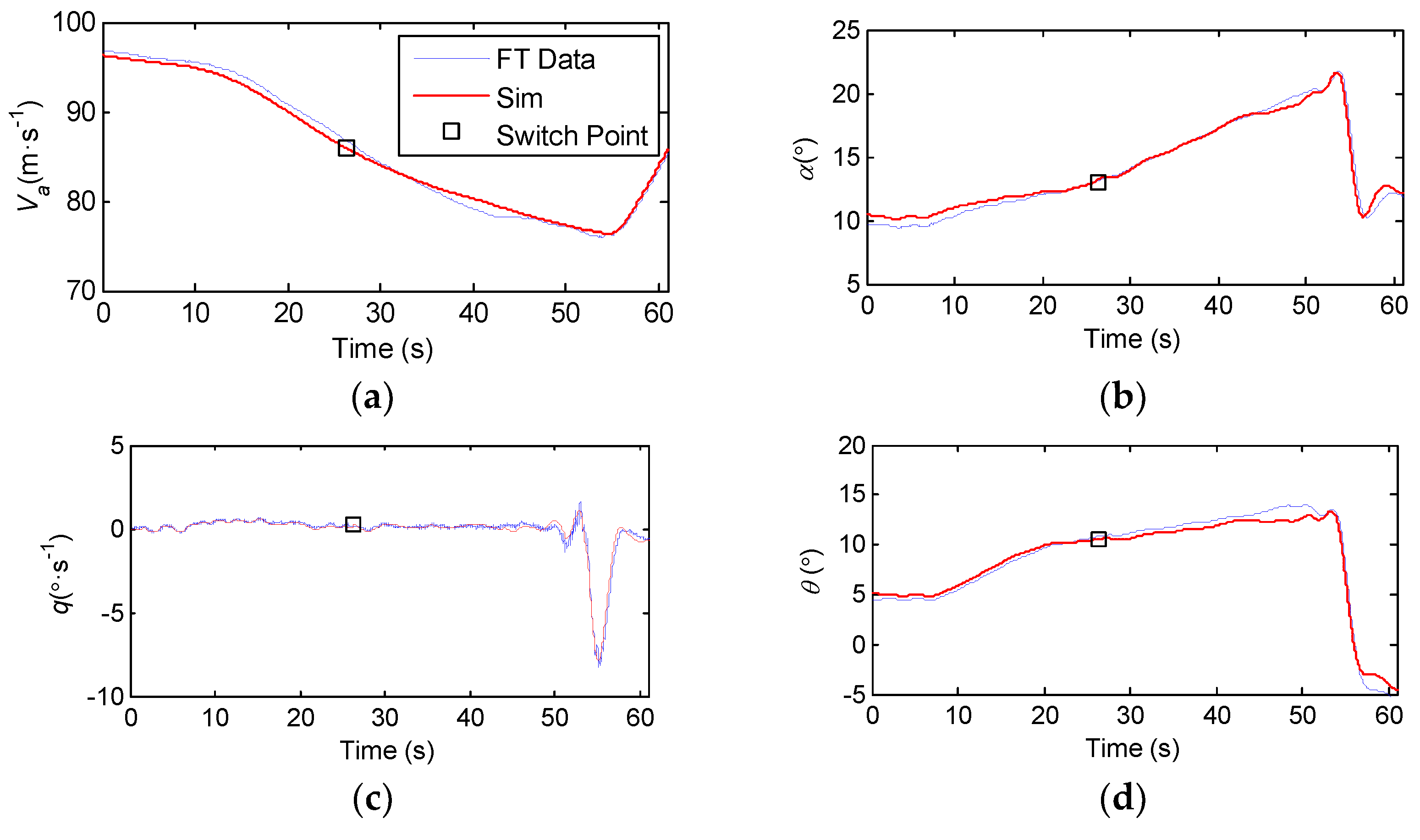
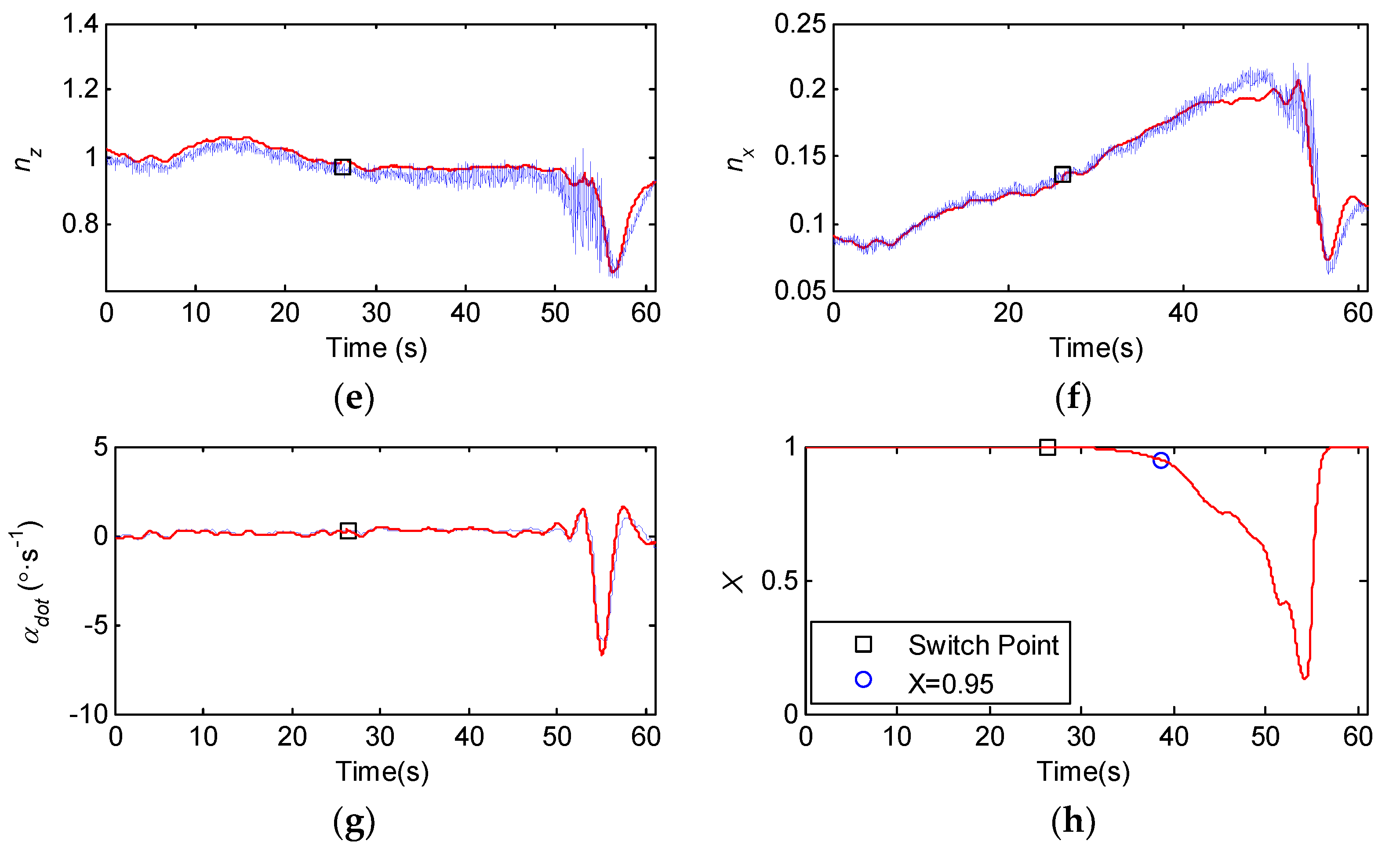
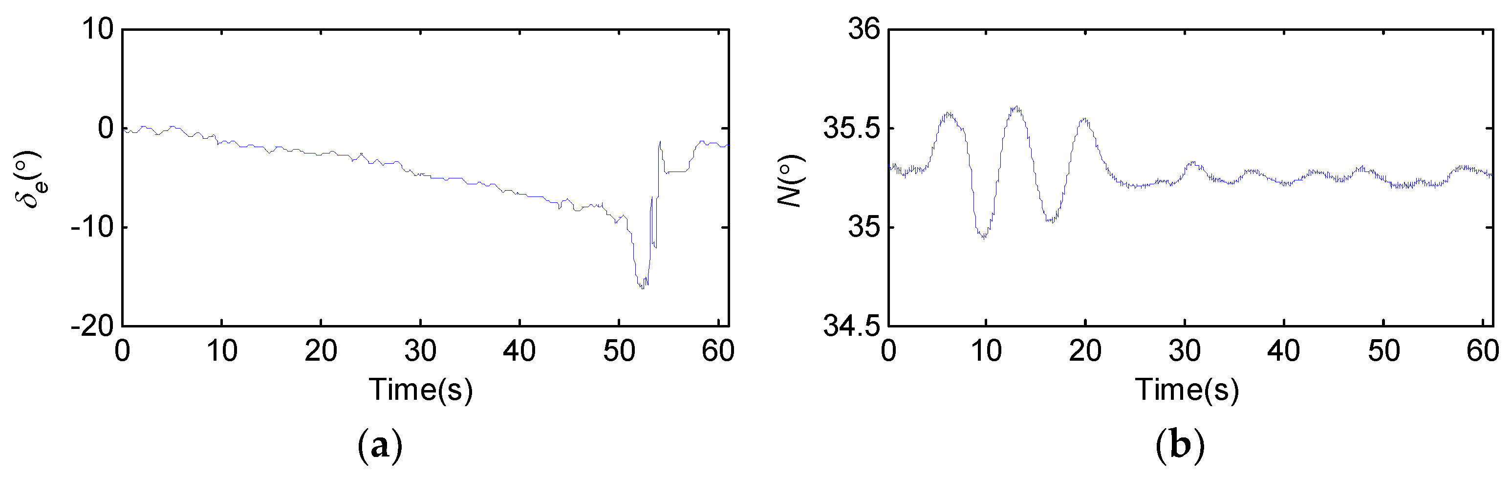
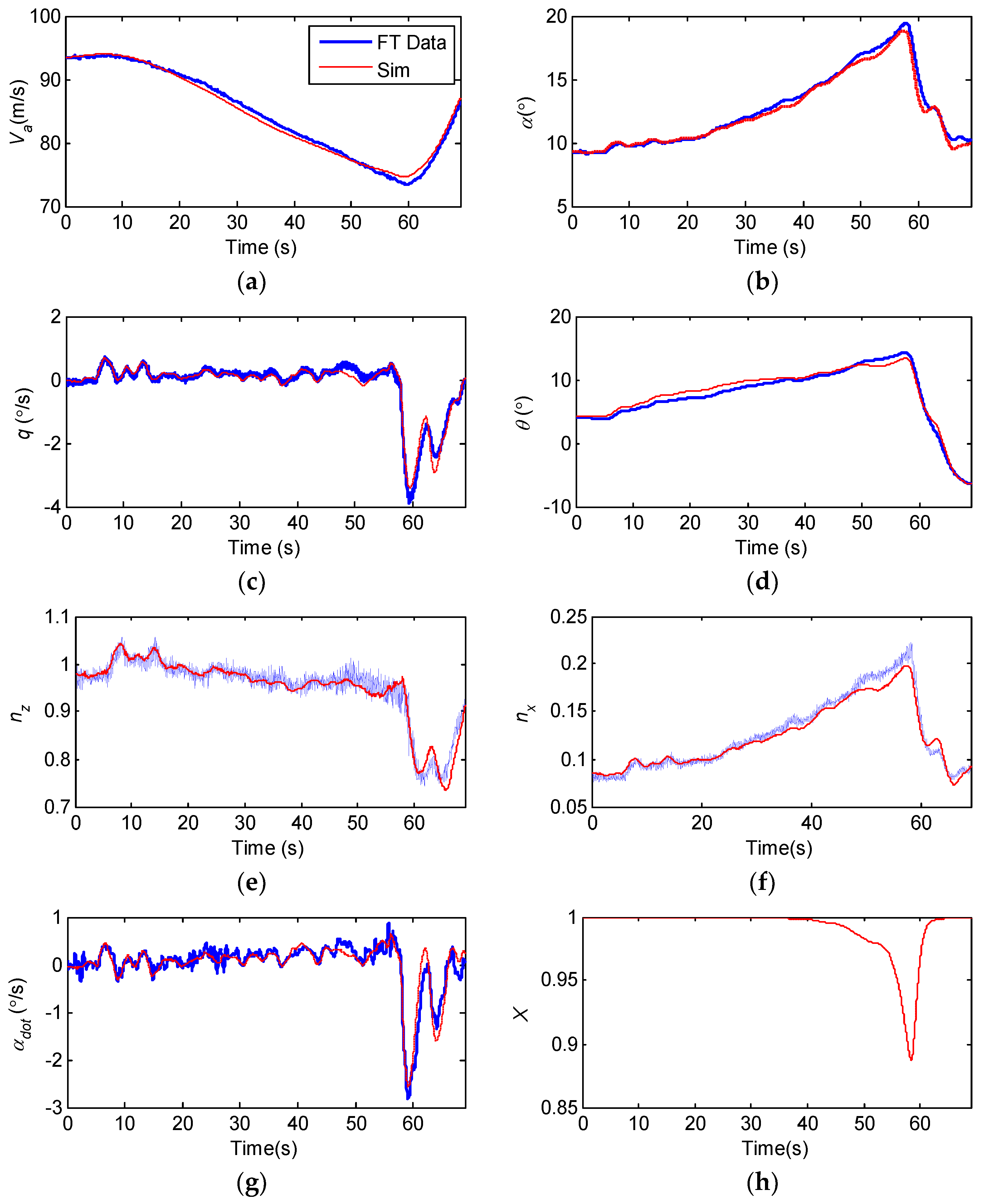
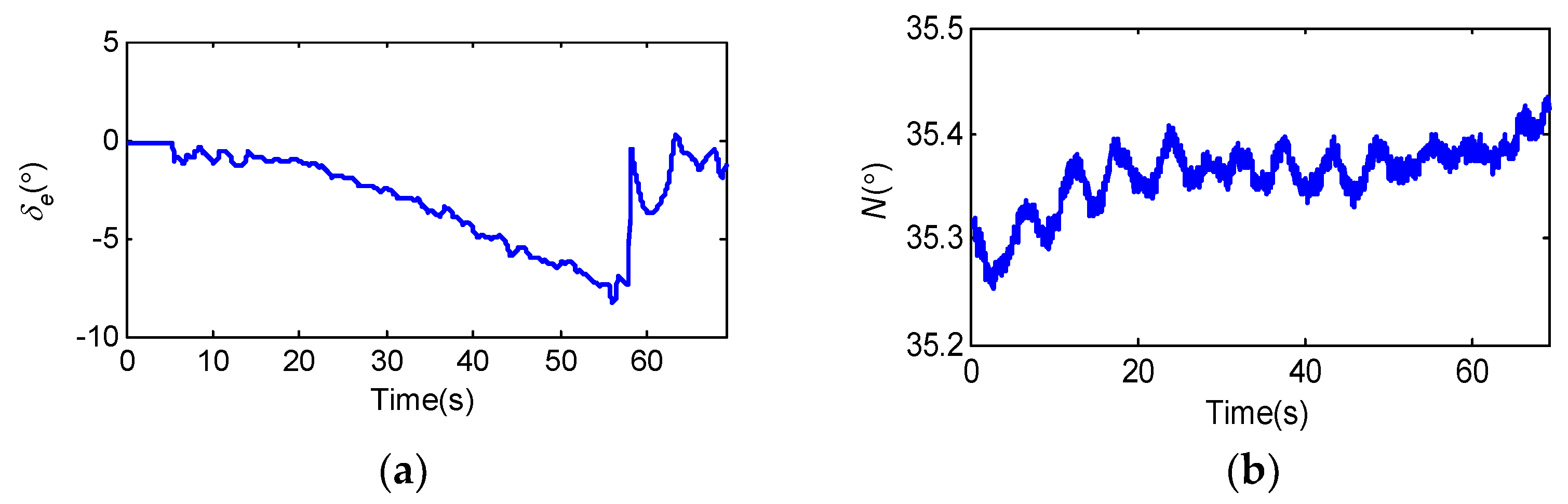
4.3. Mathematical Simulation Validation of Quasi-Steady Stall Flight
5. Conclusions
Author Contributions
Funding
Data Availability Statement
Conflicts of Interest
Notation
| AOA | angle of attack |
| MAC | mean aerodynamic chord |
| ODE | ordinary differential equation |
| DOF | degree of freedom |
| α | angle of attack (°) |
| V | airspeed (m/s) |
| q | pitch velocity (°/s) |
| dimensionless pitch velocity | |
| dimensionless change rate of AOA | |
| change rate of AOA (°/s2) | |
| dynamic pressure (Pa) | |
| S | reference wing area (m2) |
| wing area of horizontal tail (m2) | |
| mean aerodynamic chord length (m) | |
| δt | horizontal tail deflection angle (°) |
| δe | elevator deflection angle (°) |
| e | Oswald factor |
| Λ | aspect ratio |
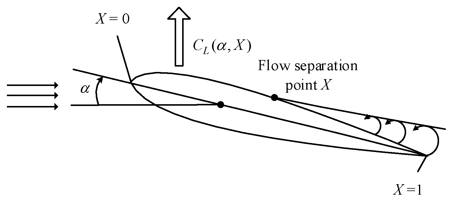
| X | relative position of the ideal flow separation point of the upper surface of the wing on the mean aerodynamic chord |
| αt | local AOA at horizontal tail (°) |
| εt | downwash angle at horizontal tail (°) |
| ε0 | downwash angle corresponding to zero lift AOA (°) |
| τ1 | time constant of unsteady separation process (/V) |
| τ2 | time constant of flow separation hysteresis (/V) |
| a1 | stall characteristics parameter of airfoil |
| α* | the AOA when flow separation point is equal to 0.5 (°) |
| ∂εt/∂α | derivative of downwash angle with respect to AOA |
| ∂εt/∂X | derivative of downwash angle with respect to X |
| CL | lift coefficient |
| CD | drag coefficient |
| Cm | pitching moment coefficient |
| CLαwb | lift curve slope of wing-body |
| CDX | empirical correction coefficient of drag |
| CmX | empirical correction coefficient of pitching moment |
| CmX1 CmX2 CmX3 | 1-order, 2-order, 3-order pitching moment correction term |
| Cmα | pitching static stability derivative |
| CLq | lift derivative due to pitching |
| lift derivative due to | |
| Cmq | pitching damping derivative |
| pitching damping derivative of lag of wash | |
| CLαt | lift derivative of horizontal tail |
| Cmδe | pitch control derivative of elevator |
| Cmδt | pitch control derivative of horizontal tail |
| Cmb | pitching moment coefficient of fuselage |
| Cmw0 | zero lift pitching moment coefficient of wing |
| CLw | lift coefficient of wing |
| Xw | the coordinate of wing pressure center relative to gravity center position in MAC fraction |
| lht | the distance from the aerodynamic center of the horizontal tail to the gravity center of the aircraft |
| Vt | local airspeed at horizontal tail |
| ax | longitudinal acceleration (m/s2) |
| T | thrust (N) |
| Ixx | moment of inertia with respect to roll axis (kg × m2) |
| Iyy | moment of inertia with respect to pitch axis (kg × m2) |
| Izz | moment of inertia with respect to yaw axis (kg × m2) |
| Ixz | product of inertia (kg × m2) |
Appendix A


References
- Jategaonkar, R.; Moennich, W. Identification of DO-328 aerodynamic database for a Level D flight simulator. In Proceedings of the Modeling and Simulation Technologies Conference, New Orleans, LA, USA, 11–13 August 1997. [Google Scholar]
- Gingras, D.R.; Ralston, J.N.; Oltman, R.; Wilkening, C.; Watts, R.; Derochers, P. Flight Simulator Augmentation for Stall and Upset Training. In Proceedings of the AIAA Modeling and Simulation Technologies Conference, National Harbor, MD, USA, 13–17 January 2014. [Google Scholar]
- Abramov, N.B.; Goman, M.; Khrabrov, A.N.; Soemarwoto, B.I. Aerodynamic Modeling for Poststall Flight Simulation of a Transport Airplane. J. Aircr. 2019, 56, 1427–1440. [Google Scholar] [CrossRef]
- Goman, M.; Khrabrov, A. Stall aerodynamic representation of aerodynamic characteristics of an aircraft at high angles of attack. J. Aircr. 1994, 31, 1109–1115. [Google Scholar] [CrossRef]
- Dias, N.J. Unsteady and Post-Stall Model Identification Using Dynamic Stall Maneuvers. In Proceedings of the AIAA Atmospheric Flight Mechanics Conference, Dallas, TX, USA, 22–26 June 2015. [Google Scholar]
- Dias, N.J.; Almeida, F.A. High Angle of Attack Model Identification Without Air Flow Angle Measurements. In Proceedings of the AIAA Atmospheric Flight Mechanics (AFM) Conference, Boston, MA, USA, 19–22 August 2013. [Google Scholar]
- Kumar, A.; Ghosh, A.K. GPR-based novel approach for non-linear aerodynamic modelling from flight data. Aeronaut. J. 2018, 123, 79–92. [Google Scholar] [CrossRef]
- Jategaonkar, R.V.; Fischenberg, D.; Von Gruenhagen, W. Aerodynamic Modeling and System Identification from Flight Data-Recent Applications at DLR. J. Aircr. 2004, 41, 681–691. [Google Scholar] [CrossRef]
- Ingen, J.V.; Visser, C.C.; Pool, D.M. Stall Model Identification of a Cessna Citation II from Flight Test Data Using Orthogonal Model Structure Selection. In Proceedings of the AIAA Scitech 2021 Forum, 11–15 & 19–21 January 2021. [Google Scholar] [CrossRef]
- Horssen, L.J.; Visser, C.C.; Pool, D.M. Aerodynamic Stall and Buffet Modeling for the Cessna Citation II Based on Flight Test Data. In Proceedings of the 2018 AIAA Modeling and Simulation Technologies Conference, Kissimmee, FL, USA, 8–12 January 2018. [Google Scholar]
- Liu, S.F.; Luo, Z.; Moszczynski, G.; Grant, P.R. Parameter Estimation for Extending Flight Models into Post-Stall Regime-Invited. In Proceedings of the AIAA Atmospheric Flight Mechanics Conference, San Diego, CA, USA, 4–8 January 2016. [Google Scholar]
- Teng, T.; Zhang, T.; Liu, S. Representative Post-Stall Modeling of T-tail Regional Jet and Turboprop Aircraft for Flight Training Simulator. In Proceedings of the AIAA Modeling and Simulation Technologies Conference, Kissimmee, FL, USA, 5–9 January 2015. [Google Scholar]
- Singh, J.; Jategaonkar, R. Flight determination of configurational effects on aircraft stall behavior. In Proceedings of the 21st Atmospheric Flight Mechanics Conference, San Diego, CA, USA, 29–31 July 1996. [Google Scholar]
- Nguyen, D.H.; Goman, M.; Lowenberg, M.H.; Neild, S.A. Evaluation of Unsteady Aerodynamic Effects in Stall Region for a T-Tail Transport Model. In Proceedings of the AIAA SCITECH 2022 Forum, San Diego, CA, USA & Virtual, 3–7 January 2022. [Google Scholar]
- Seo, G.-G.; Kim, Y.; Saderla, S. Kalman-filter based online system identification of fixed-wing aircraft in upset condition. Aerosp. Sci. Technol. 2019, 89, 307–317. [Google Scholar] [CrossRef]
- Dias, N.J. High Angle of Attack Model Identification with Compressibility Effects. In Proceedings of the AIAA Atmospheric Flight Mechanics Conference, Kissimmee, FL, USA, 5–9 January 2015. [Google Scholar]
- Saderla, S.; Dhayalan, R.; Ghosh, A. Non-linear aerodynamic modelling of unmanned cropped delta configuration from experimental data. Aeronaut. J. 2017, 121, 320–340. [Google Scholar] [CrossRef]
- Smets, S.C.; Visser, C.C.; Pool, D.M. Subjective Noticeability of Variations in Quasi-Steady Aerodynamic Stall Dynamics. In Proceedings of the AIAA Scitech 2019 Forum, San Diego, CA, USA, 7–11 January 2019. [Google Scholar]
- Grauer, J.A.; Morelli, E.A. Generic Global Aerodynamic Model for Aircraft. J. Aircr. 2015, 52, 13–20. [Google Scholar] [CrossRef]
- Morelli, E.A. Global nonlinear aerodynamic modeling using multivariate orthogonal functions. J. Aircr. 1995, 32, 270–277. [Google Scholar] [CrossRef]
- Brandon, J.M.; Morelli, E.A. Real-Time Onboard Global Nonlinear Aerodynamic Modeling from Flight Data. J. Aircr. 2016, 53, 1261–1297. [Google Scholar] [CrossRef] [Green Version]
- Boschetti, P.J.; Neves, C.; Ramirez, P.J. Nonlinear Aerodynamic Model in Dynamic Ground Effect at High Angles of Attack. In Proceedings of the AIAA SCITECH 2022 Forum, San Diego, CA, USA & Virtual, 3–7 January 2022. [Google Scholar]
- Morelli, E.A. Efficient Global Aerodynamic Modeling from Flight Data. In Proceedings of the 50th AIAA Aerospace Sciences Meeting Including the New Horizons Forum and Aerospace Exposition, Nashville, TN, USA, 9–12 January 2012. [Google Scholar]
- Morelli, E.A.; Cunningham, K.; Hill, M.A. Global Aerodynamic Modeling for Stall/Upset Recovery Training Using Efficient Piloted Flight Test Techniques. In Proceedings of the AIAA Modeling and Simulation Technologies (MST) Conference, Boston, MA, USA, 19–22 August 2013. [Google Scholar]
- Garcia, A.R.; Vos, R.; Visser, C. Aerodynamic Model Identification of the Flying V from Wind Tunnel Data. In Proceedings of the AIAA AVIATION 2020 FORUM, Virtual Event, 15–19 June 2020. [Google Scholar]
- Leung, J.M.; Moszczynski, G.J.; Grant, P.R. A State Estimation Approach for High Angle-of-Attack Parameter Estimation from Certification Flight Data. In Proceedings of the AIAA Scitech 2019 Forum, San Diego, CA, USA, 7–11 January 2019. [Google Scholar]
- Khrabrov, A.; Vinogradov, Y.; Abramov, N. Mathematical Modelling of Aircraft Unsteady Aerodynamics at High Incidence with Account of Wing-Tail Interaction. In Proceedings of the AIAA Atmospheric Flight Mechanics Conference and Exhibit, Providence, RI, USA, 16–19 August 2004. [Google Scholar]
- Fischenberg, D. Identification of an unsteady aerodynamic stall model from flight test data. In Proceedings of the 20th Atmospheric Flight Mechanics Conference, Baltimore, MD, USA, 7–10 August 1995. [Google Scholar]
- Imbrechts, A.; Visser, C.C.; Pool, D.M. Just Noticeable Differences for Variations in Quasi-Steady Stall Buffet Model Parameters. In Proceedings of the AIAA SCITECH 2022 Forum, San Diego, CA, USA & Virtual, 3–7 January 2022. [Google Scholar]
- Jategaonkar, R.V. Output Error Method. In Flight Vehicle System Identification: A Time Domain Methodology; AIAA: Reston, VA, USA, 2006; pp. 79–119. [Google Scholar]
- Luchtenburg, D.M.; Rowley, C.W.; Lohry, M.W.; Martinelli, L.; Stengel, R.F. Unsteady High-Angle-of-Attack Aerodynamic Models of a Generic Jet Transport. J. Aircr. 2015, 52, 890–895. [Google Scholar] [CrossRef] [Green Version]
- Klein, V.; Morelli, E.A. Data Analysis. In Aircraft System Identification—Theory and Practice; AIAA Education Series; AIAA: Reston, VA, USA, 2006; pp. 355–357. [Google Scholar]
- Federal Aviation Administration. Flight Training Device (FTD) Objective Tests. In CFR Part 60, Flight Simulation Training Device Initial and Continuing Qualification; Federal Aviation Administration: Washington, DC, USA, 2016; pp. 302–303. [Google Scholar]


| Number | αmax (°) | Xmin | a1 | s (a1) | α* (°) | s (α*) (°) | τ2 (c/V) | s (τ2) (c/V) | CDX | s (CDX) | CmX1 |
|---|---|---|---|---|---|---|---|---|---|---|---|
| 1 | 15.4 | 0.98 | 61.85 | 29.13 | 16.28 | 2.12 | 0.00 | 1156 | 1.08 | 0.0298 | 0.75 |
| 2 | 15.0 | 0.87 | 184.49 | 24.84 | 15.07 | 2.86 | −0.00 | 3517 | 0.25 | 0.0594 | 0.82 |
| 3 | 17.9 | 0.88 | 21.20 | 11.75 | 19.79 | 1.30 | −1.97 | 91.81 | 0.56 | 0.0046 | 0.33 |
| 4 | 17.0 | 0.95 | 33.88 | 13.69 | 17.82 | 2.44 | 2.18 | 377.8 | 0.69 | 0.0141 | 0.41 |
| 5 | 17.3 | 0.93 | 40.85 | 12.10 | 17.09 | 1.27 | −0.79 | 253.3 | 0.14 | 0.0155 | 0.32 |
| 6 | 18.8 | 0.75 | 22.87 | 12.11 | 20.11 | 0.64 | 2.18 | 16.93 | 0.14 | 0.0037 | 0.25 |
| 7 | 19.4 | 0.63 | 26.50 | 11.90 | 20.19 | 0.52 | 1.90 | 10.39 | 0.11 | 0.0731 | 0.42 |
| 8 | 19.3 | 0.67 | 29.56 | 12.14 | 20.09 | 0.75 | 0.00 | 13.29 | 0.12 | 0.0886 | 0.37 |
| 9 | 19.5 | 0.60 | 22.28 | 12.18 | 20.02 | 0.74 | 5.65 | 18.45 | 0.16 | 0.0399 | 0.63 |
| 10 | 18.5 | 0.82 | 17.37 | 10.62 | 20.46 | 0.23 | 2.24 | 11.80 | 0.18 | 0.0437 | 0.32 |
| 11 | 21.1 | 0.27 | 21.93 | 9.36 | 19.93 | 0.96 | 8.35 | 1.64 | 0.14 | 0.0092 | 0.25 |
| 12 | 20.6 | 0.39 | 19.56 | 8.11 | 20.07 | 0.87 | 4.85 | 3.07 | 0.16 | 0.0682 | 0.79 |
| 13 | 20.6 | 0.36 | 16.86 | 12.54 | 19.79 | 0.18 | 2.59 | 19.89 | 0.16 | 0.0309 | 0.60 |
| 14 | 21.7 | 0.16 | 27.33 | 8.73 | 19.78 | 0.38 | 3.28 | 0.30 | 0.17 | 0.0141 | 0.55 |
| 15 | 21.8 | 0.16 | 20.62 | 10.76 | 19.42 | 0.32 | 1.73 | 9.02 | 0.20 | 0.0655 | 0.39 |
| Number | s (CmX1) | CmX2 | s (CmX2) | CmX3 | s (CmX3) | e | s (e) | ∂εt/∂α | s (∂εt/∂α) | ||
| 1 | 0.021 | - | - | - | - | 0.81 | 0.046 | 0.385 | 0.002 | ||
| 2 | 0.026 | - | - | - | - | 0.80 | 0.017 | 0.36 | 0.002 | ||
| 3 | 0.009 | - | - | - | - | 0.81 | 0.016 | 0.35 | 0.002 | ||
| 4 | 0.009 | - | - | - | - | 0.81 | 0.026 | 0.36 | 0.002 | ||
| 5 | 0.009 | - | - | - | - | 0.79 | 0.022 | 0.40 | 0.002 | ||
| 6 | 0.028 | −2.32 | 0.39 | 2.81 | 1.38 | 0.79 | 0.011 | 0.40 | 0.001 | ||
| 7 | 0.023 | −1.71 | 0.21 | 2.32 | 0.49 | 0.81 | 0.016 | 0.38 | 0.001 | ||
| 8 | 0.024 | −1.33 | 0.25 | 1.83 | 0.67 | 0.80 | 0.012 | 0.38 | 0.001 | ||
| 9 | 0.027 | −3.48 | 0.24 | 4.49 | 0.52 | 0.83 | 0.014 | 0.36 | 0.002 | ||
| 10 | 0.055 | −2.67 | 0.97 | 1.85 | 4.65 | 0.80 | 0.011 | 0.40 | 0.003 | ||
| 11 | 0.023 | −0.06 | 0.086 | −0.91 | 0.086 | 0.77 | 0.009 | 0.37 | 0.001 | ||
| 12 | 0.019 | −3.66 | 0.087 | 3.57 | 0.110 | 0.78 | 0.017 | 0.37 | 0.001 | ||
| 13 | 0.017 | −3.15 | 0.080 | 3.17 | 0.100 | 0.79 | 0.011 | 0.34 | 0.003 | ||
| 14 | 0.018 | −2.10 | 0.061 | 1.35 | 0.055 | 0.80 | 0.008 | 0.36 | 0.001 | ||
| 15 | 0.020 | −2.16 | 0.073 | 1.85 | 0.069 | 0.78 | 0.011 | 0.34 | 0.002 |
Disclaimer/Publisher’s Note: The statements, opinions and data contained in all publications are solely those of the individual author(s) and contributor(s) and not of MDPI and/or the editor(s). MDPI and/or the editor(s) disclaim responsibility for any injury to people or property resulting from any ideas, methods, instructions or products referred to in the content. |
© 2023 by the authors. Licensee MDPI, Basel, Switzerland. This article is an open access article distributed under the terms and conditions of the Creative Commons Attribution (CC BY) license (https://creativecommons.org/licenses/by/4.0/).
Share and Cite
Wang, L.; Zhao, R.; Xu, K.; Zhang, Y.; Yue, T. Identification and Modeling Method of Longitudinal Stall Aerodynamic Parameters of Civil Aircraft Based on Improved Kirchhoff Stall Aerodynamic Model. Aerospace 2023, 10, 333. https://doi.org/10.3390/aerospace10040333
Wang L, Zhao R, Xu K, Zhang Y, Yue T. Identification and Modeling Method of Longitudinal Stall Aerodynamic Parameters of Civil Aircraft Based on Improved Kirchhoff Stall Aerodynamic Model. Aerospace. 2023; 10(4):333. https://doi.org/10.3390/aerospace10040333
Chicago/Turabian StyleWang, Lixin, Rong Zhao, Ke Xu, Yi Zhang, and Ting Yue. 2023. "Identification and Modeling Method of Longitudinal Stall Aerodynamic Parameters of Civil Aircraft Based on Improved Kirchhoff Stall Aerodynamic Model" Aerospace 10, no. 4: 333. https://doi.org/10.3390/aerospace10040333