Article

Adjoint-Based Aerodynamic Design Optimization and Drag Reduction Analysis of a Military Transport Aircraft Afterbody

1
Aeronautics Faculty, Northwestern Polytechnical University, Xi’an 710072, China
2
Aeronautics Faculty, Xi’an Jiaotong University, Xi’an 710049, China
3
Computational Aerodynamics Institute, China Aerodynamics Research and Development Center, Mianyang 621000, China
*
Author to whom correspondence should be addressed.
These authors contributed equally to this work.
Aerospace 2023, 10(4), 331; https://doi.org/10.3390/aerospace10040331
Submission received: 14 February 2023 / Revised: 10 March 2023 / Accepted: 15 March 2023 / Published: 27 March 2023
(This article belongs to the Special Issue Adjoint Method for Aerodynamic Design and Other Applications in CFD)

Abstract

:
Based on the adjoint method, the afterbody of a military transport aircraft was optimized and designed to meet engineering constraints under real flight conditions. Guidance for the key design parameters of the afterbody of the military transport aircraft is given. The vortex dynamics and boundary layer extraction methods were used to analyze the optimization results of military transport aircraft. It was found that, upstream of the vortex shedding point, the circumferential accumulation process of the vorticity is weakened. The position of the vortex shedding and the appearance of the saddle line are delayed by reducing the circumferential inverse pressure gradient and the intensity of the crossflow. The afterbody vortex system of the optimized configuration is further away from the surface. Meanwhile, the distance between the counter-rotated vortex decreases, and the upwashing speed of the vortex core is smaller. Therefore, vortex-induced drag is reduced. Finally, compared with the initial configuration, the optimized configuration has a relative drag reduction of 23.2%.

1. Introduction

To satisfy the requirements of a modern military transport aircraft for loading and unloading cargo while reducing the landing and take-off angle of attack and avoiding collisions with the ground, the afterbody is usually designed as an upswept stern. The upswept angle causes crossflow on the afterbody and increases the lateral inverse pressure gradient [1]. Since the afterbody is located downstream from the region where the boundary layer develops on the whole aircraft, a vortex-dominated separated flow appears, and this eventually leads to the formation of two counter-rotating vortices [2]. This vortex pair creates a low-pressure region, which increases the cruise drag of the aircraft [3]. Due to the afterbody, the drag is about one-third of the total drag of the transport [4]. At the same time, for military transport aircraft, the vortices not only increase the cruise drag but also result in an upwash toward the centerline of the afterbody, which may interfere with airdrop missions [5]. Therefore, it is necessary to carry out design optimization research on the afterbody of the transport aircraft.
In recent years, due to the increase in the missions of long-range transport aircraft, this problem has received more attention. Studying the influence of body shape on flow characteristics has great significance in theory and engineering. This is the key technology of the vehicle body design. Statistical results show that the drag of the fuselage could be reduced by about 0.5–3% if the shape of the afterbody is well designed. Remarkable economic benefits can be achieved [6].

1.1. Related Works

Many scholars have conducted research on the flow mechanism of the afterbody. Morel (1980) [7] reported that there are two typical separation patterns, which can be defined as quasi-axisymmetric separation patterns and three-dimensional separation patterns. Maull (1980) [8] found that a high drag is associated with the formation of strong longitudinal vortices in the wake and can be sensitive to the experimental configuration, for instance, the slant angle. The same phenomenon was observed by Xia and Bearman (1983) [9], and Britcher and Alcorn [10] (1991) used slanted base cylindrical models and reported that the strength of wake vortices is influenced by the state of the forebody boundary layer. Epstein (1994) [2] concluded that the structure of the afterbody vortex was only weakly dependent on the Reynolds number. Bulathsinghala (2017) [11] studied the time-average and unsteady phenomenon of the afterbody vortex with an upswept angle from 24° to 32° by the PIV experiment. Their study found that the drag coefficient is proportional to the circulation, and the circulation will gradually increase as the upswept angle increases. In the unsteady state, for all upswept angles, in the flow to the trailing edge, the vortices gradually form coherence, the radius of the vortex core decreases, and the meandering amplitude decreases. Wang (2017, 2018) [12,13] pointed out three phases and two patterns in the interaction of the vortex system of the afterbody with a horizontal tail. The result quantitatively reveals the internal connection between the circulation, the vortex center trajectory, and the vortex-induced drag, which can be mainly used for the generation mechanism of the vortex drag. Based on the vorticity moment theorem (VMT), the vorticity loop model was proposed to explain the physical and mathematical meaning of a vortex drag. The model can accurately calculate the vortex-induced drag for a three-dimensional steady or unsteady vortex system. Garmann (2019) [14] conducted numerical simulations and experiments to investigate the flow transition characteristics and the instability of the detached vortex of the afterbody configuration with an upswept angle of 28° where M = 0.1 . Ranjan [15,16] observed and characterized vortex meandering or wandering by performing large eddy simulations (LESs) of the flow behind an axisymmetric slanted base configuration. The meanderings of these vortices were analyzed by proper orthogonal decomposition (POD) and the linear stability theory (LST) at the downstream position. A complete experimental reconstruction of the three-dimensional mean flow field of a cylinder with an inclined base was carried out by Zigunov (2020) [17] to reveal the complex details of the flow. A schematic diagram of the flow characteristics of a typical bluff body was given, and the common flow characteristics of the vortex-dominated wake flow of a cylinder with a slanted base were summarized. Shi [18] demonstrated the behavior of several turbulence models on the vortex shedding phenomena. In Cravero’s study [19], a method was proposed to describe and estimate the recirculating length behind an aerodynamic profile with a Gurney flap in the ground effect. In addition, Chen et al. [20] studied the interaction mechanism between the sweeping jet and the afterbody vortex system.
Unfortunately, the flight conditions for all the studies mentioned above are low-speed and have small Reynolds numbers, and there are few studies on the flow of the upswept afterbody under high-speed cruise conditions. A recent study showed that compressibility is a crucial factor to change the wake of the afterbody [21]. The configuration used is a simplified configuration with a slanted base, which fails to factually characterize the surface of the afterbody. Different shapes of the edge can form different mean flow topologies, and this will result in the changed upstream boundary layer evolution, which has an effect on the wake of the afterbody [22]. So far, there have been few studies on the upstream formation of the afterbody detached vortex and its relationship with the characteristics of the boundary layer.
The detached vortex system is studied especially for military transport aircraft afterbodies considering the influence of the cargo bay. Johnson (2002) [23] used PIV experiments and computational fluid dynamics (CFD)-based numerical simulations to study the afterbody flow of the C-130 military transport aircraft when the tailgate was open. Both experiments and numerical simulations showed the same phenomenon and trend. There are spanwise and longitudinal vortices below the afterbody surface and consistent upward flow in the cargo bay. Bury (2008, 2013) [5,24] experimentally studied the afterbody vortex flow of a simplified C-130 military transport aircraft with a ratio of 1:16. The complex vortex dynamics under the closed and opened cargo door configurations are respectively revealed, as is the strong interaction between the afterbody surface and vortex. Bergeron (2009) [25] used the PIV experiments, the numerical delayed detached-eddy simulation (DDES) method, and the detached-eddy simulation (DES) method to study the unsteady flow of the afterbody of the C-130 military transport aircraft in closed and open door configurations. Based on the preliminary studies of unsteady flow in open door configurations, spiral and shedding instabilities have been quantified for future verification with experimental data.
The upswept angle, contraction ratio, fineness, and flatness are several key design parameters in the shape design of the afterbody. Kolesar (1983) [26] experimentally studied the influence of the parameters of the afterbody and obtained the influence rules of various parameters. He also established a database and developed an engineering method for predicting the drag of the afterbody. Subsequent researchers studied the influence and sensitivity of afterbody design parameters through calculation and experimental methods and obtained many useful conclusions. Studies by Kong (2002, 2003) [27,28] have shown that the main mechanism of the drag of the afterbody lies in the existence of a larger contraction ratio and upswept angle structure, which leads to the generation of separation vortices. The geometric parameter that has the greatest influence on the afterbody is the contraction ratio, followed by the upswept angle [29]. Zhang (2004) [30] used the fluorescence and the laser light sheet method in the water channel to study different afterbodies of an airliner. The study showed that there are two different types of wake vortices: the stable wake vortex and the periodically shedding wake vortex chain. When the contraction ratio of the afterbody increases, periodic fluctuations occur. This situation also occurs when there is interference from the tail. Zhang (2010) [4] constructed three types of large upswept afterbody models using three typical transport aircraft as prototypes. CFD methods were used to study the drag and flow characteristics of the three fuselages. This study introduced a new afterbody design parameter—near-roundness—and proved that near-roundness and its changes along the axis of the fuselage better describe the influence of the afterbody section shape on the pressure drag. The pressure drag is the decisive factor in the change of the afterbody drag, although it only accounts for 15–20% of the total drag of the fuselage. Reducing the contraction ratio and the upswept angle can both reduce the pressure drag. When the upswept angle and fineness are similar, the flatness is the main factor affecting the pressure drag. Whether the transition between the side and bottom of the afterbody is gentle or not is one of the main factors affecting flow separation [31]. In the research process of this article, these key design parameters (upswept angle, contraction ratio, fineness, flatness, and near-roundness) will be combined to analyze the optimized design results.
To reduce the drag of the afterbody, many efforts have been made focusing on two aspects: the vortex flow control of the afterbody and the afterbody design optimization. Although the vortex generator can effectively reduce the drag of the afterbody, the parasitic drag it causes will also reduce the drag reduction benefits, resulting in a drag reduction of only 5% or less. Active flow control has a better drag reduction effect, but it also has the phenomenon that the required external power may be greater than the power saved due to drag reduction. Therefore, the direct design optimization of the afterbody surface needs further study.
Regarding the design optimization of the afterbody, major airlines have made many successful attempts to improve the economic efficiency of operations. For example, the MD-80 aircraft reduced the cruise drag coefficient by 0.5% to 1.0% after redesigning the afterbody. The Airbus company adopted a wide-body fuselage with a large upswept angle and contraction ratio for the first time in the development of the Airbus A-300. With this optimized design, the afterbody drag was significantly reduced. Wang (2013) [32] carried out an aerodynamic design optimization on the C17 military transport aircraft under engineering constraints. Under the condition that the maximum width, height, and upswept angle of the afterbody are not reduced, the cruise pressure drag after the optimization can be reduced by 19.8%, and the total drag can be reduced by 2.6%. The flow pattern analysis shows that the main reasons for the reduction in the drag of the optimized afterbody are the increase in the near-roundness of the afterbody section and the decrease in the change of the near-roundness along the axis of the fuselage, which reduce the circumferential inverse pressure gradient of the afterbody. Yang (2014) [33] established a design optimization system that involves the free-formed deformation (FFD) parameterization method, the radial basis function (RBF) dynamic mesh method, the Kriging surrogate model, and an improved differential evolution algorithm. The design optimization system was used in afterbody drag reduction in consideration of the interference of engines. The optimization result showed that the total drag reduces by 2.67%, which is a benefit from the change in the flow tube shape between the afterbody and the nacelle. Bai (2015) [6] used the FFD parameterization method coupled with the Kriging surrogate model and a quantum particle swarm algorithm to establish the aerodynamic design optimization framework. By reducing the pressure recovery gradient, the drag coefficient decreases by six counts, and the lift–drag ratio increases by 3%. From the above research and practice, it can be seen that the optimized design of the afterbody can play an important role in the drag reduction design of the large upswept afterbody of a large transport aircraft. It can be expected to be more effective for drag reduction after the design optimization of the afterbody.
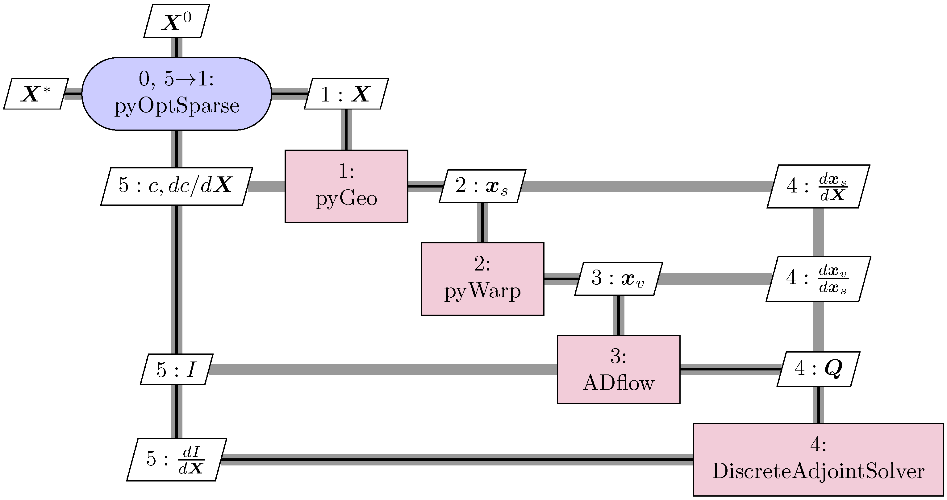
The design optimization based on the adjoint theory is relatively mature, and there are a variety of solvers. The ADflow [34] solver is an efficient and reliable solver based on Reynolds-averaged Navier–Stokes (RANS) equation that couples discrete adjoint equations, which can be used to solve structured mesh and overset mesh. Kenway [35] made a detailed evaluation of the accuracy, efficiency, and scalability of the ADflow program for solving the adjoint equations. Considering the computational efficiency and engineering practicability, we chose the gradient optimization method based on ADflow.

1.2. State of the Art

In conclusion, many studies have been carried out on the problems of transport aircraft afterbody flow separation and vortex-induced drag. These studies focus on the flow mechanism of the upswept afterbody, the rule of parameter influence, and the application of drag reduction measures. There are many research results that have been applied to engineering practice. At present, the drag reduction design of the afterbody mainly focuses on afterbody vortex flow control. However, due to the influence of parasitic drag and the power consumption caused by flow control, the net drag reduction effect is greatly reduced. Therefore, a direct design optimization of the afterbody surface still has an advantage. On the one hand, most of the currently published design optimization studies use non-gradient algorithms. When large-scale design variables are involved, the dimensional curse will occur, and non-gradient algorithms are not as practical and efficient as gradient optimization algorithms for engineering problems. On the other hand, the design optimization mentioned above only pursues the effect of drag reduction without an in-depth analysis of the cause and mechanism. Previous studies on afterbody vortices have focused on the evolution and wandering of the vortex core after vortex shedding. Few studies have been carried out on the upstream formation of the vortex and boundary layer characteristics of the afterbody before the vortex detached point.
Therefore, the main purpose of this paper is to apply the adjoint-based gradient optimization algorithm to a drag reduction design optimization, which satisfies the engineering constraints of the upswept afterbody of military transport aircraft, and to conduct a detailed analysis of the reasons for drag reduction by vortex dynamics and boundary layer extraction.

2. Geometry and Grid

2.1. Afterbody Design Parameters

The upswept angle β , contraction ratio ζ , fineness λ , flatness W, and near-roundness ϕ are several key design parameters in the shape design of the afterbody. The upswept angle of the afterbody is defined as the angle between the horizontal line and the line connecting the center of the maximum section of the afterbody and the center of the 95% length section. The fineness ratio of the afterbody is defined as the ratio of the length of the afterbody to the maximum diameter of the afterbody. The contraction ratio of the afterbody is defined as the ratio of the cross-sectional diameter d B of 95% of the length of the afterbody to the maximum diameter d A . The detailed definition of parameters is shown in Figure 1.
The flatness of the afterbody is defined as W = ( 2 h B ) w , as shown in Figure 2, where h B and w are, respectively, the distance between the zero longitudinal down point of a certain normal section of the afterbody and the maximum width point and the maximum width of the section. The smaller the flatness is, the flatter the cross-section is.
The definition of near-roundness is shown in Figure 2 below. It is defined as the closeness of the cross-section shape to the reference circle whose diameter is the distance between the upper and lower zero longitudinal points on a certain normal section, namely ϕ = R / R m a x . Among them, R is half of the distance between the upper and lower zero longitudinal points, i.e., the radius of the reference circle of the normal section; R m a x is the distance from the farthest point of the section to the center of the reference circle. The closer ϕ is to 1, the higher the degree of the near circle.

2.2. Model and Grid Generation

We created a simplified model of military transport aircraft with only the fuselage for aerodynamic design optimization. The aircraft’s initial configuration is based on the C-130 military transport plane. To ensure the axisymmetric surface symmetry of the fuselage and the smooth continuity of the left and right half models during the design optimization, the model was chosen for each. The parameters of the military transport model are shown in Table 1. Figure 3 depicts three views of the model.
The commercial software ANSYS-ICEM is used to divide the surface of the fuselage into a multi-block structured grid, and the spatial O-shaped topology grid is generated by the program p y h y p (https://github.com/mdolab/pyhyp accessed on 24 October 2019).

2.3. Grid Sensitivity

We used the overset mesh for the simulations, as shown in Figure 4. A grid convergence study was carried out to determine the resolution accuracy of this grid. In order to consistently describe the findings of grid convergence research, Roache [36,37] proposes the grid convergence index (GCI). Two levels of the grid can be used to compute the GCI; however, three levels are advised to precisely estimate the order of convergence and verify that the solutions are contained within the asymptotic range of convergence. There are three levels of the grid in our study, named L2, L1, and L0.5. The GCI between L1 and L0.5 is defined as:
GCI L 1 L 0.5 = F s | ε | r g q 1
where ε is the relative error between the two grids. r g is the refinement ratio, which is approximately 1.2 in our case, and q is the order of convergence. F s is the safety factor. Additionally, the GCI between L2 and L1 is defined as:
GCI L 2 L 1 = F s | ε | r g q r g q 1
The amount of mesh and the corresponding drag coefficients and GCIs are shown in Table 2, where a converged trend can be seen. Each grid level must produce solutions that fall within the computed solution’s asymptotic range of convergence. Two GCI values computed over three grids can be used to verify this, as shown in Equation (3):
GCI L 1 L 0.5 = r g q GCI L 2 L 1 10.497 1 . 2 2.6 × 6.384
We can see that the L1 mesh has sufficient accuracy. Choosing the L1 level as an example which was also applied in the optimization design, the minimum quality is 0.39, and the minimum volume is 6.8 × 10 9 . Taking 50 times the length of the fuselage, it is a spherical far field. The height of the first layer is smaller than 1 × 10 6 m, aiming to set the desired y + below 0.5. The zoom figure of the grid around the wall of the afterbody and fuselage nose is shown in Figure 5.

3. CFD Simulation Method and Validation

We use open-source numerical simulation software ADflow to calculate the flow solution. The flow control equations are three-dimensional compressible steady Reynolds-averaged Navier–Stokes (RANS) equations in an integral form, as shown in Equation (4).
Q t + 1 V F I · d S 1 V F V · d S = 0
where Q represents the conserved variables, V is the control volume, and S is the surface of the control volume. F I and F V are, respectively, the inviscid flux term and the viscous flux term.
In this paper, the Spalart-Allmaras (SA) one-equation turbulence model is used [38]. The calculation accuracy and calculation efficiency of this equation are high, and the simulation result of typical subsonic and supersonic flows is good; it is suitable for engineering a numerical simulation and an aerodynamic optimization design.
The explicit central difference finite volume method proposed by Jameson et al. [39] is currently one of the main calculation methods in the field of CFD. It uses a semi-discrete method to completely separate the integration of spatial discrete and time advancement. Using this semi-discrete method to discretize the governing equation Equation (4), we can get
d V i , j , k Q i , j , k d t + A F I i , j , k + A F V i , j , k = 0
Q i , j , k are the conserved variables at a given grid cell, and V i , j , k correspond to the volume of the grid cell. A F I i , j , k and A F V i , j , k are the inviscid and viscous fluxes of the grid cell, respectively.
To ensure the numerical stability of the central difference scheme, the second-order central scheme needs to introduce artificial viscosity D i , j , k . In the ADflow solver, the total fluxes can be expressed by
A F i , j , k = A F I i , j , k + A F V i , j , k D i , j , k
The semi-discrete form of the general governing equation Equation (4) can be further expressed as
d V i , j , k Q i , j , k d t + A F i , j , k = 0
For steady flow, the flux of a conserved variable in a given unit is 0, that is, there is a residual equation
A ( Q ) = 0
For the time advance method, the current commonly used algorithms of the ADflow solver are primarily: coupling RK (Runge–Kutta) [39] or D3ADI (diagonalized diagonally dominant alternating direction implicit) [40] and the NK (fully Newton–Krylov) algorithm [41], or coupling ANK (an approximate Newton–Krylov) [42] and the NK (fully Newton–Krylov) algorithm. The iteration will continue only until the total residual error in the flow field drops by ten orders of magnitude.
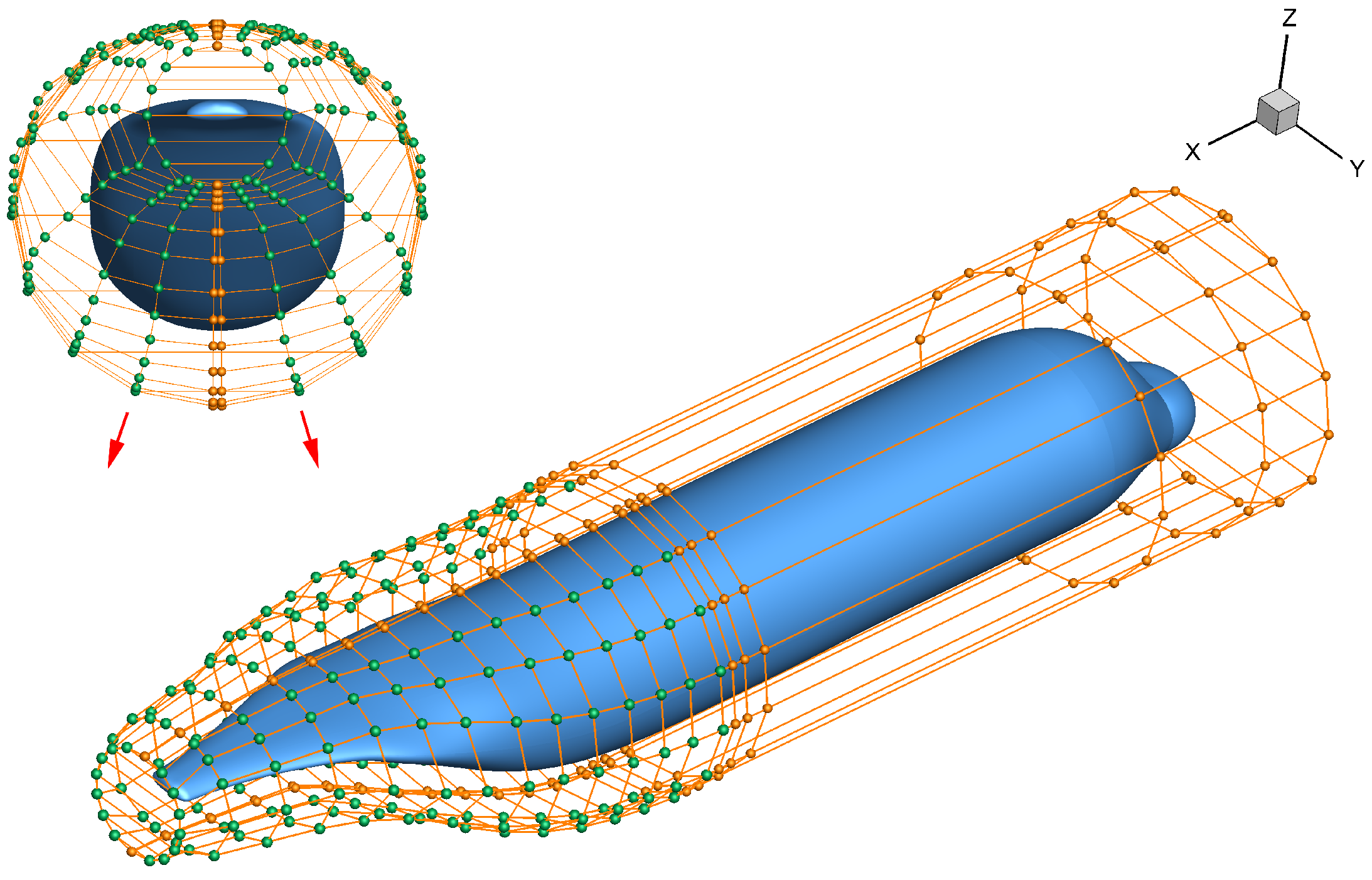
The accuracy of the solver is verified using the configuration of the common research model (CRM). The calculation status is M = 0.85 , C l = 0.5 , R e = 5 × 10 6 . The mesh is shown in Figure 6, and the total amount of mesh is 10.8 million. 
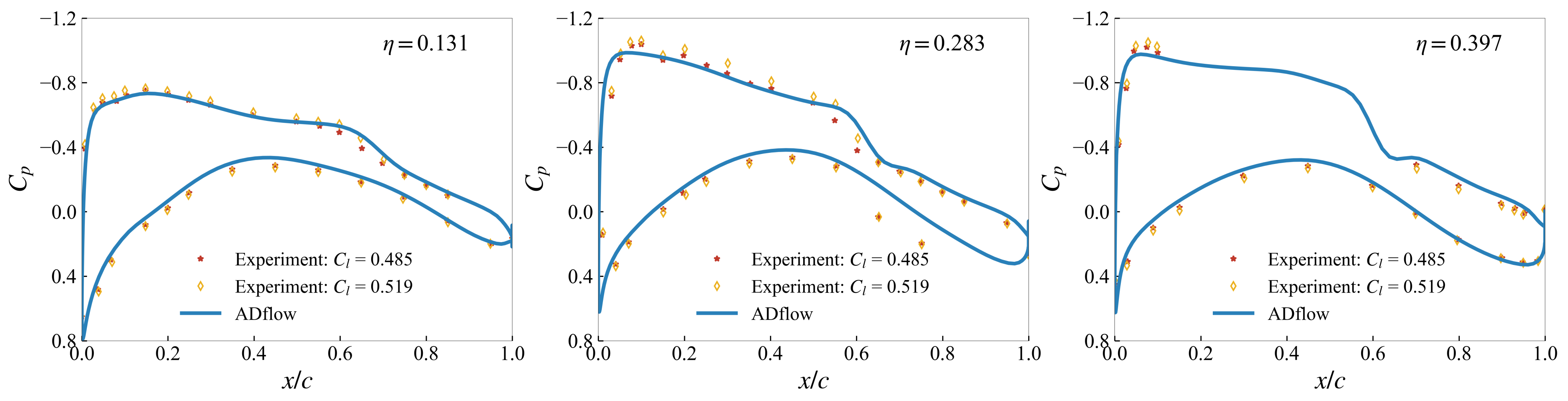
Figure 7 compares the ADflow solution and the experimental pressure distributions for these profiles. The states corresponding to the test are M = 0.85 , C l = 0.485 , R e = 5 × 10 6 and M = 0.85 , C l = 0.519 , R e = 5 × 10 6 . Figure 7 shows that the experiment and the numerical pressure distributions are in good agreement. The data of the lower airfoil basically coincide, and the upper airfoil has obvious differences at the leading edge and the shock wave capture. The reasons for these differences may be model manufacture error and aeroelastic deformation.

4. Optimization Framework

Our work is based on an open-source optimization framework called MACH-Aero. The flow solver in this framework is ADflow, which can automatically differentiate the RANS flow solution Q by adjoint equations. The partial derivatives are solved by the reverse AD method with Tapenade [43] in Jacobi-free form. The Newton–Krylov solution method based on the general minimum residual (GMRES) was used to solve adjoint equations [42].
We created mathematical mappings of the design variables X and geometric shapes x s in MACH-Aero by using the FFD parameterization tool p y G e o (https://github.com/mdolab/pygeo (accessed on 24 October 2019)). A useful tool for mesh warping in MACH-Aero is I D w a r p (https://github.com/mdolab/idwarp (accessed on 24 October 2019)), which establishes the mapping between the spatial x v and surface grids x s . The design optimization of the afterbody in this study was processed using the SNOPT algorithm, which is based on the sequential quadratic programming (SQP) algorithm and is part of the p y O p t S p a r s e (https://github.com/mdolab/pyoptsparse (accessed on 24 October 2019)) module, due to its evident efficiency advantage. The entire design optimization framework is shown in Figure 8, where the objective function is defined as I, and the constraints are represented as c. When the optimization is converged, we can obtain the optimal design variables X * .

5. Analysis Method of Afterbody Vortex System

5.1. Boundary Layer Extraction from RANS Solutions

In order to explore the relationship between the boundary layer and the afterbody’s counter-rotated vortex system, the boundary layer of the fuselage was extracted from the RANS solutions. The flow profiles inside the boundary layer may be directly separated from the flow fields obtained by the structured-grid flow solver ADflow. The profile range in the normal direction is determined by the boundary layer thickness ( δ e ). More precisely, δ e is defined as that distance above the wall where u = 0.99 u e ; here, u e is the velocity at the outer edge of the boundary layer. The number of streamlines to extract profiles is determined by the resolution of the grid in the RANS solutions.
The characteristic quantities of the boundary layer that we are concerned with include the displacement thickness of the boundary layer and the momentum thickness of the boundary layer.
δ 1 = 0 y 1 1 ρ u ρ e u e d y δ e y 1
δ 2 = 0 y 1 ρ u ρ e u e 1 u u e d y δ e y 1
The displacement thickness ( δ 1 ), which is defined as Equation (9), reflects the real inviscid boundary of the wall, and a thin boundary layer displacement thickness will reduce the pressure drag. On the other hand, the momentum thickness ( δ 2 ), as expressed in Equation (10), is an index that is proportional to the decrement in momentum flow due to the presence of the boundary layer. It is the height of a hypothetical stream tube carrying the missing momentum flow at freestream conditions. In more detailed discussions of boundary layer theory, it can be shown that δ 2 evaluated at a given station x = x 1 is proportional to the integrated friction drag coefficient from the leading edge to x 1 , i.e., Equation (11).
δ 2 x 1 1 x 1 0 x 1 c f d x = C f

5.2. Vortex-Tracking Method

Based on the mean velocity fields obtained from CFD, the vortex structures that develop in the afterbody can be identified using the Q criterion [44].
Assume the deformation tensor is u . The Q criterion can be calculated by
Q = 1 2 Ω 2 S 2
where the vorticity tensor Ω = 0.5 u + u T and the strain tensor S = 0.5 u u T are, respectively, symmetrical and asymmetrical components. A positive value of Q represents the regions in which the rotation exceeds the strain and will be identified as a vortex. The vortex center is located at the position of the maximum Q value.
We define the circulation Γ to assess the vortex strength,
Γ = Σ ω x d y d z
The non-dimensional circulation can be expressed by
Γ ¯ = Γ U D
where D is the diameter of the afterbody section along the flow direction. Here, each circulation is averaged by two counter-rotating vortices.
In order to track the interesting movements of the vortex pairs, the coordinates of the vortex center are calculated by weighting the vorticity distribution within a core:
y c = 1 Γ Σ y ω x d y d z
z c = 1 Γ Σ z ω x d y d z
Once the vortex center is obtained, the circulation of this center is then calculated using an area integral of vorticity before expanding the area by one spatial grid resolution unit each time and recalculating the circulation until the residuals between iterations are less than 1%.

5.3. The Vorticity Loop Model and Vortex-Induced Force

Studies [13] have shown that the wake vortex structure of a clean fuselage afterbody configuration can be represented by a single-vortex loop model, as shown in Figure 9.
For a single-vortex loop model, the vortex-induced drag only depends on the longitudinal vortex wash. In a single-vortex loop model, due to the self-induction of the vortex loop points to the vertical direction, the lateral vortex wash only exists during the rolling up of the shear layer at the trailing edge of the wing or the bottom of the afterbody. For a solid in a sufficiently large enclosed control volume R v , assuming its relative air movement, based on the vorticity moment theorem (VMT) [45], the aerodynamic force acting on it is the area occupied by the solid and its surrounding fluid, which are R s and R f , respectively.
F = ρ 2 d d t R v r × ω d R + ρ d d t R v v d R
where r is the position vector pointing to the fluid element from the origin, and w is the vorticity vector of the fluid element.
The second term of Equation (17) is zero since we focus on a rigid body with a non-rotating solid-wall boundary moving forward at a constant velocity in a viscous flow. Therefore, the aerodynamic force can be rewritten as
F = ρ 2 d d t R v r × ω d R
The vortex-induced force in Equation (18) can be projected to the x axis corresponding to the afterbody drag direction. According to AMT theory, the afterbody drag is highly related to the bending of the vortex tube along the y and z directions in the crossflow wake plane.
F x = ρ 2 d d t R v ( y ω z z ω y ) d R
Based on Stoke’s formula, circulation is the vortex current flowing through the vortex tube section.
S v ω · n S v d S = Γ v
where S v is the section of vortex tube, and n S v represents the normal vector of the section. Therefore, the volume integral of Equation (18) can be converted into the surface integral of the vorticity and the line integral of the position vector along the circumference.
F = ρ 2 d d t l r × S v c ω d S d l = ρ 2 d d t l r × d l Γ v
According to the Green theorem, the aerodynamic force in Equation (21) is projected in the arbitrary direction n, which is based on the right-hand side. It becomes
l r × d l · n = 2 d A p · n = 2 A p n
where A n denotes the projection area of a vorticity loop in the n direction. Hence, the vortex force in the n direction is
F = F · n = ρ d d t A n Γ v
To satisfy the Helmholtz theorem, Equation (23) is simplified as follows:
F = F · n = ρ d A n d t Γ v
For a single-vortex loop model, the center of the vortex loop will only move in the vertical direction in the three-dimensional enclosed area, and its enclosed area is shown in Figure 9.
d A x = b r , 0 d y
Hence, the time-average force generated by a single-vortex loop model can be described as
D ¯ v = ρ u v w Γ v b r , 0 L ¯ v = ρ U Γ v b r , 0
where b r , 0 is the center distance of two counter-rotating wake vortex tubes, and u v w is the vortex wash speed in the vertical direction produced by the self-induction of the vorticity loop.

6. Optimization Problem

For military transport aircraft, we define the optimization problem by Equation (27):
min C D s . t . β β V afterbody 0.9 V afterbody
where β is the upswept angle of the afterbody, and V afterbody is the volume of the afterbody capacity. The flow condition is M = 0.57 , α = 2 . 5 , R e = 7.46 × 10 6 . Considering the actual needs of the engineering, the optimization constraints are set such that the upswept angle is not reduced, and the volume of the optimization result is not less than 90% of the initial volume.
As shown in Figure 10 and Figure 11, the FFD control frame contains 20 sections, and 12 sections have been chosen to monitor the section shape. All sections are within the length of the fuselage. Detailed information on these 12 sections is shown in Table 3. All movable FFD control points are selected in these 12 sections. Twenty points are arranged in each section, maintaining symmetry on the left and right. To ensure symmetry during deformation, the two rows of points close to the plane of symmetry are restrained from moving, and the left and right points move symmetrically during the deformation process. At the same time, considering the upswept angle constraint, the final design variable number is 106.

7. Optimization Results

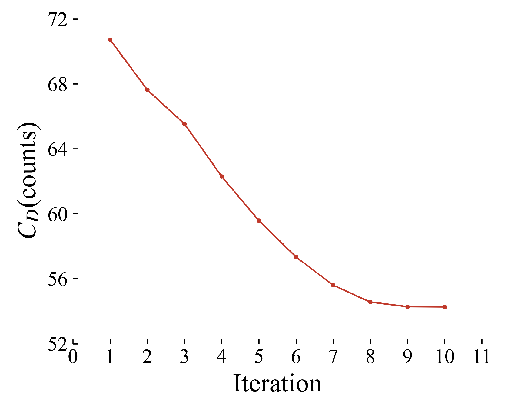
The history of optimization is shown in Figure 12, which converged in 10 major iterations. The comparison of the drag coefficient before and after optimization is shown in 
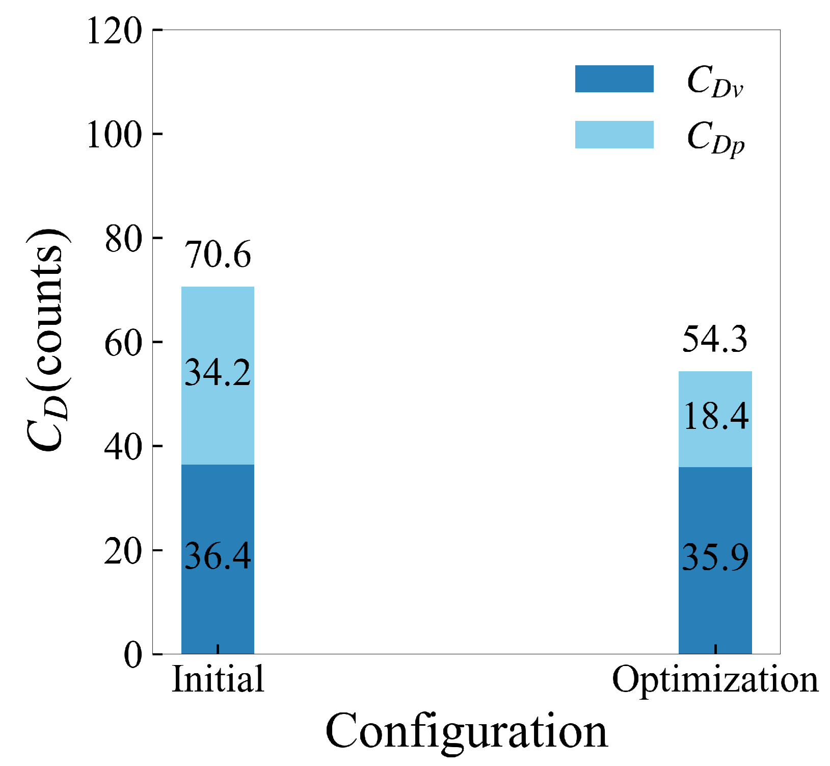
Table 4. After optimization, the drag is reduced by 16.4 counts, and the relative drag reduction can reach 23.2%. The decomposition of drag is shown in Figure 13, where the viscous drag changes from 36.4 counts before optimization to 35.9 counts after optimization, which is a small change; on the other hand, the pressure drag is greatly reduced from 34.2 counts to 18.4 counts. From the perspective of drag decomposition, the optimization mainly reduces the total drag by reducing the pressure drag, which includes the vortex-induced drag caused by the detached vortex wake.
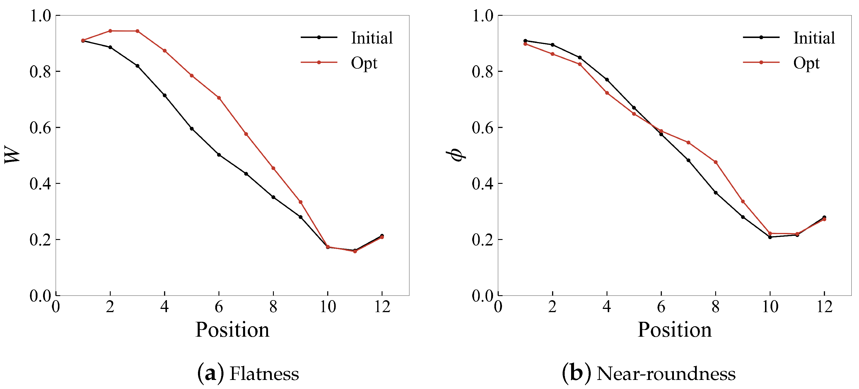
The flatness and near-roundness changes of military transport aircraft optimization are shown in Figure 14. Regarding the flatness, the optimized configuration is higher than the initial configuration overall, indicating that the optimized direction makes each section fuller rather than flatter. Compared to the initial configuration, the optimized result only has greater near-roundness in the sixth to tenth cross-sections while, in other positions, it is basically equivalent to the initial configuration or even reduced. However, it is worth noting that the change in the near-roundness along the axis of the fuselage is slower through the optimization.
The comparison of afterbody surfaces before and after the military transport aircraft optimization is shown in Figure 15 below. From the side view, compared with the initial configuration, the front of the afterbody protrudes upwards from the top of the fuselage and shrinks upwards at the bottom, which tends to increase the upswept angle. This phenomenon contradicts the previous conclusion that the higher the angle is, the greater the drag is. At the same time, it is interesting that, from the top view, the surface of this part of the optimized configuration is narrowed on the left and right sides of the fuselage, forming a shape similar to a “bee waist”. In the middle of the afterbody, the optimized configuration keeps the left and right widths equivalent to the initial configuration while widening in the vertical direction. There is almost no change in the tail of the afterbody.
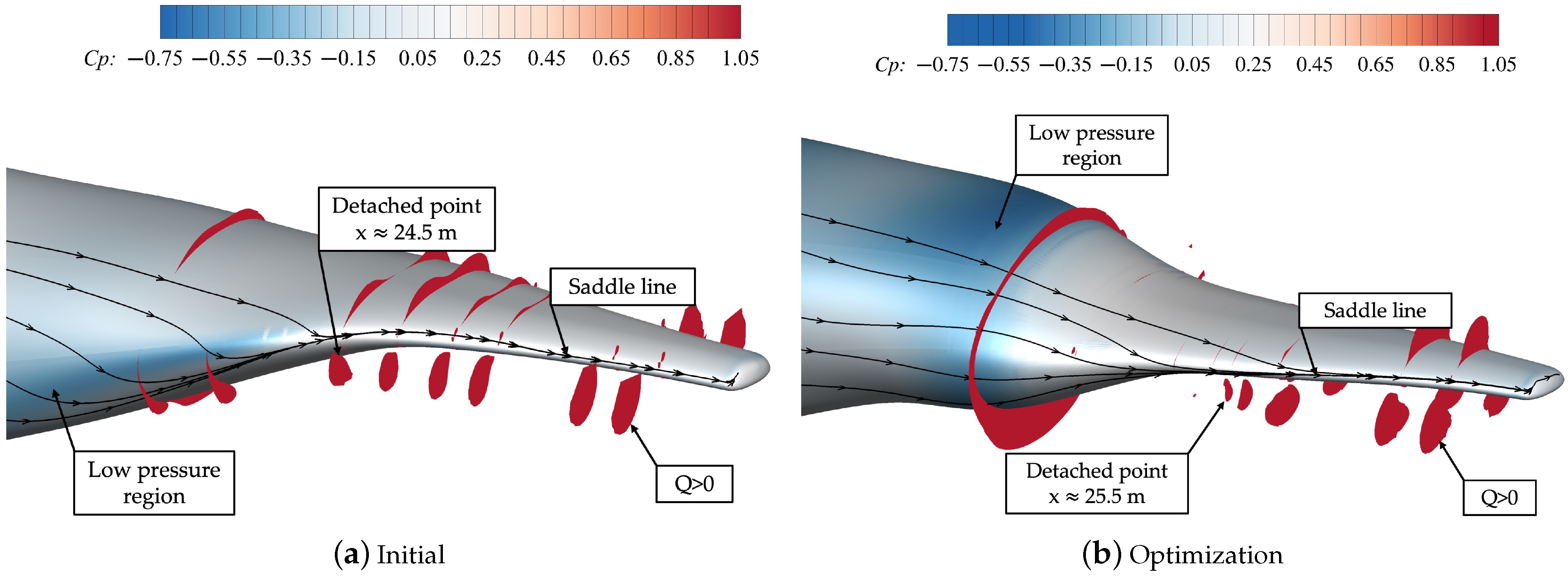
Figure 16 shows the surface pressure coefficient contour. The surface streamlines the distribution of the initial configuration and the optimized configuration. The red patches in the space are the vortex structure extracted by the Q criterion ( Q > 0 ) in the flow field. Both the initial configuration and the optimized configuration have a low-pressure region on the surface. The difference is that the optimized configuration has a more uniform circumferential pressure distribution on the fuselage surface and a smaller circumferential pressure gradient than the initial configuration. Due to the existence of the circumferential pressure gradient of the fuselage, the two configurations have different degrees of crossflow, and the streamlines appear to have an overly obvious convergence (i.e., saddle lines [17]) and finally lead to the appearance of a detachment vortex footprint. The optimized configuration delays the detached point by approximately 1 m.
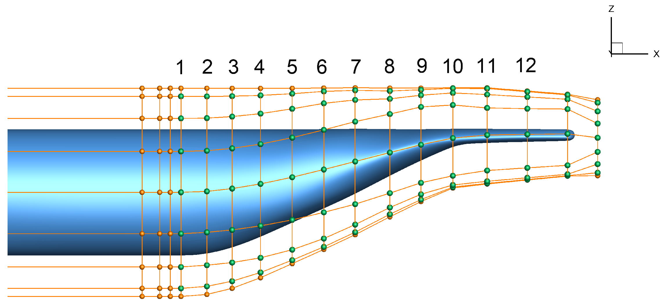
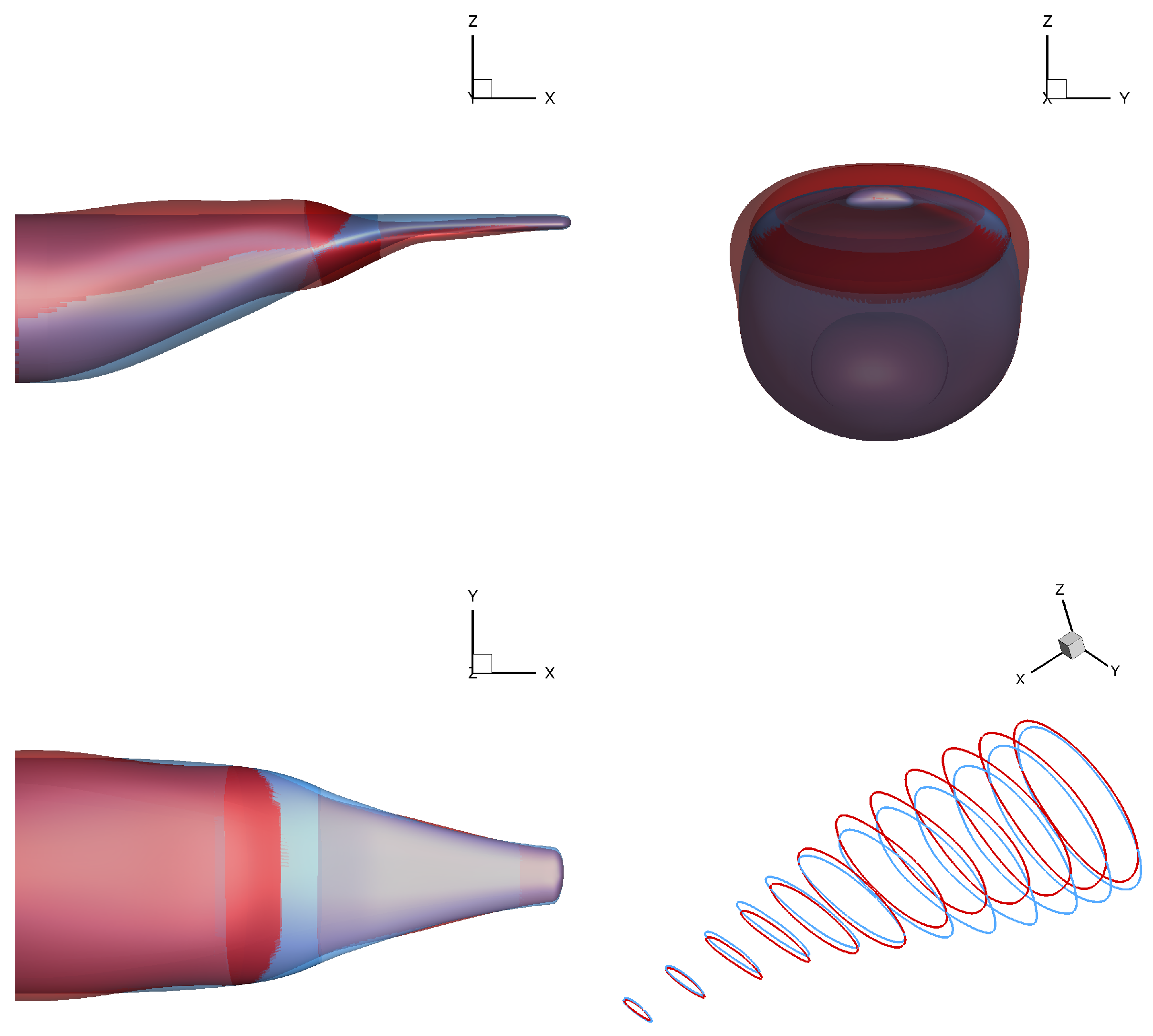
Eight cross-sectional positions along the axis of the fuselage are selected to show the evolution process of the afterbody vortex, as shown in Figure 17. Among them, the 8–12 section corresponds to the selection of Table 3 and Figure 11. The 13–15 section is the downstream detection section of the flow field. The positions are, respectively, x = 28.758 m, x = 29 m, and x = 30 m.
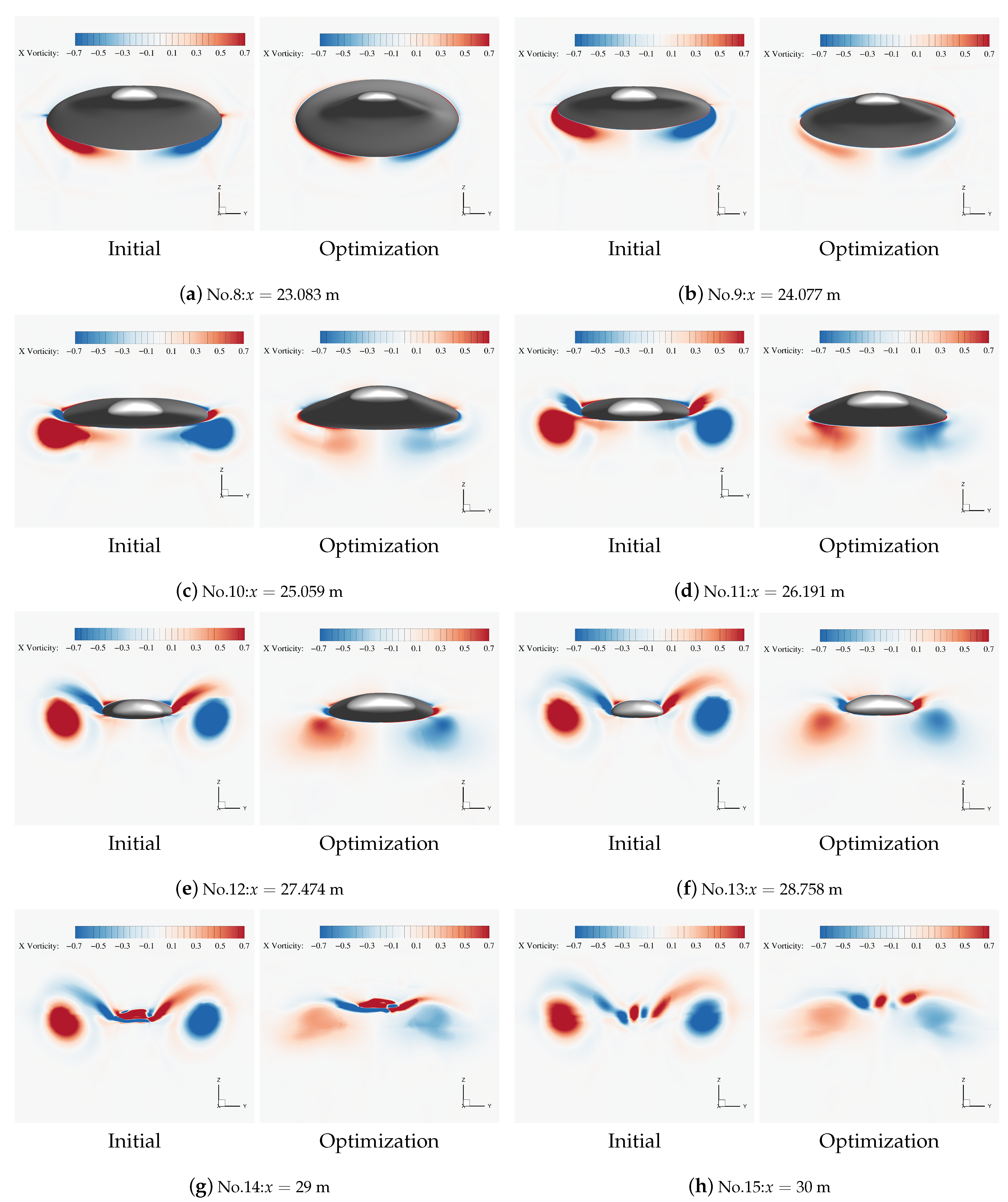
Figure 18 gives the x-vorticity contour at each cross-section. It contains the generated process and the downstream evolution of the afterbody vortex. The axial position ranges from x = 23.083 m to x = 30 m. The left side is the initial configuration, and the right side is the optimized configuration.
Using the boundary layer extraction method in Section 5, the boundary layer characteristics of a total of eight cross-sectional positions of the afterbody are extracted from 16.414 m to 23.084 m. The eight cross-sectional positions correspond to the selection in Table 3 and Figure 10, and they are all located at the position before the afterbody vortex detached point. 
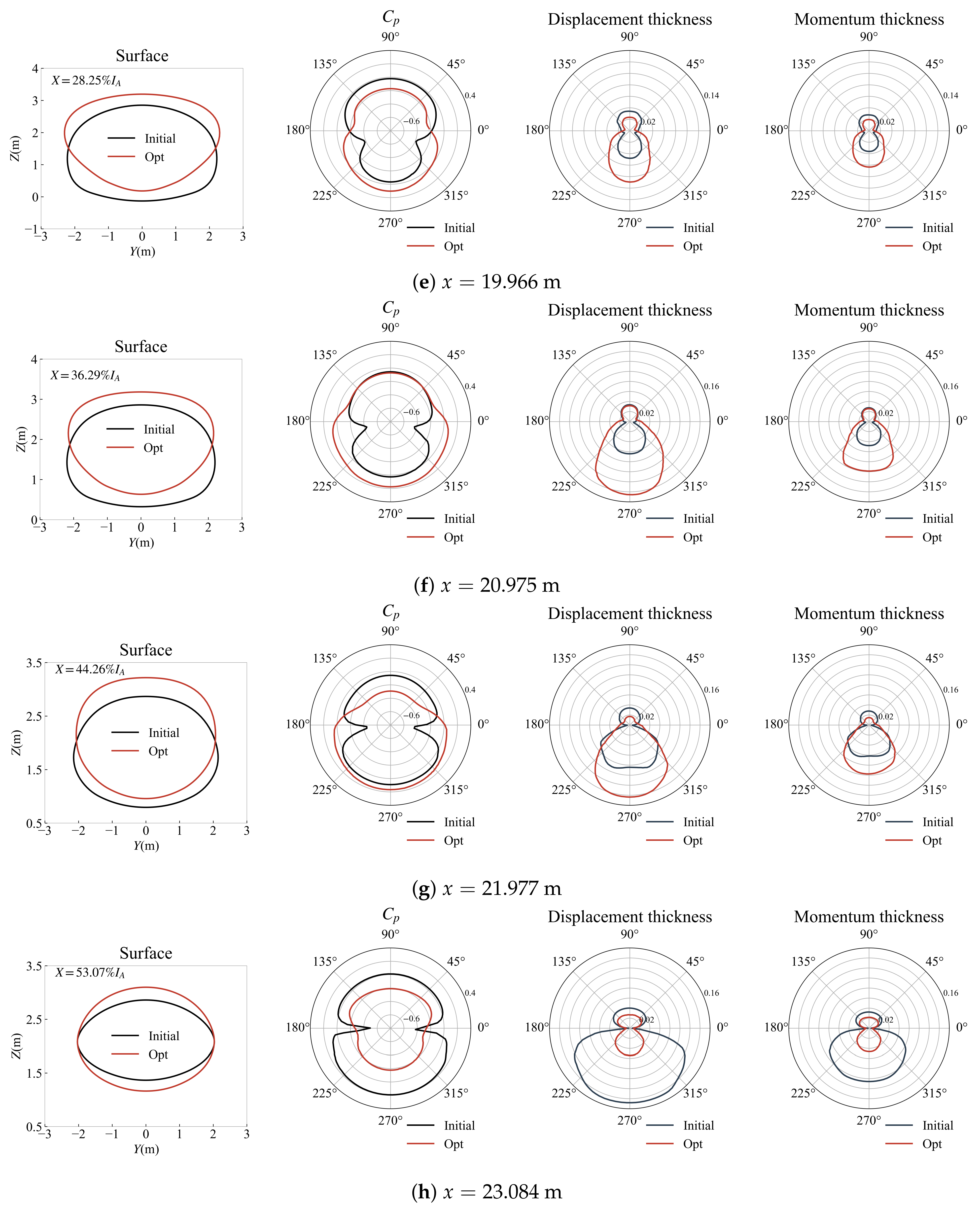
Figure 19 shows the changes in the shape of the cross-section before and after optimization at the 12 cross-sectional positions, the comparison of the circumferential pressure distribution, and the difference in the characteristics of the boundary layer, including the displacement thickness of the boundary layer and the momentum thickness of the boundary layer. Meanwhile, the velocity profile of the crossflow inside the boundary layer in the circumferential direction of each section is also displayed correspondingly in Figure 20. Each section has a total of eight stations from 0° to 315°. From the pressure distribution, after the position x = 18.047 m, near 0° and 180°, the initial configuration has a minimum circumferential pressure coefficient here, and there is a very intense circumferential pressure gradient, which also leads to the crossflow and the circumferential vorticity accumulation in this area, which can also be seen in Figure 18 at this location. The circumferential pressure distribution of the optimized configuration in each section is more uniform than the initial configuration, which slows down the circumferential transport process, thereby delaying the appearance of the detached point. Regarding the displacement thickness and momentum thickness of the boundary layer, the optimized configuration has a significant downward movement; that is, the boundary layer thickness of the upper fuselage is reduced while the thickness of the lower fuselage is greatly increased. The distribution pattern is similar in two characteristic parameters of the boundary layer. In the compressible flow, Equation (28) can be used to express the relationship between momentum thickness, displacement thickness, pressure distribution, and surface friction distribution. Equation (28) [46] shows that, as the pressure increases, the momentum thickness of the boundary layer should also increase. This also explains why the momentum thickness of the boundary layer in the lower fuselage of the optimized configuration continues to increase. However, it is worth noting that although the boundary layer thickness of the optimized configuration at the bottom of the fuselage is thicker than that of the initial configuration, the momentum thickness and displacement thickness of the boundary layer of the optimized configuration, around 0° and 180° (except for x = 20.975 m and x = 21.977 m), are smaller than the initial configuration, indicating that the optimized configuration has a more stable boundary layer in this location and has a stronger ability to resist the adverse pressure gradient and the trend of flow separation, thereby delaying the appearance of the detached point.
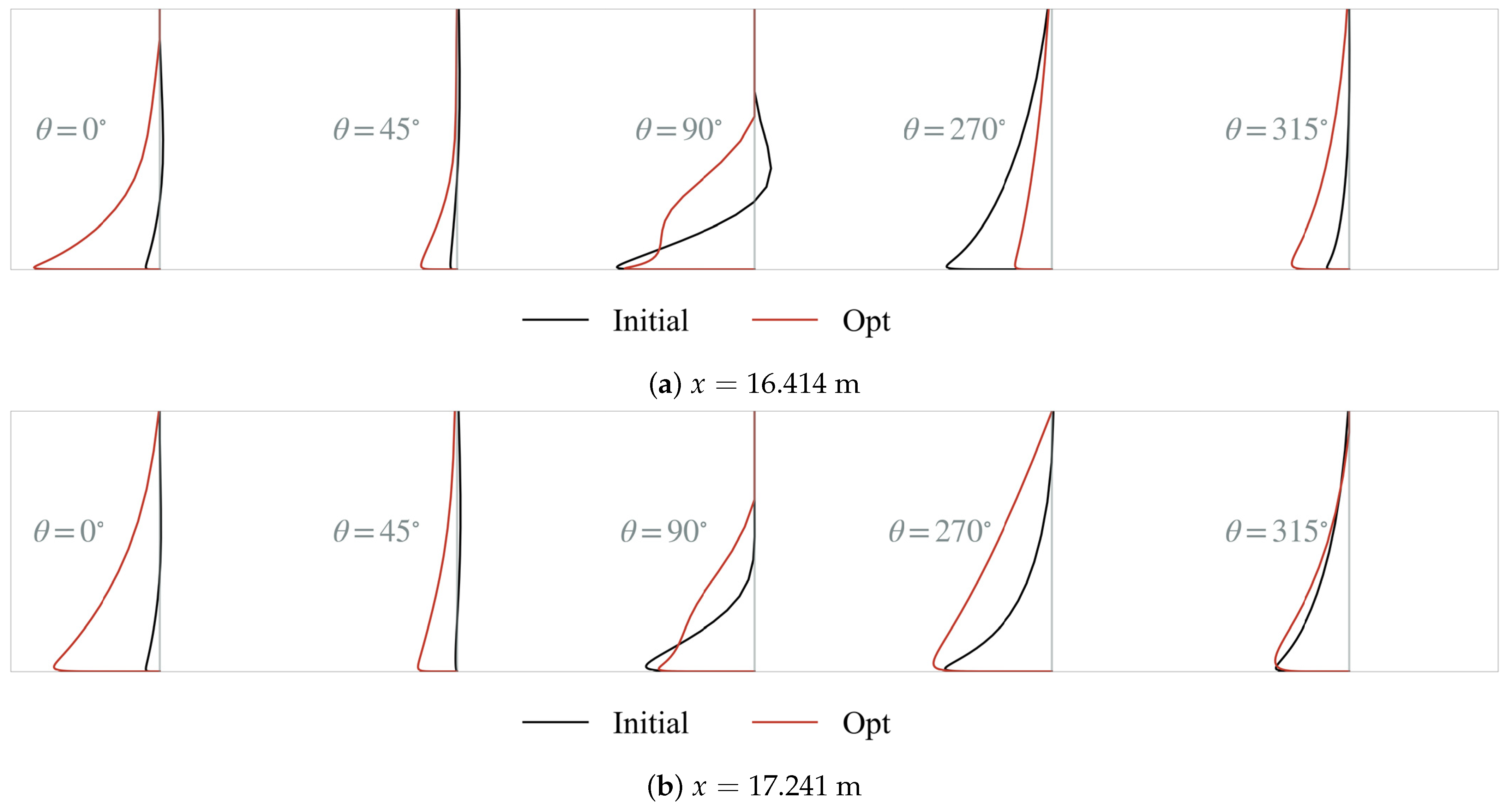
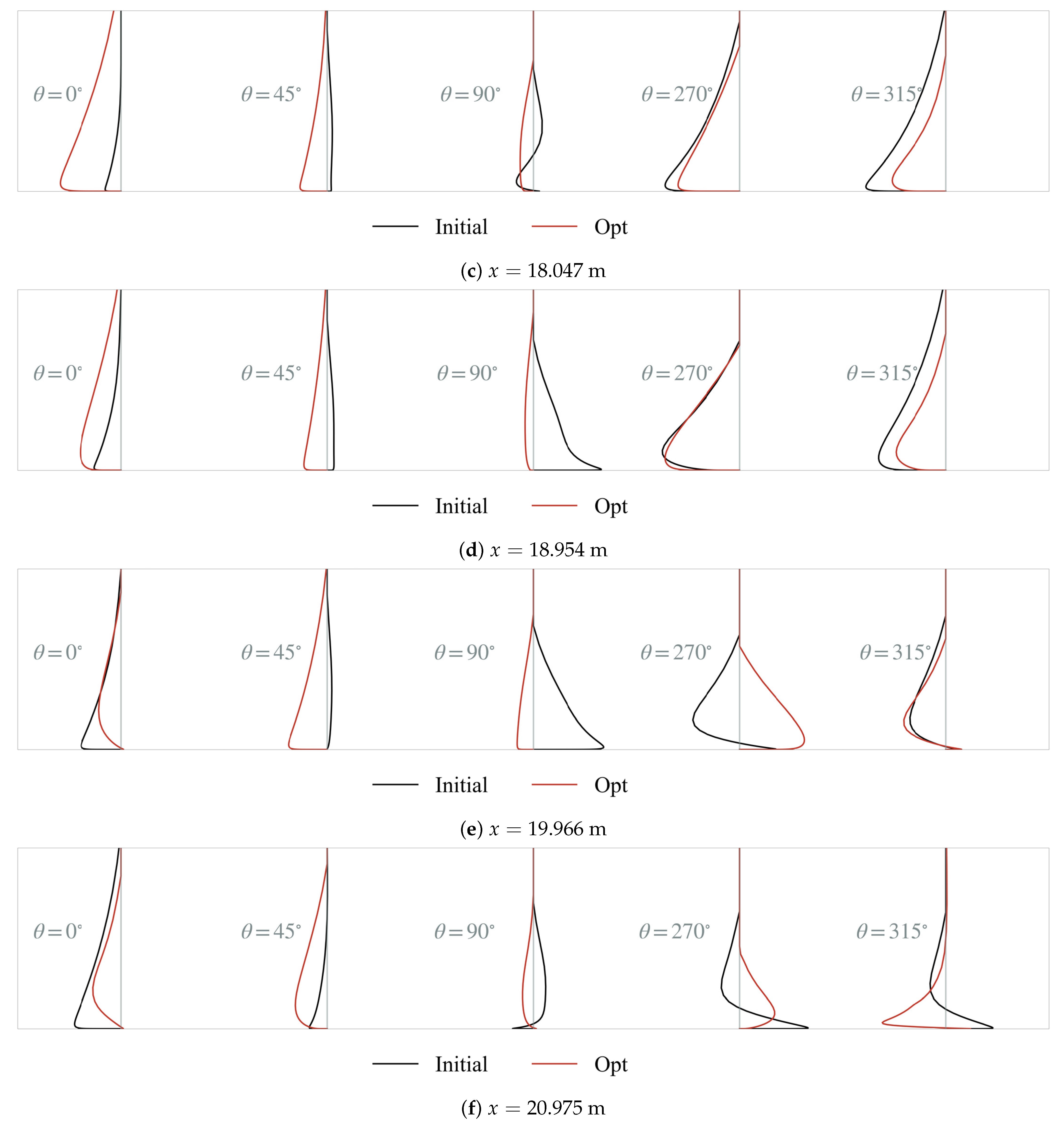
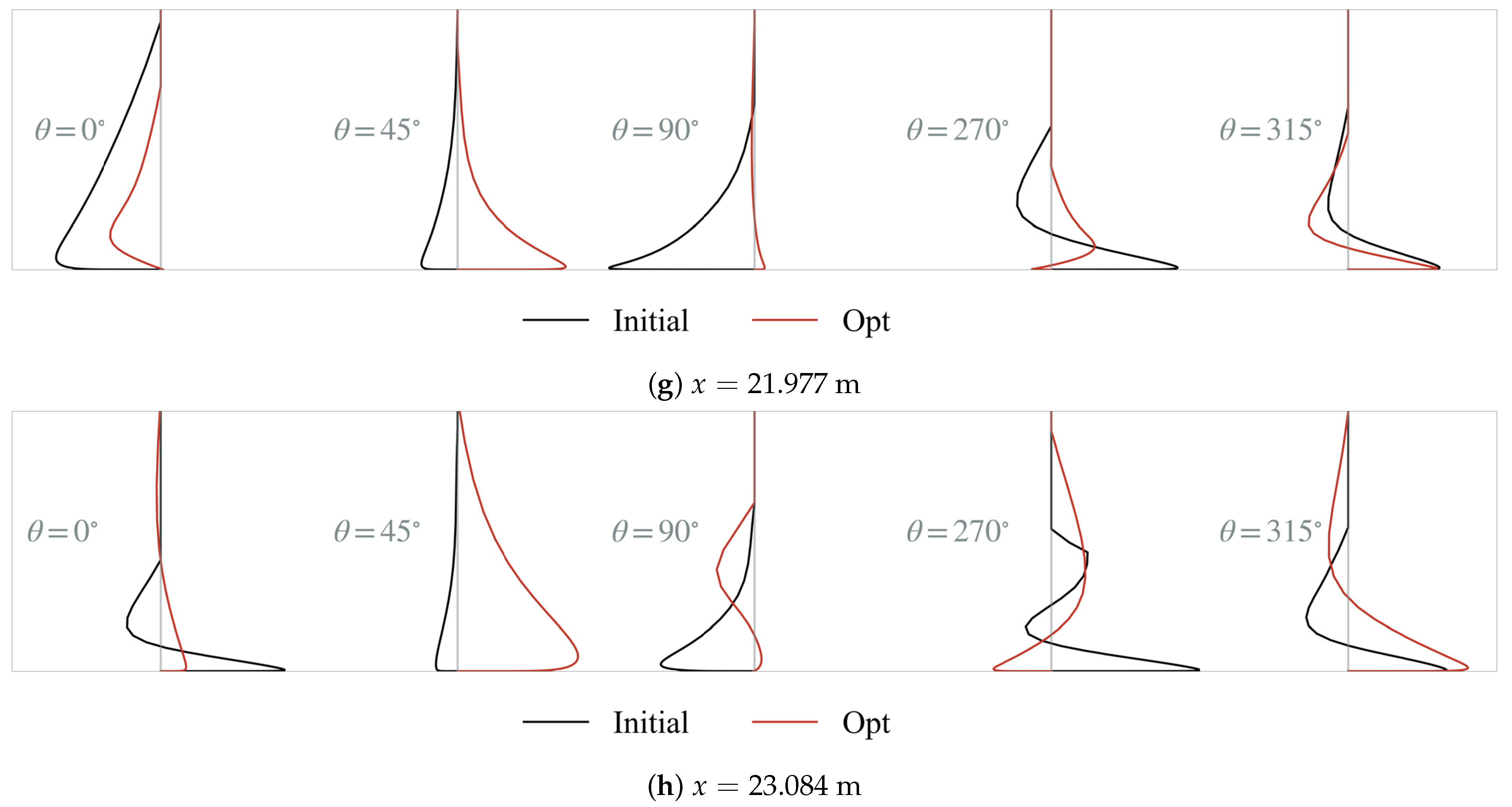
Paying attention to the crossflow velocity profile of the boundary layer in Figure 20, the crossflow intensity at the top (90°) and bottom (270°) of the fuselage in the optimized configuration has been significantly weakened, especially in the section near the detached point, as shown, e.g., in Figure 20f–h. At the 45° and 315° stations, the crossflow intensity does not change much before and after the optimization. The crossflow intensity of the 0° station after x = 19.966 m decreased greatly, and the closer it is to the detached point (ini: 24.5 m; opt: 25.5 m), the more the crossflow intensity weakens. Figure 16 shows that the positions of the saddle lines of the two configurations are close to the 0° station, and the decrease in the intensity of the crossflow at this position is also the main motivation for delaying the appearance of the saddle lines.
d d x ρ U 2 θ = δ * d p d x + τ ω
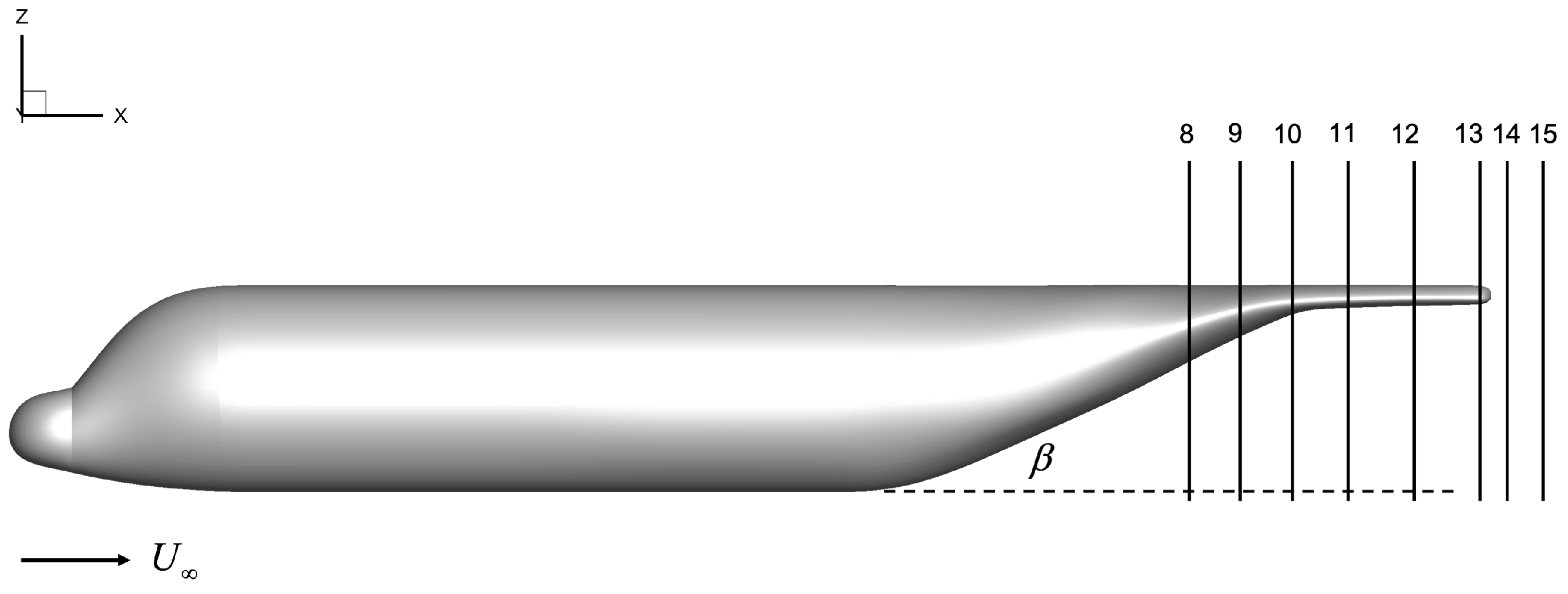
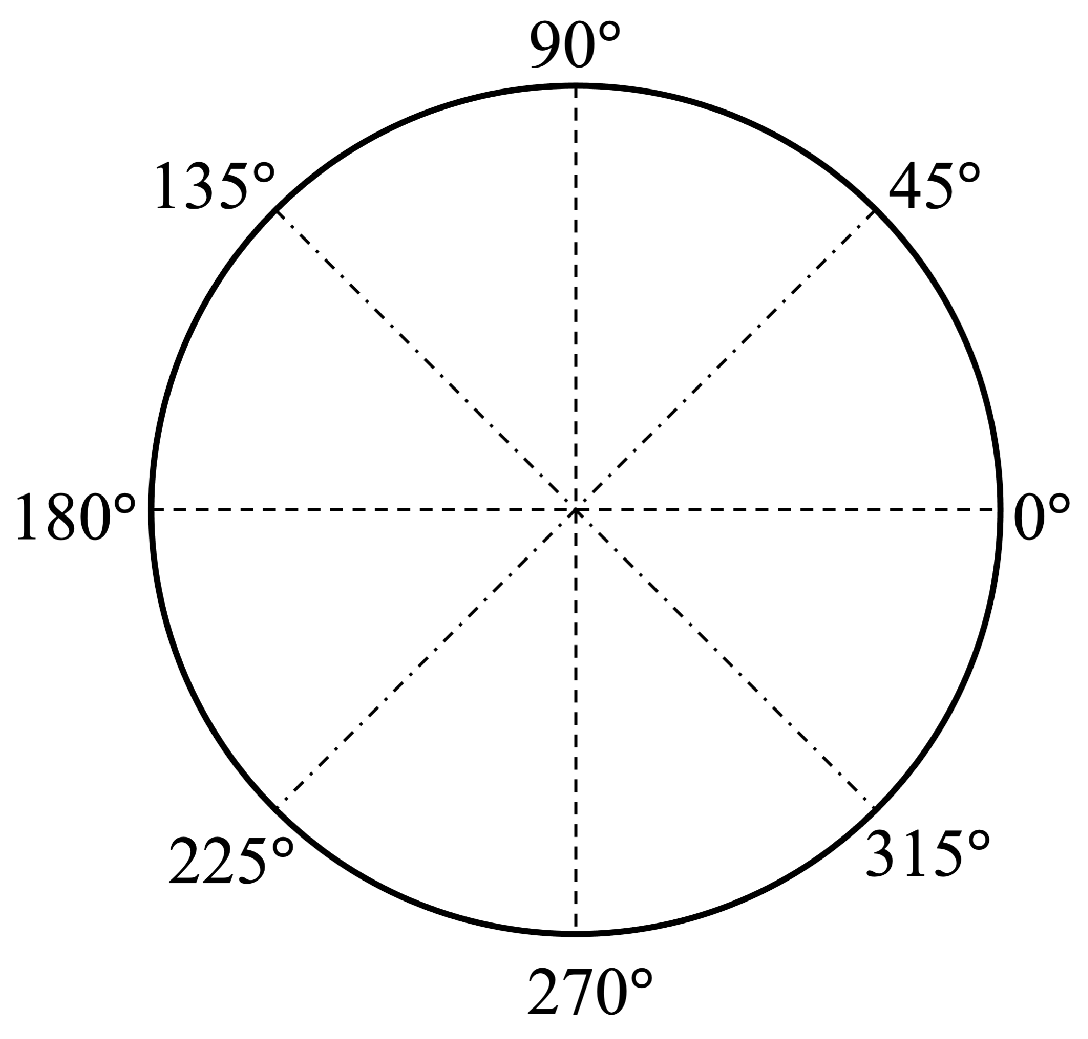
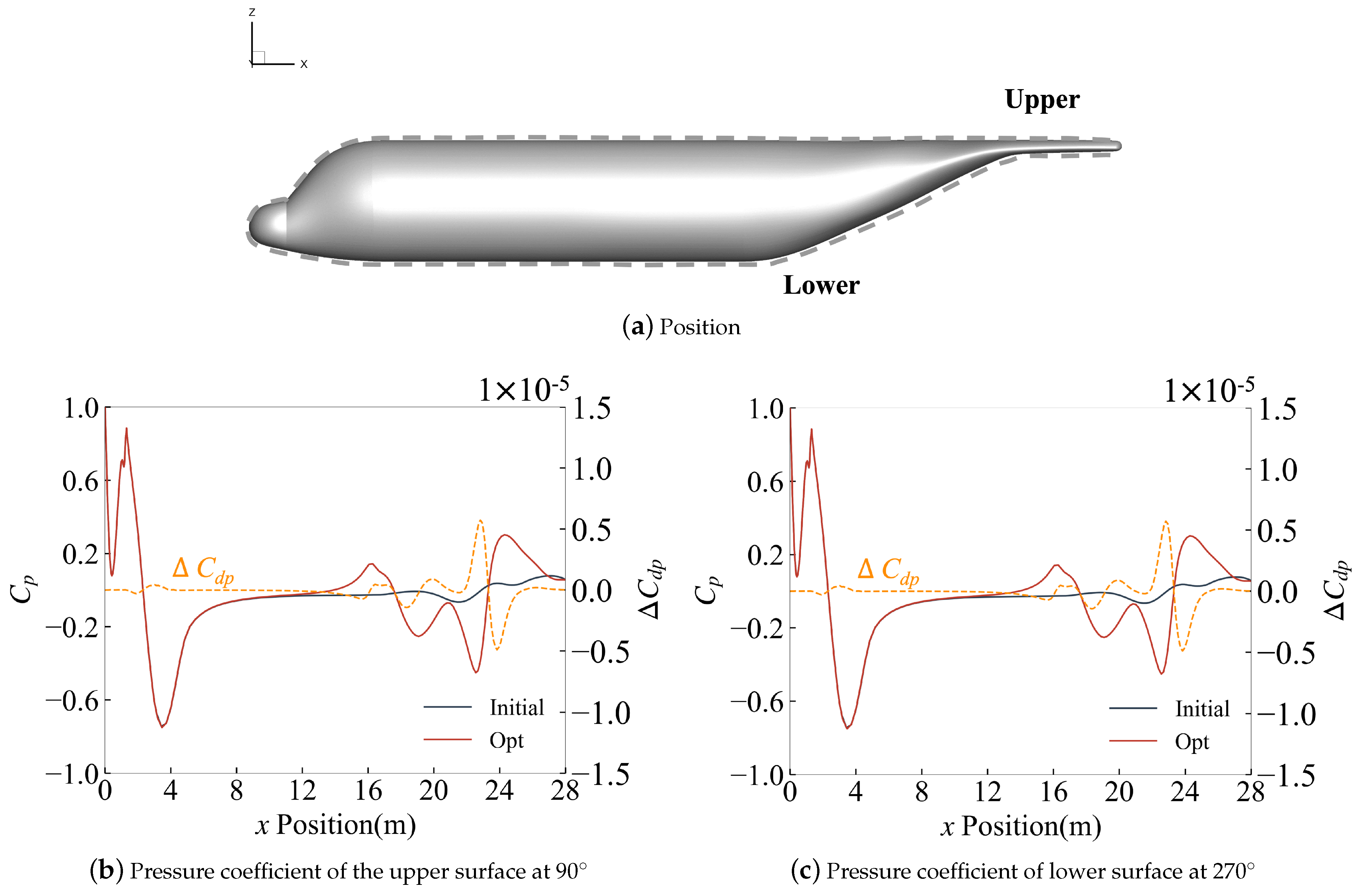
The typical angle of each slice of x coordinate is shown in Figure 21 where we mainly care about the top (90°) and bottom (270°) of the afterbody. The pressure coefficient of the surface along the top and bottom of the fuselage is extracted, as shown in Figure 22. The pressure coefficient at the bottom of the fuselage has changed significantly between 16 m and 25 m. The initial configuration has a long flow adverse pressure gradient in this interval. It is difficult for the boundary layer to continuously resist the adverse pressure gradient in this longer area. After optimization, the interval is decomposed into two shorter adverse pressure gradient regions and a favorable pressure gradient region, which effectively delays the separation trend of the boundary layer in the streamwise direction, thereby delaying the appearance of the detached point in Figure 16. The pressure distribution at the top of the optimized configuration fluctuates more than the initial configuration, which is due to the larger fluctuation of the upper surface due to the volume constraint during the optimization process. To compare the pressure drag more intuitively, the component of the pressure coefficient on the single grid element in the drag direction is defined as C d p , and the difference between the optimized configuration and the initial configuration is defined as Δ C d p = C d p o p t C d p i n i . Hence, Δ C d p < 0 results in the drag reduction effect. The orange dotted line in Figure 22 also depicts the distribution of the pressure drag from the nose to the tail of the fuselage at the top and bottom. The optimized configuration mainly has a significant reduction in the pressure drag at the bottom of the fuselage (270°), while the drag reduction effect at the top of the fuselage (90°) is not obvious. At the bottom of the fuselage (270°), although there are two areas where the pressure drag increases (16–17 m and 22–23 m) compared to the initial configuration, the pressure drag is decreasing overall because Δ C d p is negative in the wide range of 17–22 m. From the perspective of the corresponding pressure distribution, when the pressure coefficient of the optimized configuration is greater than that of the initial configuration, there is a drag reduction effect; conversely, when it is lower, the pressure drag is increased. Therefore, by reducing the pressure drag, the bottom of the fuselage is the dominant area, and the surface pressure coefficient should be increased. This can also be seen in Figure 19c,g; the pressure coefficient of the entire lower surface of the fuselage has increased significantly.
In general, both the initial configuration and the optimized configuration have evolved an apparent structure of the counter-rotating vortex wake downstream of the flow field. In the upstream of the formation of the afterbody vortex wake, the main flow phenomenon is the circumferential accumulation process of vorticity, which is motivated by the inverse pressure gradient brought by the bluff body in both the crossflow and the streamwise flow. The shear layer develops, and the vortex is transported down from either side of the upswept edge to the position where the condensed counter-rotating vortex pair is formed. During this period, the afterbody vortex remains attached to the solid wall.
The initial configuration at this stage is between x = 23.083 m and x = 24.078 m, while the optimized configuration is between x = 24.078 m and x = 25.059 m. It is obvious that the optimized configuration delays this trend of vorticity accumulation compared to the initial configuration.
As continuously obtaining vorticity from the boundary layer, the afterbody vortex ultimately sheds from the surface. A simultaneous displacement outboard can be seen as they appear to roll up back over the boundary layer. Small pockets of flow (also named the “corner vortex”) have diverse vorticity and circulation directions that emerge in the enclosed region between the vortices and boundary layer. This is due to secondary vortices generated by surface flow separation. It can be seen in Figure 16 that the detached point of the optimized configuration is closer to the tail of the aircraft than that of the initial configuration, which is also the reason for its lower vortex-induced drag.
When the afterbody vortex is completely separated from the wall, the shape of the vortex core gradually evolves from an irregular drop shape to a circle, for example, between x = 25.059 m and x = 26.191 m of the initial configuration. During the vortex develops downstream, the counter-rotating vortex triggers the upwash under its self-induced action, which displaces them and causes them to move vertically upwards; at the same time, the shape of the vortex core becomes elliptical, as shown in Figure 18f,h. The shape change of the vortex core can be verified in the flow field results of the initial configuration and the optimized configuration at the same time. 
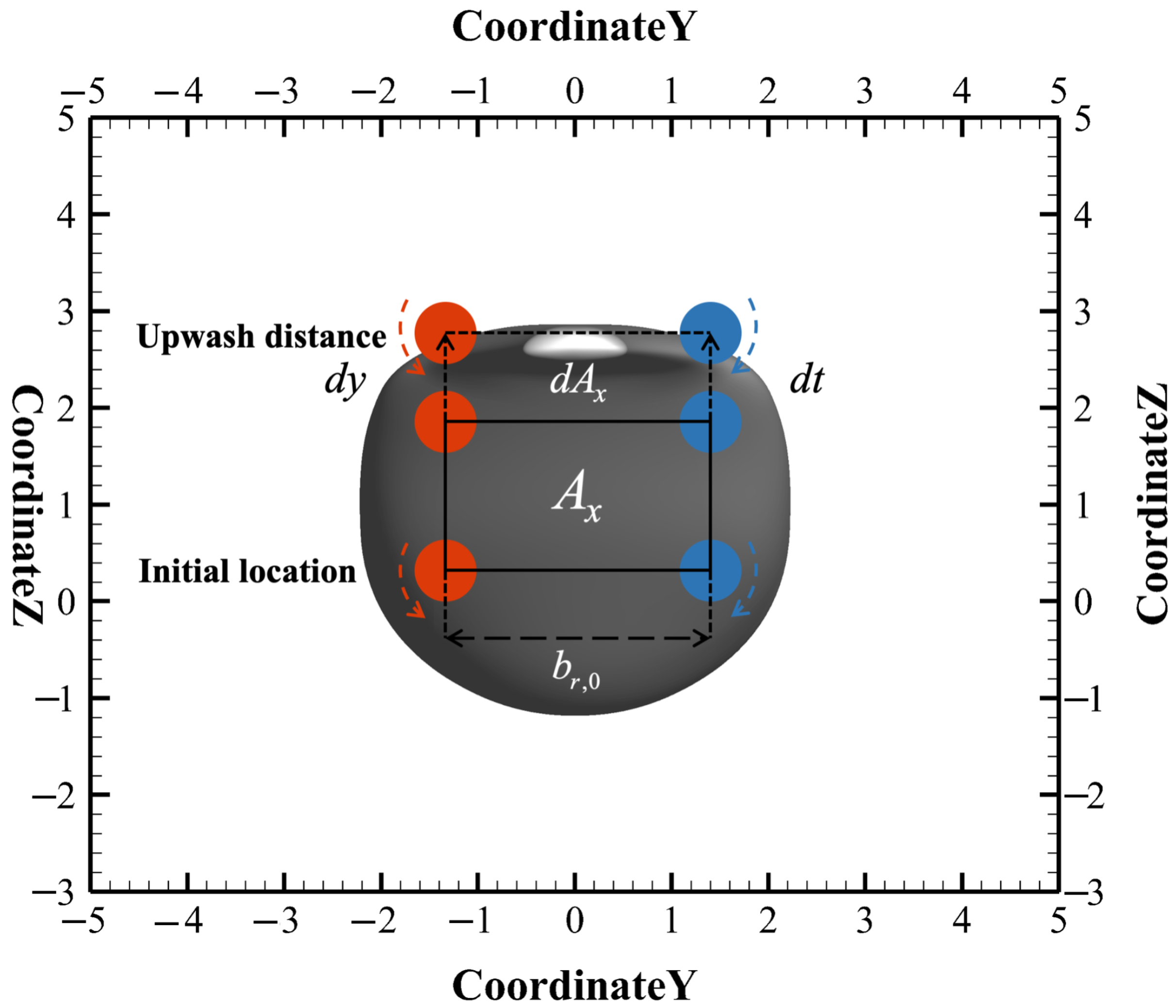
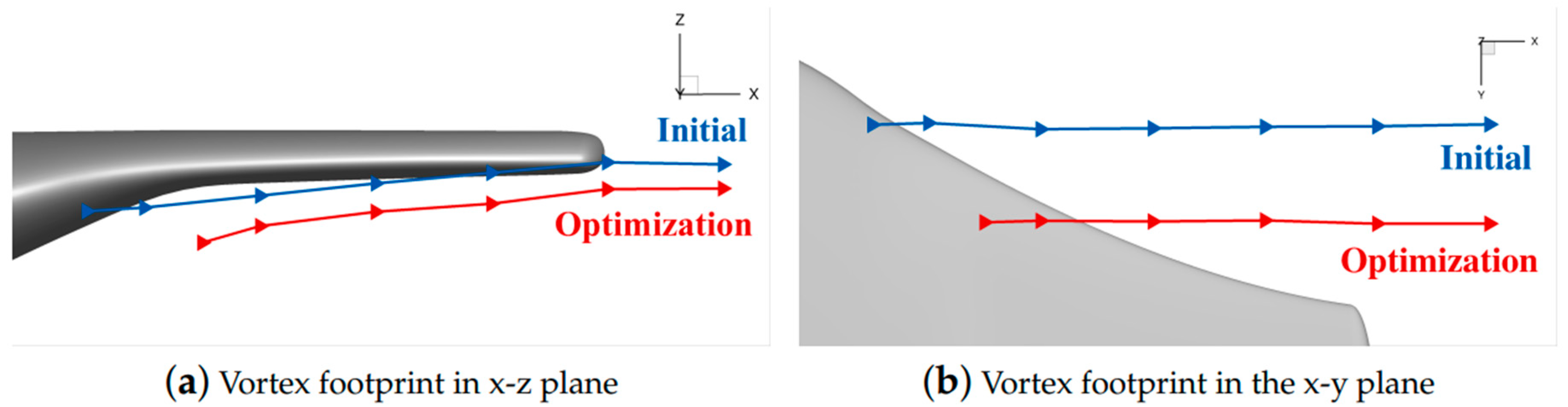
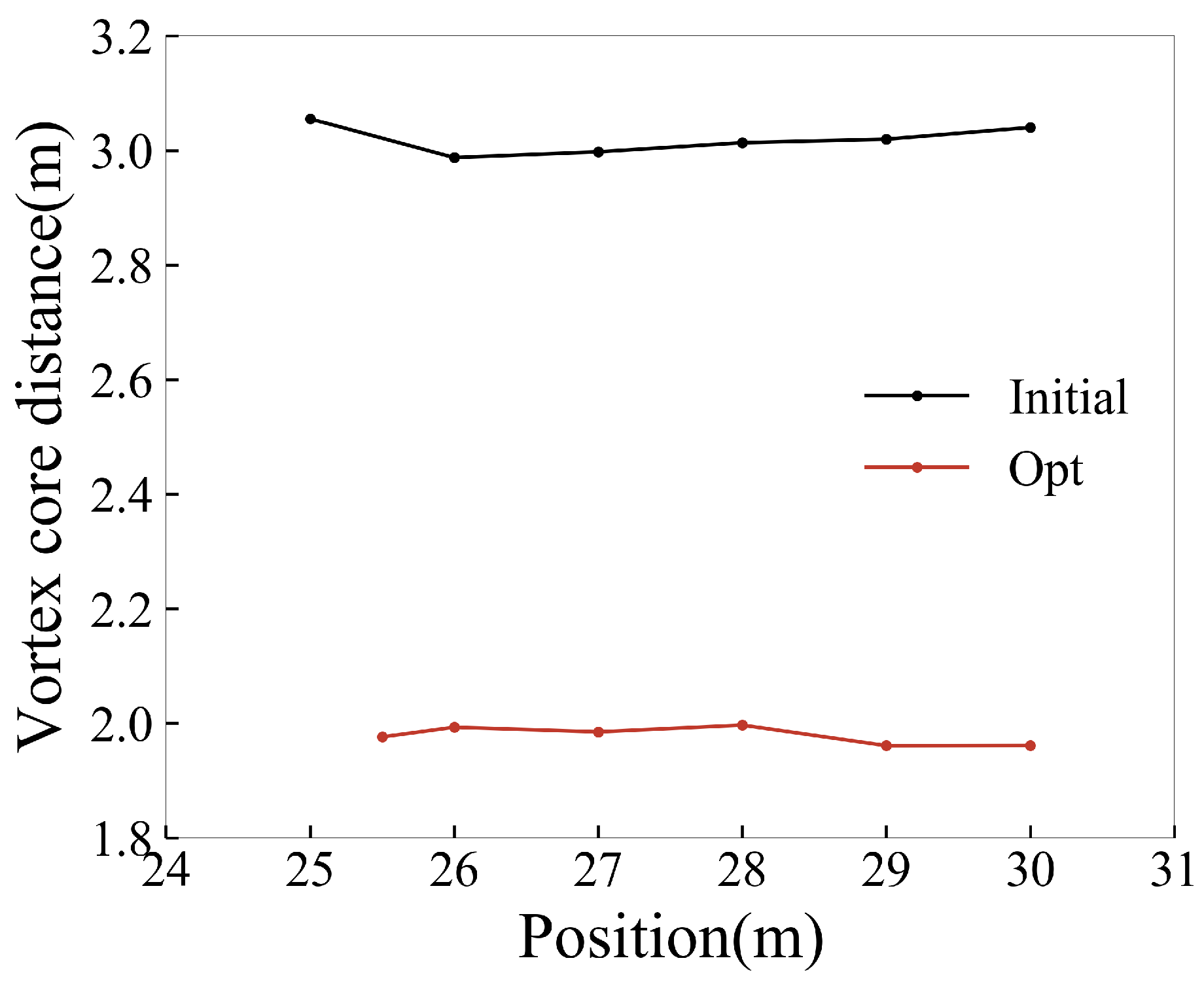
Figure 23 shows the displacement in the y-direction and the z-direction of the downstream vortex core for both the initial configuration and the optimized configuration. As shown in Figure 24, the distance between the left and right vortex remains invariable during the upwashing process of the counter-rotating vortex, which also shows that the vorticity loop model in Section 5.3 can characterize the evolution of the afterbody vortex system. Meanwhile, the distance between two vortex cores ( b r , 0 ) of the optimized configuration is much smaller than that of the initial configuration. 
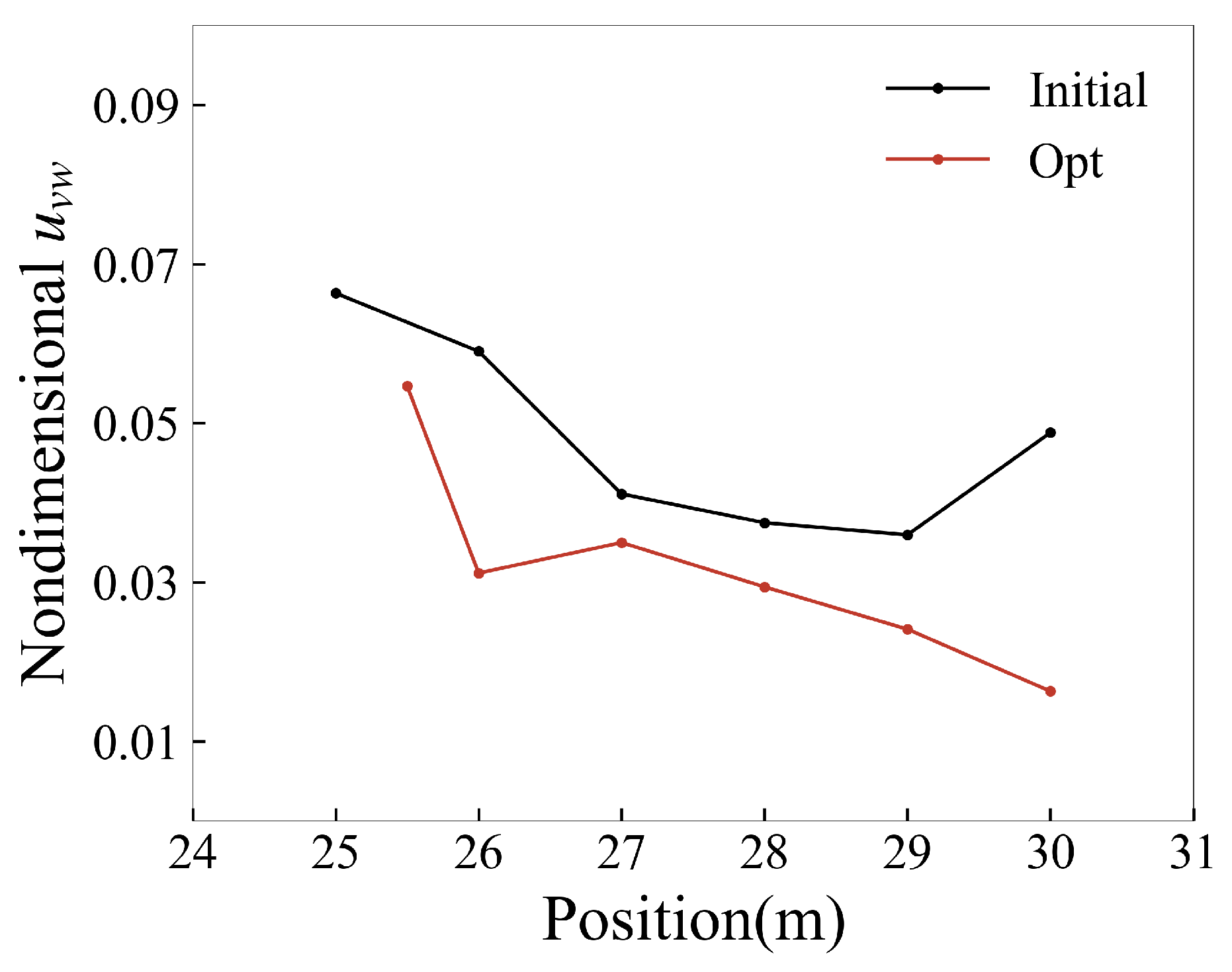
Figure 25 shows the change in the nondimensional upwash speed of the afterbody vortex core before and after the optimization along the streamwise direction, and the optimized configuration has a smaller upwash speed. According to Equation (26), the nondimensional vortex-induced drag coefficient of each section of the fuselage afterbody is obtained. The nondimensional vortex-induced drag coefficient of the optimized configuration is maintained within 4 counts, while the vortex-induced drag coefficient of the initial configuration is maintained within approximately 10–15 counts, as shown in Figure 26. By optimization, the vortex-induced drag coefficient is reduced by about 12 counts, which is close to the reduction in pressure drag shown in Figure 13.
To conclude, the optimization process of military transport aircraft is mainly to rationally change the flow direction and circumferential pressure distribution by the profile design so as to delay the accumulation of circumferential vorticity and the adverse pressure gradient of the flow direction and to weaken the strength of the crossflow, thereby delaying the location of the boundary layer vortex shedding. When the vortex finishes shedding, the distance between the vortex cores of the afterbody vortex decreases, and the upwashing speed decreases. To achieve the purpose of reducing vortex-induced drag and pressure drag, the vortex is farther away from the surface, reducing the impact on the surface, which is also concluded in [47].

8. Conclusions

The afterbody of the military transport aircraft was optimized by using the adjoint-based design optimization method. Based on the actual flight conditions, the design guidance of the afterbody parameters is given. The reasons for drag reduction after the optimization were analyzed.
The design optimization of the military transport aircraft has obvious drag reduction, mainly reducing the pressure drag, especially the vortex-induced drag caused by the detached vortex. Using the method of vortex dynamics and the theory of the vorticity loop model, the various processes of the afterbody vortex from generation and the shedding toward evolution were studied. From the point of view of design parameters, military transport aircraft should appropriately increase the flatness and reduce the change rate of the near-roundness in the axial direction of the fuselage. Based on the boundary layer extraction method, the upstream flow characteristics before the detached point were analyzed. The results show that the boundary layer momentum thickness and displacement thickness of the optimized configuration are significantly lower than those of the initial configuration. The characteristic thickness parameters of the boundary layer near the detached point are all significantly reduced. At the same time that the adverse pressure gradient of the optimized configuration in the circumferential direction is reduced, the crossflow intensity at most stations in the circumferential direction of the fuselage near the detached point is weakened, and the streamline convergence is decelerated, thereby delaying the appearance of saddle lines and vortex shedding. Due to the existence of the adverse pressure gradient when approaching the bluff body, the detached vortex of the afterbody is the result of the redistribution of the vorticity behind the upstream separation line of the bluff body. After the afterbody vortex completely sheds from the surface, the optimized configuration has a smaller vortex core interval, and the upwash speed of the vortex core center becomes smaller. Therefore, the vortex-induced drag is greatly reduced according to the vorticity loop model. As a result, the total drag decreased by about 23.2%.
The flow phenomenon we currently focus on will be advanced by considering the influence of wings and horizontal tails, which may be closer to reality. Some experimental studies and high-resolution CFD studies will be conducted to support the results.

Author Contributions

Conceptualization, H.R., Y.C., Y.S., T.Y. and H.L.; methodology, Y.C.; software, Y.C.; validation, H.R., Y.C., H.L. and T.Y.; formal analysis, H.R., Y.C., Y.S., T.Y. and H.L.; investigation, H.R., Y.C., Y.S., T.Y. and H.L.; resources, H.L., Y.S. and T.Y.; data curation, H.R., Y.C., Y.S., T.Y. and H.L.; writing—original draft preparation, H.R., Y.C., Y.S., T.Y. and H.L.; writing—review and editing, H.R., Y.C., Y.S., T.Y. and H.L.; visualization, H.R. and Y.C.; supervision, Y.S., T.Y. and H.L.; project administration, Y.S., T.Y. and H.L. All authors have read and agreed to the published version of the manuscript.

Funding

This research was funded by National Natural Science Foundation of China grant number 12002284.

Data Availability Statement

The data that support the findings of this study are available from the corresponding author upon reasonable request.

Conflicts of Interest

The authors declare that they have no known competing financial interests or personal relationships that could have appeared to influence the work reported in this paper.

Nomenclature

A Residual
A n The projection area of a vorticity loop in n direction.
b r , 0 The center distance of two counter-rotating wake vortex tubes
C D , v i Vortex-induded drag coefficient
C d Drag coefficient
C d p Pressure drag coefficient
C d v Viscous drag coefficient
C f Friction drag coefficient
C l Lift coefficient
C p Pressure coefficient
cConstraints
D Artificial viscosity
D ¯ v Time-average induced drag
d A , d B Diameter
FAerodynamic force
F s Safety ratio in GCI theory
F I , F V The inviscid flux term and the viscous flux term
h B The distance between the zero longitudinal down point of a certain normal section of the afterbody and the maximum width point
IObject function
L ¯ v Time-average induced lift
l A Length of afterbody
l F Length of fuselage
MMach number
pPressure
Q Conserved variables
qThe order of convergence
R e Reynolds number
R , R m a x Defined distance for near-roundness
R v Enclosed control volume
rThe position vector pointing to the fluid element from the origin
r g The grid refinement ratio
tTime
u v w The vortex wash speed in the vertical direction
UStreamwise velocity
VVolume
WFlatness
wThe maximum width of the section
x , y , z Cartesian coordinates
x s , x v Surface mesh and volume mesh
α Angle of attack
β Upswept angle
ζ Contraction ratio
η Nondimensional span location
λ Fineness
ϕ Near-roundness
δ e Boundary layer thickness
δ 1 , δ 2 Displacement and momentum boundary layer thickness
ω Vorticity
ρ Density
Γ v Induced circulation
Ω Vorticity tensor
τ w Shear stress on the wall

References

  1. Huang, Y.; Ghia, U.; Osswald, G.; Ghia, K. Analysis and numerical simulation of 3-D flow past axisymmetric afterbody using Navier-Stokes equations. In Proceedings of the 31st Aerospace Sciences Meeting, Reno, NV, USA, 11–14 January 1993; p. 682. [Google Scholar] [CrossRef]
  2. Epstein, R.J.; Carbonaro, M.C.; Caudron, F. Experimental investigation of the flowfield about an unswept afterbody. J. Aircr. 1994, 31, 1281–1290. [Google Scholar] [CrossRef]
  3. Hallstaff, T.; Brune, G. An investigation of civil transport aft body drag using a three-dimensional wake survey method. In Proceedings of the 13th Aerodynamic Testing Conference, San Diego, CA, USA, 5–7 March 1984; p. 614. [Google Scholar] [CrossRef]
  4. Zhang, B.; Wang, Y.Y.; Duan, Z.Y. Design method for large upswept afterbody of transport aircraft. Acta Aeronoutica Et Astronaut. Sin. 2010, 31, 1933–1939. [Google Scholar]
  5. Bury, Y.; Jardin, T.; Klöckner, A. Experimental investigation of the vortical activity in the close wake of a simplified military transport aircraft. Exp. Fluids 2013, 54, 1524. [Google Scholar] [CrossRef] [Green Version]
  6. Bai, J.; Sun, Z.; Dong, J.; Huang, J. Afterbody aerodynamic optimization design of transport airplane considering wing wake flow. Acta Aerodyn. Sin. 2015, 33, 134–141. [Google Scholar] [CrossRef]
  7. Morel, T. Effect of base slant on flow in the near wake of an axisymmetric cylinder. Aeronaut. Q. 1980, 31, 132–147. [Google Scholar] [CrossRef]
  8. Maull, D. The drag of slant-based bodies of revolution. Aeronaut. J. 1980, 84, 164–166. [Google Scholar] [CrossRef]
  9. Xia, X.; Bearman, P. An experimental investigation of the wake of an axisymmetric body with a slanted base. Aeronaut. Q. 1983, 34, 24–45. [Google Scholar] [CrossRef]
  10. Britcher, C.P.; Alcorn, C.W. Interference-free measurements of the subsonic aerodynamics of slanted-base ogive cylinders. AIAA J. 1991, 29, 520–525. [Google Scholar] [CrossRef]
  11. Bulathsinghala, D.; Jackson, R.; Wang, Z.; Gursul, I. Afterbody vortices of axisymmetric cylinders with a slanted base. Exp. Fluids 2017, 58, 60. [Google Scholar] [CrossRef] [Green Version]
  12. Wang, Y.; Qin, S.; Xiang, Y.; Liu, H. Interaction Mechanism of Vortex System Generated by Large Civil Aircraft Afterbody. J. Aeronaut. Astronaut. Aviat. 2017, 49, 65–74. [Google Scholar] [CrossRef]
  13. Wang, Y.; Qin, S.; Liu, H. Vortex drag generated by aircraft afterbody vorticity-loop system. In Proceedings of the AIAA Aerospace Sciences Meeting, Kissimmee, FL, USA, 8–12 January 2018; pp. 1–14. [Google Scholar] [CrossRef]
  14. Garmann, D.J.; Visbal, M.R. High-fidelity simulations of afterbody vortex flows. AIAA J. 2019, 57, 3980–3990. [Google Scholar] [CrossRef]
  15. Ranjan, R.; Robinet, J.C.; Gaitonde, D.V. Meandering of longitudinal wake vortices in slanted base afterbody flows. In Proceedings of the AIAA Scitech 2020 Forum, Orlando, FL, USA, 6–10 January 2020; p. 1532. [Google Scholar]
  16. Ranjan, R.; Robinet, J.C.; Gaitonde, D. Instability mechanisms in meandering streamwise vortex pairs of upswept afterbody wakes. Eur. J. Mech.-B/Fluids 2022, 96, 90–104. [Google Scholar] [CrossRef]
  17. Zigunov, F.; Sellappan, P.; Alvi, F. Reynolds number and slant angle effects on the flow over a slanted cylinder afterbody. J. Fluid Mech. 2020, 893. [Google Scholar] [CrossRef]
  18. Shi, L.; Yang, G.; Yao, S. Large eddy simulation of flow past a square cylinder with rounded leading corners: A comparison of 2D and 3D approaches. J. Mech. Sci. Technol. 2018, 32, 2671–2680. [Google Scholar] [CrossRef]
  19. Cravero, C.; Marogna, N.; Marsano, D. A Numerical Study of correlation between recirculation length and shedding frequency in vortex shedding phenomena. WSEAS Trans. Fluid Mech 2021, 16, 48–62. [Google Scholar] [CrossRef]
  20. Chen, X.; Zhong, S.; Ozer, O.; Weightman, A. Control of afterbody vortices from a slanted-base cylinder using sweeping jets. Phys. Fluids 2022, 34, 075115. [Google Scholar] [CrossRef]
  21. Zigunov, F.; Sellappan, P.; Alvi, F.S. Compressibility effects on the wake of a cylinder with a slanted afterbody. In Proceedings of the AIAA SCITECH 2022 Forum, San Diego, CA, USA, 3–7 January 2022; p. 0468. [Google Scholar]
  22. Huss, R.A.; Zigunov, F.; Sellappan, P.; Alvi, F.S. Mean Flow Topology of the Rounded Afterbody in Compressible Flow. In Proceedings of the AIAA SCITECH 2023 Forum, National Harbor, MD, USA, 23–27 January 2023; p. 1983. [Google Scholar]
  23. Johnson, W.; Trickey, C.; Forsythe, J.; Albertson, J.; Leigh, E. Experimental and computational investigation of the flow behind a C-130 with tailgate down. In Proceedings of the 40th AIAA Aerospace Sciences Meeting and Exhibit, Reno, NV, USA, 14–17 January 2022. [Google Scholar] [CrossRef]
  24. Bury, Y.; Morton, S.A.; Charles, R. Experimental investigation of the flow field in the close wake of a simplified C-130 shape a model approach of airflow influence on airdrop. In Proceedings of the Collection of Technical Papers—AIAA Applied Aerodynamics Conference, Honolulu, HI, USA, 18–21 August 2008; pp. 1–21. [Google Scholar] [CrossRef]
  25. Bergeron, K.; Cassez, J.F.; Bury, Y. Computational investigation of the upsweep flow field for a simplified C-130 shape. In Proceedings of the 47th AIAA Aerospace Sciences Meeting including the New Horizons Forum and Aerospace Exposition, Orlando, FL, USA, 5–8 January 2009. [Google Scholar] [CrossRef]
  26. Kolesar, C.; May, F. An afterbody drag prediction technique for military airlifters. In Proceedings of the Applied Aerodynamics Conference, Danvers, MA, USA, 13–15 July 1983; p. 1787. [Google Scholar] [CrossRef]
  27. Fanmei, K.; Jun, H.; Ya’nan, F.; Dong, Q. Effects of geometry parameters and flow parameters on drag coeficient of upswept afterbodies. J. Beijing Univ. Aeronaut. Astronaut. 2003, 29, 39–42. [Google Scholar] [CrossRef]
  28. Kong, F.; Hua, J.; Feng, Y.; Qiu, D.; Deng, X. Investigation of the flow mechanism on the afterbody with larger upswept angle. Acta Aerodyn. Sin. 2002, 20, 326–331. [Google Scholar] [CrossRef]
  29. Kong, F.M.; Hua, J.; Deng, X.Y.; Feng, Y.N.; Qiu, D. Analysis of the flows and the drag about upswept afterbodies. Acta Aerodyn. Sin. 2003, 21, 67–74. [Google Scholar] [CrossRef]
  30. Zhang, H.; Liu, C.; Qin, Y. The flow visualization of the different afterbody of the airliner. J. Hydrodyn. 2004, 19, 616–622. [Google Scholar] [CrossRef]
  31. Mao, X.; Zhang, B.; Wang, Y. Research on Parameters Influence of Fuselage Afterbody with LargeUpsweptAngleofTransportAircraf. Aeronaut. Comput. Tech. 2011, 41, 78–81. [Google Scholar] [CrossRef]
  32. Wang, Y.; Zhang, B.; Guo, Z.; Dong, Q. Aerodynamic optimization design for large upswept afterbody of transport aircraft based on FFD technology. Acta Aeronaut. Astronaut. Sin. 2013, 34, 1806–1814. [Google Scholar] [CrossRef]
  33. Yang, T.; Bai, J.; Wang, D.; Chen, S.; Xu, J.; Chen, Y. Aerodynamic Optimization Design for Afterbody of Tail-mounted Engine Layout Considering Interference of Engines. Acta Aeronaut. Et Astronaut. Sin. 2014, 35, 1836–1844. [Google Scholar] [CrossRef]
  34. Mader, C.A.; Kenway, G.K.; Yildirim, A.; Martins, J.R. ADflow: An open-source computational fluid dynamics solver for aerodynamic and multidisciplinary optimization. J. Aerosp. Inf. Syst. 2020, 17, 508–527. [Google Scholar] [CrossRef]
  35. Kenway, G.K.; Mader, C.A.; He, P.; Martins, J.R. Effective adjoint approaches for computational fluid dynamics. Prog. Aerosp. Sci. 2019, 110, 100542. [Google Scholar] [CrossRef]
  36. Roache, P.J.; Ghia, K.N.; White, F.M. Editorial policy statement on the control of numerical accuracy. J. Fluids Eng. 1986, 108, 2. [Google Scholar] [CrossRef] [Green Version]
  37. Roache, P.J. A method for uniform reporting of grid refinement studies. Asme-Publications-Fed 1993, 158, 109. [Google Scholar] [CrossRef]
  38. Spalart, P.; Allmaras, S. A one-equation turbulence model for aerodynamic flows. In Proceedings of the 30th Aerospace Sciences Meeting and Exhibit, Reno, NV, USA, 6–9 January 1992; p. 439. [Google Scholar] [CrossRef]
  39. Jameson, A.; Schmidt, W.; Turkel, E. Numerical solution of the Euler equations by finite volume methods using Runge Kutta time stepping schemes. In Proceedings of the 14th Fluid and Plasma Dynamics Conference, Palo Alto, CA, USA, 23–25 June 1981; p. 1259. [Google Scholar] [CrossRef] [Green Version]
  40. Klopfer, G.; Hung, C.; Van der Wijngaart, R.; Onufer, J. A diagonalized diagonal dominant alternating direction implicit (D3ADI) scheme and subiteration correction. In Proceedings of the 29th AIAA, Fluid Dynamics Conference, Albuquerque, NM, USA, 15–18 June 1998. [Google Scholar] [CrossRef]
  41. Biros, G.; Ghattas, O. Parallel Lagrange-Newton-Krylov-Schur Methods for PDE-Constrained Optimization. Part I: The Krylov–Schur Solver. SIAM J. Sci. Comput. 2005, 27, 687–713. [Google Scholar] [CrossRef] [Green Version]
  42. Yildirim, A.; Kenway, G.K.; Mader, C.A.; Martins, J.R. A Jacobian-free approximate Newton–Krylov startup strategy for RANS simulations. J. Comput. Phys. 2019, 397, 108741. [Google Scholar] [CrossRef]
  43. Hascoët, L.; Pascual, V. TAPENADE 2.1 User’s Guide. Ph.D. Thesis, INRIA, Paris, France, 2004. [Google Scholar]
  44. Jeong, J.; Hussain, F. On the identification of a vortex. J. Fluid Mech. 1995, 285, 69–94. [Google Scholar] [CrossRef]
  45. Wu, J.C. Theory for aerodynamic force and moment in viscous flows. AIAA J. 1981, 19, 432–441. [Google Scholar] [CrossRef]
  46. Green, J. Laminar flow control-back to the future? In Proceedings of the 38th Fluid Dynamics Conference and Exhibit, Seattle, WA, USA, 23–26 June 2008; p. 3738. [Google Scholar]
  47. Bulathsinghala, D.; Wang, Z.; Gursul, I. Drag reduction by manipulation of afterbody vortices. J. Aircr. 2018, 55, 2380–2391. [Google Scholar] [CrossRef]
Figure 1. The definition of afterbody design parameters.
Aerospace 10 00331 g001
Figure 2. The definitions of flatness and near-roundness.
Aerospace 10 00331 g002
Figure 3. Three views of the model.
Aerospace 10 00331 g003
Figure 4. Different mesh level.
Aerospace 10 00331 g004
Figure 5. Zoomed figure of the grid around the wall of afterbody and nose.
Aerospace 10 00331 g005
Figure 6. Common research model mesh.
Aerospace 10 00331 g006
Figure 7. The comparison of pressure distribution between ADflow solution and experiment ( η = 2 y / b is the span).
Aerospace 10 00331 g007
Figure 8. Design optimization framework.
Aerospace 10 00331 g008
Figure 9. The vorticity loop model.
Aerospace 10 00331 g009
Figure 10. The military transport aircraft FFD frame.
Aerospace 10 00331 g010
Figure 11. The military transport aircraft monitor section.
Aerospace 10 00331 g011
Figure 12. History of optimization for military transport aircraft.
Aerospace 10 00331 g012
Figure 13. The decomposition of drag for military transport aircraft.
Aerospace 10 00331 g013
Figure 14. Comparison of section parameters.
Aerospace 10 00331 g014
Figure 15. Surface comparison of military transport aircraft optimization (blue: initial; red: optimization).
Aerospace 10 00331 g015
Figure 16. Comparison of surface and volume flow field.
Aerospace 10 00331 g016
Figure 17. Slice position for monitoring the vorticity of military aircraft.
Aerospace 10 00331 g017
Figure 18. Comparison of x vorticity in eight cross-sectional positions of military aircraft.
Aerospace 10 00331 g018
Figure 19. Comparison of surface, pressure coefficient, displacement thickness, and momentum thickness in eight cross-sectional positions of military aircraft.
Aerospace 10 00331 g019aAerospace 10 00331 g019b
Figure 20. Comparison of crossflow velocity profile in eight cross-sectional positions of military aircraft.
Aerospace 10 00331 g020aAerospace 10 00331 g020bAerospace 10 00331 g020c
Figure 21. Typical angle of the fuselage.
Aerospace 10 00331 g021
Figure 22. Comparison of pressure coefficient on upper and lower surfaces.
Aerospace 10 00331 g022
Figure 23. Vortex footprint of the military aircraft.
Aerospace 10 00331 g023
Figure 24. Distance of the downstream vortex core.
Aerospace 10 00331 g024
Figure 25. Nondimensional upwashing speed.
Aerospace 10 00331 g025
Figure 26. Nondimensional vortex-induced drag.
Aerospace 10 00331 g026
Table 1. Parameters of the military transport aircraft model.
ParametersValue
Reference area ( m 2 )162.10
Fuselage length l F ( m ) 28.97
Maximum diameter d A ( m ) 4.035
Afterbody length l A ( m ) 12.568
Upswept angle β ( ) 24
Fineness λ 3.11
Contraction ratio ζ 0.095
Table 2. Mesh convergence study.
Mesh LevelMesh Size C d (Counts)GCI/%q
L21,396,66572.36/
L12,782,58570.6210.497
L0.54,936,34568.376.3842.6
Table 3. Monitored sections for military transport aircraft optimization.
(a) Section 1–6
ID123456
Position (m)16.41417.24118.04718.95419.96620.975
Percentage (%)06.5812.9920.2028.2536.29
Flatness0.90890.88580.81950.71400.59540.5021
Near-roundness0.90890.89450.84910.77010.66970.5751
(b) Section 7–12
ID789101112
Position (m)21.97723.08424.07825.09626.19127.474
Percentage (%)44.2653.0760.9869.0877.7988.00
Flatness0.43450.35070.28030.17220.16020.2132
Near-roundness0.48220.36710.28030.20810.21590.2791
Table 4. Optimization results for military transport aircraft.
ConfigurationDrag Coefficient ( C D )Lift Coefficient ( C L )
Initial0.00707−0.0144
Optimized0.00543−0.0049
Δ /%16.4 counts/−23.2%65.97%
Disclaimer/Publisher’s Note: The statements, opinions and data contained in all publications are solely those of the individual author(s) and contributor(s) and not of MDPI and/or the editor(s). MDPI and/or the editor(s) disclaim responsibility for any injury to people or property resulting from any ideas, methods, instructions or products referred to in the content.

