
Time-Series-Data Interpolation Applied to Boundary-Layer Profiles Measured on Different Flights

Aviation Technology Directorate, Japan Aerospace Exploration Agency, Chofu, Tokyo 182-8522, Japan
*
Author to whom correspondence should be addressed.
Aerospace 2023, 10(4), 322; https://doi.org/10.3390/aerospace10040322
Submission received: 8 February 2023
/
Revised: 7 March 2023
/
Accepted: 16 March 2023
/
Published: 23 March 2023
(This article belongs to the Special Issue Flow Control and Drag Reduction)
Abstract
:Turbulent boundary-layer profiles on an aircraft surface were measured during flight by pitot rakes in an experiment at subsonic speeds. Because separate flights have different flight sequences in terms of time, it is not easy to compare boundary-layer profiles measured on different flights with the corresponding premised conditions directly. Using one flight as a reference, this paper proposes a method to find the closest flight condition for each time instance from data from other flights by calculating a residual norm in combinations of flight variables. The results show that the proposed method successfully finds the best matches of the time instances from the second flight with those of the first flight. In addition, applying the interpolation method using response surface methodology further improves the accuracy of evaluation in the flight range of Mach 0.4 to Mach 0.8. The total uncertainty level of the proposed interpolation method was found to be 5.7%. Although this level of uncertainty is expected to be reduced, the effectiveness of the proposed interpolation method was presented in conjunction with an evaluation of its applicability to determine the riblet effect in reducing skin-friction drag qualitatively.
1. Introduction
As the volume of trans- and intercontinental air travel increases, the need for more economical aircraft is growing, and it must be met while minimizing environmental disturbances, such as carbon-dioxide emissions. In addition to global-warming considerations, it is vital to improve aerodynamic efficiency and to reduce aerodynamic drag in these environmentally-friendly aircraft. Since skin friction drag constitutes more than half of total aircraft drag [1], reducing it is key to increasing aerodynamic performance and reducing fuel consumption. Skin friction drag is strongly related to boundary-layer profiles, which are important to characterizing its mechanism, so it is vital to control the boundary-layer profiles as well as designing aircraft with high performance while minimizing drag and noise [2].
There are a number of techniques that can control a boundary layer, such as suction [3,4], blowing [5], synthetic jets [6], vortex generators [7,8], leading-edge tubercles [9], and riblets [1,10,11,12,13,14,15,16,17,18,19,20,21,22,23,24,25,26,27]. Among those techniques, riblets are a passive means of turbulent flow control to reduce skin-friction drag and were first used at the NASA Langley Research Center in the 1970s [12,16]. They were inspired by the skin structure of sharks, which allow them to swim long distances at high speeds. A riblet is a groove in the skin of an object aligned in the flow direction. It induces a streamwise vortex structure to control the turbulent structure responsible for surface drag, so that turbulent skin friction drag is reduced.
The Japan Aerospace Exploration Agency (JAXA) has been working on environmentally friendly aircraft research with the aim of reducing drag, including skin friction drag [28,29,30]. As part of this research, a project named Flight Investigation of skiN-friction reducing Eco-coating (FINE) [23,28], which aims to investigate the effectiveness of JAXA-designed riblets on reducing skin friction drag, flight experiments using JAXA’s flight-test bed [31] were conducted. The boundary-layer profiles on the aircraft surface were measured using pitot rakes, which were attached to the outside of the aircraft fuselage. A major concern arising from the boundary-layer measurements taken over several flights is that the velocity profiles of the boundary layer can differ between flights. This can occur because of slight differences in flight attitudes and conditions arising from remaining fuel weight and atmospheric conditions, although identical flight conditions were assumed between the flights in the study. Because the pitot-rake measurement is sensitive to the environment, the boundary-layer profiles differ in terms of their shapes and absolute velocities. Therefore, the boundary-layer profile can change with the flight condition, as well as depending on whether drag-reducing devices, such as riblets, are used. Therefore, there is some difficulty in properly evaluating the effectiveness of riblets, since the magnitude of any reduction would be on the order of several percent. In most test scenarios, boundary-layer profiles with and without riblets are obtained over several flights. Therefore, it is vital to eliminate or minimize the influence of the flight conditions on boundary-layer profiles.
To this end, a previous study [32] introduced an approach that uses an interpolation method based on the response surface methodology (RSM). The RSM has been applied to aerodynamic optimization studies and data fitting to reduce errors in the data acquired in flight conditions [33,34,35,36,37]. Rosenbaum et al. [33] and Sevant et al. [34] applied the RSM to design the wing geometry of aircraft. Zhang et al. [35] applied the RSM to a coupling problem between the shape optimization and flow control in order to improve the performance of wings and blades. Papila et al. [36] applied the RSM to reduce both noise and modeling errors in the design of a high-speed civil-transport wing structure, and successfully demonstrated a reduction in the errors inherent in the modeling and optimization of the wing geometry and structure [36]. The RSM can also be used to estimate a geometry of interest that is being optimized [37]. Walsh et al. [38] used a multiple regression analysis to fit data obtained under flight conditions to estimate the data trend by reducing the measurement uncertainty [38]. This method is similar to the data-interpolation method based on the RSM. Thus, the response surface methodology has been widely applied to aerodynamic optimization studies and data fitting to obtain the data trend by reducing uncertainty. The proposed method using the RSM [32] enables the interpolation of the boundary-layer velocity profile obtained in a flight to that in another flight under the same premised flight conditions by removing the individual flights’ conditional influence, such as the angle of attack or slight discrepancies in flight conditions due to the atmosphere.
Given premised time-averaged target conditions, this method has successfully interpolated the boundary-layer velocity profile by removing the influence of individual flights with an error level of 4.1% for a flight Mach number range of 0.5–0.78 [32]. Thus, the boundary-layer-velocity profiles measured during different flights assuming the same flight conditions can be compared equivalently. Note that a previous study [32] applied the interpolation method for a riblet study at a premised nondimensional riblet width only to target flight conditions in which the aircraft attitude was in a semi-cruise condition. This testing scenario limited the available data to only five cases per flight [32]. The limited datasets made it difficult to evaluate some of the effects of the devices, such as drag reduction.
A new approach was proposed to expand the number of available datasets in this study. This approach uses all the time-series data obtained during a flight, including the data from just after take-off until just before landing. In the previous method [32], the reference case and the compared case both used 60-s-averaged measurements for a target condition made by a nondimensional riblet width. The present study aims to determine the closest match between the conditions of the compared flight and the reference conditions. This will enable the search for the most closely matched conditions between two different flights at each time instance during all the flight phases.
In this study, based on the measured boundary-layer profile (i.e., the U-velocity profile) on the aircraft-fuselage surface using pitot rakes in flight conditions, the proposed method was evaluated with regard to its accuracy in time-series datasets. Next, its applicability to the effect of riblets in reducing the skin friction drag in a qualitative manner was evaluated, and is reported herein.
2. Flight-Test Bed, Measurement System and Equipment, and Test Conditions
2.1. Flight-Test Bed and Measurement System Onboard
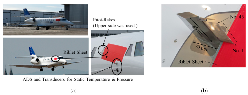
Figure 1a shows the flight-test bed and pitot rakes with static pressure and temperature ports implemented on the airframe surface. Since this study is the continuation of the work in a previous study [32], the same instrumentation was used for measuring the boundary-layer-profile data. This study emphasizes the effect of the post-processing method on the boundary-layer-profile interpolation. The air-data system (ADS) was mounted near the front of the aircraft, as shown in Figure 1a, for sensing air data, such as the Mach number, pressure, temperature, angle of attack, and angle of sideslip. The accuracy of the sensed air data was, for example, 0.4% for a measured Mach number. Two pitot rakes were located behind the riblet sheet, which had a cord length of 1306 mm, an effective span length of 574 mm, and a thickness of 100 μm.
The pitot-rake measurement was employed to measure the boundary-layer profiles in the aircraft fuselage. The velocity profile in the boundary layer can be determined directly by using the pitot-rake measurement, which is a reliable method using highly accurate pressure transducers [39,40]. The measured velocity profile is a time-averaged value as the pitot-rake measurement involves a pneumatic probe system. The pitot rake was made of a rigid stainless-steel structure and was mounted on a metal surface that replaced the original window, as shown in Figure 1a.
Figure 1b shows a detail of the pitot rake, which consists of 45 single-hole probes for measuring pitot pressures to identify the boundary-layer profile in the aircraft fuselage. The minimum probe diameter employed in this study was 0.5 mm. The pitot rakes were aligned assuming that they were located on the streamline along the fuselage, as estimated by the numerical simulation [23]. Note that the actual streamline can depend on the flight conditions and, hence, the location of the pitot rake may not be aligned with the flow under off-design flight conditions. However, it should be noted that the pitot rake was assumed to measure the streamwise velocity of the flow, accounting for past studies [41] that showed that the measurement accuracy was ensured up to an angle of attack of 20° at a Mach number of 0.64 [41]. Furthermore, a wind-tunnel-calibration experiment, which was conducted prior to the flight experiment [29], showed that the uncertainty in measuring the pitot pressure for the designed pitot rake can be negligible in the range of an angle of attack of less than ±5° [29]. Thus, the pitot rake was considered to measure the streamwise velocity profile of the flow in the aircraft fuselage when the flight conditions were at a steady target rate. The on-design condition data are used for a comparison with the time-series data analysis proposed in this study. The cross-section of the aft part of the pitot rake is a rhombus that avoids the generation of extra lift and vibration, which can be introduced by an unstable flow separation. The accuracy of the pitot-rake measurement was approximately 3.5%, which was calculated as a maximum error obtained as a ratio of 1σ over a velocity averaged over 1 min under on-design conditions for all the probes.
The measurement system onboard the aircraft consisted of a data recorder and transducers for measuring the pitot pressure, static pressure, and static temperature. Each measured signal was recorded by a laptop computer at a sampling frequency of 10 Hz.
2.2. Paint-Based Riblet
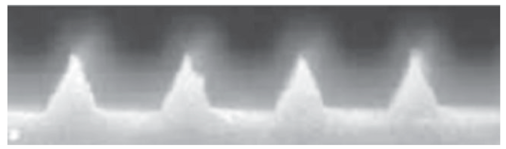
The riblet surface was fabricated from an aviation-paint-based material and was designed by JAXA’s FINE project. The paint-based riblet had grooves aligned in the streamwise direction, as shown in Figure 2, which shows a photograph of one cross-sectional plane of the riblet. The width (s) or inner spacing between two neighboring grooves was 100 μm [30].
Six flight experiments were conducted in 2017 and five in 2018 during the flight-test campaign of the FINE project. For the experiment campaign in 2017, the riblet width was 170 μm [32,42], and that for 2018 was 100 μm. This paper focuses on using the results of the 2018 experiments. In addition, this study presents a representative case for each wall condition of each flight: reference (first flight with a smooth wall) and compared (second flight with a wall with a riblet) cases.
2.3. Test Conditions
The primary parameter used in this study is expressed as Equation (1), which is a nondimensional riblet width and, essentially, a Reynolds number based on the riblet width and friction velocity. This parameter was used to determine the flight Mach number and altitude conditions, details of which are described below. Equation (2) calculates the local skin-friction coefficient based on the momentum thickness of the local boundary layer.
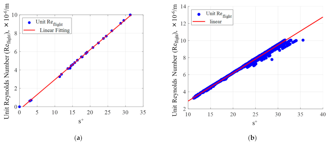
Equation (1) is also used for evaluating the effect of the riblet on reducing skin friction drag. Note that the effectiveness depends on the turbulent eddy size in the boundary layer and the riblet valley’s width; therefore, it is strongly related to the Reynolds number, which is expressed as the unit Reynolds number based on the flight Mach number and static temperature, which also corresponds to the flight altitude. The Reynolds number is expressed as Equation (3). The relationship between s+ (Equation (1)) and (or Reflight) (Equation (3)) is presented in Figure 3a for assumed on-design conditions at semi-cruise conditions described in Section 2.1 and in Figure 3b for all time-series data, including off-design conditions from take-off to landing. Note that Figure 3a corresponds to the conditions and analysis presented in a previous study [32] and Figure 3b shows extended data for all time-series data obtained during one flight.
As shown in Figure 3a, s+ has a linear relationship with with R2 value of 0.99 for these variables. Figure 3b also shows strong linearity between the two variables, although slight discrepancies can be seen. This kind of discrepancy and outliers from the linear fit correspond to near-take-off and -landing conditions. Therefore, while the flight condition becomes stable regardless of whether it is in ascent/descent or cruising, these two variables are linearly related. For this reason, s+ is used to define flight conditions, such as the flight Mach numbers and altitudes, which were obtained by the onboard ADS system, to obtain a specific value of s+ in the range of 5 to 40. In conjunction with the physics behind the s+ and the Reynolds number (), was varied by the changes in Mach number and flight altitude in order to examine a wide range of s+ conditions.
The resulting flight altitudes ranged from 0 ft to 47,000 ft with unit Reynolds numbers of 0–1.01 × 10⁷ (as presented in Figure 3b) and Mach numbers of 0 (take-off) to 0.82. It should be noted that in all the data ranges, Mach numbers below 0.4 were eliminated, since datasets in this low range were mainly involved around take-off and landing (i.e., outliers in Figure 3b), when riblets would not be expected to have any effect. Note that this low Mach-number range is also important to evaluate the effect of riblets on reduction in skin friction drag for off-design conditions. Since the current riblet was not expected to have an effect in this low Mach number range, the datasets were eliminated, as mentioned above. This data elimination also helped to reduce data scattering, which is discussed in the Results and Discussion sections.
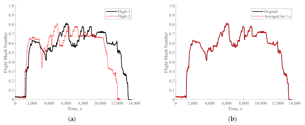
Figure 4a shows a representative flight history conducted at two different flights. It compares histories of the flight Mach numbers of the first flight (denoted as Flight 1) and second flight (denoted as Flight 2). Note that the first flight was the smooth wall case and the second flight was the wall case with riblets. Target cruise conditions were those in which the altitude was maintained for at least 60 s, such as those at 2500 s with Mach 0.65. The targeted flight conditions were determined by accounting for s+, as mentioned above, and several targeted conditions were made in a single flight. Therefore, the flight profile had several acceleration and deceleration scenarios, as shown in Figure 4a. Note that the figure shows the slight difference in flight-sequence scenarios between the first flight (used as reference case in a later section) and the second flight (used as compared case in a later section), such as the varying duration of maneuvers, ensuring that total flight durations were different. Despite the differences in time, a wide range of flight conditions was applied in each case.
Figure 4b shows the time history of the Mach number obtained on the same flight as that presented in Figure 4a for the first flight case. The original time-series data recorded at 10 Hz and time-averaged data made for a duration of 1 s are plotted. The 1-s-averaged data were identical to the original datasets, without any unexpected errors. Therefore, 1-s-averaged data are used for evaluations in this study. It should be noted that data averaged up to 10 s followed the trend of the original 10-Hz sampled data. However, since the main objective of this study is to draw a comparison between two different flights at near-identical times while reducing data scattering, 1-s averaging is employed for further post-processing.
3. Data-Reduction Methods
This section presents data-reduction techniques, including (i) an interpolation method based on the response surface methodology (RSM-based interpolation) and (ii) the proposed residual-norm-based interpolation to search for the closest flight conditions in time-series data among reference and compared cases.
3.1. Response Surface Methodology and Governing Parameters for RSM-Based Interpolation
As mentioned in the Introduction, flow features, such as boundary-layer profiles around the airframe, cannot always be the same as those of the target flight conditions due to the difference in remaining fuel, the resulting difference in the angle of attack, and the atmospheric conditions for each flight. The datasets of both cases would be obtained on different flights [32]. This leads to difficulties in repeatability of measurements of flight data. In order to perform a proper comparison for a dataset, such as boundary-layer profiles obtained from different flights to eliminate the influence of various flight conditions, an approach was taken to interpolate the data using response surface methodology. Details of the principle behind this application are described by Takahashi et al. [32]. Furthermore, a second-order response surface curve was chosen to improve the fitting accuracy [32], instead of the second-order fitting that is generally used [43].
In applying RSM to the interpolation of the boundary-layer profile, many combinations between the fitting order of the response surface model (N = 2, 3, 4, …) and the flight data (M∞, Re∞, α, etc.) may be possible. For instance, a sufficiently large number of datasets would increase the accuracy of the fitting curve in response surface model, using as many variables as possible. However, available data points would generally be limited, and some additional consideration was given to selecting the governing parameters.
In a previous study [32], the governing parameters responsible for reconstructing the pressure coefficient were selected as the flight Mach number and the total pressure, which were obtained by the onboard ADS, by accounting for Equation (4). The primary reasons for selecting these two variables were that the numerator of Equation (4) is the measured data, and the denominator is the flight data obtained by the ADS. Note that the uncertainty inherent in the air-data measurement was 0.025% for total pressure and 1.01% for Mach number, obtained as 1σ during constant Mach-number conditions in a range from Mach 0.4 to 0.8. The uncertainty is also described in Section 4.3. The static pressure was converted from the total pressure and Mach number assuming isentropic conditions. Since the pitot pressure is normalized by the flight data, the flight Mach number and total pressure that appear in the denominator evidently influence the scaling of Cp. Considering the measurement uncertainties for these parameters, this isentropic assumption can contain approximately 2.4% of uncertainty. Note that the application of these two variables to the RSM successfully interpolated the boundary layer profile with an uncertainty range of 4% [32]. A detailed discussion of the uncertainty is given in Section 4.1.
3.2. Interpolation of Boundary-Layer Profile
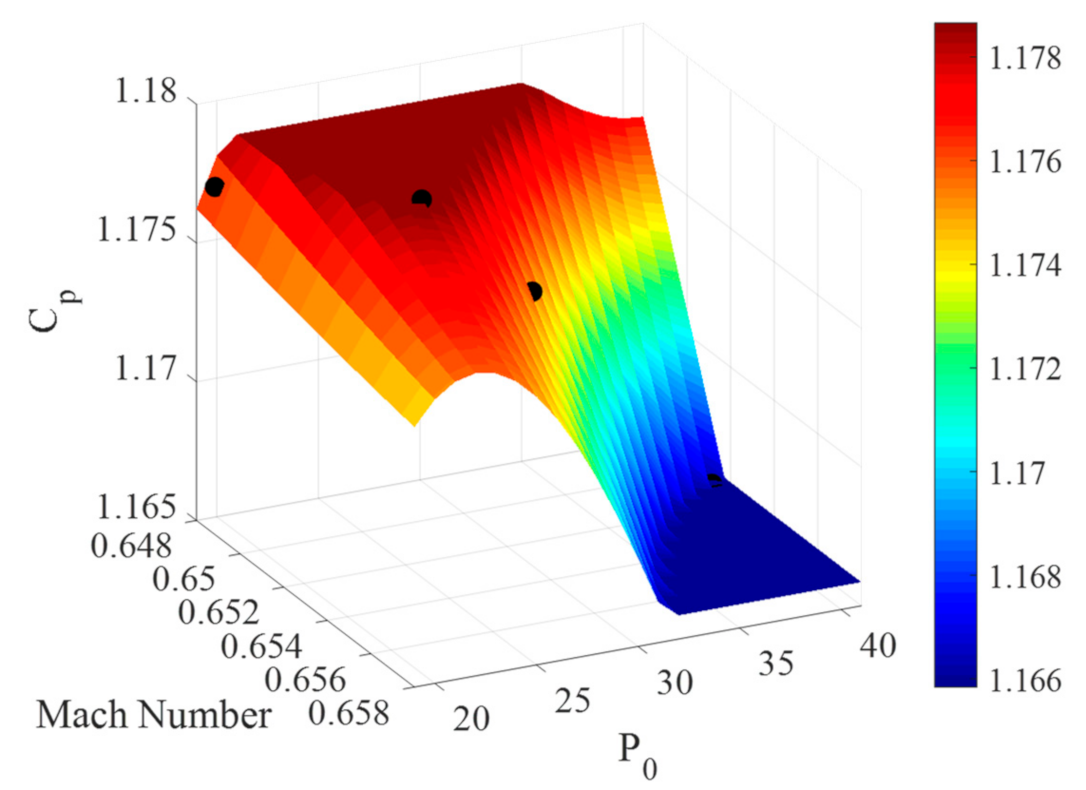
Figure 5 shows an example of the response surface model used to interpolate the boundary-layer profile in the compared case. The RSM model was reconstructed based on the Mach number and total pressure, as mentioned in Section 3.1. At each time instance, RSM was created based on the reference flight condition using data from a total of 45 probes for each flight condition. In Figure 5, the original experimental data are superimposed as black dots for comparison. The experimental data indicate the case for target Mach number of 0.65 and measured at probe number 45 (near the outer edge of the boundary layer). The corresponding response surface model for probe 45 is presented in this figure. The response surface model reconstructs the Cp distribution through the interpolation technique using RSM as a function of the Mach number and total pressure with good accuracy. The interpolation interval was 0.001 for Cp distribution, considering the significant digits for the ADS system. Similar to the previous method [32], the restriction was added to the interpolation to ensure that the generated response surface did not involve any extrapolations and to increase the accuracy. For example, if the Cp distribution made by the RSM method exceeds the boundary values determined by the Mach number and the total pressure, it is considered as an outlier and is limited to the boundary values of the constrained area [32]. This reconstruction is implemented at every Cp value of 0.001 that exceeds boundary values. This process strengthens the robustness of the interpolation as it ensures that only interpolation is used and prevents potential errors due to extrapolation.
3.3. Residual-Norm Calculation (Residual-Norm-Based Interpolation)
In this section, a method to identify the most closely matched flight conditions between the compared case and that of the reference case is presented. For a certain time instance of the reference case, all time instances in time-series data in a compared case are subject to searching for a combination of variables that makes the residual-norm value minimal. The identified time instance for the compared case that had the lowest residual-norm value was considered to be the condition corresponding to that of the reference case. The residual-norm value (r) between the reference and the compared cases was calculated using Equation (5).
where up to six variables (var), M∞, P0∞, T0∞, s+, α, and V∞ are considered.
These six variables (N = 6) cover every major condition during flight. The Mach number is also considered to evaluate the compressibility. In this study, up to six of these variables were chosen to identify the most closely matched flight conditions between the compared case and the reference case. It should be noted that these variables can be dependent variables. For example, Mach number and temperature are related to each other. Therefore, some information on some physical properties can be redundant in the norm calculation. However, since it is meaningful to consider the values that can represent flight conditions, this approach was taken. It should also be noted that weighted norm evaluation is also possible. However, standard variables are used in this study and weighted approach will be discussed in a future study.
4. Results and Discussion
This section discusses the insights gained from the RSM-based interpolation technique and the proposed norm-based interpolation technique, which cover the uncertainty and accuracy of interpolation for the flight experimental data measured during different flights.
4.1. Errors Associated with RSM-Based Interpolation
First, to show the effectiveness of the interpolation of the boundary-layer profile by using the RSM-based interpolation, one example case of a boundary layer profile is discussed in this section. Figure 6 compares the U- velocity profiles of representative reference and compared cases, obtained on different flights under the closest-matched flight conditions between the two flights (where “Ref” denotes flight conditions with M∞ = 0.75, α = 0.66°, and s+ = 18.5 and “Com” denotes flight conditions with M∞ = 0.70, α = 1.23°, s+ = 17.9). These flight conditions and data were found by using the residual-norm evaluation. The “original” and “interpolated” profiles denote the raw profile and interpolated profile, respectively. For example, in Figure 6, the label Ref (Original) represents the original boundary-layer-profile data for the reference case; and the data labeled Ref (Interpolated) represents the interpolated data for the reference case. The same rule is applied to the other dataset. The third-order response surface model with two variables, x1 = P0∞ and x2 = M∞, was employed here for the RSM-based interpolation [32]. It should be noted that the RSM-based interpolation aim to eliminate the differences in flight conditions. Therefore, if the premised conditions between two different flights are exactly the same, it is not necessary to implement the RSM-based interpolation.
As shown in Figure 6, it is trivial that the reconstructed interpolated curve for the reference case (Ref (Interpolated)) was identical to the original profile (Ref (Original)) since the same dataset was used for the interpolation. In Figure 6, the original profiles in the reference and compared cases were almost identical, especially around the outer edge, where the freestream velocity was measured. This indicates that there was no need to implement the RSM-based interpolation because the flights’ conditional differences had already been minimized by the residual-norm calculation.
Similar observations were obtained for datasets at other time instances. Therefore, the residual-norm calculation itself is sufficient to minimize the flight conditional difference. However, RSM-based interpolation may be needed in addition to this method to improve the accuracy. This is discussed in more detail in Section 4.2. The error level was calculated as 1.9%, which is described in detail in Section 4.3.
4.2. Influence of Parameter Selection on Case Identification
In Section 3.3, it was stated that up to six variables were considered in the residual-norm calculation. These six variables cover all the major flight conditions. It should be noted that a greater number of variables would have offered higher accuracy; however, since the residual norm would have displayed some sensitivity to the variables, the limited number of variables with high sensitivity were expected to allow the residual norm to be computed with higher accuracy. In order to ensure that the best combination of variables was obtained, the error associated with the selection of variables was evaluated. This evaluation is described here.
In the residual-norm calculation, the following procedure was followed. At a certain instance in the reference case, the residual-norm values for all the instances in the compared case were calculated by Equation (5). Next, the timepoint at which the residual-norm value was minimal was found in the compared case.
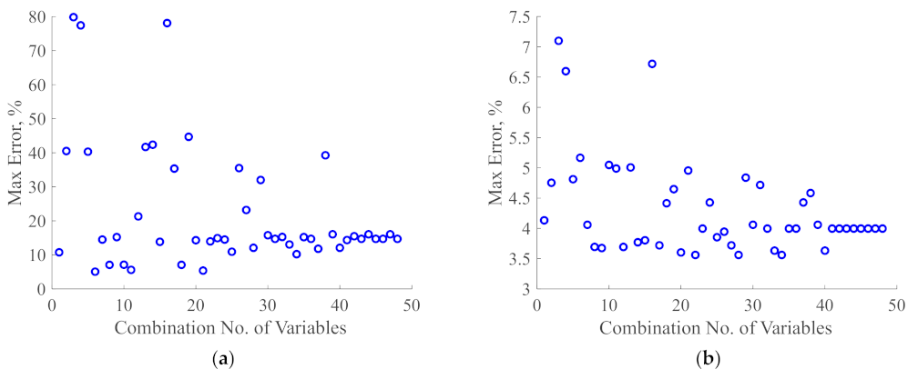
The maximum error associated with the residual-norm-calculation process obtained among the outer pitot probes (No. 44 and No. 45) between the reference and the compared cases for all the time-series data (at each 1-s averaged duration) is considered. Figure 7 shows the error levels (the average of maximum errors for the outer probes) for all the variable combinations (a) without RSM-based interpolation and (b) with RSM-based interpolation, in addition to the residual-norm interpolation. Obviously, the overall error level for the interpolation without RSM-based interpolation was large. In Figure 7a, three error level can be observed around 10–20%, 40%, and 80%. These different error levels resulted from the combinations of variables when calculating the norm. The obvious outliers appearing at around 80% of the error level were related to cases using only one variable of s+ or α for the norm calculation. The errors appearing around 40% were found to be cases in which the variables associated with flight velocity or Mach number were not used. It was found that the inclusion of the flight velocity or Mach number reduced the error levels to 10%. Figure 7b shows much lower levels of errors. Thus, the RSM-based interpolation is beneficial in reducing the overall error level for any combination of variables. The minimum value in the maximum error can be seen at the combination numbers of 22, 28, and 34 in Figure 7b. Since the use of more variables offers higher accuracy, combination No. 34, which gives a combination of four variables (M∞, P0∞, s+, and V∞), was chosen.
The flight conditions at this time instance for the compared case are now considered to be the case corresponding to the reference case’s time instance and are used to compare the boundary-layer profile in the next step.
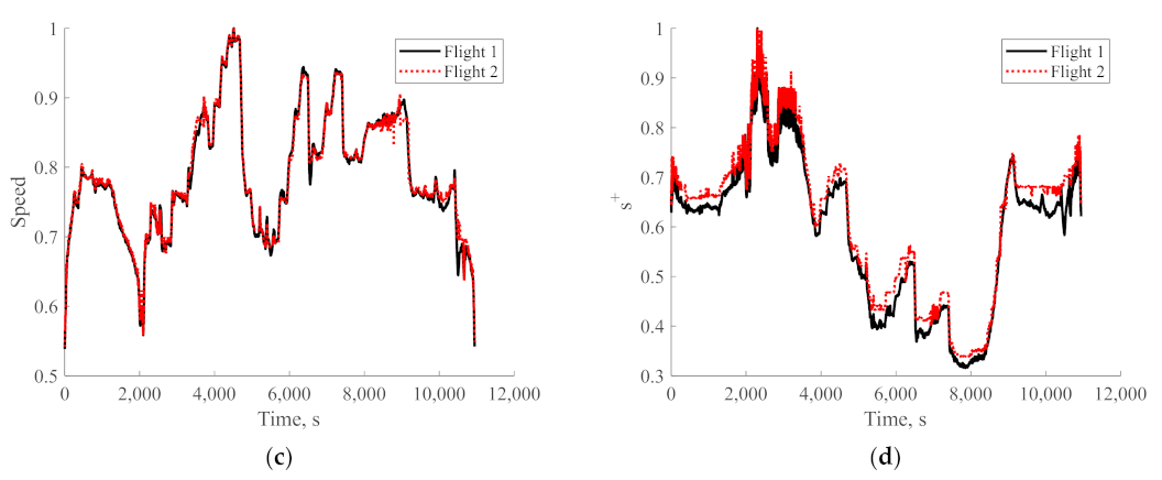
Figure 8 presents the time-series datasets of the measured data (solid line) and residual-norm-searched data (dotted line) for the Mach number, total pressure, flight speed, and s+. The solid lines correspond to the reference case (Flight 1) and the dotted lines (Flight 2) correspond to the compared case. Each parameter was normalized by its maximum value. The main reason for showing this plot is to show that the residual-norm approach can find the flight condition that is most closely matched to the reference data at each timepoint. According to Figure 4a, which shows original datasets for both cases, it is obvious that the total duration of the flight time for each case is different and, thus, each flight procedure is different. Accounting for this difference in flight procedure, the horizontal axis on each plot indicates the time starting from a timepoint at which the flight Mach number exceeded 0.4 in the ascent phase. This makes the comparison between these two different flights appropriate. It should be noted that the flight procedures for these two flights were not identical, but the difference was small because these two flights were intended to have the same flight conditions and procedures. The resulting datasets (dotted lines), which had the minimum norm values of the variables, showed good agreement with the reference data (solid lines). This fact also indicates that the differences in the testing duration had no influence on the residual-norm calculation and that the corresponding comparison data could be found throughout the testing scenario.
Again, it should be noted that the time index (instance) that had the lowest residual-norm value for the compared case was considered to provide the closest flight condition to that of the reference case in each instance. Furthermore, it should be noted that this search process was applied to the 1-s-averaged datasets or the almost-simultaneous datasets covering the entirety of the respective flights.
4.3. Errors Associated with the Residual-Norm Calculation
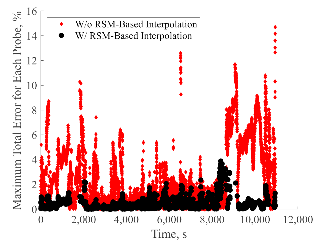
Next, the error levels associated with the norm calculation were evaluated. In order to calculate the error range associated with the norm-calculation process, the maximum errors obtained in the process among the outer pitot-probes (Nos. 44 and 45) between the reference and compared cases for all the time-series data (at each 1-s-averaged duration) are plotted in Figure 9. In addition to the norm-based interpolation, the results with and without the RSM-based interpolation were plotted. Each data point expresses the average difference in boundary-layer-velocity values between two flights. This error is associated with the boundary-layer velocities identified by the norm calculation. It should be noted, again, that the flight conditions of M∞ < 0.4 were eliminated before calculating the residual-norm procedure.
Takahashi et al. [32] stated that RSM-based interpolation significantly reduces error levels for similar applications. As in these other applications, the error level for the process with RSM-based interpolation became much smaller. The maximum errors with and without RSM-based interpolation were 14.7% and 3.9%, respectively. Therefore, residual-norm calculation with the RSM-based interpolation reduces the error level associated with flight conditional difference.
Next, the cumulative error associated with the residual-norm-based interpolation combined with the RSM-based interpolation is discussed. Table 1 summarizes the possible error sources inherent in both the measurement and the post-processing. Each measured value (flight data, including atmospheric data and pitot pressure) was averaged for 1 s. These associated errors were considered to be 1σ for each datum for the average duration, as mentioned in the previous section. As shown in Table 1, the error associated with the RSM-based interpolation described in the previous section was the governing source of errors. The rate of the cumulative error (total error) was approximately 5.7% with the RSM-based interpolation.
Thus, it is possible to interpolate the boundary-layer profile with this level of error by using the proposed residual-norm-calculation method combined with the RSM-based interpolation.
4.4. Application of the Interpolation Method to Evaluate u+ Gain by Riblets
In fact, the quantitative evaluation of the reduction in skin friction drag using riblets needs extremely accurate measurement and careful evaluation. Therefore, a level of uncertainty of 6% or greater is unacceptable for evaluating the skin-friction-drag reduction by riblets. In this regard, the error level of 5.7% as mentioned above is too large for the quantitative and effective evaluation of the reduction in skin friction drag. Additionally, a quantitative evaluation needs an additional calibration curve that converts such representative parameters as Δu+ (representing the skin friction drag to the quantitative skin-friction coefficient (cf)). However, this study does not contain any data such as calibration curves; hence, a quantitative evaluation is not possible within the scope of this study. Therefore, instead of evaluating the effect of riblets on the reduction in the skin friction drag in a quantitative manner, this section discusses the applicability of the proposed residual-norm-based interpolation method to evaluate the skin-friction-drag reduction in a qualitative manner.
To this end, the Δu+ or u+ gain when using riblets was calculated first. In order to calculate the Δu+ with the riblets, the focus was on the boundary-layer profile in the log-law region, where it usually appeared around y+ of 100–1000. To convert the boundary-layer profile in a log scale, the following y+- u+ plot was employed. The Δu+ is the reduction in skin friction drag. The Y+ and u+ were calculated from Equations (6)–(8).
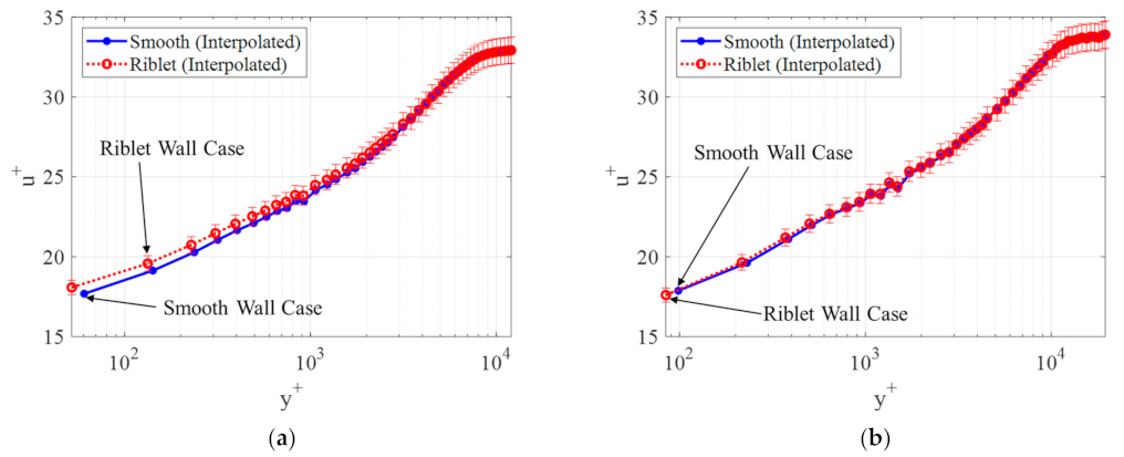
Figure 10 presents some representative u+-y+ plots for cases s+ of 17 and 31. The smooth-wall case and the riblet-wall case are compared. The error bar is 5.7% for u+, which was obtained from Table 1. The positive riblet effect is shown in Figure 10a at s+ = 17, where Δu+ is expected to be the maximum, as shown through the u+ gain in the region of y+ < 2000. The s+ = 31, which is shown in Figure 10b, is where Δu+ is expected to be negative or exert no positive effect, indicating that the riblet would reduce the skin-friction-drag reduction [30,44].
Since the log-law region was usually considered for a y+ of 100 to 1000, Δu+ at an average of y+ = 200–500 considering some data-scattering features was compared between the reference and compared cases.
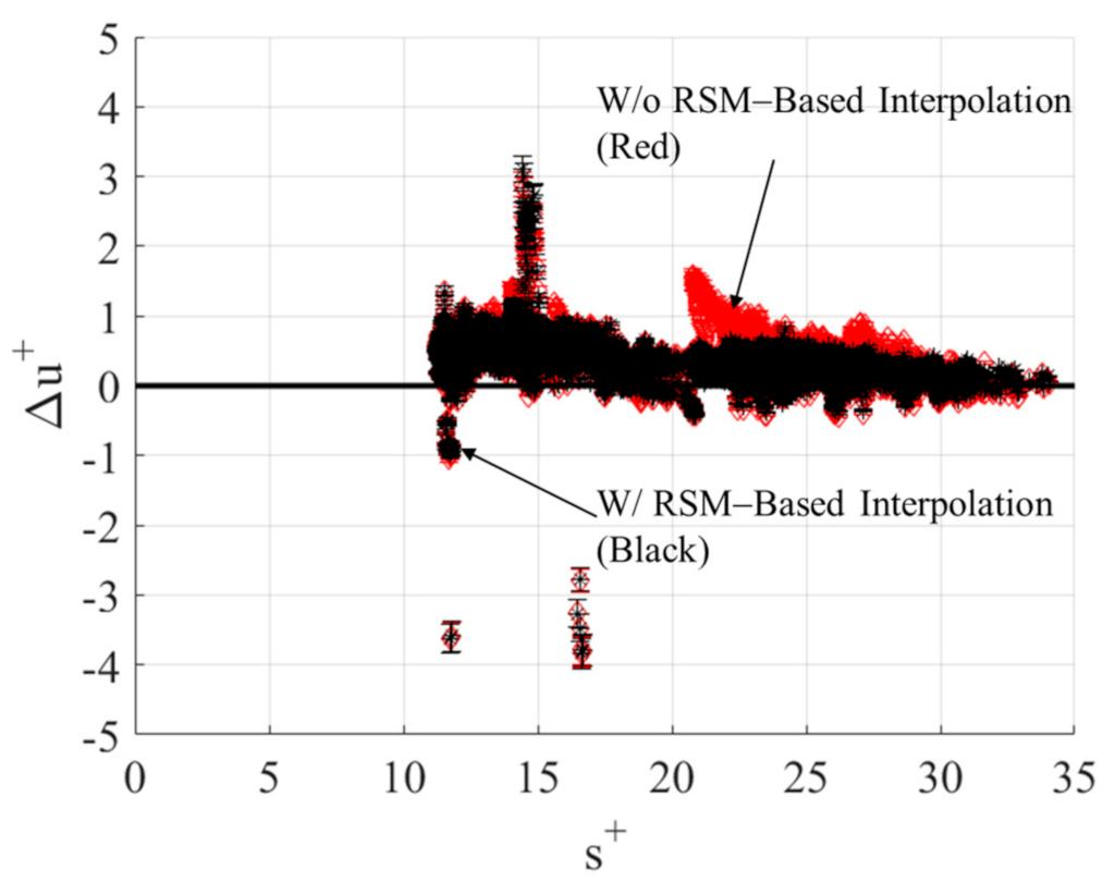
Figure 11 presents the resulting Δu+ plotted against the s+. The Δu+ obtained without using RSM-based interpolation (red) was compared with those with RSM-based interpolation (black). The error bar was 5.7%, as discussed in Section 4.3. The RSM-based interpolated datasets showed slightly less data scattering, although almost the same Δu+ was obtained throughout the s+ range.
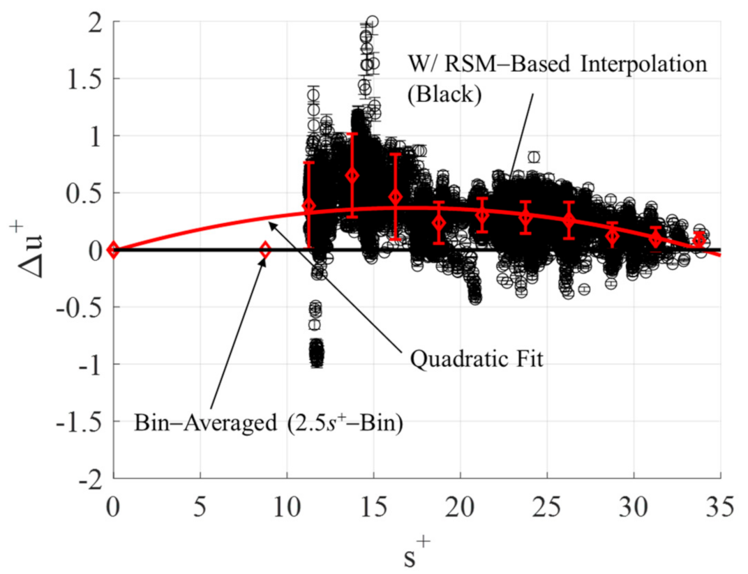
Figure 12 enlarges the Δu+ based on the datasets with RSM-based interpolation, shown in Figure 11, for the Δu+ range of −2 to 2, and also shows the bin-averaged Δu+ calculated with an s+ bin-range of 2.5s+. A quadratic curve fitted to the bin-averaged dataset is also superimposed in the figure. The designed riblets were expected to show their maximum performance in reducing skin friction drag around the s+ of 17 [30,44]. The curve fitting clearly indicates the expected performance trend, which suggests that the positive effect of skin friction reduction appears to peak in the s+ range of around 10 to 20. Although some data scattering remains, the positive values of Δu+ in the s+ range of 10–30 predominate over those in the negative values. In the region where the s+ ranges below 10 and above 30, a negative expected performance of the riblets is displayed, in that the skin friction drag increases. Thus, qualitatively, the findings here are significant in that the RSM-based interpolation reduces the error level, which makes the trend of the Δu+ clearer.
5. Conclusions
Turbulent boundary-layer profiles on an aircraft surface were measured by pitot rakes during flight experiments with high subsonic-Mach-number ranges. The flight testing was conducted as part of the JAXA’s FINE project, which aims to evaluate the use of the JAXA-designed paint-based riblet to reduce skin friction drag. The turbulent boundary-layer profiles were measured in the first flight (with a smooth wall) and in the second flight (with a wall with a riblet).
Since different flights have different flight sequences, it is not easy to compare boundary-layer profiles measured on different flights directly. Using one flight as a reference, this paper proposed a method to find the closest match between the conditions of the different flights at each timepoint. The proposed method was used to calculate the residual error in the time-series data between two different flights for a combination of variables: Mach number, total pressure, nondimensional riblet width, and flight velocity.
The accuracy of the proposed method was evaluated in addition to a previously proposed RSM-based interpolation technique, which was reported to have a 4% error for a Mach-number range of 0.5 to 0.78 [32]. The proposed method would have an error level of 5.7% for all time-series data in the Mach number ranges of 0.4 to 0.8, except near take-off and landing, when used in combination with the RSM-based interpolation
The applicability of the proposed interpolation method was determined by applying the method to evaluate the skin-friction reduction regarding the gain in u+ (Δu+) when using the riblets. The results showed that the Δu+ peaked in the nondimensional riblet width (s+) range of 10–20, which was around the designed values; and at the other s+ ranges, the effectiveness of the riblets in reducing skin friction drag was reduced, as expected.
Thus, the proposed method with the four variables successfully identified the closest-matched conditions between two flights for the measured boundary-layer profiles, with an error level of 5.7% in a Mach number range of 0.4–0.8. Additionally, its applicability to the qualitative evaluation of skin-friction reduction was shown.
Author Contributions
H.T. was responsible for the entire work from its conceptualization, the establishment of the methodology, the data analysis, and the entire writing of the original manuscript; M.K. managed the overall project and reviewed it; H.I. and S.K. worked on the wind-tunnel experiments and raw-data processing. All authors have read and agreed to the published version of the manuscript.
Funding
This research received no external funding.
Acknowledgments
This study was conducted as part of the Flight Investigation of Skin-Friction Reduction Eco-Coating (FINE) project by JAXA’s Aeronautical Technology Directorate. The authors wish to thank Masato Asai and Ayumi Inazawa at Tokyo Metropolitan University, Shihoko Endo and Kaoru Iwamoto at the Tokyo University of Agriculture and Technology, and Ryoko Shinohara at the O-WELL corporation for the riblet design. The authors would also like to acknowledge Atsushi Yasuda and Yukio Oizumi at Diamond Air Service, Inc., and Hiroshi Tomita, Ikuya Shirota, Hideki Sato, Ryoji Hirai, Masayuki Nagae, Takehiro Kumagai, Wataru Mukaidani, and Masayoshi Noguchi at JAXA for conducting the flight testing. Finally, the authors would like to thank Yoshikazu Makino and Kouichiro Tani for their insightful help in the research collaboration across the directorates.
Conflicts of Interest
The authors declare no conflict of interest.
Nomenclature
| cf | local skin-friction coefficient |
| Cf | total skin-friction coefficient |
| Cp | pressure coefficient |
| M | Mach number |
| q | uncertainty |
| r | Residual-norm value |
| R | gas constant |
| Re | Reynolds number |
| s | width of riblet, μm |
| s+ | non-dimensional width of riblet |
| T | temperature, K or °C |
| U | streamwise velocity component (U-velocity), m/s |
| uτ | friction velocity |
| x | coordinate in streamwise direction |
| α | angle of attack, deg |
| γ | specific heat ratio |
| μ | dynamic viscosity |
| ν | kinematic viscosity, m2/s |
| θ | boundary layer thickness, mm |
| ρ | density, kg/m3 |
| σ | standard deviation |
| Subscripts | |
| 0 | standard condition |
| com | compared case |
| flight | flight condition |
| i, j | index number |
| interpolated | interpolated data |
| pitot | pitot-rake data |
| ref | reference case |
| s | static condition |
| total | total value |
| var | variable |
| ∞ | freestream condition |
References
- Szodruch, J. Viscous Drag Reduction on Transport Aircraft. AIAA Paper 91-0685. In Proceedings of the 29th Aerospace Sciences Meeting, Reno, NV, USA, 7–10 January 1991. [Google Scholar] [CrossRef]
- Jimenez, H.; Mavris, D. Pareto-Optimal Aircraft Technology Study for Environmental Benefits with Multi-Objective Optimization. J. Aircr. 2017, 54, 1860–1876. [Google Scholar] [CrossRef] [Green Version]
- Yousefi, K.; Saleh, R. Three-dimensional suction flow control and suction jet length optimization of NACA 0012 wing. Meccanica 2015, 50, 1481–1494. [Google Scholar] [CrossRef]
- Zhang, Z.Y.; Zhang, W.L.; Chen, Z.; Sun, X.H.; Xia, C.C. Suction control of flow separation of a low-aspect-ratio wing at a low Reynolds number. Fluid Dyn. Res. 2018, 50, 065504. [Google Scholar] [CrossRef]
- Yousefi, K.; Saleh, R.; Zahedi, P. Numerical study of blowing and suction slot geometry optimization on NACA 0012 airfoil. J. Mech. Sci. Technol. 2014, 28, 1297–1310. [Google Scholar] [CrossRef] [Green Version]
- You, D.; Moin, P. Active control of flow separation over an airfoil using synthetic jets. J. Fluids Struct. 2008, 24, 1349–1357. [Google Scholar] [CrossRef]
- Wang, H.; Zhang, B.; Qiu, Q.; Xu, X. Flow control on the NREL S809 wind turbine airfoil using vortex generators. Energy 2017, 118, 1210–1221. [Google Scholar] [CrossRef]
- Nadesan, T.; Estruch-Samper, D. Wake Instability Behind Low-Profile “Convergent Riblet” Vortex Generators in Incompressible Laminar Flow. AIAA J. 2018, 56, 3008–3023. [Google Scholar] [CrossRef]
- Butt, F.R.; Talha, T. Numerical Investigation of the Effect of Leading-Edge Tubercles on Propeller Performance. J. Aircr. 2019, 56, 1014–1028. [Google Scholar] [CrossRef]
- Saravi, S.S.; Cheng, K.A. A Review of Drag Reduction by Riblets and Micro-Textures in the Turbulent Boundary Layers. Eur. Sci. J. 2013, 9, 62–81. [Google Scholar]
- Walsh, M.J. Riblets. In Viscous Drag Reduction in Boundary Layers; Bushnell, D.M., Hefner, J.N., Eds.; Progress in Astronautics and Aeronautics; AIAA: New York, NY, USA, 1989; Volume 123, pp. 203–261. [Google Scholar]
- Walsh, M.J. Riblets as a Viscous Drag Reduction Technique. AIAA J. 1983, 21, 485–486. [Google Scholar] [CrossRef]
- Sareen, A.; Deters, R.W.; Henry, S.P.; Selig, M.S. Drag Reduction Using Riblet Film Applied to Airfoils for Wind Turbines. J. Sol. Energy Eng. 2014, 136, 021007. [Google Scholar] [CrossRef]
- Raayai-Ardakani, S.; McKinley, G.H. Drag reduction using wrinkled surfaces in high Reynolds number laminar boundary layer flows. Phys. Fluids 2017, 29, 093605. [Google Scholar] [CrossRef] [Green Version]
- Sasamori, M.; Iihama, O.; Mamori, H.; Iwamoto, K.; Murata, A. Parametric Study on a Sinusoidal Riblet for Drag Reduction by Direct Numerical Simulation. Appl. Sci. Res. 2017, 99, 47–69. [Google Scholar] [CrossRef]
- Bushnell, D.M.; Hefner, J.N.; Ash, R.L. Effect of compliant wall motion on turbulent boundary layers. Phys. Fluids 1977, 20, S31–S48. [Google Scholar] [CrossRef]
- Suzuki, Y.; Kasagi, N. Turbulent drag reduction mechanism above a riblet surface. AIAA J. 1994, 32, 1781–1790. [Google Scholar] [CrossRef]
- Dean, B.; Bhushan, B. Shark-Skin Surfaces for Fluid-Drag Reduction in Turbulent Flow: A Review. Philos. Trans. R. Soc. A 2010, 368, 4775–4806. [Google Scholar] [CrossRef] [Green Version]
- Viswanath, P.R. Aircraft viscous drag reduction using riblets. Prog. Aerosp. Sci. 2002, 38, 571–600. [Google Scholar] [CrossRef] [Green Version]
- Mele, B.; Tognaccini, R.; Catalano, P. Performance Assessment of a Transonic Wing–Body Configuration with Riblets Installed. J. Aircr. 2015, 53, 129–140. [Google Scholar] [CrossRef] [Green Version]
- Catalano, P.; de Rosa, D.; Mele, B.; Tognaccini, R.; Moens, F. Performance Improvements of a Regional Aircraft by Riblets and Natural Laminar Flow. J. Aircr. 2020, 57, 29–40. [Google Scholar] [CrossRef]
- Xu, Y.; Song, W.; Zhao, D. Efficient Optimization of Ringlets for Drag Reduction over the Complete Mission Profile. AIAA J. 2018, 56, 1483–1494. [Google Scholar] [CrossRef]
- Okabayashi, K.; Matsue, T.; Asai, M. Development of Turbulence Model to Simulate Drag Reducing Effects of Riblets. J. Jpn. Soc. Aeronaut. Space Sci. 2016, 64, 41–49. (In Japanese) [Google Scholar] [CrossRef]
- Sawyer, W.; Winter, K. An Investigation of the Effect on Turbulent Skin Friction of Surface with Streamwise Grooves. In Proceedings of the International Conference on Turbulent Drag Reduction by Passive Means, The Royal Aeronautical Society, London, UK, 15–17 September 1987; Volume 2, pp. 330A–362A. [Google Scholar]
- Walsh, M.J. Turbulent Boundary Layer Drag Reduction Using Riblets. AIAA Paper 82-0169. In Proceedings of the 20th Aerospace Sciences Meeting, Orlando, FL, USA, 11–14 January 1982. [Google Scholar] [CrossRef]
- Bechert, D.W.; Bruse, M.; Hage, W.; Van Der Hoeven, J.G.T.; Hoppe, G. Experiments on drag-reducing surfaces and their optimization with an adjustable geometry. J. Fluid Mech. 1997, 338, 59–87. [Google Scholar] [CrossRef]
- MBB Transport Aircraft Group. Microscopic Rib Profiles Will Increase Aircraft Economy in Flight. Aircr. Eng. Aerosp. Technol. 1988, 60, 11. [Google Scholar] [CrossRef]
- Kurita, M.; Nishizawa, A.; Okabayashi, K.; Koga, S.; Kwak, T.; Nakakita, K.; Naka, Y. FINE: Flight Investigation of Skin-Friction Reducing Eco-Coating. In Proceedings of the 54th Aircraft Symposium, The Japan Society for Aeronautical and Space Sciences, JSASS-2016-5180, Tokyo, Japan, 24–26 October 2016. (In Japanese). [Google Scholar]
- Koga, S.; Kurita, M.; Iijima, H.; Okabayashi, K.; Nishizawa, A.; Takahashi, H.; Endo, S. Wind Tunnel Tests for Measurement System Design of Flight Investigation of Skin-Friction Reducing Eco-Coating (FINE). In Proceedings of the 54th Aircraft Symposium, The Japan Society for Aeronautical and Space Sciences, JSASS-2016-5105, Tokyo, Japan, 24–26 October 2016. (In Japanese). [Google Scholar]
- Kurita, M.; Iijima, H.; Koga, S.; Nishizawa, A.; Kwak, D.; Iijima, Y.; Takahashi, H.; Abe, H. Flight Test for Paint-Riblet. AIAA Paper-2020-0560. In Proceedings of the AIAA Scitech 2020 Forum, Orlando, FL, USA, 6–10 January 2020. [Google Scholar] [CrossRef]
- Available online: http://www.aero.jaxa.jp/eng/publication/magazine/sora/2011_no40/ss2011no40_03.html (accessed on 27 January 2021).
- Takahashi, H.; Kurita, M.; Iijima, H.; Sasamori, M. Interpolation of Turbulent Boundary Layer Profiles Measured in Flight Using Response Surface Methodology. Appl. Sci. 2018, 8, 2320. [Google Scholar] [CrossRef] [Green Version]
- Rosenbaum, B.; Schulz, V. Response Surface Methods for Efficient Aerodynamic Surrogate Models. Computational Flight Testing. 2013, 123, 113–129. [Google Scholar] [CrossRef]
- Sevant, N.E.; Bloor, M.I.G.; Wilson, M.J. Aerodynamic Design of a Flying Wing Using Response Surface Methodology. J. Aircr. 2000, 37, 562–569. [Google Scholar] [CrossRef]
- Zhang, M.; He, L. Combining Shaping and Flow Control for Aerodynamic Optimization. AIAA J. 2015, 53, 888–901. [Google Scholar] [CrossRef]
- Papila, M.; Haftka, R.T. Response Surface Approximations: Noise, Error Repair, and Modeling Errors. AIAA J. 2000, 38, 2336–2343. [Google Scholar] [CrossRef]
- Madsen, J.I.; Shyy, W.; Haftka, R.T. Response Surface Techniques for Diffuser Shape Optimization. AIAA J. 2000, 38, 1512–1518. [Google Scholar] [CrossRef]
- Walsh, M.J.; Sellers, W.L.; McGinley, C.B.; Sellers, I.W.L. Riblet drag at flight conditions. J. Aircr. 1989, 26, 570–575. [Google Scholar] [CrossRef]
- Walsh, M.J.; Sellers, I.W.L.; Mcginley, C.B. Riblet Drag Reduction at Flight Conditions. AIAA Paper 88-2554. In Proceedings of 6th Applied Aerodynamics Conference, Williamsburg, VA, USA, 6–8 January 1988. [Google Scholar] [CrossRef]
- Mclean, J.D.; George-Falvey, D.N.; Sullivan, P.P. Flight Test of Turbulent Skin-Friction Reduction by Riblets. In Proceedings of the International Conference on Turbulent Drag Reduction by Passive Means, The Royal Aeronautical Society, London, UK, 15–17 September 1987; pp. 408–424. [Google Scholar]
- Larson, T.J. Evaluation of a Flow Direction Probe and a Pitot-Static Probe on the F-14 Airplane at High Angles of Attack and Sideslip; NASA Technical Memorandum 84911. Report No. NASA-TM-8491; NASA: Washington, DC, USA, 1984. [Google Scholar]
- Kurita, M.; Nishizawa, A.; Kwak, D.; Iijima, H.; Iijima, Y.; Takahashi, H.; Sasamori, M.; Abe, H.; Koga, S.; Nakakita, K. Flight Test of a Paint-Riblet for Reducing Skin-Friction. In Proceedings of the 2018 Applied Aerodynamics Conference, AIAA Paper 2018–3005. Atlanta, GA, USA, 25–29 June 2018. [Google Scholar] [CrossRef]
- Khuri, A.I.; Mukhopadhyay, S. Response surface methodology. WIREs Comput. Stat. 2010, 2, 128–149. [Google Scholar] [CrossRef]
- Iijima, H.; Takahashi, H.; Koga, S.; Sasamori, M.; Iijima, Y.; Abe, H.; Nishizawa, A.; Kurita, M. Skin Friction Drag Reduction in Turbulent Boundary Layer Conditions over Riblet Surfaces. In Proceedings of the AIAA Scitech 2019 Forum, AIAA-2019-1621. San Diego, CA, USA, 7–11 January 2019. [Google Scholar] [CrossRef]
Figure 1.
The JAXA flight-test bed and paint-based riblet surface attached to the aircraft: (a) Flight-test bed; (b) mounted pitot rakes.
Figure 1.
The JAXA flight-test bed and paint-based riblet surface attached to the aircraft: (a) Flight-test bed; (b) mounted pitot rakes.

Figure 2.
A photograph presenting a cross-sectional plane of the riblet.

Figure 3.
Relationship between s+ and unit Reynolds number for: (a) on-design (target) cruise conditions; (b) all conditions from time-series data over Mach 0.4.
Figure 3.
Relationship between s+ and unit Reynolds number for: (a) on-design (target) cruise conditions; (b) all conditions from time-series data over Mach 0.4.

Figure 4.
Representative flight history showing Mach number: (a) Original flight histories for two flights; (b) original and 1-s-averaged flight histories for the smooth wall.
Figure 4.
Representative flight history showing Mach number: (a) Original flight histories for two flights; (b) original and 1-s-averaged flight histories for the smooth wall.

Figure 5.
Data interpolation using the response surface model reconstructed per Mach number and total pressure (original experimental data are superimposed as black dots for comparison).
Figure 5.
Data interpolation using the response surface model reconstructed per Mach number and total pressure (original experimental data are superimposed as black dots for comparison).

Figure 6.
Example case (M∞ = 0.73, α = 0.78°, P∞ = 42.0 kPa, T∞ = 221.6 K) of the original velocity profiles superimposed with the interpolated profiles.
Figure 6.
Example case (M∞ = 0.73, α = 0.78°, P∞ = 42.0 kPa, T∞ = 221.6 K) of the original velocity profiles superimposed with the interpolated profiles.

Figure 7.
Average of maximum percentage errors presented for outer pitot probes (nos. 44 and 45) for all measured flight cases (a) without RSM-based interpolation and (b) with RSM-based interpolation.
Figure 7.
Average of maximum percentage errors presented for outer pitot probes (nos. 44 and 45) for all measured flight cases (a) without RSM-based interpolation and (b) with RSM-based interpolation.

Figure 8.
Time-series datasets comparing each reference and compared case found by residual-norm calculations with four variables: (a) M∞; (b) P0∞; (c) V∞; and (d) s+. Each variable was normalized by its maximum value.
Figure 8.
Time-series datasets comparing each reference and compared case found by residual-norm calculations with four variables: (a) M∞; (b) P0∞; (c) V∞; and (d) s+. Each variable was normalized by its maximum value.


Figure 9.
Maximum percentage uncertainty for all pitot probes for all measured flight cases caused by interpolation.
Figure 9.
Maximum percentage uncertainty for all pitot probes for all measured flight cases caused by interpolation.

Figure 10.
Comparison of boundary-layer profiles between smooth-wall and riblet-wall cases at (a) a near design point (s+ = 17) and (b) an off-design point (s+ = 31).
Figure 10.
Comparison of boundary-layer profiles between smooth-wall and riblet-wall cases at (a) a near design point (s+ = 17) and (b) an off-design point (s+ = 31).

Figure 11.
Resulting Δu+ obtained from methods with and without RSM-based interpolation.

Figure 12.
Enlarged Δu+ obtained from RSM-based interpolated data, bin-averaged Δu+, and their curve fits.
Figure 12.
Enlarged Δu+ obtained from RSM-based interpolated data, bin-averaged Δu+, and their curve fits.


Table 1.
Summary of possible uncertainty sources with or without RSM-based interpolation.
| Uncertainty Source | Symbol | Value, % | Note |
|---|---|---|---|
| Total pressure | q1 | 0.025 | Atmospheric air pressure measured by the onboard air-data-sensing system. |
| Mach number | q2 | 1.01 | Obtained by the onboard air-data-sensing system. |
| Pitot measurement | q3 | 3.5 | Max. percentage error obtained as 1σ over an averaged value for 1-min duration for all probes. |
| Response surface methodology (RSM) (interpolation) | q4 | 1.9 | When RSM-based interpolation is used. |
| Residual-norm calculation | q5 | 3.9 | Errors obtained from Figure 9, including pitot-pressure-measurement errors. |
| Total error | qtotal | 5.7 | With RSM-based interpolation. |
Disclaimer/Publisher’s Note: The statements, opinions and data contained in all publications are solely those of the individual author(s) and contributor(s) and not of MDPI and/or the editor(s). MDPI and/or the editor(s) disclaim responsibility for any injury to people or property resulting from any ideas, methods, instructions or products referred to in the content. |
© 2023 by the authors. Licensee MDPI, Basel, Switzerland. This article is an open access article distributed under the terms and conditions of the Creative Commons Attribution (CC BY) license (https://creativecommons.org/licenses/by/4.0/).
Share and Cite
MDPI and ACS Style
Takahashi, H.; Kurita, M.; Iijima, H.; Koga, S. Time-Series-Data Interpolation Applied to Boundary-Layer Profiles Measured on Different Flights. Aerospace 2023, 10, 322. https://doi.org/10.3390/aerospace10040322
AMA Style
Takahashi H, Kurita M, Iijima H, Koga S. Time-Series-Data Interpolation Applied to Boundary-Layer Profiles Measured on Different Flights. Aerospace. 2023; 10(4):322. https://doi.org/10.3390/aerospace10040322
Chicago/Turabian StyleTakahashi, Hidemi, Mitsuru Kurita, Hidetoshi Iijima, and Seigo Koga. 2023. "Time-Series-Data Interpolation Applied to Boundary-Layer Profiles Measured on Different Flights" Aerospace 10, no. 4: 322. https://doi.org/10.3390/aerospace10040322
Note that from the first issue of 2016, this journal uses article numbers instead of page numbers. See further details here.