RANS-Based Aeroacoustic Global Sensitivity Study and Optimization of UAV Propellers

Abstract

Modeling of Unmanned Aerial Vehicles (UAV) propellers in a global, multidisciplinary aeroacoustic optimization was investigated. The modeling consists of three aspects: geometry, aerodynamics, and aeroacoustics. Firstly, a parametric geometry model was established using chord, twist, and sweep distributions along the radius, defined by splines to ensure smoothness. Additionally, airfoil parameters including maximum camber and its position, as well as the position of maximum thickness, were added. Secondly, a blade geometry-resolved aerodynamic model based on steady RANS was established. A two-equation SST turbulence model was used for compressible flow with periodic boundary conditions. Thirdly, an aeroacoustic model for far-field tonal noise calculation was defined, based on the Ffowcs Williams and Hawkings analogy and a RANS solution. A global sensitivity analysis was performed to establish the importance of individual design variables. Consequently, surrogate modeling-based optimization strategy was devised to efficiently establish Pareto front of propeller geometries in multi-objective aeroacoustic optimization.

1. Introduction

Unmanned aerial vehicles (UAVs), especially multirotors with vertical take-off capabilities, have a number of applications, such as infrastructure inspections, agriculture, surveillance, delivery, and many others [1,2]. One of the reasons preventing their use, especially in urban areas, is the excessive, irritating noise [3], which may have a detrimental impact on health [4]. The main sources of multirotor noise are:

• propeller tonal and broadband noise, resulting from rotating motion, pressure variations, and turbulence (airfoil self-noise),
• noise from interactions: blade vortex interactions (BVI), interactions of propeller wake with structure, as well as wake–wake interactions.

System-level noise reduction is a complex, multidisciplinary task, involving not only purely aerodynamic design, but also novel ideas, such as the use of blade phasing or active control [3]. The computational cost of a high-fidelity analysis of system-level noise is very high. On a subsystem level, the most significant noise source is the rotating propeller. Consequently, the reduction of propeller noise is a sensible way of approaching the UAV noise problem.

Typical propeller noise mitigation strategies are concentrated on propeller size and shape optimization, including global parameters such as propeller radius and the number of blades, and local parameters, such as the chord, twist, and sweep distributions along the radius. Less conventional noise mitigation strategies are focused on a broadband noise minimization by the means of leading and trailing edge serrations, boundary layer tripping, or porous inserts [5]. Additionally, bio-inspired solutions may be considered, such as the mechanisms of noise reduction developed by owls [6]. These methods are a subject of ongoing research.

Traditional cheap, low-fidelity methods, such as methods based on the Blade Element Theory (BET)—typically coupled with 2D methods, providing local airfoil aerodynamics—are commonly used for propeller aerodynamic design and optimization [7]. Coupled with compact monopole/dipole Ffowcs Williams and Hawkings (FWH) formulations for noise calculation, these approaches provide reasonable tonal noise prediction, and can be successfully used to design quiet propellers [8,9,10]. Their limitations are related to the simplicity of the methods used. Especially in case of the low-Reynolds number propeller modeling, the broadband noise component should be accounted for, as its magnitude may be similar to that of the tonal component [11]. Low-fidelity semi-empirical wall-pressure spectrum models [12] may be used to calculate the broadband noise contribution of the turbulent boundary layer for a number of sections along the radius. The high-fidelity approach for Computational Aeroacoustics (CAA) involves a scale-resolving Computational Fluid Dynamics (CFD) model, such as Large Eddy Simulation (LES), hybrid RANS-LES, wall-modeled LES [13], or the Lattice–Boltzmann Method [14]. These inherently unsteady methods, however, cannot be considered in the optimization context due to their prohibitive computational cost.

While the low-fidelity methods are well-established in propeller design and optimization, the use of higher-fidelity methods becomes an intuitive next step to achieve more effective results. Adjoint [15] and global Surrogate-Based Optimization (SBO) [16] frameworks have been utilized in RANS-based optimization. Blade-resolved CFD methods can resolve the aerodynamics of a generic propeller, taking into account various global and local geometry features (which are often not captured with low-fidelity methods). Consequently, the actual, Computer-Aided Design (CAD)-based geometry parametrization can be used for optimization, without relying on the tip-loss model or other sources of error of the low-fidelity methods.

In propeller optimization with a fixed radius and number of blades, the remaining geometry features consist of chords, twists, and airfoils along the stacking line. A common choice of geometric parameters consists of chord and twist distributions along the radius. Sweep and thickness are often added to allow additional design freedom. 15-variable spline-based parametrization (five parameters for the chord, twist and sweep distributions each) was successfully used in aeroacoustic optimization [10]. In [17], the parametric model of the blade was built using variable: chord, twist, sweep and dihedral at three radial locations along the blade. While the shape of airfoils is typically less influential in terms of aerodynamic performance than the platform parameters, it can be optimized either in a single process, or in a separate step—after completing the platform design [7]. The latter process reduces the dimensionality of the optimization problem.

Sensitivity analysis—commonly divided into local and global—describes relations between input and output uncertainties [18]. Local sensitivity is described by derivatives at a point of interest. Global sensitivity requires information in the whole range of input variables, and allows thorough analysis of a system, including quantification of parameter influence on the output, as well as identification of interactions between parameters. In the optimization context, global sensitivity analysis quantifies the importance of variables on the objective function. Hence, it allows us to remove unimportant variables, tune bounds, and eventually build efficient parametric models. In surrogate-based optimization, such information might be available from the surrogate model, e.g., if the surrogate model is based on an anisotropic kernel. An example of this approach was presented on a wing design case study [19], where tuned kriging hyperparameters were used to assess the relative importance of geometric parameters. Where the interactions between parameters are sought, a global sensitivity study should be performed. A method allowing more in-depth understanding of global sensitivity is the method of variance decomposition [20], leading to the Sobol’ indices-based analysis. This approach was used to determine the relative influence of parameters in aerodynamic propeller optimization [21] and in an airfoil optimization for improved dynamic stall behavior, and therefore to determine parameters of the highest importance [22]. Sensitivity analyses—usually not considered for optimization problems described in the literature—provide valuable information, which can be used in future design cases.

In the current work, a comprehensive analysis of propeller modeling was performed, with emphasis on the setup of the optimization process. Blade geometry-resolved CFD is considered to allow for accurate modeling of a rotor in hover without assumptions regarding its geometry and performance. The selection of a parametric model was discussed based on a global sensitivity analysis. Finally, SBO was performed to validate the approach and draw final conclusions. The paper is structured as follows. The description of the methodology for SBO and the global sensitivity analysis is given in Section 2. A geometry parametric model, as well as the aerodynamic and aeroacoustic computational models, are described in Section 3. A global sensitivity analysis is outlined in Section 4, whereas the results of multi-objective optimization are described in Section 5. Finally, the conclusions are stated in Section 6.

2. Methodology

2.1. Global Optimization Using Surrogate Modeling

An optimization problem is typically formulated as a minimization of an objective function J:

$$\begin{array}{cc}\hfill \mathrm{minimize}:& J\left(\mathbf{x}\right)\hfill \\ \hfill \mathrm{with}\mathrm{respect}\mathrm{to}:& \mathbf{x}\hfill \\ \hfill \mathrm{subject}\mathrm{to}:& g\le 0\hfill \\ \hfill & h=0\hfill \\ \hfill & \mathbf{l}\le \mathbf{x}\le \mathbf{u}\hfill \end{array}$$

(1)

where g and h are inequality and equality constraints, and $\mathbf{x}$ is bounded between $\mathbf{l}$ and $\mathbf{u}$. The process of finding $\mathbf{x}$ for which $J\left(\mathbf{x}\right)$ is minimum, depends on many factors, including the cost of computing J, the number of variables, the objective function landscape, etc. In the current work, global optimization is considered, with continuous design variables. The objective function output is assumed to be smooth, which is typically the case for subsonic aerodynamics-related problems. The cost of a single evaluation of J is sufficiently high to rule out classic global optimization methods, such as direct optimization driven by an evolutionary algorithm. On the other hand, the potential complexity (multimodality) of the search space rules out the use of local optimizers, which are likely to get stuck in a local minimum.

The use of surrogate modeling-driven optimization allows the use of global search methods, which use cheap surrogate prediction instead of direct calls to J. A general procedure for SBO, presented schematically in Figure 1, is:

• Define an initial sample of points ($\mathbf{X}={[{\mathbf{x}}_0,{\mathbf{x}}_1,\dots ,{\mathbf{x}}_k]}^T$) in the search space. Run analysis of the initial sample to obtain the required output $\mathbf{y}$. In this work, both aerodynamic and aeroacoustic metrics are calculated from a CFD/CAA model.
• Train a surrogate model with the available data (the initial sample and infill points). Assess surrogate model quality (e.g., by cross validation).
• Find candidate point(s) for verification. The selection of candidates is typically performed by exploration and exploitation of the search space using global search methods.
• Verify candidate(s). Check process convergence/termination criteria—if not reached go back to step 2.

The initial sample required for a high quality surrogate model requires a uniform spread of candidate points in the search space. The Latin hypercube approach is often suggested [23], in which the value of a variable does not repeat in the sample. In the current work, the Latin hypercube approach was used, along with optimal a space-filling criterion [24].

The surrogate modeling methods and infill criteria used in the current work are based on kriging and follow from the efficiency of Efficient Global Optimization (EGO) [25].

Kriging

The presented kriging description is based on, and available in more detail in [26]. In order to model the statistical relationship between two points ${\mathbf{x}}_i$ and ${\mathbf{x}}_j$, the distance $\left|\right|{\mathbf{x}}_i-{\mathbf{x}}_j\left|\right|$ is considered. If small, the random variables $Y\left({\mathbf{x}}_i\right)$ and $Y\left({\mathbf{x}}_j\right)$ will be highly correlated. In kriging, the correlation function is defined as:

$$Corr\left[Y\left({\mathbf{x}}_i\right),Y\left({\mathbf{x}}_j\right)\right]=exp\left(-\sum _{l=1}^d{\theta }_l{|{\mathbf{x}}_{il}-{\mathbf{x}}_{jl}|}^{p_l}\right).$$

(2)

The use of such basis functions allows for the variance to be controlled in each dimension (the rate of correlation decrease) using the hyperparameter ${\theta }_l$. Additionally, the hyperparameter $p_l$ allows for the control of the smoothness of interpolation. Setting $p_l=2$ reduces the cost of model tuning, and can be used if the response surface is smooth. With initial sample data, the surrogate is trained by searching for hyperparameters, which maximizes the concentrated likelihood function:

$$-\frac{n}{2}\ln \left({\widehat{\sigma }}^2\right)-\frac{1}{2}\ln \left(\left|\mathbf{R}\right|\right),$$

(3)

where the mean is:

$$\widehat{\mu }=\frac{{\mathbf{1}}^T{\mathbf{R}}^{-1}\mathbf{y}}{{\mathbf{1}}^T{\mathbf{R}}^{-1}\mathbf{1}},$$

(4)

and the variance:

$${\widehat{\sigma }}^2=\frac{{(\mathbf{y}-\mathbf{1}\widehat{\mu })}^T{\mathbf{R}}^{-1}(\mathbf{y}-\mathbf{1}\widehat{\mu })}{n}.$$

(5)

The $n\times n$ correlation matrix $\mathbf{R}$ is calculated using Equation (2) for a set of observations $\mathbf{y}$. The process of tuning hyperparameters is the expensive part of surrogate model generation, especially for complex problems with large, multidimensional data sets. Eventually, the kriging surrogate allows to find the output at any point $\mathbf{x}*$, using the kriging predictor:

$$\widehat{y}\left(\mathbf{x}*\right)=\widehat{\mu }+{\mathbf{r}}^{\prime }{\mathbf{R}}^{-1}(\mathbf{y}-\mathbf{1}\widehat{\mu }).$$

(6)

The kriging prediction error is:

$$s^2\left(\mathbf{x}*\right)={\widehat{\sigma }}^2\left[1-{\mathbf{r}}^{\prime }{\mathbf{R}}^{-1}\mathbf{r}+\frac{{(1-{\mathbf{r}}^{\prime }{\mathbf{R}}^{-1}\mathbf{r})}^2}{{\mathbf{1}}^{\prime }{\mathbf{R}}^{-1}\mathbf{1}}\right],$$

(7)

which is zero at the sampled locations and grows when moving away. Thus, Equations (6) and (7) give a powerful tool for driving the optimization by providing cheap prediction of the output along with the associated error. The error is often used in the infill criterion

$$EI=y\Phi \left(\frac{y}{s\left(\mathbf{x}\right)}\right)+s\varphi \left(\frac{y}{s\left(\mathbf{x}\right)}\right)$$

(8)

where $y=y_{min}-\widehat{y}\left(\mathbf{x}\right)$.

The accuracy of a surrogate model prediction is assessed using Mean Sqaured Error (MSE) and Mean Average Error (MAE) metrics, calculated for the unseen test sample, defined by:

$$MSE=\frac{1}{n_{\mathrm{test}}}\sum _{i=1}^{n_{\mathrm{test}}}{(y_{\mathrm{test}}^i-{\widehat{y}}^i)}^2$$

(9)

$$MAE=\frac{1}{n_{\mathrm{test}}}\sum _{i=1}^{n_{\mathrm{test}}}|y_{\mathrm{test}}^i-{\widehat{y}}^i|$$

(10)

where $n_{\mathrm{test}}$ is the size of a testing set.

2.2. Sensitivity Analysis

The relative influence of parameters on the objective function (or other model output) was established using global sensitivity analysis. In this work, the method of variance decomposition was used to calculate Sobol’ indices [27]. The decomposition of the function $\mathit{Y}=f\left(\mathbf{x}\right)$ in terms of increasing dimensionality, where $\mathbf{x}$ is the set of design variables, is:

$$f\left(\mathbf{x}\right)=f_0+\sum _{i=1}^n{f}_i\left(x_i\right)+\sum _{1\le i\le j\le n}^n{f}_{ij}(x_i,x_j)+...+f_{12\dots k}(x_1,x_2,\dots ,x_n),$$

(11)

where $f_0$ is a constant, and $f_i$, $f_{ij}$, and $f_{ij\cdots k}$ are the first, second, and kth-order functions, respectively, defined as:

$$f_0=\mathbb{E}\left(\mathit{Y}\right),$$

(12)

$$f_i=\mathbb{E}\left(\mathit{Y}\right|x_i)-\mathbb{E}\left(\mathit{Y}\right),$$

(13)

$$f_{ij}=\mathbb{E}\left(\mathit{Y}\right|x_i,x_j)-f_i-f_j-\mathbb{E}\left(\mathit{Y}\right).$$

(14)

Calculation of the conditional expectation $\mathbb{E}\left(\mathit{Y}\right|x_i)$ was performed by separating $x_i$ from the domain and taking the average of $\mathit{Y}|x_i$. The variation of $\mathbb{E}\left(\mathit{Y}\right|x_i)$ across $x_i$ is therefore a measure of sensitivity—if large, $x_i$ is important. The total variance of $\mathit{Y}$ is:

$$\mathbb{V}\left(\mathit{Y}\right)=\sum _i^n{V}_i+\sum _i^n\sum _{i<j}^n{V}_{ij}+\cdots +V_{12\dots n},$$

(15)

where $V_i=\mathbb{V}\left[\mathbb{E}\left(\mathit{Y}\right|x_i)\right]$. The Sobol’ first-order index is:

$$S_i=\frac{{\mathit{V}}_i}{\mathbb{V}\left(\mathit{Y}\right)},$$

(16)

while the total-effect Sobol’index is:

$$S_{T_i}=1-\frac{\mathbb{V}\left(\mathbb{E}\left(\mathit{Y}\right|{\mathbf{x}}_{\sim i})\right)}{\mathbb{V}\left(\mathit{Y}\right)},$$

(17)

where ${\mathbf{x}}_{\sim i}$ is the set of all variables except $x_i$.

In order to understand and draw conclusions from a Sobol’ indices-based sensitivity analysis, their key properties are summarized:

• $S_{T_i}\ge S_i$. The difference $S_{T_i}-S_i$ quantifies the level of interactions with other variables. If $S_{T_i}=S_i$, the variable $x_i$ does not interact with other variables.
• If $S_{T_i}$ is close to zero, $x_i$ can be assumed to have a negligible influence on the output. In the optimization context, $x_i$ can be fixed or removed from the set of variables.

The procedure of computing Sobol’ indices is performed with a Monte Carlo-based procedure, as described in [20].

3. Computational Modeling

The need for blade-resolved CFD used in this study was dictated by two factors. Firstly, the hover operating conditions imply strong interaction of the flow around the blade with the wake of the preceding blade. These three-dimensional phenomena require appropriate modeling, which rules out the use of cheap blade element-based methods. While comparisons between low and high-fidelity models can be performed [28] to establish sources of low-fideity errors, the use of high-fidelity codes remains inevitable. Secondly, the optimization perspective implies the method must be robust and give accurate results for different input geometries. As a consequence, the simplified methods—based on the two-dimensional airfoil data [29]—give correct results only in a limited operating regime. The modeling approach presented in this section aimed to exploit advantages of blade-resolved CFD while keeping the computational cost as low as possible.

The modeling consists of three parts: geometry, aerodynamics, and aeroacoustics. The first describes the parametric model of a blade geometry. Then, a CFD model of the resulting geometry was built, which includes meshing, analysis, and postprocessing. Finally, noise emission was calculated at specified observer locations, using input from the aerodynamic model and the FWH analogy.

3.1. Geometry

A parametric model of a propeller blade is defined by airfoil stacking, based on:

• distributions of chord, twist, and sweep along the radius, and
• local airfoil shape (changing along the radius).

The chord, twist, and sweep distributions along the radius were defined using a spline-based approach. Parameters define the positions of knots, giving smooth distributions, with direct control over values at the first and last sections. The number of knots and the extent of their freedom of movement remain arbitrary decisions, with different choices documented in the literature, as was discussed in Section 1. Typically, up to five knots were used, often fixed at selected positions along the radius to reduce the optimization problem dimensionality.

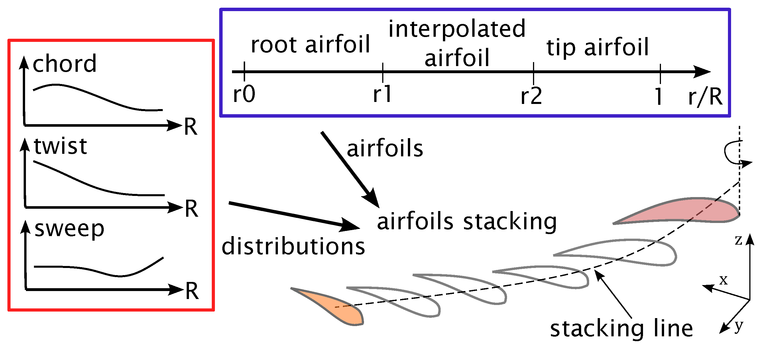
Local airfoil shape was defined using two baseline airfoils: root and tip airfoils. The blade was divided into three segments along the radius: the inward segment with the root airfoil, the outward with the tip airfoil, and the transitional—with an interpolated airfoil. This is presented in Figure 2, with parameters $r0$, $r1$, and $r2$ defining bounds for successive segments. The airfoils were stacked with a reference point at 40% chord along the stacking line, defined by the sweep distribution. The stacking line lies in the xy-plane, i.e., there is no dihedral. Finally, the airfoils stacking was calculated. The airfoil at a desired radial position is either the root or tip airfoil, or is found by linear interpolation of the two. The summary of the parametric model is presented in Figure 2. The dense stacking of airfoils along the stacking line—defined by the sweep distribution—was used to define a three-dimensional CAD model of the blade.

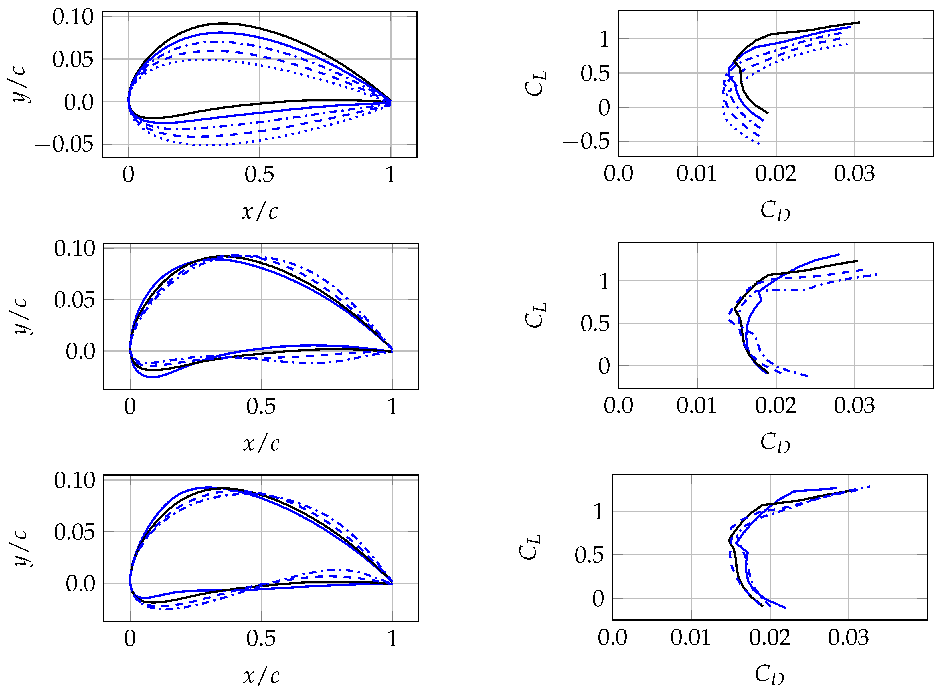
Airfoil parametrization aimed to allow major modifications to airfoil properties with as few parameters as possible. Consequently, the parametric model was built on a baseline airfoil, with modifications to maximum camber value and chordwise positions of maximum camber and thickness. The modification of these parameters allowed us to exploit a relatively large design space. Figure 3 presents the example effect of the described modifications on the NACA4412 airfoil scaled to 10% thickness. Three perturbation types are presented: maximum camber change, maximum camber position change, and maximum thickness position change. The resulting airfoils are presented in the left column, whereas the corresponding XFOIL predictions, performed at $Re=1.0\times {10}^5$, are presented in the right column. The camber modification gives the capability of achieving the desired $C_L$ at a minimum $C_D$. The maximum camber and thickness positions are parameters changing the behavior of the lift–drag curve. It should be emphasized that not only may the three presented airfoil modifications occur simultaneously, but also that the chord and twist distributions are subject to a global optimization. What is more, the rotating motion of the propeller blade is complex and—especially in the tip region—might result in operating conditions that cannot be captured with two-dimensional airfoil analysis.

3.2. Aerodynamics

This section describes the specification of the CFD model used in the current work, including the mesh independence study. The thrust ($C_T$) and torque ($C_Q$) coefficients of a propeller are:

$$C_T=\frac{T}{{\rho }_{\infty }\pi {\Omega }^2{R}^4}$$

(18)

$$C_Q=\frac{Q}{{\rho }_{\infty }\pi {\Omega }^2{R}^5}$$

(19)

where ${\rho }_{\infty }$ is the freestream density, $\Omega$ is the rotational speed in radians per second, and R is the tip radius. The hover performance is defined by the Figure of Merit (FM):

$$\mathrm{FM}=\frac{P_i}{P}=\frac{1}{\sqrt{2}}\frac{C_T^{1.5}}{C_Q}$$

(20)

where $P_i/P$ is the ideal power to the actual power ratio, for convenience written in terms of force coefficients.

Finite volume Reynolds-Averaged Navier–Stokes (RANS) equations with eddy-viscosity $k-\omega$ SST turbulence model were selected for aerodynamics modeling [30].

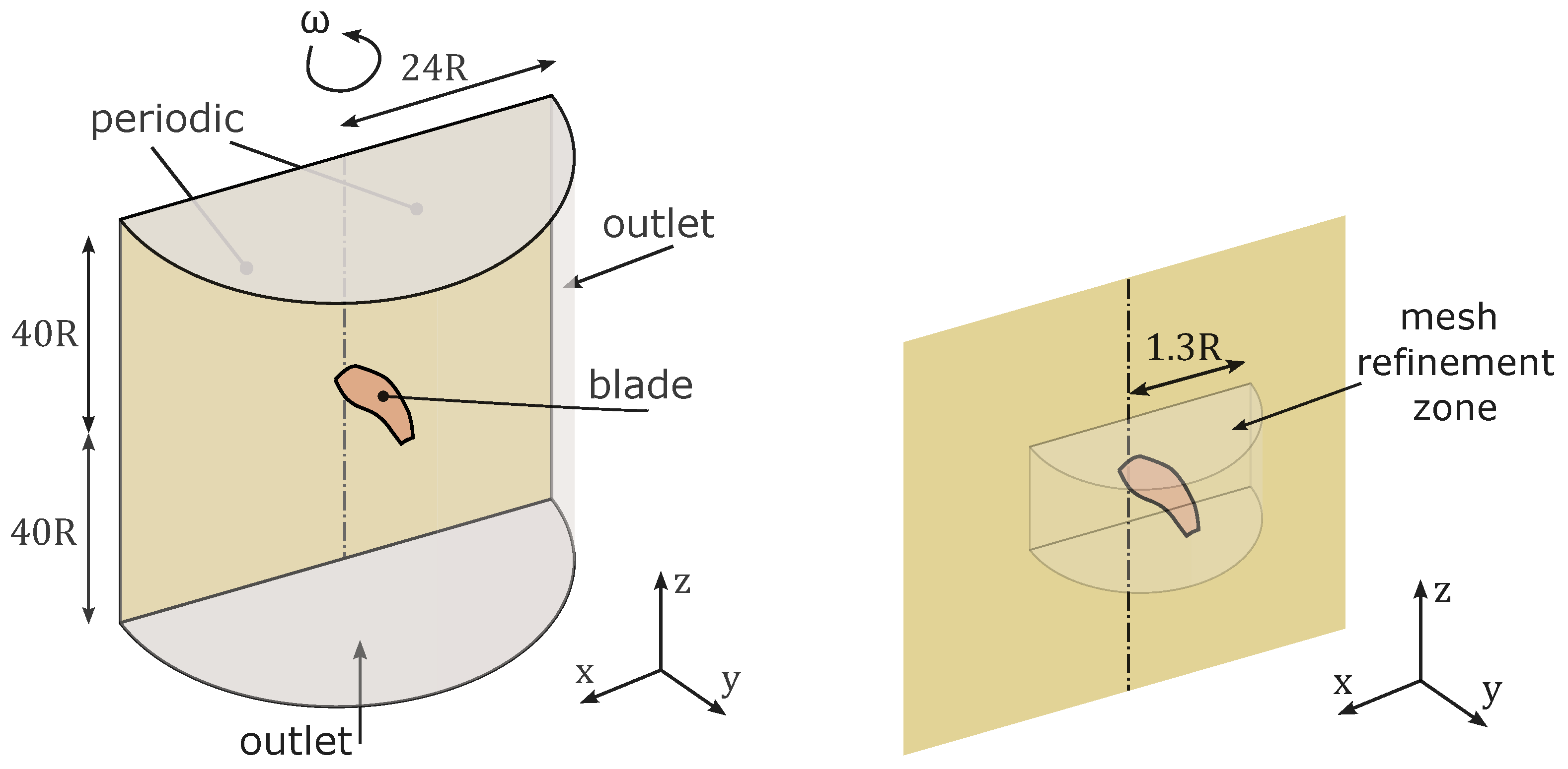
The computational model of a single blade was used, due to the periodic nature of isolated propeller analysis. The computational domain extends 24 radii in the blade direction and 40 radii in the upstream and downstream directions. A single rotating reference frame approach was used to model the propeller rotation. Hover was modeled with pressure–outlet boundary conditions on the non-periodic boundaries of the domain. The setup is presented schematically in Figure 4.

A compressible, coupled pressure-based solver was used with the second order pressure interpolation scheme. The second order-upwind scheme was used for spatial discretization of convection terms. The under-relaxation was controlled by a pseudo-transient approach. With a solution typically converging after around 2000 iterations, an additional 1000 iterations were added to allow for the averaging of a statistically steady solution.

An unstructured, polyhedral meshing procedure was established to provide case-independent quality of solutions. The mesh sizing was defined by a combination of local and global metrics, including maximum angle and minimum size (for surface meshes) and body-of-influence type refinement regions around the blade (volume meshes). 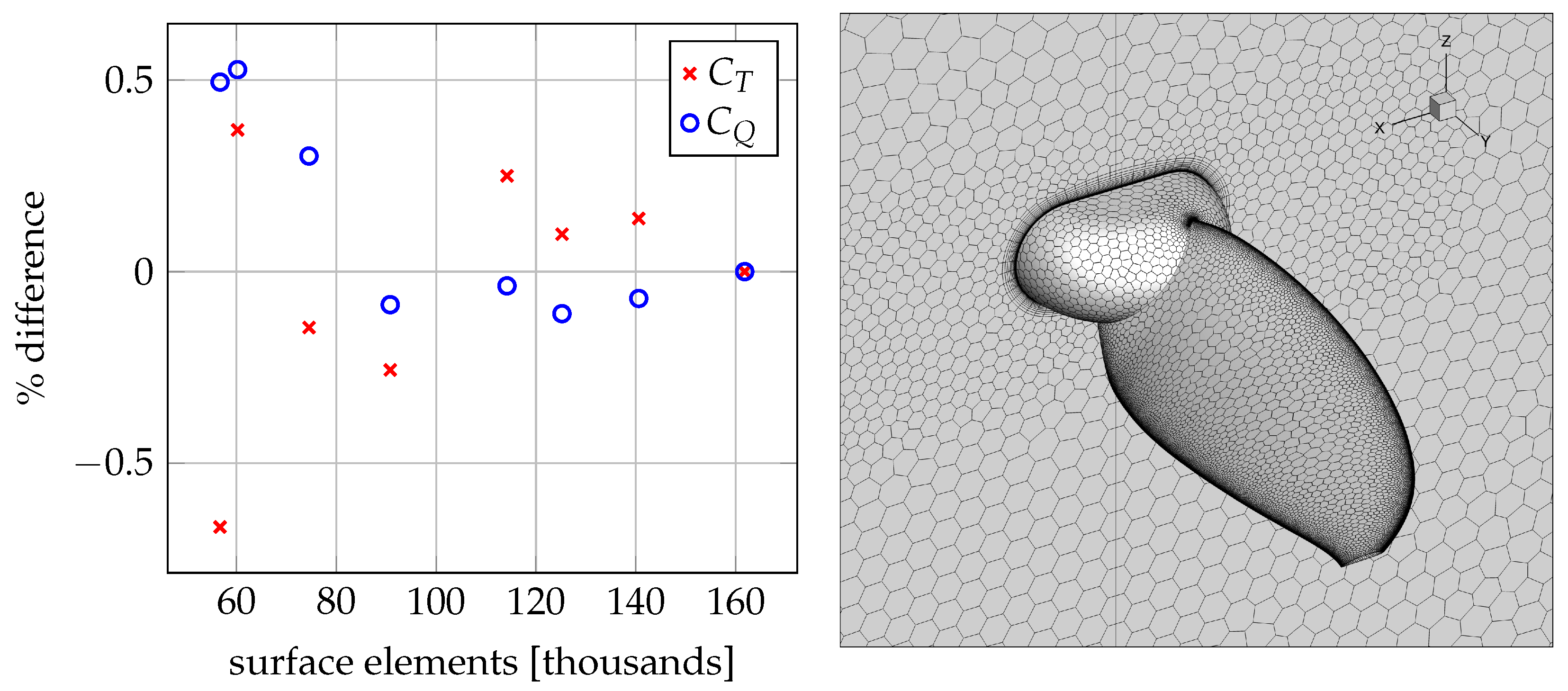The near-wall prism thickness was established to ensure $y^{+}$ in the viscous sub-layer regime, i.e., $y^{+}\le 5$, while the number of layers was dictated by the need for smooth transition to unstructured polyhedral. The growth ratio was fixed at 1.18. The mesh independence study included both surface and volume mesh settings. Firstly, an independent surface mesh was established by varying maximum angle (between neighboring elements) and minimum size. Then, the volume mesh settings were established, which defined the number of prism layers and refinement sizing. The resulting area-weighted average of $y^{+}$ was around a unity with 24 prism layers. The summary of the mesh independence study is presented in Figure 5. The left plot presents the surface mesh convergence, while the right figure presents an example surface mesh on the blade surface, as well as the effect of volume refinement visible on the periodic surface. In surface mesh sizing, the mesh with around 115 thousand elements was deemed sufficient (the number of elements is case-dependent). The final volume mesh size was between 3.5 to 4 million elements.

Both meshing and CFD were performed using commercial software Ansys Fluent 21.1. The computational time of a single case (meshing and CFD) was between 5 to 6 h using 24 processes.

3.3. Aeroacoustics

The aeroacoustic performance is characterized by the overall sound pressure level (OASPL):

$$\mathrm{OASPL}=20{log}_{10}\frac{p_{\mathrm{rms}}}{p_0},$$

(21)

where $p_{\mathrm{rms}}$ is the root-mean-square sound pressure and $p_0$ = 2 × 10⁻⁵ Pa is the reference pressure. The OASPL uses acoustic pressure fluctuations to determine the equivalent sound level. A frequency weighting can be used to adjust the OASPL to account for the influence of relative loudness perceived by the human ear, which is less sensitive to low and high frequencies.

The pressure signal required to find the OASPL at a selected observer location was calculated using the Farassat 1A formulation (F1A) [31] of FWH acoustic analogy [32], based on the solution of the RANS CFD model. In this approach, the blade is rotated virtually and the pressure distribution on the blade surface is constant. Only tonal noise is captured with this approach, as there are no pressure oscillations resulting from turbulence. Ansys Fluent [33] was used to calculate acoustic signals using the retarded time approach. To ensure sufficient sampling for the tonal noise calculation, acoustic signal was collected 40 times per revolution for 30 revolutions.

3.4. Model Validation

A literature-based benchmark of a two-bladed, 30 cm-diameter propeller [34] was used to validate the computational methods described in this section. The propeller geometry has a constant NACA4412 airfoil (12% thickness) along the radius. The experiments were conducted in an anechoic wind tunnel, at several advance ratios, including hover.

Table 1. Thrust, torque, and the resulting FM for the benchmark propeller.

Method	${\mathit{C}}_{\mathit{T}}$	${\mathit{C}}_{\mathit{Q}}$	FM
experiment	0.01505	0.00195	0.669
CFD	0.01524	0.00218	0.611

presents a comparison of thrust and torque obtained experimentally and calculated using CFD. While the thrust prediction is very close to the experiment, torque is significantly higher, which results in a significantly smaller FM. Similar results were obtained using a high-fidelity Lattice–Boltzmann Method in the literature benchmark. A major drawback of the current computational model is the assumption of a fully turbulent flow and boundary layer. 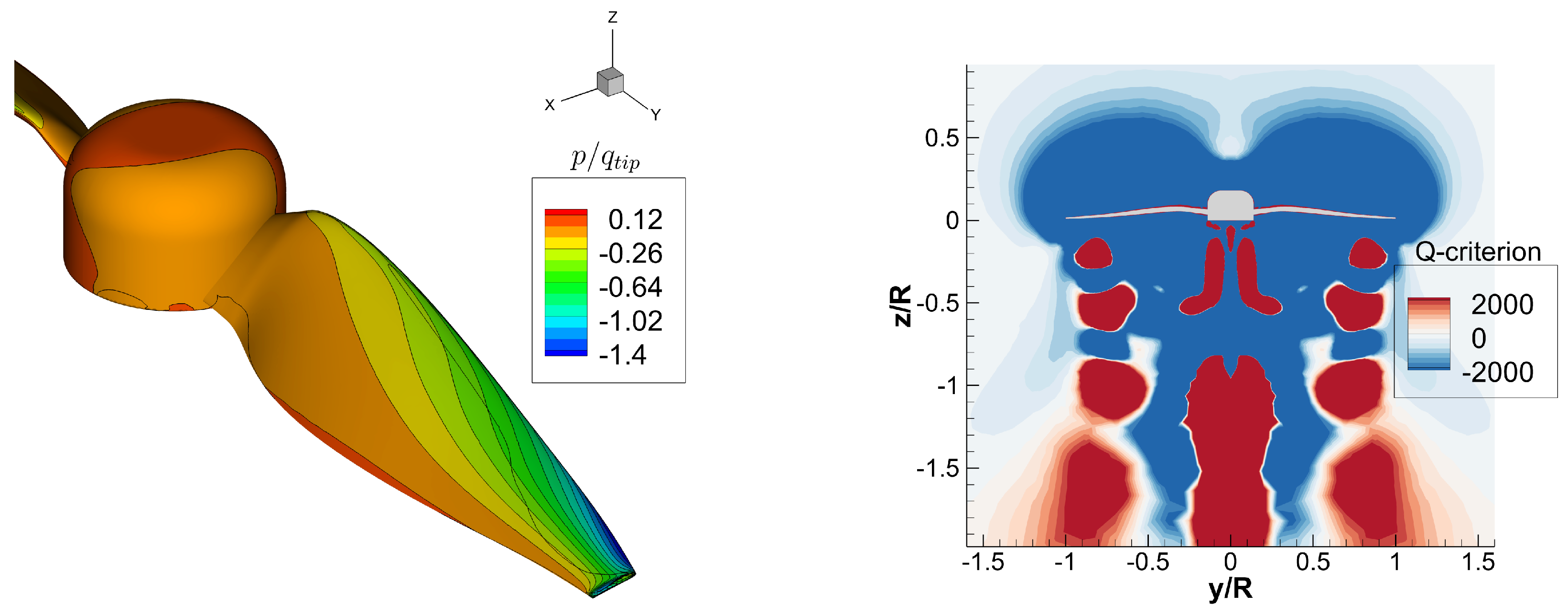The differences reported in Table 1 can be partly attributed to this simplification. Nevertheless, in the optimization context of the current work, the predictive capabilities of the model were deemed sufficient. An example of CFD results is visualized in Figure 6, including a pressure distribution (nondimensionalized by tip dynamic pressure) and a q-criterion map depicting the wake path downstream of the propeller. The proximity of preceding-blade wake and its potential interaction with the blade is shown (the preceding-blade wake is the red area centered around $0.2R$ below the blade tip region).

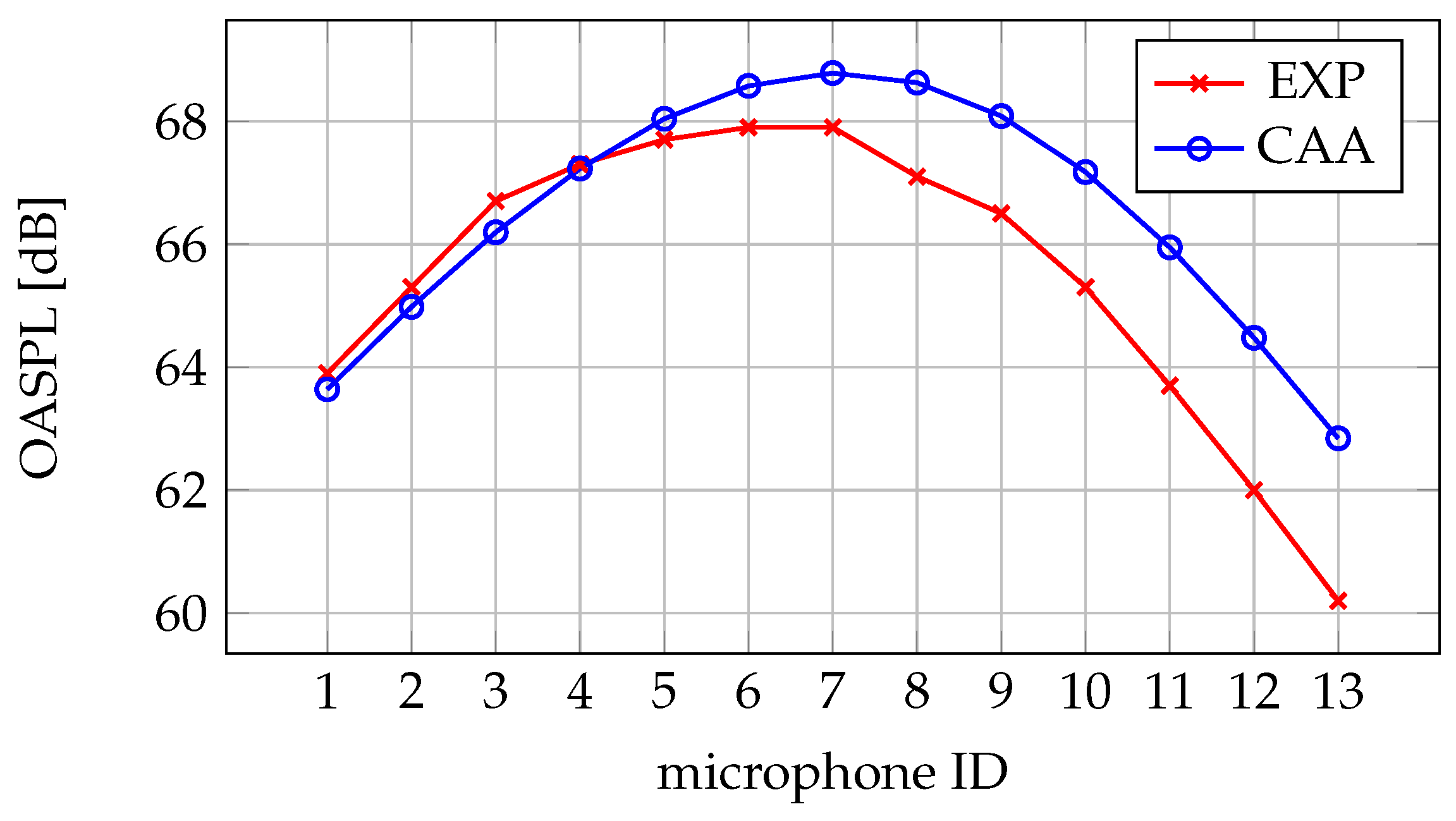
The noise prediction validation is presented in Figure 7. The experimental setup consisted of 13 uniformly distributed microphones located in a line $1.2$ $\mathrm{m}$ (four propeller diameters) away from the rotation axis. Microphones are numbered from 1 to 13, from the most downstream microphone 1 located $0.9$ $\mathrm{m}$ below the plane of rotation, through the in-plane microphone 7, up to the most upstream microphone 13 located $0.9$ $\mathrm{m}$ above the plane of rotation. A very good agreement between experimental and CAA results was obtained for microphones downstream of the propeller, with increasing discrepancy as the observation point moves upstream. The trends are correctly captured with the highest OASPL at microphone 7 and lower values upstream than downstream. Given the simplicity of the computational method, along with the aforementioned simplification in turbulence modeling, this result is satisfactory.

4. Initial Sample and Sensitivity Analysis

In the current work, a propeller of $0.3$ m diameter (i.e., $R=0.15\mathrm{m}$) with 8 N of hover thrust was sought. The initial sample was defined using an optimized Latin hypercube approach, as stated in Section 2. The parameter bounds are stated in

Table 2. The lower (l) and upper (u) bounds of parameters.

ID	Parameter	l	u	ID	Parameter	l	u
0	$c_0$	0.03	0.045	10	$s_2$	−0.0025	0.0075
1	$c_1$	0.03	0.06	11	$s_3$	$s_2-0.0025$	$s_2+0.01$
2	$c_2$	0.02	0.04	12	$s_4$	$s_3-0.0025$	$s_3+0.01$
3	$c_3$	$c_4$	2.5$c_4$	13	$r_1$	0.3	0.6
4	$c_4$	0.005	0.016	14	$ca{m}_{\mathrm{root},\mathrm{val}}$	0	0.06
5	${\beta }_0$	30	45	15	$ca{m}_{\mathrm{root},\mathrm{pos}}$	0.3	0.6
6	${\beta }_1$	15	35	16	$t_{\mathrm{root},\mathrm{pos}}$	0.2	0.5
7	${\beta }_2$	${\beta }_3$	${\beta }_3+6$	17	$ca{m}_{\mathrm{tip},\mathrm{val}}$	0	0.06
8	${\beta }_3$	8	18	18	$ca{m}_{\mathrm{tip},\mathrm{pos}}$	0.3	0.6
9	${\beta }_4$	${\beta }_3-5$	${\beta }_3+1$	19	$t_{\mathrm{tip},\mathrm{pos}}$	0.2	0.5
				20	$\omega$	4200	5000

. The radial locations of knots defining chords and twists are given by $\mathbf{r}=[0.2,r_1,0.8,0.93,1]\times R$. The airfoil segments coincide with these locations, i.e., the root airfoil, was kept between $0.2R-r_{1}R$, the tip airfoil between $0.93R-1R$, and the interpolated airfoil in the middle segment. The maximum airfoil thickness was fixed at 10% chord (constant along the blade). The near-tip region refinement (i.e., the three knots within 20% of the blade tip) was established to allow more design freedom in the most sensitive part of the blade. Chords (c) and sweeps (s) are given in meters, twists ($\beta$) are given in degrees, the second knot radial position ($r_1$) is given as a fraction of radius, and camber values ($ca{m}_{\_,\mathrm{val}}$) and positions of maximum camber ($ca{m}_{\_,\mathrm{pos}}$) and thickness ($t_{\_,\mathrm{pos}}$) are given as a local chord fraction. The relative values of lower ($\mathbf{l}$) and upper ($\mathbf{u}$) bounds for $c_4$, ${\beta }_2$, ${\beta }_4$, and sweep parameters were used to maintain the blade tip geometry for a given set of parameters. Finally, the rotational speed ($\omega$) was defined in revolutions per minute (rpm). The indices of chords, twists, and sweeps parameters increase towards the blade tip.

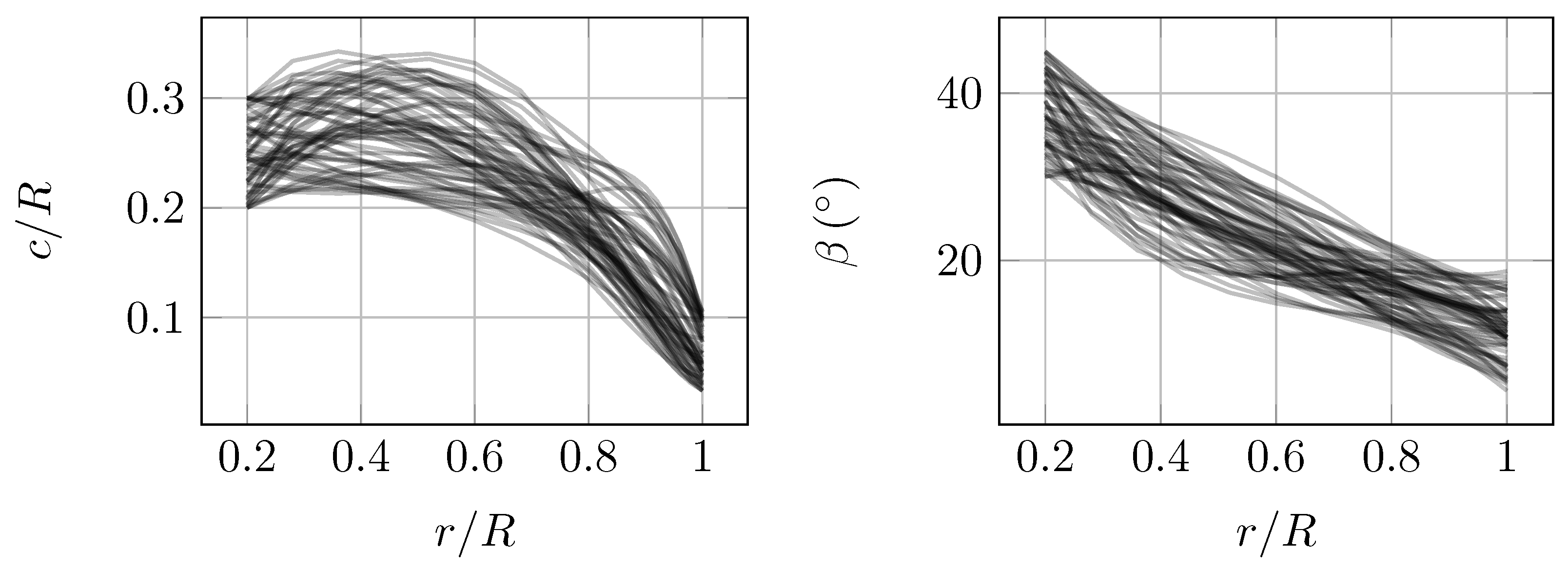
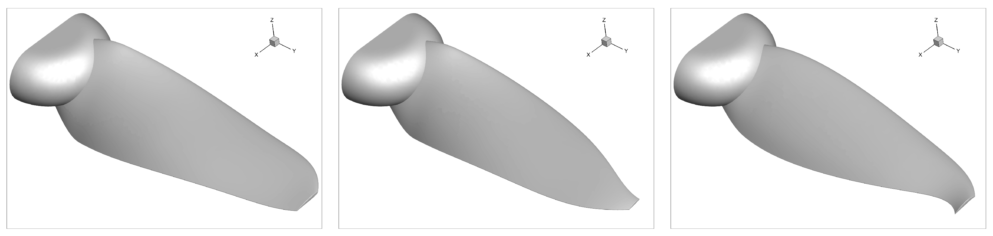
The resulting chord and twist distributions of the initial sample are visualized in Figure 8. It can be observed that a large search space was investigated in this study. The need for such variation in blade size (i.e., chords) and twist was dictated by the variable rotational speed, which has a large influence on the resulting forces. Three randomly selected samples from the initial sample are visualized in Figure 9.

The analysis of data obtained from a initial sample allowed us to verify the correctness of the computational model and optimization setup. The selection of design variables, including the definition of bounds, can be assessed with a global sensitivity study.

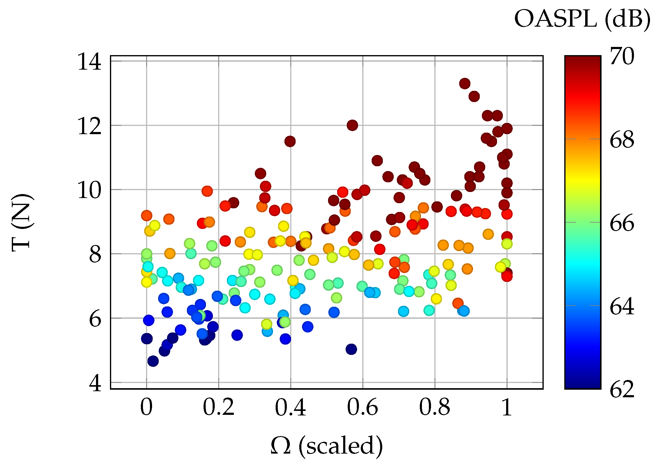
The initial sample consists of 200 points sampled in the design space of 20 variables. The current study is focused on finding the aeroacoustic optima which provide 8 $\mathrm{N}$ of thrust in hover. The analysis of Figure 10 ensures that a propeller providing sufficient thrust can be found for any rotational speed between 4200 and 5000 rpm (for convenience scaled to 0–1 in the plot). The thrust range for any rotational speed within bounds is around 6 $\mathrm{N}$ with a minimum of around $4.5$ $\mathrm{N}$ and the maximum exceeding 13 $\mathrm{N}$. A gentle trend of increasing OASPL with increasing rotational speed for a given thrust is noted.

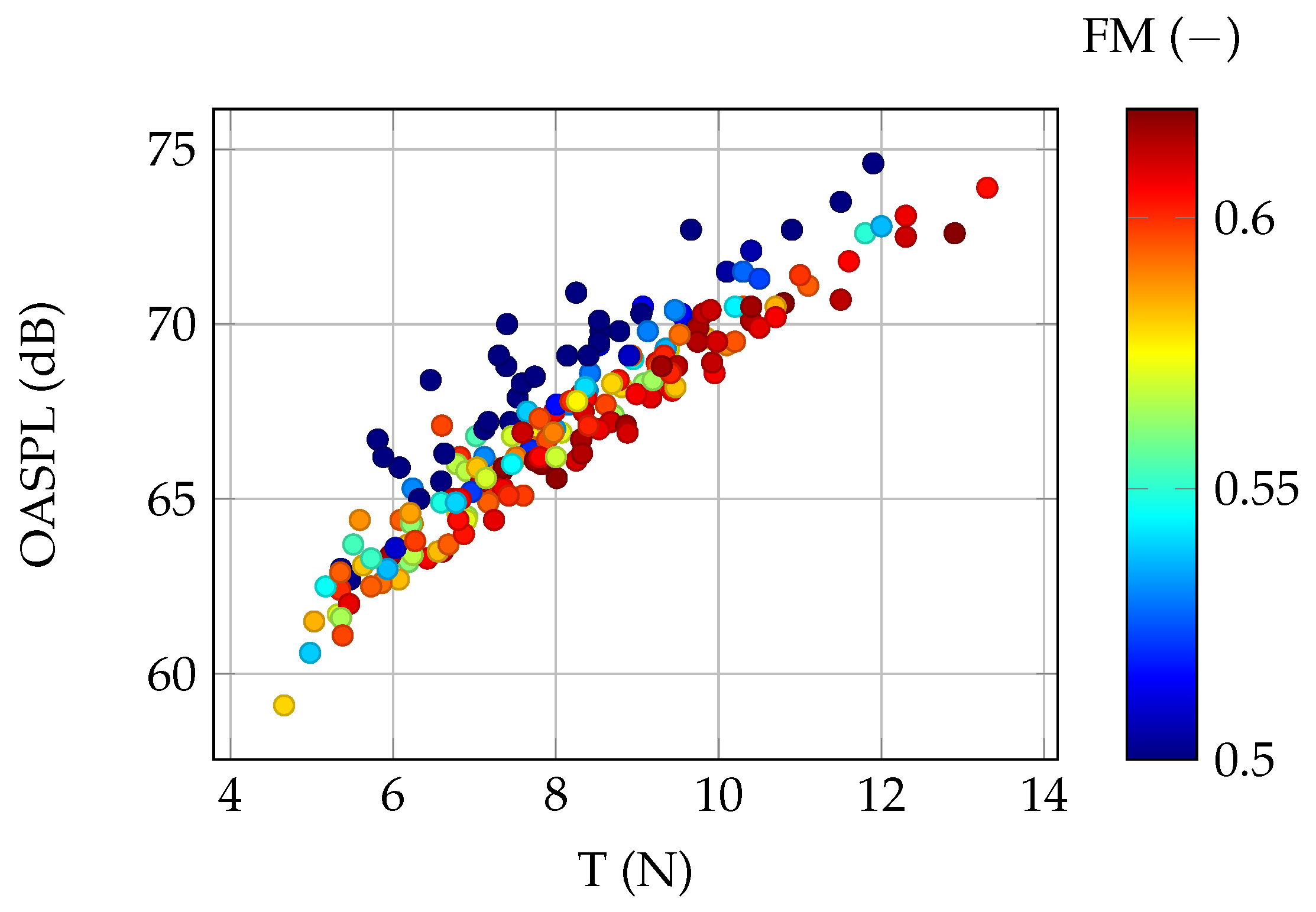
The linear correlation between thrust and the OASPL is presented in Figure 11. The correlation is even stronger if only individuals with a high FM are considered, i.e., the blue points are discarded. The task of concurrent OASPL minimization and FM maximization for a given thrust does not imply a clear trade-off—individuals with lower OASPL tend to have a higher FM. Consequently, the multi-objective optimization results are expected to form a relatively narrow Pareto front.

The analysis of global sensitivity of selected outputs was performed to reveal the importance of individual parameters. These results may be used in the infill-based iterative optimization process to build an efficient infill strategy. If unsatisfactory results are obtained, e.g., domination of one or few parameters, another optimization setup (parametric model) can be considered.

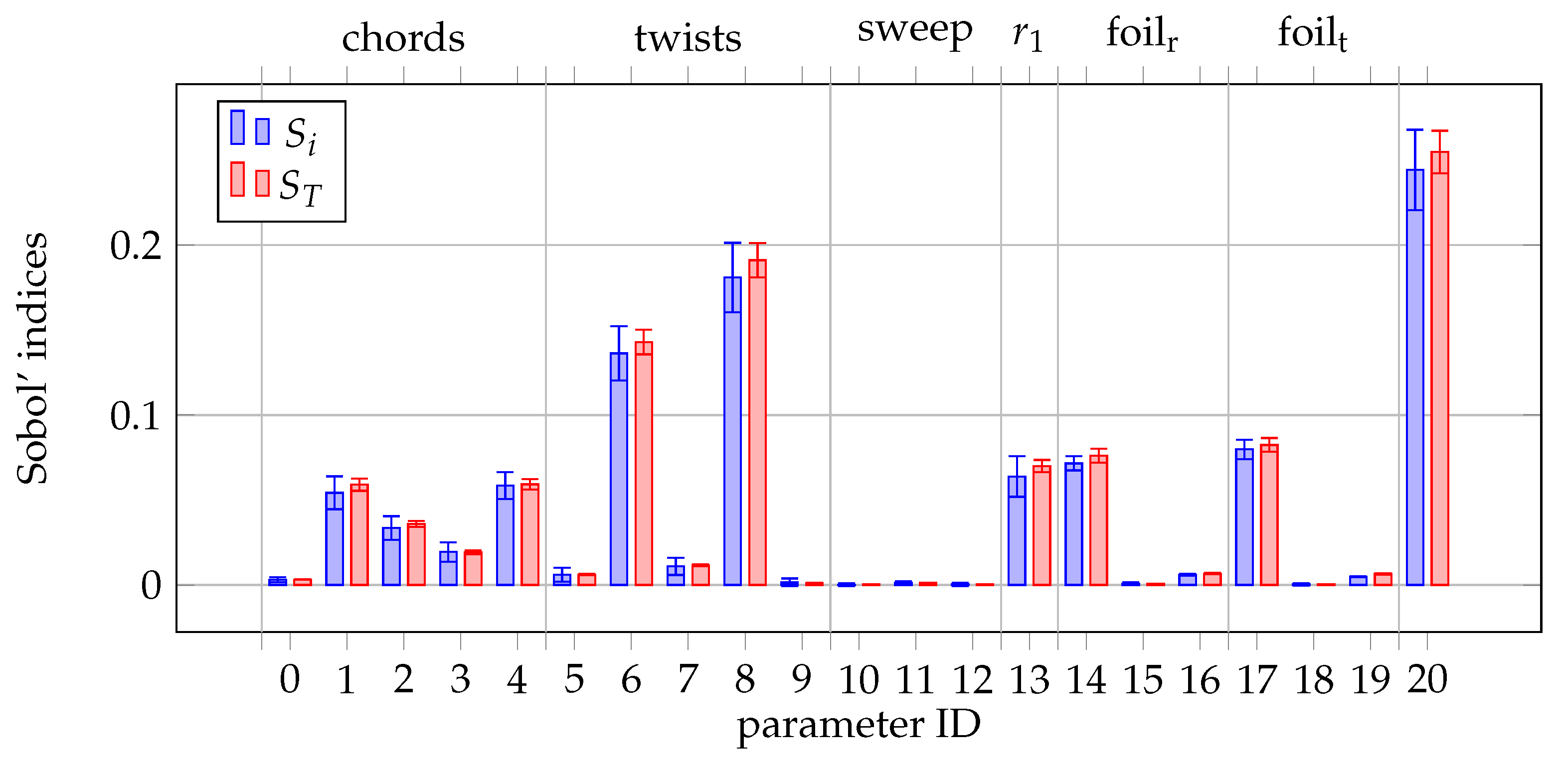
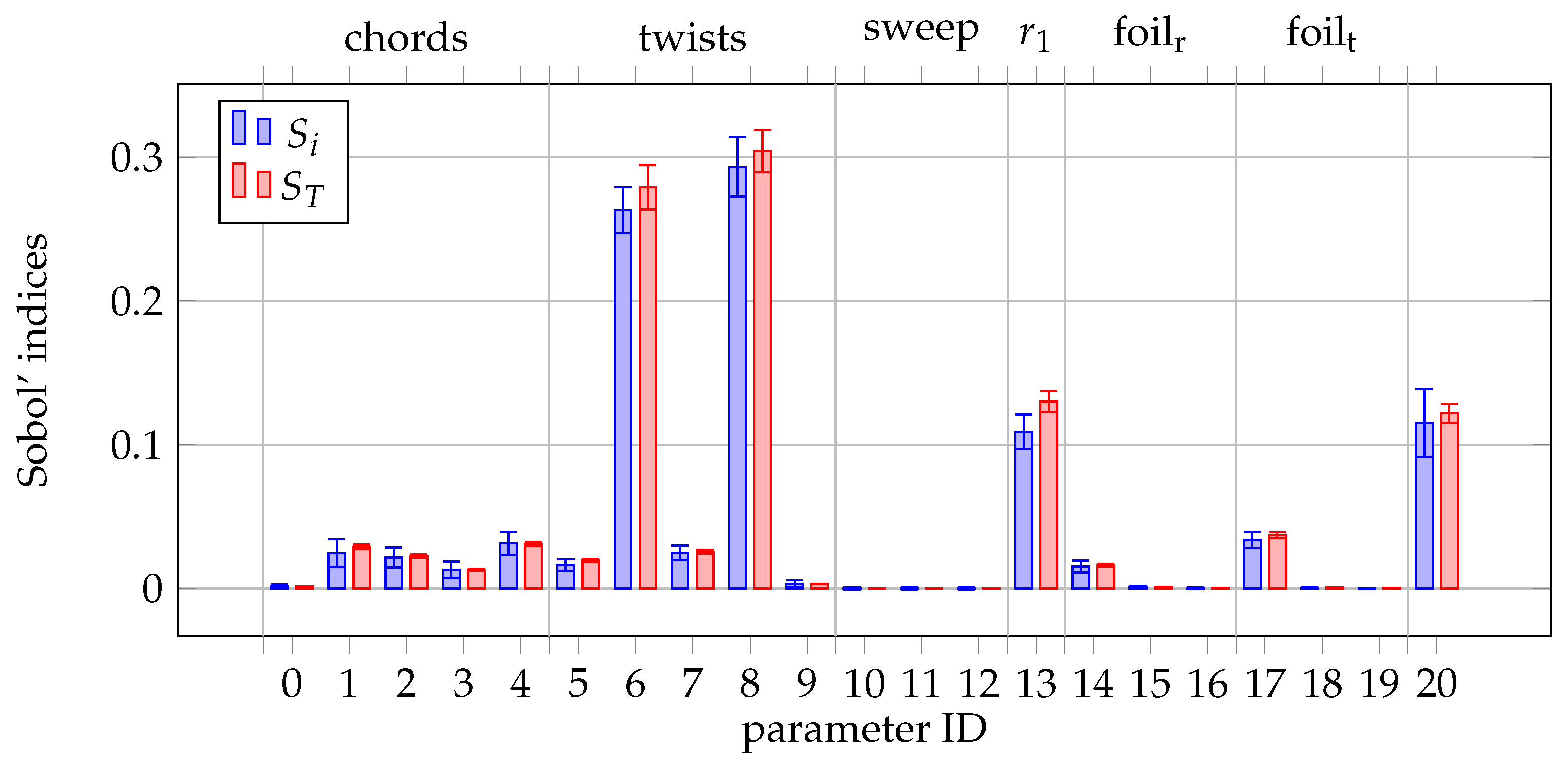
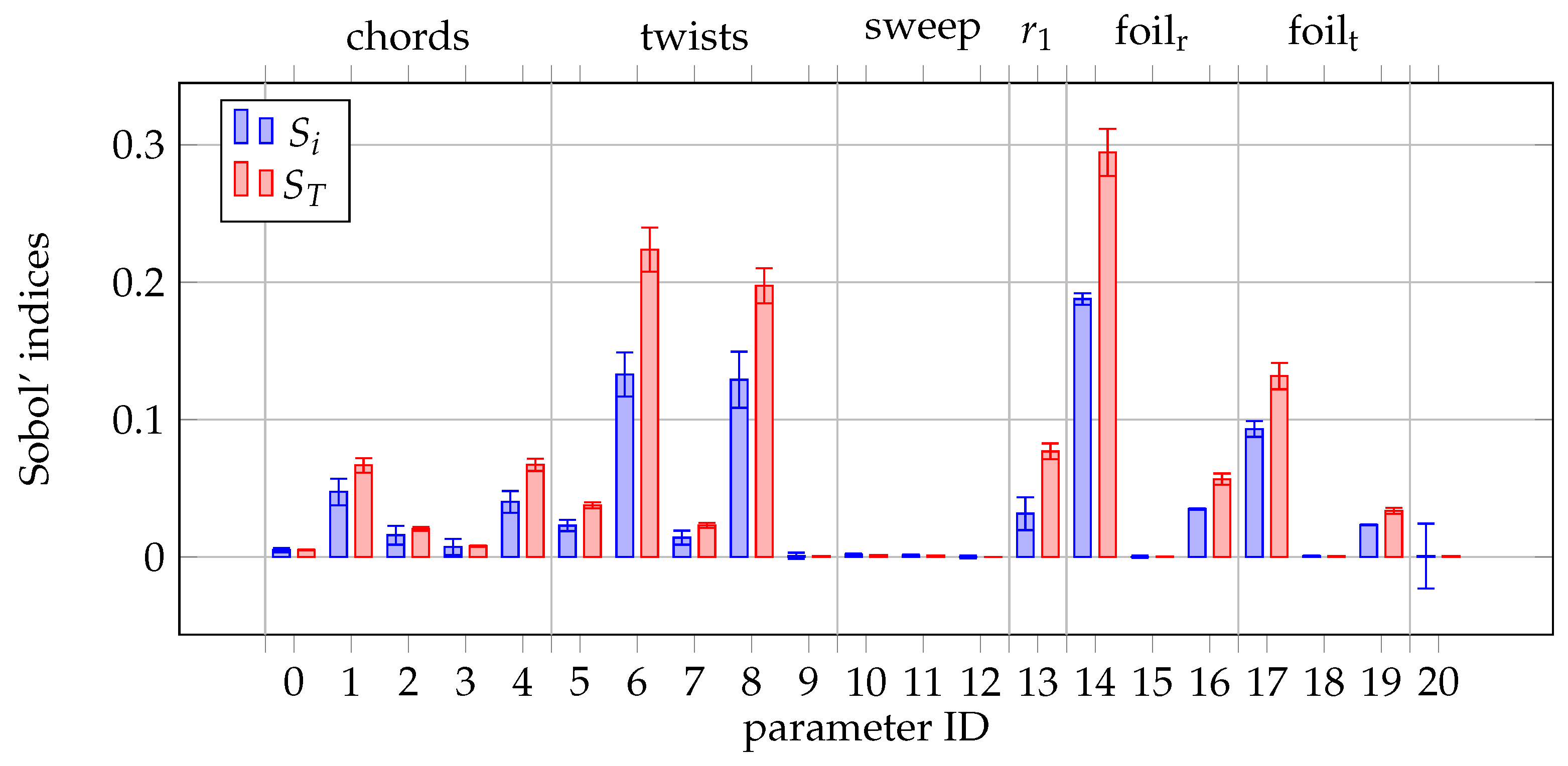
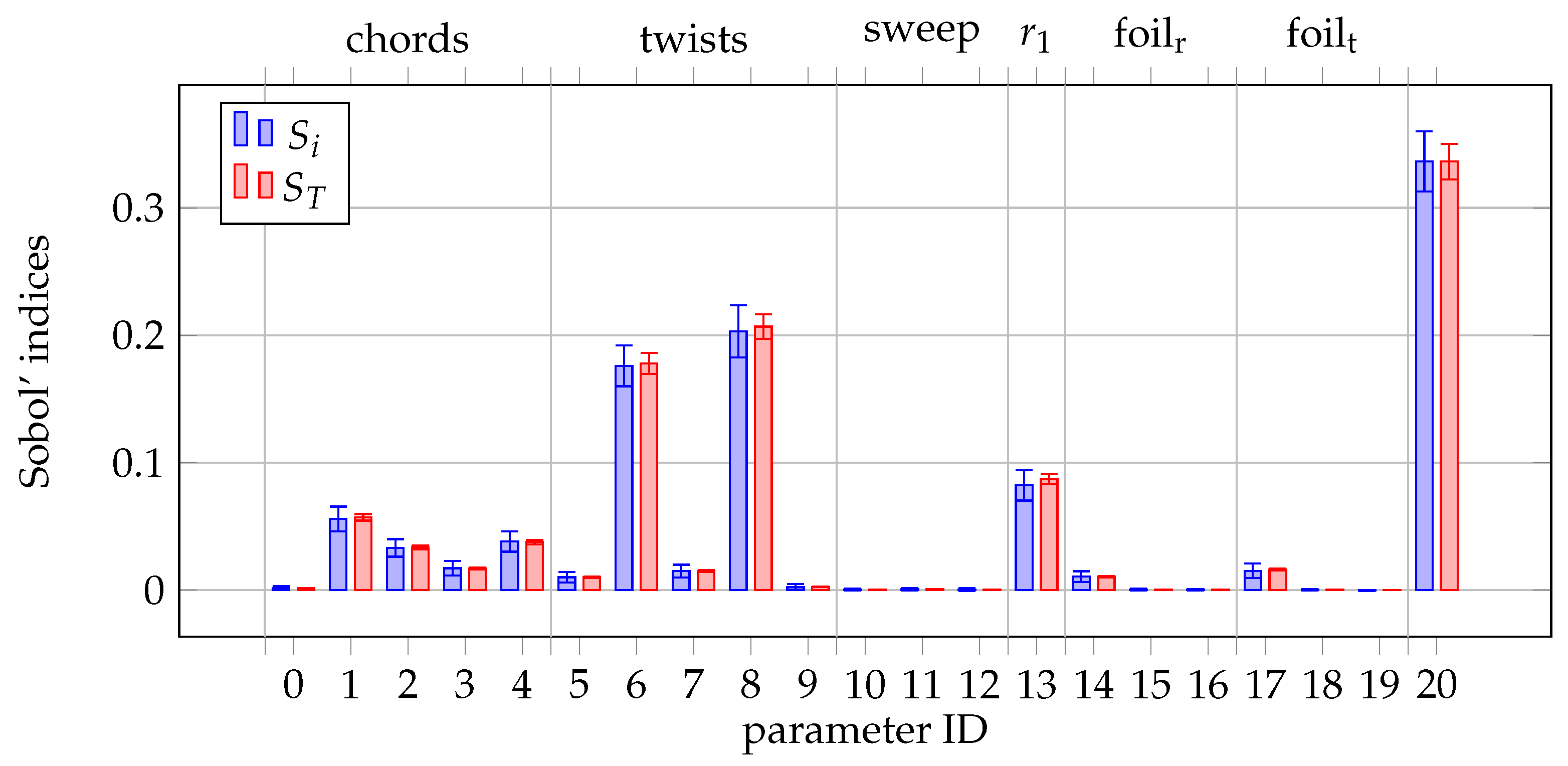
Figure 12, Figure 13, Figure 14 and Figure 15 present Sobol’ indices calculated with predictions of surrogate models for the following model outputs: thrust, torque, FM, and OASPL. Values of Sobol’ indices $S_i$ and $S_T$ were plotted for each design variable, according to the labeling defined in Table 2. Tags relating parameters IDs to their scope in the resulting geometry were added for clarity. Foil subscripts r and t stand for root and tip airfoils, respectively.

The sensitivity of thrust is the highest for rotational speed (parameter 20). Then, the highest importance was observed for knot positions defining twist (parameters 6 and 8), airfoil camber (parameters 14 and 17), and radial position of root airfoil (parameter 13). The remaining parameters defining the chord and twist distributions, as well as the sweep and remaining airfoil parameters, have a negligible effect on thrust. Similar trends are observed for torque sensitivity, with the two aforementioned twist parameters having the highest influence. The effect of sweep and maximum chord and camber position parameters is negligible, similar to thrust sensitivity. Sound pressure level is most sensitive to rotational speed and twist distribution. While both Sobol’ indices are very similar for all parameters of thrust, torque, and SPL sensitivities, some significant differences were noted in the case of FM model sensitivity. The differences in the values of $S_i$ and $S_T$ of the parameters defining airfoil camber and twist distributions, and to some extent of the remaining parameters, indicate interactions between them. This is an expected behavior, as these interactions are important in defining a blade geometry to ensure that the blade operates at the optimal effective angle of attack. In the physical sense, whether stall—which drastically decreases FM—occurs locally, is a combination of several factors, such as airfoil shape, local twist, and incoming flow. An important observation in the FM sensitivity is the lack of rotational speed influence. Consequently, it is expected that any rotational speed—within the defined bounds—allows for the achievement of the optimal FM.

Summarizing the global sensitivity analysis, the following conclusions regarding parametric definition can be drawn:

• Rotational speed dominates thrust and SPL output, but becomes negligible for the FM.
• Outputs from all presented models are more sensitive to twist than chord distributions. The bounds for twist might be unnecessarily wide or the bounds for chord parameters too narrow.
• The relative importance of parameter 8, defining the absolute twist at the tip, is dominating local twist perturbations (parameters 7 and 9) at the tip.
• Parameters 0, 9–12, 15, and 18, i.e., root chord, local tip twist, sweeps, and airfoil maximum camber position, are negligible in terms of all presented outputs.
• Apart from the FM model, the interactions between the parameters are very small.

5. Optimization

The multi-objective aeroacoustic optimization was performed with respect to 20 geometric parameters and rotational speed defined in $\mathbf{x}$. The target thrust of 8 $\mathrm{N}$ was defined as an inequality constraint (introducing tolerance) in order to improve optimization convergence. OASPL was calculated at the microphone located in the rotation plane, four diameters ($1.2$ $\mathrm{m}$) from the rotational axis (the same position as microphone 7 in the benchmark described in Section 3). The optimization problem is defined as follows:

$$\begin{array}{cc}\hfill \mathrm{minimize}:& \mathrm{OASPL},-\mathrm{FM}\hfill \\ \hfill \mathrm{with}\mathrm{respect}\mathrm{to}:& \mathbf{x}\hfill \\ \hfill \mathrm{subject}\mathrm{to}:& |T-8|-0.05\le 0\hfill \\ \hfill & \mathbf{l}\le \mathbf{x}\le \mathbf{u}\hfill \end{array}$$

(22)

The expected solution is in the form of a set of non-dominated points forming Pareto front.

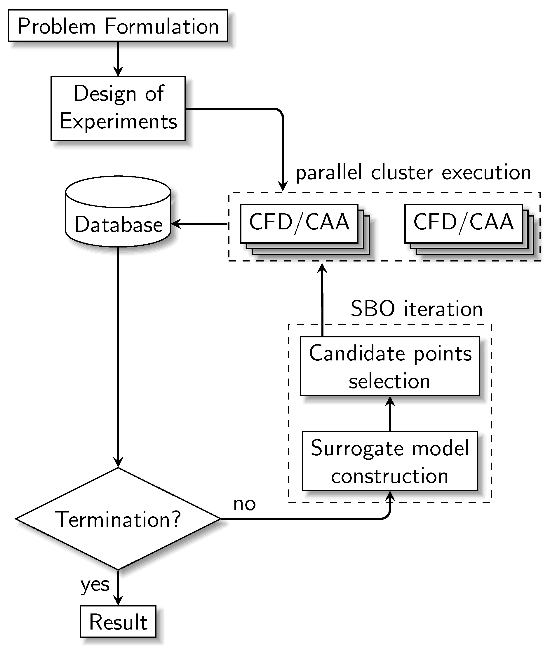
The SBO procedure defined in Section 2 and Figure 1 was followed to establish an aeroacoustic Pareto front. Three surrogate models were calculated for each interation: thrust, FM and OASPL, which were used to provide cheap approximations for the objectives and constraint. The Scipy [35] differential evolution (DE) algorithm was used to search for infill points. DE is a stochastic optimization method, used for finding the global optimum of a multivariate function with constraint handling capabilities. The following infill criteria were used at each iteration to obtain a set of infill points and to take advantage of parallel case execution:

• minimization of OASPL,
• minimization of −FM,
• maximization of EI of OASPL,
• maximization of EI of −FM, and
• minimization of a weighted OASPL and −FM (used to establish the Pareto set).

Additional infill points were achieved by searching in limited rotational speed regimes, i.e., the bounds for the search were tightened in the consecutive ranges: (0–0.25), (0.25–0.5), (0.5–0.75), and (0.75–1) of the original 0–1 range of $\omega$.

5.1. Surrogate Model Prediction

Surrogate models of thrust, and OASPL were assessed with MSE and MAE performance metrics. An approach similar to the one described in [28] was used: for each surrogate model, a set of 30 evaluations of MSE and MAE were performed, based on random selection of test samples. Average values of error metrics and standard deviations for each model were summarized in

Table 3. Sumary of MSE and MAE for surrogate models used in the optimization.

Model	MSE (std)	MAE (std)
thrust (N)	0.0158 (0.0205)	0.2575 (0.0818)
FM (−)	$1.13\times {10}^{-4}$ ($6.31\times {10}^{-5}$)	0.0254 (0.0073)
OASPL (dB)	0.0344 (0.0114)	0.4774 (0.0716)

. The quality of prediction was deemed sufficient for optimization.

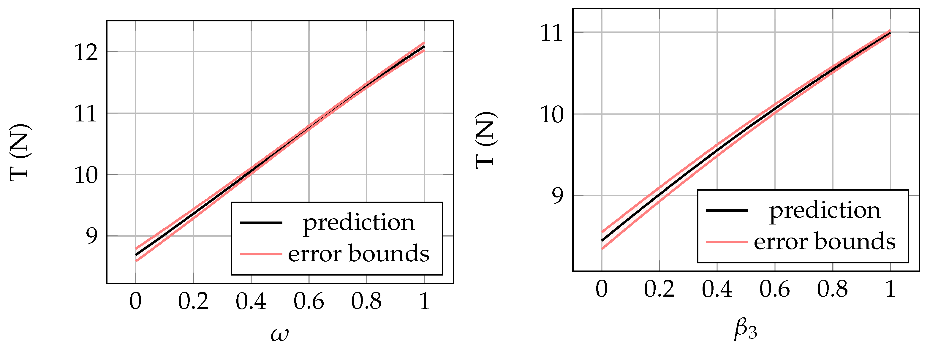
High prediction accuracy of surrogate models built from a relatively sparse sample in a multi-dimensional space was attributed to the relatively simple model output landscape. Figure 16 presents predictions along with the prediction error of the two most active variables in the model—$\omega$ and ${\beta }_3$. The values of remaining parameters are fixed to the mean value (between the lower and upper bounds). The total thrust difference within the rotational speed exceeds 3 $\mathrm{N}$, which is expected from the analysis of the initial sample in Figure 10. Changing ${\beta }_3$ from the minimum to the maximum results in a thrust change of approximately $2.5$ $\mathrm{N}$. These predictions are consistent with the global sensitivity analysis presented in the previous section.

5.2. Optimization Flow

The iterative optimization procedure defined in the previous section was run for three infill iterations. The infill points from the first infill were selected from a region with a relatively small surrogate model confidence, which resulted in a significant prediction error. After the first three infills, the congestion of infill points in a limited area caused problems in fitting the surrogate model. The subsequent iterations used limited infill points to address this issue. As the data sample was filled with additional data from infill points, the surrogate prediction of thrust improved. The problem of a slightly underestimated thrust (typically by up to $0.3$ $\mathrm{N}$) remained throughout the whole process. It was observed that the thrust error was very low (less than $0.02$ $\mathrm{N}$) if the surrogate model is built with data for the geometry of interest, i.e., the surrogate model predicts changes in thrust for a given geometry very well. Hence, the results obtained from the CFD verification of infill points were valuable in setting the target $\omega$ to achieve the desired thrust. The determination of the final result (Pareto front) was based on the CFD model, i.e., the desired thrust of 8 $\mathrm{N}$ was verified.

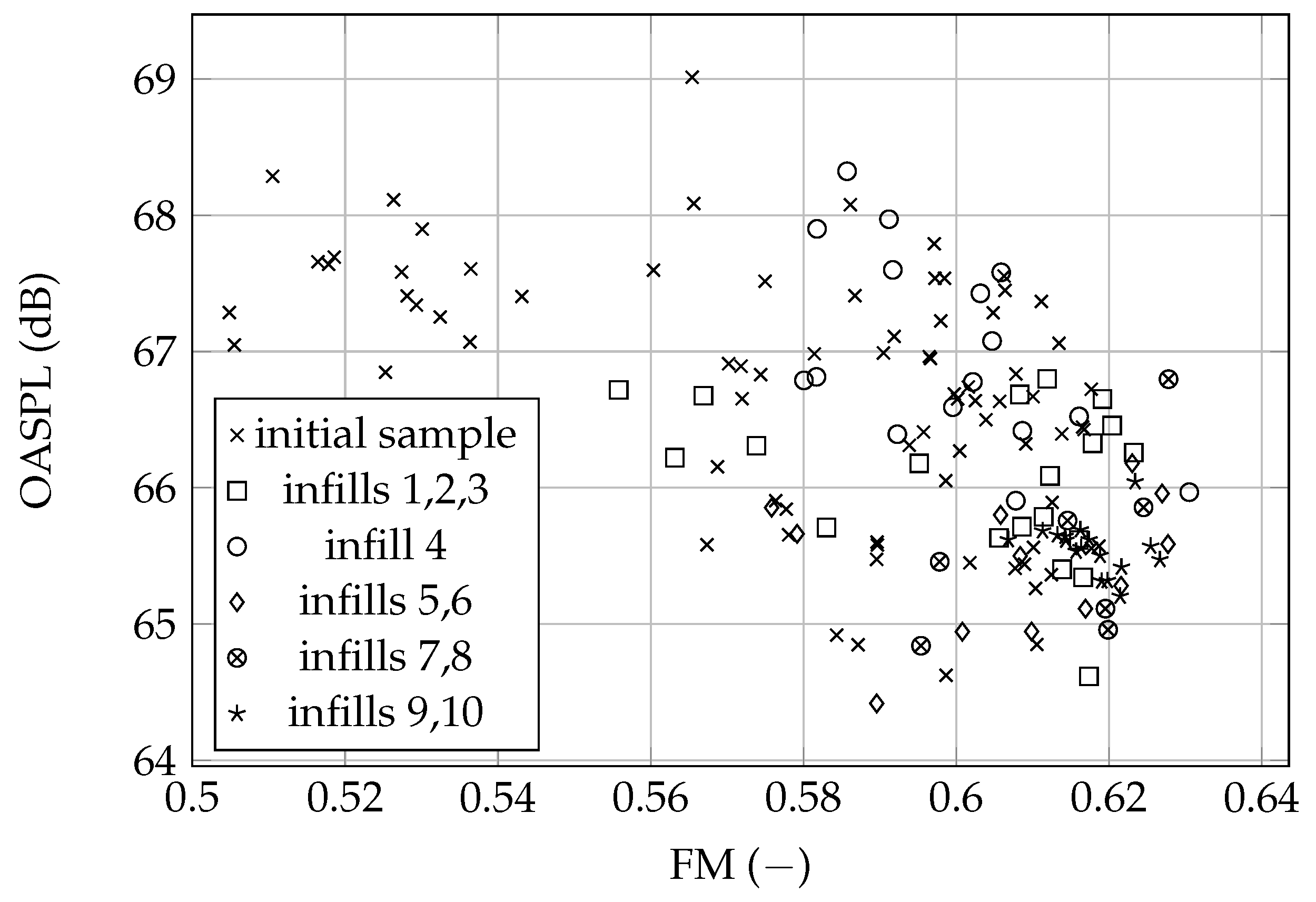
The optimization process was terminated after 12 iterations, as no new point was added to the Pareto front for two consecutive iterations. The lack of improvement was attributed to the surrogate prediction error and a very tight margin for potential improvement. The aeroacoustic Pareto front, presented in Figure 17, turned out to be very narrow—the difference between OASPL-optimal and FM-optimal designs was approximately $1.5$ dB and just above 0.01 FM counts. The point minimizing OASPL with a FM approximately 0.59, theoretically being Pareto optimal, extends the FM range. However, it offers very little improvement in OASPL compared to the second-best. Consequently, it is unlikely to be considered as a practical solution.

In a summary, the observed optimization flow can be divided into three stages:

• The first three infill iterations—high prediction error of the infill points resulted in designs providing insufficient thrust. This stage was important in improving the surrogate model prediction in the promising areas.
• Infill iterations 4–8—reasonable surrogate model prediction allowed to find a number of Pareto optimal solutions.
• Infill iterations 9–12—many infill points in promising areas of the search space. The surrogate model prediction was relatively good, however, no further optimal solutions were found.

The whole optimization process, including both initial sample and infill iterations took approximately 50–60 thousand CPU hours. Both initial sample and infill interations took advantage of parallel case execution, which allowed us to complete all computations within a week on High-Performace Computing (HPC) cluster. Consequently, SBO applied to RANS-based global propeller design was feasible from a computational point of view.

5.3. Results Analysis

The analysis of optimization results in the current work is focused on the qualitative aspects of the obtained results, rather than on the selection of particular design(s). For this purpose, two blade designs obtained from the Pareto set are compared: the FM and OASPL optima. A CFD verification confirmed the accuracy of predictions provided by surrogate models for both cases.

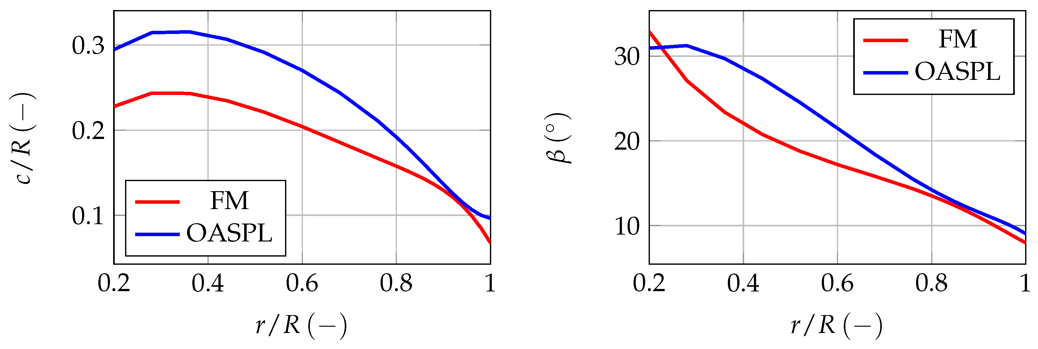
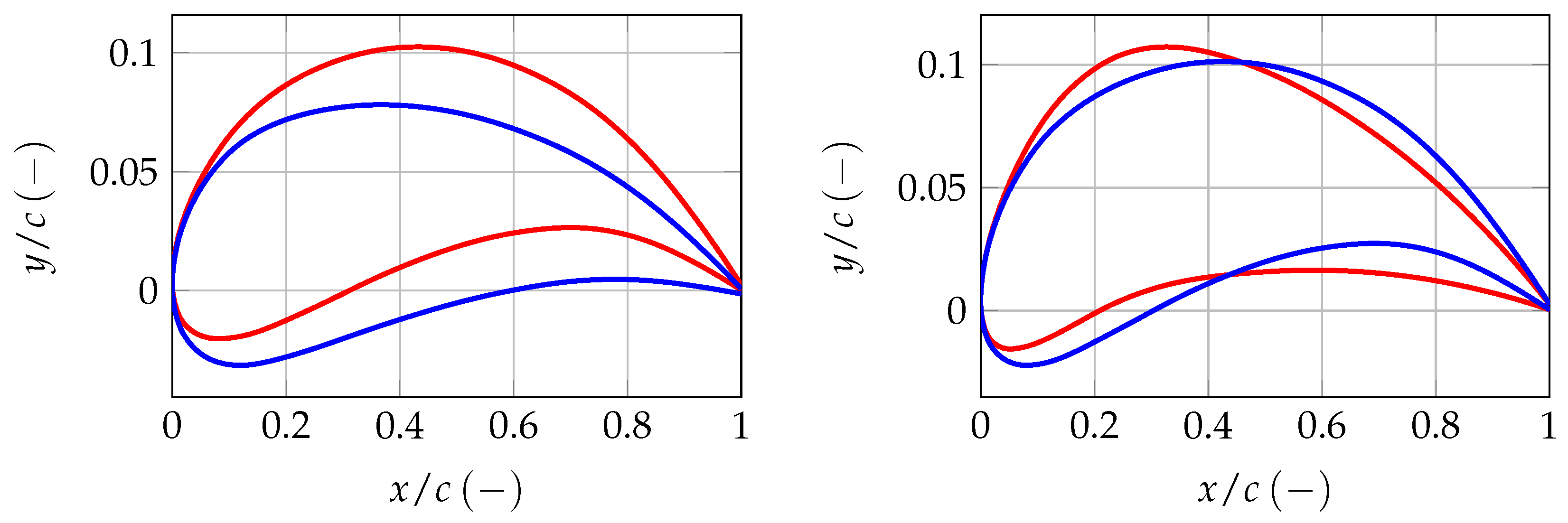
Figure 18 presents distributions of chord and twist along the radius for the FM- and OASPL-optimal propellers. Major differences can be observed: the FM optimum has a higher aspect ratio and lower twist, especially in the inboard part of the blade. The design rpm, i.e., rotational speed required to achieve the target thrust, is 4740 and 4250 for the FM and OASPL optima, respectively. Airfoils used to define the stacking of both propellers are presented in Figure 19. The camber of the root airfoil is significantly higher in the FM-optimal design, which explains the difference in twist. The tip airfoils have a similar camber magnitude, which is expected, as the twist distribution is similar near the tip.

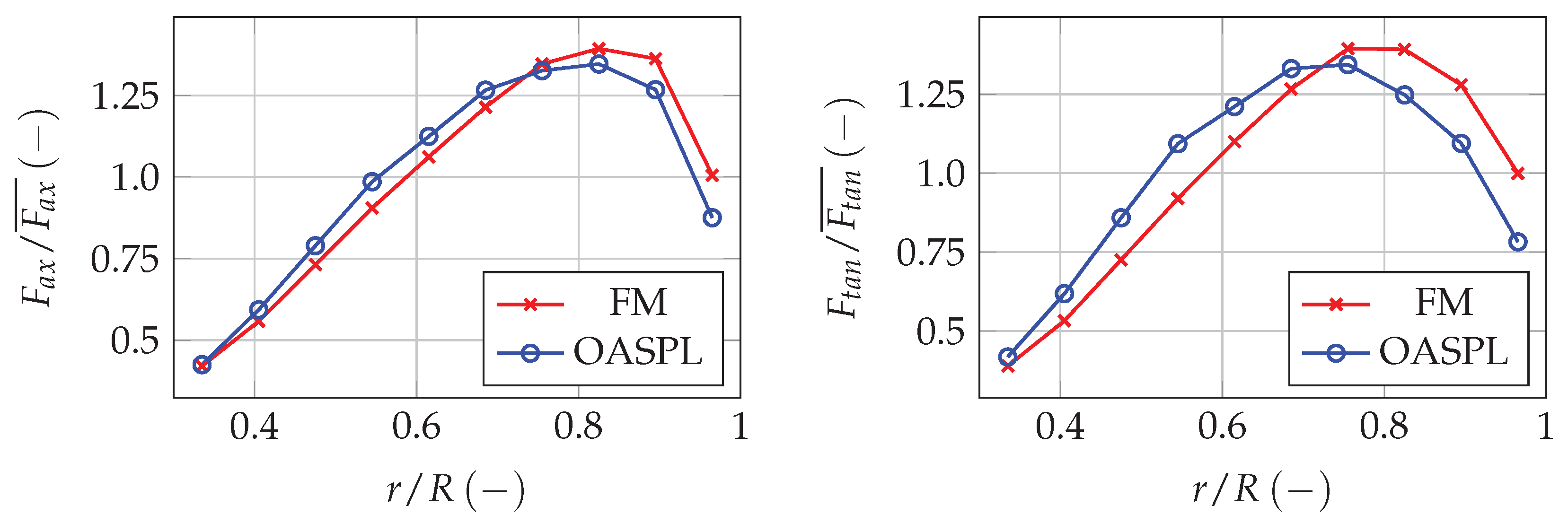
The axial and tangential force distributions along the radius, computed from the CFD model, are presented in Figure 20 for FM and OASPL optima. It can be observed that the OASPL optimum has the loading shifted towards the rotation axis, compared to the FM optimum. Similarly, peak values are higher for the FM optimum. These trends are expected, as noise reduction is achieved by lowering peak pressure, which is the highest near the tip. It should be noted that the differences in the distributions of dominating axial force are not very large. This is a result of the limitations of the parametric model, which prevented the loading from being shifted further towards the root of the blade.

To conclude the optimization results, it should be noted that all expected trends regarding noise-minimizing propeller design were reproduced. Apart from that, local shape features—such as airfoils—were selected by the optimizer, based on the blade geometry-resolved CFD. Consequently, the results are expected to be of high accuracy. The methodology can be used with custom parametric models, including geometry features which require blade-resolved CFD, such as winglets.

6. Conclusions

A comprehensive study of computational modeling of a propeller blade was presented. The optimization context of the study constrained the computational cost of the CFD and CAA models. As a result, the blade-resolved steady RANS model was used, with tonal noise calculation based on the F1A formulation of FWH aeroacoustic analogy applied to a blade surface. The methodology was validated against a literature benchmark. The resulting balance between computational cost and model fidelity and robustness allows to perform a global surrogate-based optimization. A global sensitivity study was performed using Sobol’ indices. The results show the relative importance of individual design variables (geometric parameters and rotational speed) on force outputs and efficiency metrics. Consequently, an optimization strategy was devised, to establish the Pareto front of aeroacoustic optimization. The selection of the final design still questions the objective function specification (e.g., desired microphone(s) location for noise minimization, relative importance of aerodynamic and acoustic performance, etc.).

The key findings of the work are:

• Global multidisciplinary aeroacoustic optimization of a propeller blade using RANS equations and the FWH analogy can be performed at a reasonable computational cost using robust blade-resolved methods. Assuming parallelization capabilities and the nature of surrogate-based optimization, the associated total computational time is relatively small. Further computational time reductions can be achived by reduction of parametric model dimensionality.
• The parametric model of the blade geometry is the most sensitive to the twist distribution, which affects the local effective angle of attack. The airfoil camber and chord distributions are less significant. Sweep has a negligible influence on the performance metrics used in the current study.
• An implicit definition of geometric variables in the parametric model (i.e., the definitions of chord and sweep at the tip) can result in misleading sensitivity study results. In this study, the tip twist parameter (${\beta }_4$) has a relatively small effect on thrust, the FM, and torque as a result of its implicit definition.
• The spline-based approach yields a parametric model which results in virtually no parameter interactions for thrust, torque, and SPL. Only in the case of FM do the interactions between parameters become significant.
• SBO allows for performing a range of different optimizations, basing on the starting data sample. The objective function can be modified during the optimization process without loss of data and computational effort. Examples are: a switch between raw and A-weighted OASPL, or a redefinition of noise metrics from one to another microphone.

The limitations of the current work, which will be addressed in future work, are:

• The CAA model used in the current work calculates only the tonal part of noise. When propellers of a smaller scale are investigated, where the broadband part of noise becomes important, or a when a different objective function is addressed, e.g., focused on mitigation of high-frequency noise, the broadband noise should be included in the model.
• System-level noise resulting from aerodynamic interactions between propellers and vehicle body should be investigated to fully address the problem of noise emission.