A Multivariable Method for Calculating Failure Probability of Aeroengine Rotor Disk

Abstract

The probabilistic damage tolerance analysis of aeroengine rotor disks is essential for determining if the disk is safe. To calculate the probability of failure, the numerical integration method is efficient if the integral formula of the probability density function is known. However, obtaining an accurate integral formula for aeroengine disks is generally complicated due to their complex failure mechanism. This article proposes a multivariable numerical integral method for calculating the probability of failure. Three random variables (initial defect length a, life scatter factor S, and stress scatter factor B) are considered. A compressor disk model is evaluated. The convergence, efficiency, and accuracy of the proposed method are compared with the Monte Carlo simulation and importance sampling method. The results show that the integral-based method is 100 times more efficient under the same convergence and accuracy conditions.

1. Introduction

In recent years, probabilistic damage tolerance analysis (PDTA) has proven its potential in the life management [1] of aeroengine rotor disks in civil and military areas. This probabilistic method considers random events in both the manufacturing and utilization phases, such as undetectable material processing anomalies, random loads, crack growth rate, inspection schedules, and the probability of detection, to enhance the safety of rotor disks [2,3]. Compared with the conventional life management methodology (also called the safe life method), PDTA promotes rotor integrity against anomalous material aspects under the required manufacturing conditions. Therefore, such a methodology has been requested by the airworthiness authorities of major aviation industry countries, such as the Federal Aviation Administration [4], the European Union Aviation Safety Agency [5], and the Civil Aviation Administration of China [6]. In addition, the need for the application of PDTA to fatigue life prediction of gas turbine engine components is being increasingly recognised by the U.S. Military [7].

Over the past two decades, under the direction of the Federal Aviation Administration, the Southwest Research Institute, in conjunction with four major aircraft engine manufacturers (General Electric, Honeywell, Pratt & Whitney, and Rolls-Royce), has developed and enhanced the PDTA program DARWIN to address inherent material anomalies in titanium alloys and nickel-based superalloys [8], including manufacturing- and maintenance-induced anomalies [9,10,11,12,13]. DARWIN is an approved tool for compliance with Advisory Circular 33.70-1 [14,15] (titanium hard alpha) and Advisory Circular 33.70-2 [4] (hole features).

The general procedure of PDTA for inherent material anomalies, as depicted in Figure 1, is divided into three parts: the inputs, the outputs, and the analysis process [16]. The inputs include the initial defect/crack size distribution, finite element stress, material properties, etc. These inputs are obtained from industrial or experimental data accumulated by aeroengine companies. Before the probability of failure (POF) calculation, the stress analysis, zone definition, and crack growth analysis should be performed. Then, both zone and disk POFs are calculated. The zone POF determines the most dangerous region for further risk analyses. Once the disk POF exceeds the design target risk value, the disk design needs to be improved.

The process mentioned above has been proven to be a reasonable method and has been successfully accepted by airworthiness authorities. However, the probability calculation usually incurs a cost problem because of the large number of Monte Carlo simulation (MCS) samples [17,18,19]. For this process, the time cost is determined by the efficiency of the fatigue crack growth calculation of each MCS sample and the MCS sample size. The high-efficient fatigue crack growth models [20,21,22] improve the calculation efficiency of MCS and other probabilistic calculation methods, e.g., the importance sampling and numerical integration (NI) method. Nevertheless, the enormous MCS sample size is the critical reason for the calculation cost problem because the aeroengine rotor disk’s design target risk value is low, usually less than 10⁻⁷. Hence, developing a practical probability calculation algorithm to solve the MCS sample size problem is significant for improving the analysis efficiency and decreasing costs. The methods studied and proposed in recent decades can be summarised in the following sections.

(1) Improved MCS method

Improving MCS is a general method used to improve calculation efficiency. In PDTA, the disk is separated into zones for POF calculation. The calculation mechanism of zone condition failure probability is $P_{\mathrm{f}}{=N}_{\mathrm{fail}}{ / N}_{\mathrm{zone}}$, where $N_{\mathrm{zone}}$ is the number of MCS samples per zone. The size of $N_{\mathrm{zone}}$ is always 10⁴–10⁶ or greater to guarantee high accuracy. Therefore, the total number of samples $N_{\mathrm{total}}{=N}_{\mathrm{zone}}{ \times n}_{\mathrm{zone}}$ is always enormous for a real disk case, where $N_{\mathrm{total}}$ depends on the number of samples per zone ($N_{\mathrm{zone}}$) and the number of zones ($n_{\mathrm{zone}}$). Consequently, the computational efficiency problem is transformed to reduce $N_{\mathrm{zone}}$ and $n_{\mathrm{zone}}$.

Methods dedicated to reducing $N_{\mathrm{zone}}$ include the importance sampling method [23] and the adaptive optimal sampling technique [24]. The two methods differ in their approaches to reducing the sample size. The importance sampling method generates only those samples that will result in a lifetime smaller than the target service life by defining the critical initial defect size $d^{*}$. The MCS sample sizes are decreased without increasing the variance with this technique [25]. The adaptive optimal sampling technique is an algorithm that adaptively allocates samples to member failure modes based on initial estimates of the individual member failure probabilities [24].

Another approach is to reduce the number of zones $n_{\mathrm{zone}}$ by adopting the zone refinement technique [25] and joint probability density functions [26]. In the zone refinement technique, each zone’s risk contribution is reduced to less than a specific limit value via refining the zones with a high-risk contribution [25]. The joint probability density function is obtained from an adaptive refinement of the element mesh where elements are subdivided based on their contribution to the component risk [26]. Additionally, the adaptive optimal sampling technique can be combined with the zone refinement technique to reduce the sample size [27].

(2) Numerical integration (NI) method

Unlike the methods used to reduce the number of MCS samples, the NI method calculates the POF by integrating the joint probability density function. In the PDTA of aircraft structures, the mixed techniques of MCS and probability integration algorithms can balance the speed and accuracy of POF calculation [28]. However, the explicit formula of the density function of POF at current N cycles is often complicated to solve, especially under the rotor disk’s complex failure mechanism. In 2017, Yang introduced a fast NI algorithm based on probability density evolution, which established a relationship between the initial probability distribution (N = 0) and the actual distribution after N flight cycles. Hence, the POF is determined directly through the initial anomaly distribution [29]. The results show that the analysis cost is vastly decreased compared to the traditional MCS method.

However, the fast NI algorithm only takes the single random variable of the initial crack size into consideration. This algorithm has not dealt with the multiple random variables of practical PDTA. The analysis of multiple random variables is essential in PDTA since the POF is closely related to the uncertainty of the initial crack size, load, and material [30]. Assuming that these variables obey the corresponding probability statistical distribution, the specific mathematical demonstration and the implementation algorithm of the fast NI algorithm are unknown. Moreover, the previous research has not treated of NI method’s convergence in much detail. Commonly, with the NI method’s integral step size decreased, the calculation results converge, but the time cost increases. Therefore, it would be valuable to investigate whether the NI method’s high accuracy and efficiency could be maintained considering multiple random variables under the condition of convergence.

This study extends the fast NI method from single-variable to multivariable to meet the requirements that originate in the actual PDTA. Considering the random initial defect length a, stress scatter factor B, and life scatter factor S, the multiple integral and the specific analysis process are established with multivariable based on the probability density evolution theory. Furthermore, the convergence, accuracy, and efficiency are compared among the proposed multivariable NI method, MCS, and importance sampling method with the multivariable consideration using an actual compressor disk model. The time costs of the NI method and MCS using different numbers of random variables are also analysed. This research can provide an additional reference for general designers in assessing disk POF.

This paper is divided into five sections. Section 2 describes the mechanism of probability density evolution theory and the multivariable NI method. An evaluation of the centrifugal compressor disk model is presented in Section 3. Section 4 characterises the convergence results and compares the different cases employed in the proposed method, MCS, and importance sampling method. Finally, Section 5 summarises the principal conclusions.

2. Multivariable Numerical Integration Method of Probabilistic Damage Tolerance Analysis

This section first describes the three random variables considered in the practical PDTA process. Then, the mechanism of establishing the multivariable integration model is explained. Finally, the realisation process of the multivariable NI method is presented in detail. Figure 2 compares the proposed method in this work with the MCS process and the single-variable NI method, which shows the probabilistic calculation method’s development.

2.1. Multiple Random Variables Considered in the PDTA

In general, the PDTA considers five random variables, including the size and frequency of the crack-inducing anomaly, the stress scatter factor, the life scatter factor, the time of non-destructive inspection during the service life, and the POD for each non-destructive inspection type [31,32]. However, the essential purpose of PDTA is to evaluate whether the failure risk satisfies the disk’s designed target risk (DTR) condition. The non-destructive inspection reduces the failure risk during the service life when the DTR is not satisfied or continues reducing the failure risk. Additionally, the time of the non-destructive inspection is a designed time rather than a statistical variable. Consequently, this paper considers the design evaluation stage, three variables, a, B, and S, are investigated. In analysing these three variables by the NI method, the key objective is to convert the integral probability region to the initial variable space, and the variable space needs to satisfy the conservation of the probability condition.

Therefore, in this study, the size and frequency of the crack-inducing anomaly, the life scatter factor, and the stress scatter factor are taken as the random variables. These variables are presented in detail in this section.

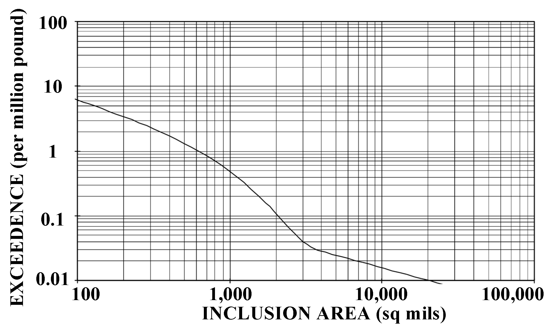
2.1.1. Initial Defect Size of the Material

In this article, the oversize initial material defect is considered to be the leading cause of the aeroengine rotor disk fracture. The initial defects of the materials mentioned here usually refer to inclusions that arise during the metal melting process, such as hard-$\alpha$ inclusions. The following part of this article shall not distinguish between cracks, defects, anomalies, and inclusions.

Although the probability of hard-$\alpha$ inclusions occurring in the material is low, usually 10⁻⁶, this condition is challenging to detect utilising non-destructive inspection due to the slight difference in density between the hard-$\alpha$ inclusions and the matrix. Moreover, if such defects with high hardness are contained in the structure, cracks will quickly develop under alternating load during use. These cracks may lead to a fracture of the structure, potentially causing a severe accident.

At the end of the 20th century, the American Aerospace Industry Association and the Rotor Integrity Subcommittee jointly developed a method to determine the initial defect distribution based on a large number of practical industrial experiences [33]. The defect distribution information is the occurrence frequency of an initial defect of a specific size in a unit material mass (or volume). Figure 3 shows the defect size distribution curve, representing the number of initial defects greater than a specific length per million pounds of material. The curve is only a general description of the initial defects. For probability calculations, the initial defect distribution data must be converted into a cumulative distribution function to perform MCS or NI calculations.

In general, the structural safety life includes the crack initiation life and crack stability extension life. However, if undetected defective titanium alloys have been placed into use after the forging process, inevitable initial cracks have already started around the defects. Thus, to simplify the risk analysis process, the cracks’ initiation life is generally assumed to be zero, and the initial crack length is considered the same as the initial defect length. In addition, for the sake of conservative results of life evaluation, the defects are assumed to be flaky circular cracks and treated in the infinite plate subjected to a uniform stress perpendicular.

2.1.2. Life Scatter Factor

The fatigue crack growth model is generally described as a function of the growth rate, stress intensity factor $\mathrm{\Delta }K$, and stress ratio R, as shown in the following:

$$\frac{\mathrm{d}a}{\mathrm{d}N}=\psi (\mathrm{\Delta }K,R),$$

(1)

where a is the size of the crack, N is the number of flight cycles experienced during engine service, K is the stress intensity factor at the crack tip, which is solved by the finite element method, Newman shape factor method [34], or weight function method [35], and the stress ratio R = 0 considering the engine take-off and landing cycle.

The parameters in the fatigue crack growth model are obtained by curve fitting the experimental data [36]. Due to the dispersion of the experimental data, the fitting results tend to be uncertain. To characterise the uncertainty of crack growth life, the life scatter factor of S is classified as the uncertainty of the crack growth model and added to Equation (2)

$$\frac{\mathrm{d}a}{\mathrm{d}N}=S\cdot \psi (\mathrm{\Delta }K,R),$$

(2)

where S can be obtained from different crack growth models, such as the Paris law [37], Walker law, Forman law, or NASGRO law. For example, when applying the Paris law, see Equation (3)

$$\frac{\mathrm{d}a}{\mathrm{d}N}=S\cdot C{(\mathrm{\Delta }K)}^n.$$

(3)

2.1.3. Stress Scatter Factor

The stress scatter factor B represents the uncertainty of the alternating load that the engine disk experiences. This uncertainty mainly affects the value of the stress intensity factor K. For example, the Newman shape factor method for calculating the stress intensity factor is shown in Equation (4)

$$K=Q\cdot \sigma \sqrt{\pi a},$$

(4)

where Q is the crack’s shape factor, characterising the structure’s geometric modification. $\sigma$ is the structure’s equivalent stress.

The stress value of $\sigma$ is usually calculated using commercial finite element software to simulate the engine structure. The stress scatter factor B is introduced into the probability calculation in Equation (4) to consider the stress’s uncertainty. Similarly, B follows a particular probability distribution so that the stress value has a degree of dispersion.

$$K=Q\cdot B\cdot \sigma \sqrt{\pi a}.$$

(5)

The scatter factors of B and S introduced above are generally considered to satisfy log-normal distributions, whose probability density function is as follows. The mean and variance can be obtained by evaluating the results of fitting multiple experimental data sets.

$${\rho }_S\left(S\right)=\frac{1}{\sqrt{2\pi }{\sigma }_{S}S}{e}^{-\frac{{(lnS-{\mu }_S)}^2}{2{\sigma }_S{}^2}},$$

(6)

where ${\sigma }_S$ and ${\mu }_S$ are the standard deviation and mean of the scatter factor S, respectively.

Adding scatter values to introduce uncertainty into the calculation equation enables the risk assessment to be more relevant to the actual situation without disrupting the framework of the original theoretical equations. Hence, it is convenient for designers to evaluate the statistical distribution of the material density and fracture toughness by adding dispersion factors. Furthermore, sensitivity analysis can be performed on the corresponding stress scatter, through which the sensitivity of the engine disk to experimental data uncertainty can be obtained, thereby guiding the design of related experiments.

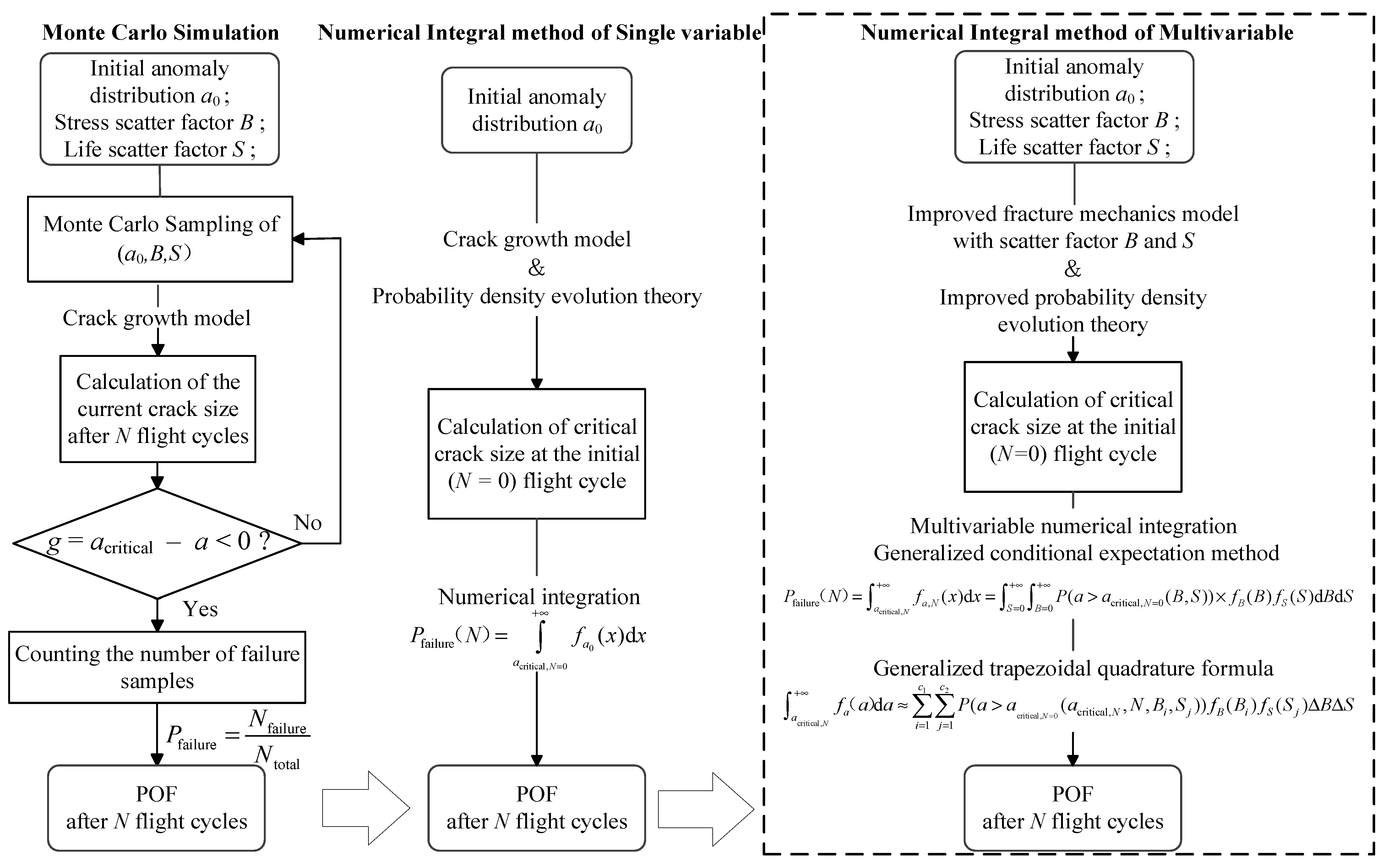
2.2. Mechanism of the Establishment of Multiple Integration in Multivariable PDTA

The probability density evolution theory is the basis of this work. It transforms the integral from the current N flight cycles into the initial (N = 0) flight cycles, which solves the core point by integrating at N flight cycles. First, Section 2.2.1 introduces the application of the theory of probability density evolution. Then, the mathematical demonstration of establishing multiple integrations considering random variables is described.

2.2.1. Probability Conservation and Spatial Transformation in the Theory of Probability Density Evolution

The principle of probability conservation is generally expressed through the evolution of conservative stochastic systems [38]. Some investigations [39,40,41] have implied or discussed the principle of conservation of probability in in-depth studies of the PDF solution of stochastic dynamical systems, i.e., to establish the relationship between the state PDF and the ‘initial’ PDF of random factors, the total probability is considered to be constant in the evolution process of the system [42]. These applications have proven the rationality of probability spatial transformation (from N flight cycles to the initial state) in this paper. A conservative stochastic system is one in which neither an existing random factor disappears nor a new random factor appears in the evolution process. In this problem, the stochastic dynamic system is involved in the crack growth system. The classical crack growth equations expressed in the form of a dynamic differential equation are as follows:

$$\stackrel{•}{a}=A(X,N),$$

(7)

where X = (a₀, B, S) is the state vector of the crack growth dynamic system, and only the crack size evolves over time. A(·) is a deterministic operator related to the crack growth rate, such as the Paris law shown in Equation (3). This dynamic system describes the temporal evolution of crack size as a differential equation. Thus, the classical Liouville equation can be expressed as follows:

$$\frac{\partial f_X(x,N)}{\partial N}+{\displaystyle \sum _1^3\frac{\partial [f_X(x,N)A(x,N)]}{\partial x_j}}=0,$$

(8)

where x is the realization of X. However, considerable effort is required to solve this partial differential equation. Instead of solving Equation (8), a multivariable NI method is proposed.

The preceding analysis shows that A is determined by the crack growth model in Equation (3) and the calculation model of the stress intensity factor in Equation (5). This dynamic equation establishes a one-to-one correspondence between the initial (N = 0) critical crack size $a_{\mathrm{critical}, N=0}$ and the critical crack size $a_{\mathrm{critical}, N}$ after N flight cycles, as shown in Figure 4. Based on probability conservation theory, when performing probability space transformations, the calculation system must satisfy a probabilistic conservation condition, and the entire evolutionary process must be monotonic, which means A(X, N)$\ge 0$ should always be true. In this paper, both Equation (7) and the physical meaning of the crack growth meet this requirement (the material cannot recover by itself once cracked).

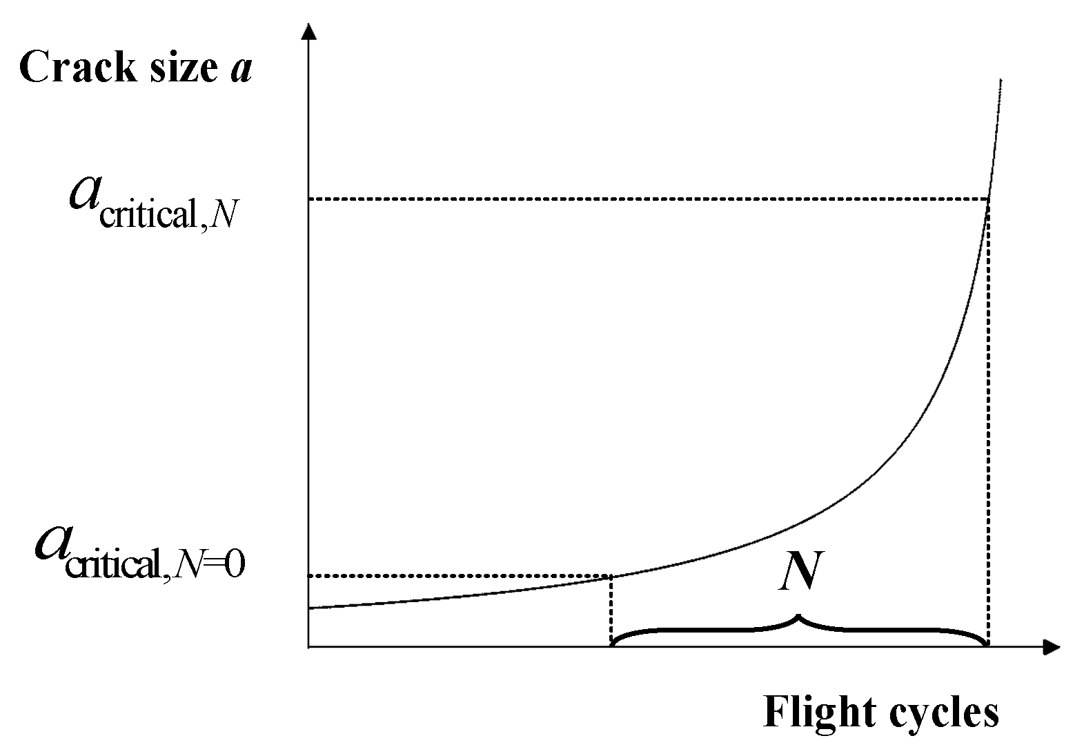
2.2.2. The Establishment of Multiple Integration in Multivariable PDTA

With the multiple random variables considered in the practical PDTA characterized in Section 2.1, disk failure is defined as a situation in which the crack size is larger than a critical size related to the load and material probability after N flight cycles. Hence, in terms of numerical calculations, the integral of the failure region [$a_{\mathrm{critical}, N}$, $+\infty$] is:

$$P_{\mathrm{f}}(N)=P(a>a_{\mathrm{critical},N}^{})={\displaystyle {\int }_{a_{\mathrm{critical},N}^{}}^{+\infty }{f}_{a,N}(a)\mathrm{d}a},$$

(9)

where $a_{\mathrm{critical}, N}$, is the critical crack size leading to disk fracture, and $f_{a, N}$ is the probability density of crack size after N cycles. However, in most cases, the crack size probability density $f_{a, N}$ after N cycles cannot be easily obtained. Consequently, probability density evolution theory is introduced. When stochastic systems maintain the conservation of probability and the entire process satisfies the monotonicity condition during evolution, the integral region can be transformed into the initial (N = 0) probability distribution space. Therefore, if the initial variables are mutually independent, the integral calculation is performed as follows:

$${\displaystyle {\int }_{a_{c,N}^{}}^{+\infty }{f}_{a,N}(a)\mathrm{d}a}={\displaystyle {\iiint }_{{\mathsf{\Omega }}_{\mathrm{f},N=0}}f(a_0,B,S)\mathrm{d}S\mathrm{d}B\mathrm{d}{a}_0}={\displaystyle {\iiint }_{{\mathsf{\Omega }}_{\mathrm{f},N=0}}{f}_{a_0}{f}_B{f}_S\mathrm{d}{a}_0\mathrm{d}B\mathrm{d}S},$$

(10)

where $a_0, B, S$ are the variables considered in the PDTA, $f_{a_0}{, f}_B{, f}_S$ are the probability densities of variables $a_0, B, S$ in the initial (N = 0) flight cycle, and ${\mathsf{\Omega }}_{\mathrm{f}, N=0}$ is the failure region to be integrated at the initial (N = 0) flight cycle. The definition of the failure region ${\mathsf{\Omega }}_{\mathrm{f}, N=0}$ ultimately provides the POF since the distribution of each initial variable is clear.

Furthermore, the generalised conditional expectation method proposed by Ayyub was proven reasonable and efficient for multivariable structural reliability assessment in 1992 [43]. Nevertheless, the solution of the control variable’s distribution function is not given in this research and is generally difficult to obtain. However, if the probability density evolution theory is introduced and the control variable varies from the defect size after N cycles to the initial (N = 0) defect size, the distribution function of the control variable can be directly obtained from the statistics of the initial defect size. Therefore, the crack size is chosen as the random control variable, and B and S become the conditional random variable set in Equation (10).

Moreover, the stochastic dynamic system involved in PDTA is a monotonic crack growth system, which means that all cracks exceeding the critical size of $a_{\mathrm{critical}, N=0}$ in the initial cycle (N = 0) are longer than the critical size of $a_{\mathrm{critical}, N}$ after N cycles when all other variables are constant. Hence, the failure region of ${\mathsf{\Omega }}_{\mathrm{f}, N=0}$ is limited to $\left\{{a|a >a}_{\mathrm{critical}, N=0}, N=0\right\}$, and the POF is eventually a form of conditional expectation. Equivalently, Equation (10) is rewritten as follows:

$${\displaystyle {\int }_{a_{\mathrm{critical},N}^{}}^{+\infty }{f}_{a,N}(a)\mathrm{d}a}={\displaystyle {\int }_{B=0}^{+\infty }{\displaystyle {\int }_{S=0}^{+\infty }P(a>a_{\mathrm{critical},N=0}^{}(B,S))\times f_B\times f_S\mathrm{d}B\mathrm{d}S}},$$

(11)

where $a_{\mathrm{critical}, N=0}$ is the initial (N = 0) critical crack size associated with each value of the conditional variables $\left\{B, S\right\}$ and is determined by inversely solving for the crack growth from the critical crack size $a_{\mathrm{critical}, N}$ after N cycles.

$${\displaystyle {\int }_{a_{{}_{\mathrm{critical},N}}^{}}^{+\infty }{f}_{a,N}(a)}\mathrm{d}a\approx {\displaystyle \sum _{i=1}^{c_1}{\displaystyle \sum _{j=1}^{c_2}P(a>a_{{}_{\mathrm{critical},N=0}}^{}(B_i,S_j))f_B(B_i)f_S(S_j)\mathrm{\Delta }B\mathrm{\Delta }S}}.$$

(12)

As shown in Equation (12), the general trapezoidal quadrature formula [44] is applied to solve the multiple integrals in Equation (11). The trapezoidal method is a standard method of performing definite multiple integral calculations. The integration region is divided into equal segments, and $\mathrm{\Delta }B$ and $\mathrm{\Delta }S$ are recorded as the sizes of the equally spaced intervals of the random variables $B$ and $S$. Additionally, $c_1$ and $c_2$ are the numbers of divided intervals for each variable, and $B_i$ and $S_j$ are the points in each interval.

This integral process is time-consuming if the number of variables in Equation (12) is large or if the step size is small. Indeed, multiple variables and a small step size lead to substantial crack growth computations that deserve analysis. Furthermore, the accuracy and efficiency of the NI method are affected by the step size. For example, if the integration step size is large, the accuracy becomes low. Nevertheless, the small integral step leads to an increase in the calculation cost accordingly. Hence, for the NI method’s efficiency analysis, the first step is to find a step size that results in convergence, similar to finding mesh-independent solutions in finite elements. Therefore, the NI method’s mechanism for augmenting the computational efficiency can be summarised in three parts: the number of variables, the efficiency of each crack growth computation, and the integration step size. Note that the crack growth calculation is included in different probabilistic calculation methods; thus, this model is not the focus of this paper.

The model of multiple integrals of the stochastic dynamical system is established by applying the probability density evolution theory, the generalized conditional expectation method, and the general trapezoidal quadrature formula.

2.3. The Multivariable NI Method of PDTA

This section presents the details of the analytical calculations in the risk assessment process in Figure 2. First, the zone and disk’s POF calculation models use critical analysis to achieve a complete risk assessment. Then, based on the input variables introduced above, the NI method’s implementation mechanism is emphasized.

2.3.1. Zone and Disk POF Calculation Model

The zone-based technique [45] is applied to address the uncertainty of crack location. This technique discretizes a disk into individual zones that generally have a constant stress and temperature state. The disk’s failure risk is the probability union of all zones’ POF. As the occurrence rate of hard-$\alpha$ is low, such that the probability of multiple defects in the unified zone is negligible [46], the disk’s POF $P_{\mathrm{f}, \mathrm{disk}}$ is approximated by the sum of the zone’s POF:

$$P_{\mathrm{f},\mathrm{disk}}\approx {\displaystyle \sum _{\mathrm{zone}=1}^M{\alpha }_{\mathrm{zone}}}\times P_{\mathrm{f},\mathrm{zone},\mathrm{cond}},$$

(13)

where ${\alpha }_{\mathrm{zone}}$ is the occurrence probability of hard-$\alpha$ inclusions related to each zone’s quality, $P_{\mathrm{f}, \mathrm{zone}, \mathrm{cond}}$ is the fracture probability under the condition of defect occurrence, and M is the number of zones.

The probabilistic failure risk assessment method introduces the engine structural failure probability concept and conducts risk analysis through probability statistics. The zone POF $P_{\mathrm{f}, \mathrm{zone}, \mathrm{cond}}$ is the conditional probability of fatigue fracturing due to the growth of cracks. In addition, according to probabilistic fracture mechanics theory, the critical condition for crack instability growth requires that the stress intensity factor K at the crack tip be larger than the material fracture toughness Kc. Thus, the probability of a structural fatigue fracture can be expressed as the probability of K > Kc in the following equation:

$$P_{\mathrm{f},\mathrm{zone}.\mathrm{cond}}=P(K>K_{\mathrm{c}}).$$

(14)

However, the stress intensity factor K cannot be measured from the base material experiment. Therefore, the probability distribution of K should be converted into the probability distribution of crack length. As a result, a one-to-one correspondence exists between the stress intensity factor K and the crack length. Thus, Equation (13) is equivalent to Equation (14).

$$P_{\mathrm{f},\mathrm{zone},\mathrm{cond}}=P(a>a_{\mathrm{critical},N}^{}).$$

(15)

This result implies that the fracture failure probability of the structure is the probability that the crack length is greater than the critical crack size of $a_{\mathrm{critical}, N}$ after N flight cycles. By applying the probability integration algorithm, Equation (15) can be expressed as the following equation:

$$P_{\mathrm{f},\mathrm{zone},\mathrm{cond}}={\displaystyle {\int }_{a_{{}_{\mathrm{critical},N}}^{}}^{+\infty }{f}_{a,N}(a)\mathrm{d}a},$$

(16)

where $f_{a, N}$ is the probability density function of the crack length after N flight cycles, and $a_{\mathrm{critical}, N}$ is the critical crack size at fracture.

Therefore, the structure’s failure probability can be determined by integration if $f_{a, N}$ and $a_{\mathrm{critical}, N}$ are known. The failure probability under different numbers of flight cycles N forms the failure probability curve.

2.3.2. The Implementation Algorithm of the Multivariable NI Method

According to Equation (16), if $a_{\mathrm{critical}, N}$ is found, the corresponding failure probability $P_{\mathrm{f}, \mathrm{zone}, \mathrm{cond}}$ can be determined. Using different fracture mechanics laws, the relationship between $a_{\mathrm{critical}, N=0}$ and $a_{\mathrm{critical}, N}$ can be obtained by the crack growth curve shown in Figure 4. For an initial crack size a₀, the integral solution of Equation (7) is G_N, and then the crack size a(N) after N flight cycles is

$$a(N)=G_N(a_0,N,B,S).$$

(17)

Then, conversely, if the critical crack size at fracture failure is $a_{\mathrm{critical}, N}$, the corresponding critical initial crack length $a_{\mathrm{critical}, N=0}$ is:

$$a_{\mathrm{critical},N=0}^{}=G_N^{-1}(a_{\mathrm{critical},N}^{},N,B,S).$$

(18)

If the shape factor Q in Equation (5) is approximated as a constant, then the Paris crack growth differential equation of Equation (3) has an analytical solution, as shown in Equation (19). Furthermore, the general form of the function G_N is the crack growth curve, as illustrated in Figure 4, by using the NASGRO law, the Forman model, or experimental data. Hence, the initial crack size $a_{\mathrm{critical}, N=0}$ can be obtained by interpolating the crack growth curve.

$$a_{\mathrm{critical},N=0}^{}={[{(a_{\mathrm{critical},N}^{})}^{1-\frac{n}{2}}-S\cdot C(1-\frac{n}{2}){(Q\cdot B\cdot \sigma \sqrt{\pi })}^n\cdot N]}^{\frac{2}{2-n}}.$$

(19)

In general, finding an analytical expression of the function G_N is difficult. However, this function is characterised by the physical laws of crack growth. Thus, the discrete data on crack growth obtained through experimental methods or finite element modelling can reflect the corresponding relationship with G_N, represented in the form of a plot, as shown in Figure 4.

Therein, the critical crack size $a_{\mathrm{critical}, N=0}$ obtained by Equation (5) according to the material fracture toughness Kc is shown as follows:

$$a_{\mathrm{critical},N}^{}=\frac{K_{\mathrm{c}}^2}{\pi {(Q\cdot B\cdot \sigma )}^2},$$

(20)

where B is the stress scatter factor, which describes the dispersion of the disk load $\sigma$.

An analysis of the physical meaning should precede the use of Equation (11) for probabilistic integration calculations. According to probability density evolution theory, Equation (11) describes the random variable’s spatial transformation relationship in different evolutionary stages. In reality, because this expression requires that A(X, N)$\ge 0$ in Equation (7) is always satisfied, the crack growth process is monotonic. This condition means that in the initial distribution, all of the cracks that are longer than the length of $a_{\mathrm{critical}, N=0}$ must remain longer than $a_{\mathrm{critical}, N}$ if the parameters B, S, and N are the same. This probability satisfies the conservation relationship.

Because the material initial defect information is known. The probability of the initial defect size exceeding $a_{\mathrm{critical}, N=0}$ is:

$$P(a_0>a_{\mathrm{critical},N=0}^{})=(1 - CDF(a_{\mathrm{critical},N=0}^{})),$$

(21)

where ${\mathit{CDF}(a}_{\mathrm{critical}, N=0})$ is the cumulative distribution function of the initial crack size. This function can be calculated from the exceedance probability data for the initial crack length shown in Figure 3 (denoted as exc(a₀)), as follows:

$$CDF(a_{\mathrm{critical},N=0}^{})=\frac{exc(a_{\mathrm{critical},N=0}^{})-exc(a_{0,\min })}{exc(a_{0,\max })-exc(a_{0,\min })},$$

(22)

After the theoretical analysis, the zone’s failure probability is obtained after the double numerical integration calculation. The main steps in this process are as follows. First, the critical crack length $a_{\mathrm{critical}, N}$ is determined at the time of fracture according to the material fracture toughness Kc, stress $\sigma$, and stress scatter factor B by Equation (9). Next, the corresponding initial critical crack length $a_{\mathrm{critical}, N=0}$ is obtained from the crack growth equation, i.e., Equation (8). Then, the conditional failure probability of the zone $P_{\mathrm{f}, \mathrm{zone}, \mathrm{cond}}$ is determined through Equation (6). Finally, the disk failure probability is computed utilizing Equation (3).

The significant advantage of this multivariable numerical integration method lies in the fact that it directly converts the probabilities of random variables in different evolutionary processes into spatial transformations, thereby significantly reducing unnecessary calculations.

3. Computational Model and Inputs

In this study, a centrifugal compressor disk model is applied to compare the convergence, accuracy, and efficiency of the PDTA process with different calculation methods. First, under the same boundary and life expectancy conditions, the failure probability of the disk is evaluated by the NI and MCS methods. Then, convergence, precision, and efficiency are compared and discussed. Additionally, to further clarify the NI method’s advantages, the importance sampling method [23] is considered.

This study presents the benefit of the NI method based on computational efficiency. The thermoelastic analysis process is not detailed in this paper because the stress and temperature of the disks obtained through prequel thermoelastic analysis are inputs for the PDTA. This section introduces the computational model and essential PDTA inputs.

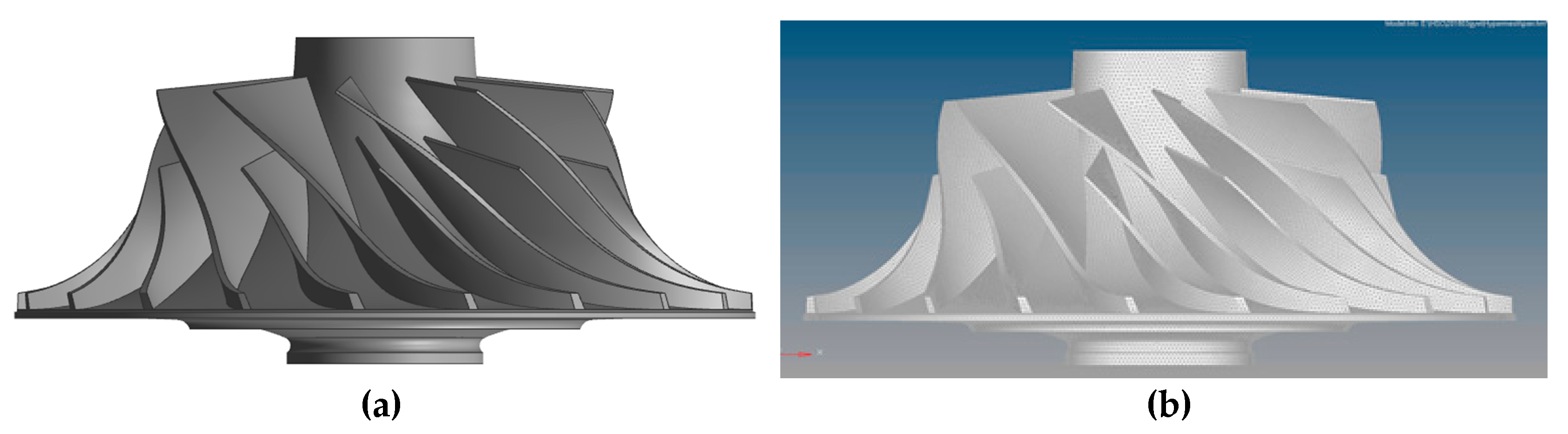
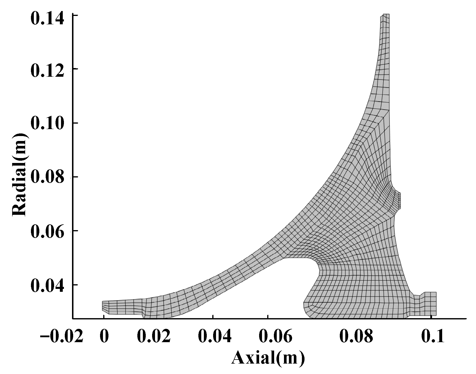
3.1. Computational Model

An actual centrifugal compressor disk model [47] is used, as presented in Figure 5. Once the disk’s stress and temperature during a flight cycle are obtained based on a 3D model, the PDTA is performed in the radial–axial cross-section. The aeroengine disk’s representative safety analysis process starts with aircraft and engine requirements, flight profile selection, and performance analysis. Load analysis in a flight cycle is then performed, followed by life and failure risk analysis. In the failure analysis, the defect is assumed to be a lamellar circular tension-type crack subjected to circumferential stress loading.

The boundary conditions in the steady state applied in the load analysis are shown in

Table 1. Boundary conditions in the steady state.

Boundary Conditions	Value
Disk rotation speed	35,000 rev/min
Mass Flow	6.825 × 10−5 kg/s
Inlet temperature	288.15 K
Outlet temperature	445.83 K
Outlet pressure	383 KPa

. The element type of the solid region is composed of tetrahedra elements of Solid45. The solid region’s finite element model consists of more than 2,140,291 units and 428,699 nodes to meet PDTA analysis requirements, requiring adequate nodes on the radial–axial section, as shown in Figure 5. That is, the mesh was refined after the grid-independent solution analysis. After the load analysis by finite element calculation, the node stress in the radial–axial section is interpolated into a new quadrilateral mesh for PDTA analysis. The new quadrilateral mesh is shown in Figure 6. Detailed information on finite element analysis can be found in Ref. [47]. The material parameters of Ti6Al4V are listed in

Table 2. The material parameters of Ti6Al4V.

Parameters	Value
Density	4450 kg/m3
Young’s modulus	120,000 MPa
Poisson’s ratio	0.361
da/dN	9.25 × 10−13(ΔK) 3.87 m/cycle
K threshold	0.0 MPa√m
Fracture toughness	64.5 MPa√m
Yield strength	834 MPa

. These data are taken from Ref. [47], including generic Ti6Al4V Paris fit data [15].

3.2. Inputs for the PDTA

Based on the integrated process of a typical PDTA with multiple variables considered, the inputs of the POF calculation other than material properties include the stress distribution and zone definition, defect material anomaly distribution (determining the initial defect size of the material), design service life, life scatter factor, and stress scatter factor. The analysis occurs as follows.

(1) Stress distribution and zone definition

The disk is divided into zones based on the stress distribution of the meridional surface, as shown in Figure 7. The stress in the figure shows the circumferential stress distribution. A zone is considered to be a grouping of materials such that all subregions in the zone have a generally uniform stress state, the same properties of fatigue crack growth, inspection schedules, probability of detection curves, and anomaly distribution [47]. The life of a zone is approximately constant for a given initial crack size. In other words, the risk computed for any subregion of the zone’s material will be the same [47]. According to the principle of stress similarity, finite elements are grouped into a specific stress interval zone. That is, the circumferential stress is extracted for zone definition. The finite elements are then differentiated into different zones by classifying the element stress into different stress intervals. These stress intervals are divided into equal intervals from the disk’s minimum stress to the maximum stress. As shown in Figure 7b, stress intervals of 34.5 MPa are practical and adequate for the initial zone definition suggested by Advisory Circular 33.14-1 [14]. Analytical convergence requires further zone refinement [25], which will increase the number of zones and result in a subsequent increase in computing. Therefore, 34.5 MPa is considered the stress interval in this paper [14]. Surface and corner zones are defined to consider anomalies/cracks located in near-surface regions that generally grow faster than embedded cracks under the same load conditions. Hence, three types of zones are considered in this study: zones containing embedded cracks, zones containing surface cracks, and zones containing corner cracks.

(2) Defect material anomaly distribution (determining the initial defect size of material)

The “Post 1995 Triple Melt/Cold Hearth + VAR Hard Alpha Inclusion Distribution” [14] data shown in Figure 3 contain information on the initial anomaly size distribution. For the NI method, the distribution data (per million pounds) can be used directly on a volumetric basis (per cubic meter) by multiplying the material’s density. Note that the uncertainty of the initial defect size discussed in Section 2.2 is contained in this anomaly distribution, which is one of the variables considered in this paper.

(3) Life scatter factor and stress scatter factor

The life scatter factor S reflects the dispersion of the crack growth rate. In this paper, S follows a log-normal distribution with a median value equal to 1 and 20% COV (coefficient of variation). The stress scatter factor B describes the uncertainty of the disk stress. B follows a log-normal distribution with a median value equal to 1 and 20% COV.

(4) Design service life

The design service is the input of PDTA. Based on a particular engine design, the design service life is 20,000 flight cycles in this case.

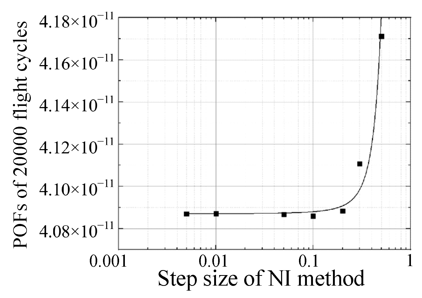
3.3. Considered Cases for Converge Result

The convergence, accuracy, and efficiency of the different methods are now compared. The NI method and MCS are first applied for comparison. The importance sampling method is also considered to emphasise the advantage of the NI method.

For the NI method, the analysis process is given in Section 2.3. However, it should be noted that the computational efficiency and precision of the NI method are affected by the integration step size. That is, only the converged integral results under a sufficiently small integration step size are comparable. Thus, seven cases with different step sizes of 0.005, 0.01, 0.05, 0.1, 0.2, 0.3, and 0.5 were chosen to obtain the convergence accuracy. Another relevant point concerns the integral region in Equation (11). To meet the precision requirement, [1.5σ, 12.5σ] was selected as the integration region in the seven NI method cases, where σ is the standard deviation. The integration ranges are not static for the scatter factors of different statistical distributions. In this paper, the integral region is large enough because the error between the joint probability density integration and 1 is below 10⁻⁶. For other problems, considering different variables with different statistical distributions, the integration region can be determined by calculating the integral area of the joint probability density of the scatter factors in the limited integral region. For the MCS, the number of samples is a crucial factor influencing the calculation efficiency. Hence, 15 cases were explored within the range of 10⁵ to 5 × 10⁷ sample size to analyse the results’ convergence. Additionally, the importance sampling method similar to the method introduced in reference [23] is used to compare it with the NI method, indicating that only those samples that fail are generated, and eight cases were considered.

For the abovementioned methods, the same simplified Paris law and Newman method were used to achieve a uniform calculation cost of fatigue crack growth [34,37]. All of the cases considered were investigated on a single central processing unit (CPU) in the same computer to compare the algorithm performance for each method (the NI method, MCS, and importance sampling method). The CPU version is an Intel(R) Core (TM) i7-8700 CPU with a 3.20 GHz processor. A Windows^® platform software package self-developed with the Microsoft Foundation Classes (MFC) library was used for the evaluation and analysis. Furthermore, calculation time was selected as the indicator of computational cost, given that time cost is the most intuitive way to evaluate and understand the efficiency of methods.

4. Results and Discussion

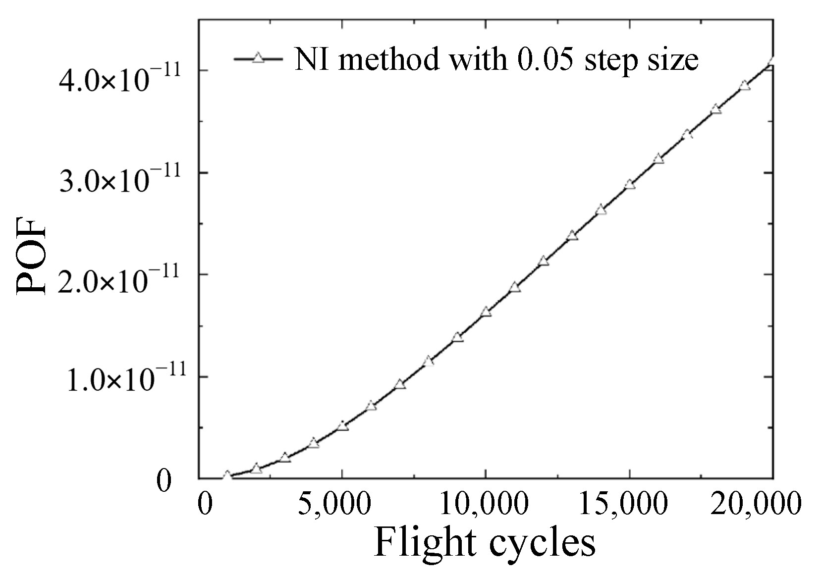
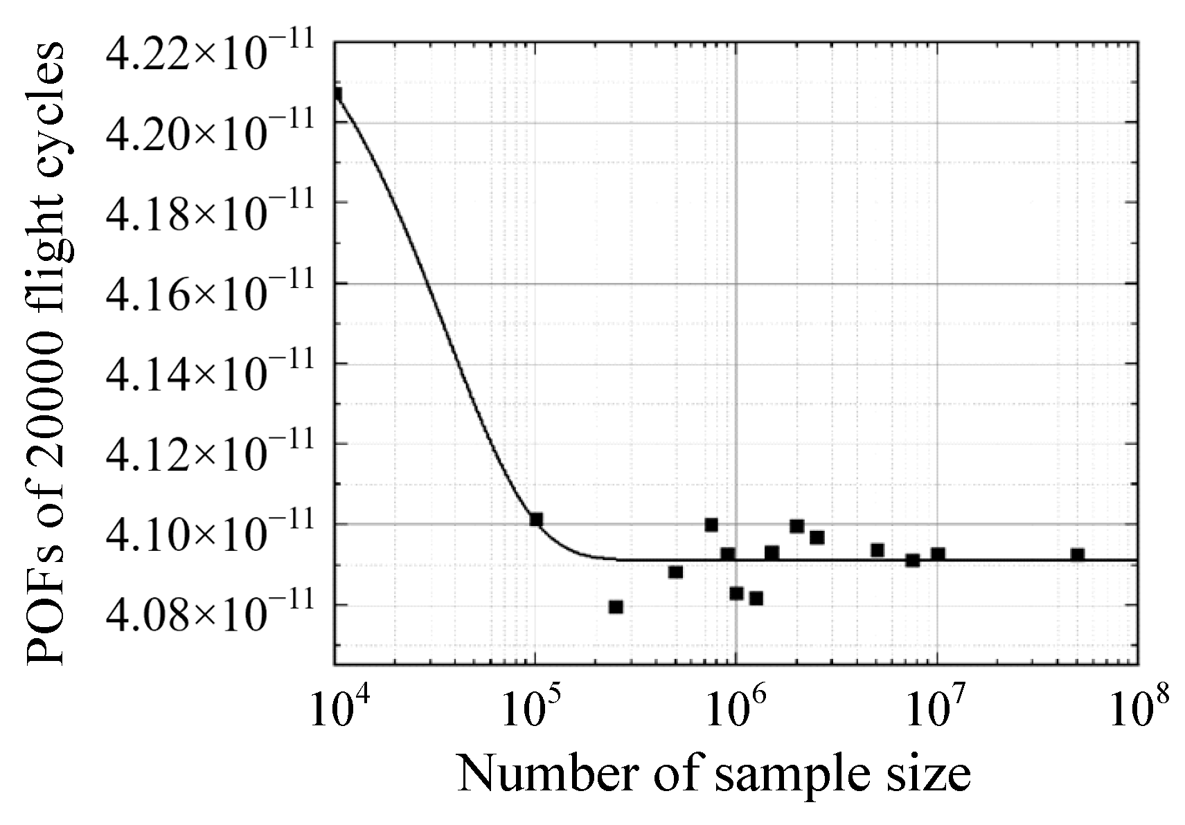
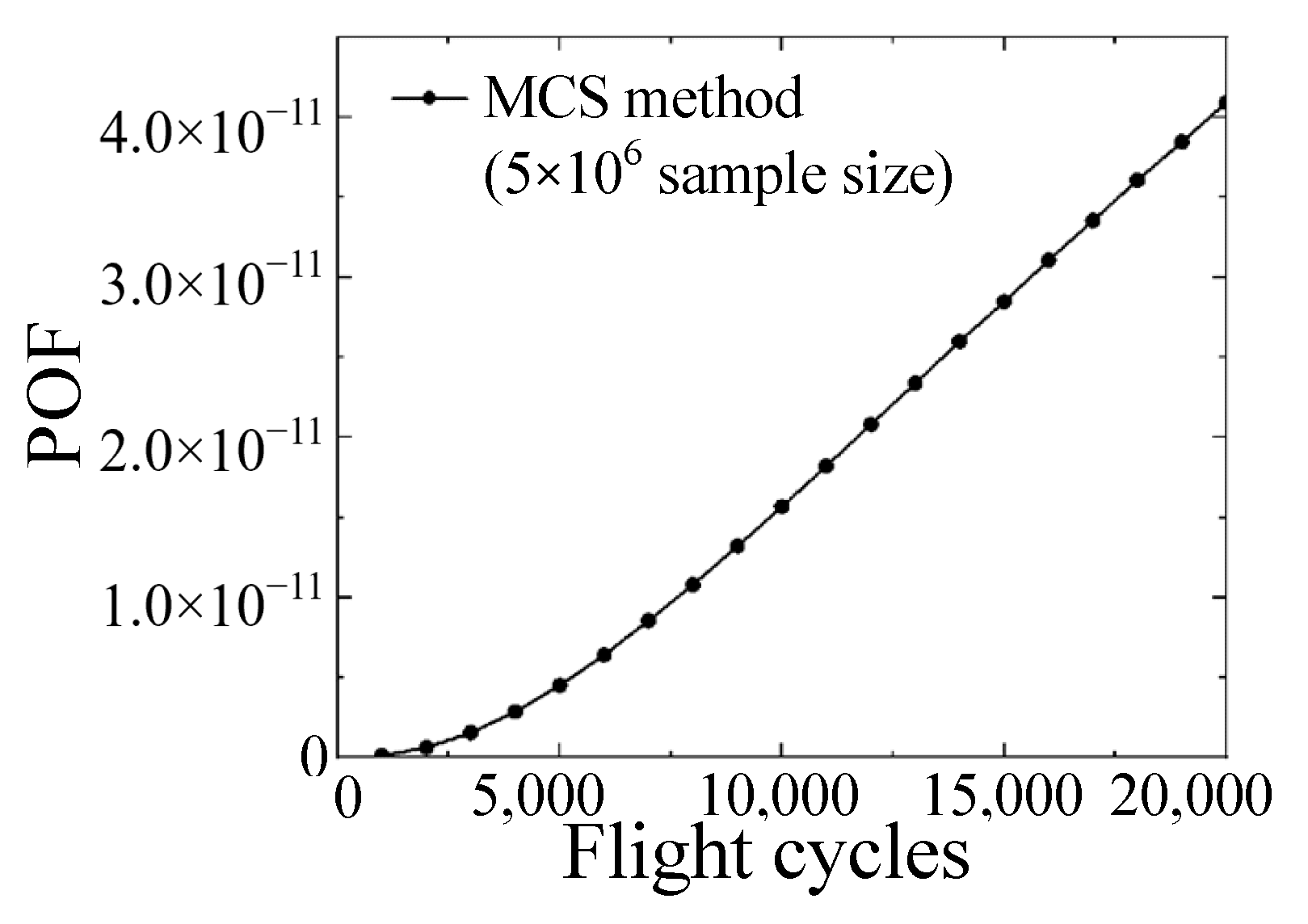
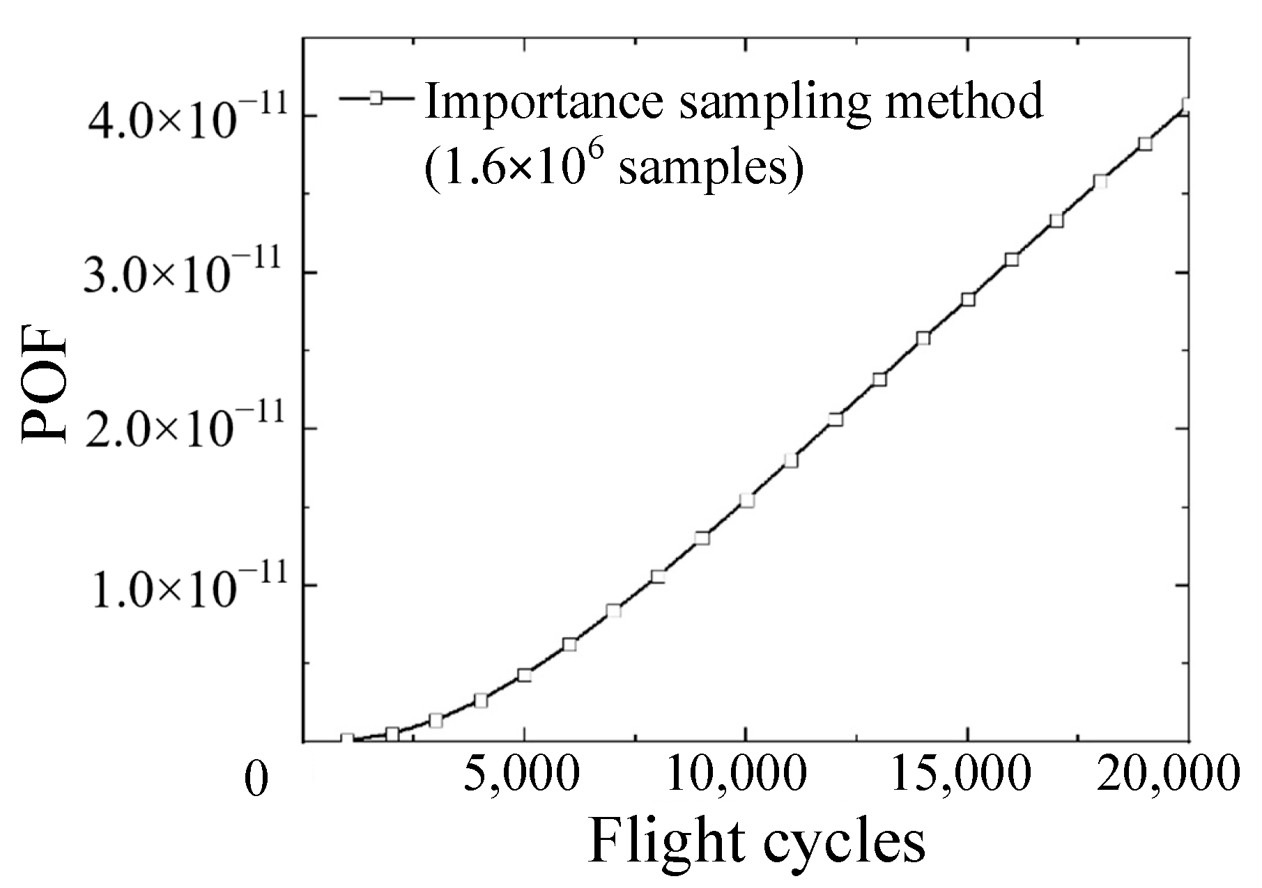
4.1. Convergence Results with Different Methods

As stated previously, to compare the convergence, accuracy and efficiency of different methods, the convergence of the results should be discussed first. The results of the different calculation cases are as follows.

(1) Cases with the NI method for different step sizes

The POFs (events/cycle) at 20,000 flight cycles are used as an indicator to estimate the convergence. From Figure 8, the results converge as the integral step size decreases. However, the NI method’s calculation time cost increases with decreasing step size, as shown in Figure 9. That is, the integration step size affects both the integration accuracy and the calculation time cost. If the integration step size is large, then the accuracy becomes low.

Nevertheless, the small integral step can increase the calculation cost, as shown in Figure 8. Similar to finding the grid-independent solution in finite element analysis, the first step of applying the NI method is to find a step size that results in convergence, which is a step size of less than 0.05. Moreover, although stress factor B and life scatter factor S have different units, the integral converges as the step size is less than 0.05, as illustrated in Figure 8. One of the NI method’s advantages is that the result converges rapidly with a decreasing step size. The calculation results are fitted with an exponential curve, and the results of the NI method converge when the step size is less than 0.05. Hence, to compare the NI method’s calculation efficiency with that of the MCS and importance sampling methods, the POF curve (step size of 0.05) with the lowest time cost in the convergent cases is presented in Figure 10.

(2) Cases with MCS for different sample sizes

Similarly, to determine the number of samples needed for MCS convergence, fifteen cases with sample sizes from 10⁴ to 5 × 10⁷ were investigated. According to the exponential fitting curve shown in Figure 11, the results converge to a stable value as the number of samples exceeds 5 × 10⁶. Before this threshold, the error caused by the small sample size led to a fluctuation in the results around the convergence value, which is one of the inevitable shortcomings of MCS. The designed target risk is a design parameter generally small for an actual engine disk, for example, 10⁻⁹ events per flight cycle for component-level design target risk value [14]. Thus, the requirement for the number of MCS samples reaches millions. Large quantities of sample calculations result in high computational costs, as shown in Figure 12. This study considers MCS results with a sample size larger than 5 × 10⁶ convergent. The POF curve obtained by MCS with a 5 × 10⁶ sample size, as shown in Figure 13, has the lowest time cost among those in all convergence cases.

(3) Cases with the importance sampling method for different sample sizes

The importance sampling method reduces the number of MCS samples by sampling only in the areas likely to experience failure [23]. In other words, the importance sampling method is an improved MCS approach, and its efficiency is affected by the number of samples, as is the conventional MCS. Herein, eight cases with different sample sizes from 1.8 × 10⁵ to 1.8 × 10⁷ were investigated to obtain a convergence result. Figure 14 shows that sample sizes larger than 1.6 × 10⁶ result in convergence. The time costs of different cases are shown in Figure 15. The POF curve with the lowest cost of convergence based on time is shown in Figure 16.

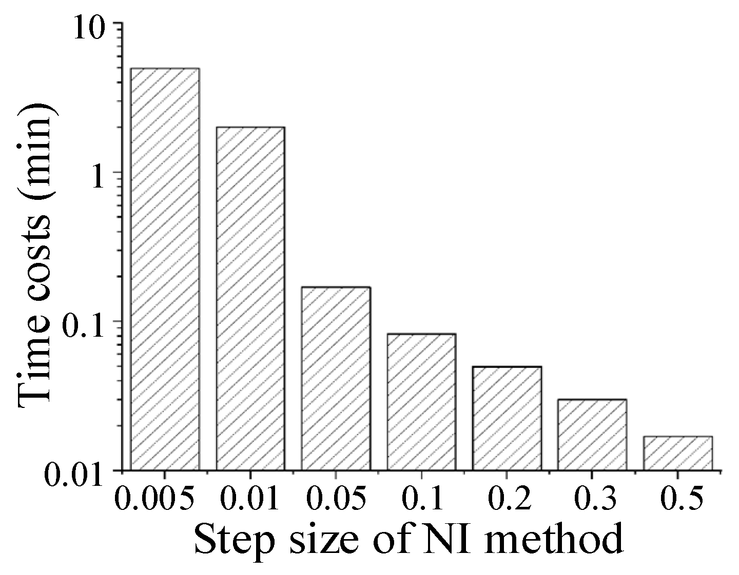
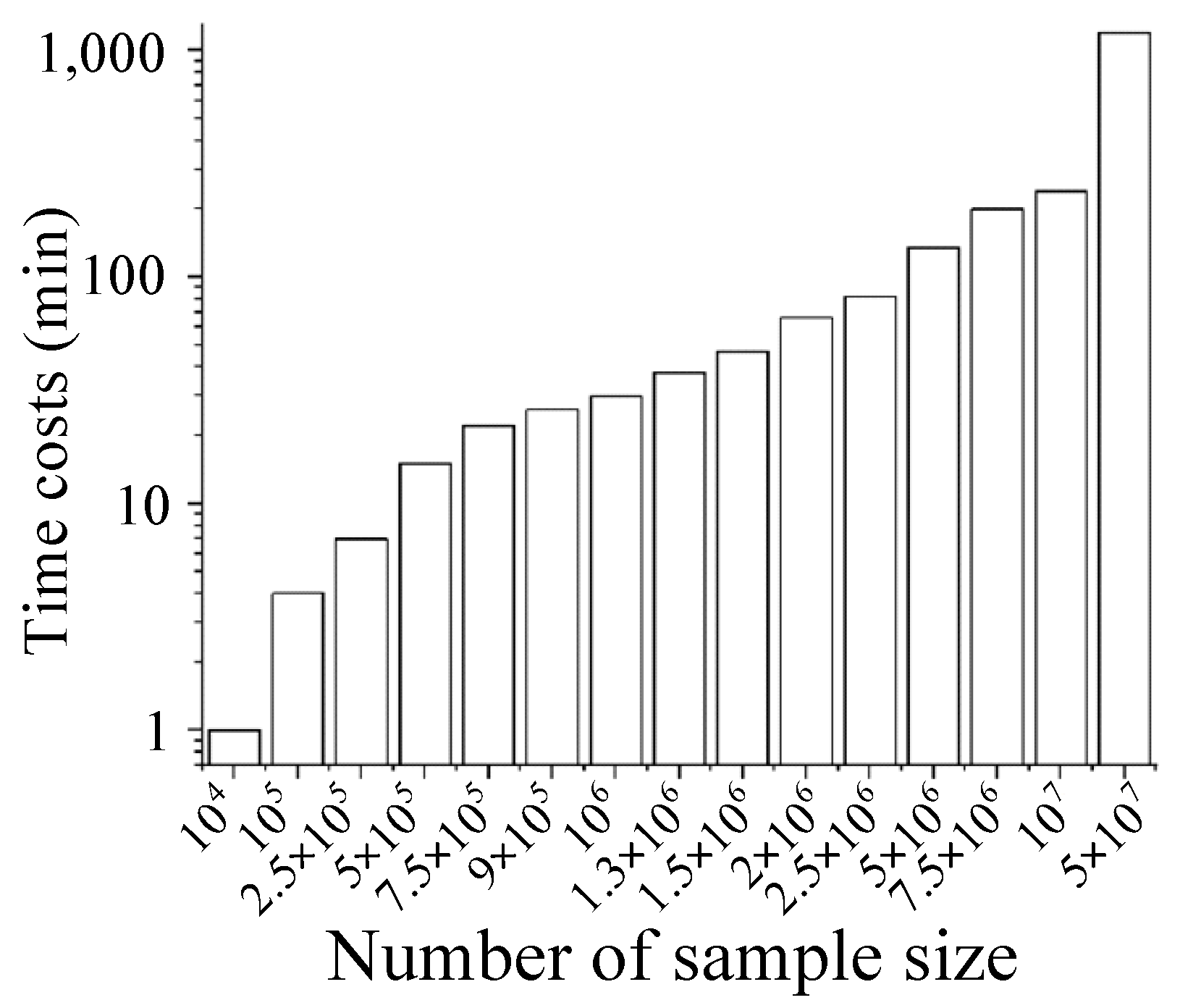
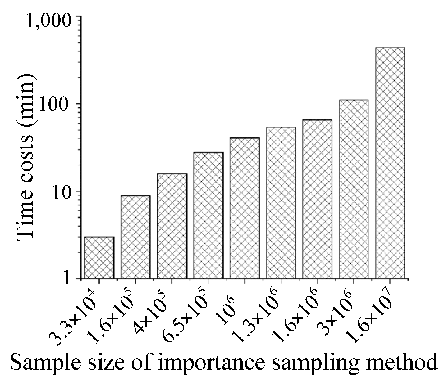
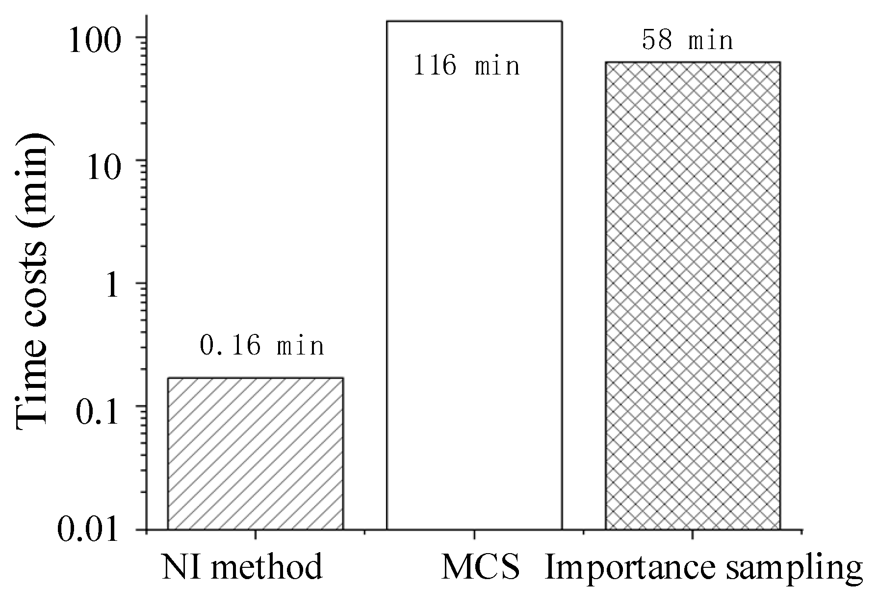
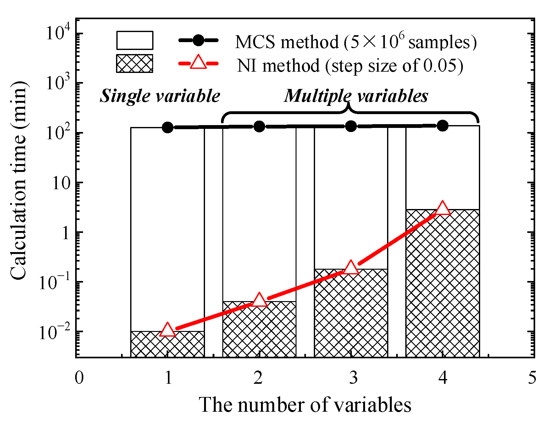
4.2. Comparison of Computational Costs and Precision with Different Methods

(1) Comparison of the computational costs of different methods

The NI method’s computational cost is compared with that of MCS, and the importance sampling method provides a clear understanding of the NI method. Based on the analysis above, convergence conditions are used for comparison; notably, the NI method has a 0.05 step size, MCS has a 5 × 10⁶ sample size, and the importance sampling method has a 1.6 × 10⁶ sample size. Figure 17 indicates that the NI method has an advantage over MCS and the importance sampling method in the calculation efficiency of the PDTA process. In addition, the NI method’s time cost is hundreds of times lower than that of MCS and the importance sampling method.

(2) Comparison of the computational precision of different methods

Theoretically, the NI method and MCS are entirely equivalent concerning the POF results. In other words, the result of the NI method is a numerical solution, and the MCS result converges to that of the NI method if the sample size is sufficiently large. However, there is a difference between the NI method and the MCS method, as shown in Figure 18, especially for a small number of flight cycles. This difference is related to the numerical algorithms and can be improved in subsequent studies; however, there is no notable impact on this paper’s conclusions. Although the corresponding precision is slightly better than the NI method, the efficiency is lower for the importance sampling method. The POF results at 20,000 flight cycles are shown in

Table 3. POFs at 20,000 flight cycles for different methods.

Calculation Method	POF at 20,000 Flight Cycles
NI method (step size of 0.05)	4.0867 × 10−11
MCS (sample size of 5 × 106)	4.0936 × 10−11
Importance sampling method (sample size of 1.5 × 106)	4.0777 × 10−11

. A maximum relative error of 0.2% exists between the NI method and the importance sampling method.

4.3. Discussion

Some conclusions can be summarised based on a comparison of the convergence, accuracy, and time costs of the NI method, MCS, and importance sampling method. Similar to the conclusion in the study of the fast NI algorithm [29], there is no significant difference between the results of the methods mentioned. It is emphasised that, for the typical PDTA process, the NI method’s calculation efficiency is superior to that of MCS and the importance sampling method under limited variable conditions.

Although the calculation cost is affected by the integration step size, convergence quickly occurs with the NI method’s reduction in the step size. MCS and the importance sampling method may be more efficient than the NI method when the number of variables is sufficiently large. The number of samples significantly impacts the two methods’ time cost, especially when the POF result is low, for instance, 10⁻¹¹ in this study. The demand for a large sample size leads to a high computational cost, which is the essential restriction of sampling calculations. Under finite variable conditions and several iterative optimisation analyses, the NI method makes additional scenes a characteristic requirement of PDTA in the design stage.

The NI method is a general efficiency probability calculation method regarding other components or applications. The crack growth model is the core of the probability damage tolerance assessment. Accordingly, the NI method’s critical step is to determine the initial crack size by reversely solving the crack growth equation. In addition, the NI method is applicable for other variables considered in the form of a scatter factor, such as material fracture toughness. Hence, the NI method is a general PDTA method.

Furthermore, to provide a clear understanding of the NI method’s efficiency with the increase in variable dimension, we conducted an additional study regarding the influence of variable dimension on POFs. It can be seen from Figure 19 that the time cost of the NI method is increased exponentially with an enlarged number of variables. In contrast, the time cost of MCS is not affected by the number of variables. Nevertheless, the number of variables in the practical PDTA is limited. Hence, the NI method proposed in this paper performs better than MCS in POF calculations.

Therefore, it is conceivable that the mechanism of the NI method is appropriate for most typical PDTA processes and contributes to improving the calculation efficiency.

5. Conclusions

This paper proposes a multivariable NI method based on probability density evolution to solve the computational efficiency problem of MCS and the improved MCS method in failure risk assessment considering multiple variables. A centrifugal compressor disk model is applied, and the corresponding results are compared with those of MCS and the importance sampling method to analyse the convergence, precision, and efficiency of this method. As a result, the following conclusions are obtained.

The probability density evolution algorithm can be applied for risk assessment under multivariate conditions. By establishing the relationship model between the initial probability distribution (N = 0) and the actual distribution after N flight cycles, this algorithm solves the limitation of MCS for large numbers of samples.

The method’s precision was verified by the cases performed in this paper. The NI method’s results convergence quickly occurs with the reduction in the step size. Compared with the MCS results, the proposed algorithm has a calculation efficiency that is 100 times better under the same input conditions and calculation precision.

The multivariable NI method provides a new algorithm for risk assessment POF calculation. Further studies considering non-destructive inspection in POF risk assessment are recommended.

Under the trend of continuous expansion of the civil aviation fleet, despite the fact that the accident rate is not high, the volume of civil aviation accidents should not increase in absolute terms. This requires that the safety of future aircraft and aeroengine must be continuously improved. Therefore, developing rotor probabilistic damage tolerance assessment of the aeroengine has essential value.

The challenges and future direction of probabilistic damage tolerance assessment are as follows. First, to accurately describe the stochastic nature of the harsh operating environment of the rotor disk and the temperature stress field it brings. Second, to solve the problem of the inhomogeneity of the material as well as the residual stresses due to the dispersion of rotor disc material composition and manufacturing process. Finally, to closely couple the PDTA with the operation and maintenance process to realise the quantitative calculation of the failure risk of the whole life process and lay the foundation for the real-time risk digital twin technology of the single engine.

References

1. Vittal, S.; Hajela, P.; Joshi, A. Review of Approaches to Gas Turbine Life Management. In Proceedings of the 10th AIAA/ISSMO Multidisciplinary Analysis and Optimization Conference, Albany, NY, USA, 30 August–1 September 2004. [Google Scholar]
2. Kadau, K.; Enright, M.; Amann, C. Probabilistic Lifing. In Handbook of Nondestructive Evaluation 4.0; Meyendorf, N., Ida, N., Singh, R., Vrana, J., Eds.; Springer International Publishing: Cham, Switzerland, 2021; pp. 1–38. ISBN 978-3-030-48200-8. [Google Scholar]
3. Enright, M.P.; Moody, J.P.; Zaman, Y.; Sobotka, J.C.; McClung, R.C. A Probabilistic Framework for Minimum Low Cycle Fatigue Life Prediction. In Proceedings of the ASME Turbo Expo 2022: Turbomachinery Technical Conference and Exposition, Rotterdam, The Netherlands, 13–17 June 2022; p. V08BT25A001. [Google Scholar]
4. Federal Aviation Administration. Advisory Circular—Damage Tolerance of Hole Features in High-Energy Turbine Engine Rotors; Federal Aviation Administration, U.S. Department of Transportation: Washington, DC, USA, 2009; AC 33.70-2.
5. European Aviation Safety Agency, Certification Specifications and Acceptable Means of Compliance for Large Aeroplanes. Amendment, 14. 2012. Available online: https://www.easa.europa.eu/en/document-library/easy-access-rules/easy-access-rules-engines-cs-e (accessed on 7 February 2020).
6. Li, J.X. CCAR-33-R2 Provisions on Airworthiness of Aircraft Engines; Civil Aviation Administration of China, Bulletin of the State Council of the People’s Republic of China: Beijing, China, 2016. Available online: http://www.caac.gov.cn/XXGK/XXGK/index_172.html?fl=12 (accessed on 17 March 2016).
7. Enright, M.P.; Moody, J.P.; Chandra, R.; Pentz, A.C. Influence of Mission Variability on Fracture Risk of Gas Turbine Engine Components. In Proceedings of the ASME Turbo Expo 2012: Turbine Technical Conference and Exposition, Copenhagen, Denmark, 11–15 June 2012; pp. 439–446. [Google Scholar]
8. Enright, M.P.; Huyse, L. Methodology for Probabilistic Life Prediction of Multiple-Anomaly Materials. AIAA J. 2006, 44, 787–793. [Google Scholar] [CrossRef]
9. Enright, M.P.; McClung, R.C.; Liang, W.; Lee, Y.-D.; Moody, J.P.; Fitch, S. A Tool for Probabilistic Damage Tolerance of Hole Features in Turbine Engine Rotors. In Proceedings of the ASME Turbo Expo 2012: Turbine Technical Conference and Exposition, Copenhagen, Denmark, 11–15 June 2012; pp. 447–458. [Google Scholar]
10. Chan, K.S.; Enright, M.P.; Moody, J.; Thomas, C.; Goodrum, W. HOTPITS: The DARWIN Approach to Assessing Risk of Hot Corrosion-Induced Fracture in Gas Turbine Components. Eng. Fract. Mech. 2020, 228, 106889. [Google Scholar] [CrossRef]
11. McClung, R.C.; Enright, M.P.; Moody, J.P.; Lee, Y.D.; McFarland, J. Integrating Fatigue Crack Growth into Reliability Analysis and Computational Materials Design. Adv. Mater. Res. 2014, 891–892, 1009–1014. [Google Scholar] [CrossRef]
12. Enright, M.P.; McClung, R.C.; Chan, K.S.; McFarland, J.; Moody, J.P.; Sobotka, J.C. Micromechanics-Based Fracture Risk Assessment Using Integrated Probabilistic Damage Tolerance Analysis and Manufacturing Process Models. In Proceedings of the ASME Turbo Expo 2016: Turbomachinery Technical Conference and Exposition, Seoul, South Korea, 13–17; June 2016; p. V07BT29A004. [Google Scholar]
13. Enright, M.P.; McClung, R.C. A Probabilistic Framework for Gas Turbine Engine Materials with Multiple Types of Anomalies. J. Eng. Gas Turbines Power 2011, 133, 082502. [Google Scholar] [CrossRef]
14. Federal Aviation Administration. Advisory Circular—Guidance Material for Aircraft Engine Life-Limited Parts Requirements; Federal Aviation Administration, U.S. Department of Transportation: Washington, DC, USA, 2009; AC 33.70-1.
15. Federal Aviation Administration. Advisory Circular—Damage Tolerance for High Energy Turbine Engine Rotors; Federal Aviation Administration, U.S. Department of Transportation: Washington, DC, USA, 2001; AC 33.14-1.
16. Millwater, H.; Ocampo, J.D.; Castaldo, A. Probabilistic Damage Tolerance Analysis for General Aviation. Adv. Mater. Res. 2014, 891–892, 1191–1196. [Google Scholar] [CrossRef]
17. Wu, Y.-T. Computational Methods for Efficient Structural Reliability and Reliability Sensitivity Analysis. AIAA J. 1994, 32, 1717–1723. [Google Scholar] [CrossRef]
18. Su, B.; Zhou, Q. A Semi-Analytical and Monte Carlo-Based Phase Dynamic Evolution Approach for LEO Mega-Constellations. Aerospace 2022, 9, 128. [Google Scholar] [CrossRef]
19. Jing, H.; Jian, C.; Liu, L. An Efficient Method of Calculating Stress Intensity Factor for Surface Cracks in Holes Under Uni-Variant Stressing. In Methods and Applications for Modeling and Simulation of Complex Systems; Fan, W., Zhang, L., Li, N., Song, X., Eds.; Communications in Computer and Information Science; Springer Nature Singapore: Singapore, 2022; Volume 1713, pp. 14–25. ISBN 978-981-19919-4-3. [Google Scholar]
20. Amann, C.; Kadau, K. Numerically Efficient Modified Runge–Kutta Solver for Fatigue Crack Growth Analysis. Eng. Fract. Mech. 2016, 161, 55–62. [Google Scholar] [CrossRef]
21. L’Ecuyer, P.; Simard, R.; Chen, E.J.; Kelton, W.D. An Object-Oriented Random-Number Package with Many Long Streams and Substreams. Oper. Res. 2002, 50, 1073–1075. [Google Scholar] [CrossRef] [Green Version]
22. Kadau, K.; Gravett, P.W.; Amann, C. Probabilistic Fracture Mechanics for Heavy-Duty Gas Turbine Rotor Forgings. J. Eng. Gas Turbines Power 2018, 140, 062503. [Google Scholar] [CrossRef]
23. Huyse, L.; Enright, M. Efficient Statistical Analysis of Failure Risk in Engine Rotor Disks Using Importance Sampling Techniques. In Proceedings of the 44th AIAA/ASME/ASCE/AHS/ASC Structures, Structural Dynamics, and Materials Conference, Norfolk, VA, USA, 7–10 April 2003. [Google Scholar]
24. Enright, M.P.; Millwater, H.R.; Huyse, L. Adaptive Optimal Sampling Methodology for Reliability Prediction of Series Systems. AIAA J. 2006, 44, 523–528. [Google Scholar] [CrossRef]
25. Millwater, H.; Enright, M.; Fitch, S. A Convergent Probabilistic Technique for Risk Assessment of Gas Turbine Disks Subject to Metallurgical Defects. In Proceedings of the 43rd AIAA/ASME/ASCE/AHS/ASC Structures, Structural Dynamics, and Materials Conference, Denver, CO, USA, 22–25 April 2002. [Google Scholar]
26. Enright, M.; Millwater, H.; Moody, J. Efficient Integration of Sampling-Based Spatial Conditional Failure Joint Probability Densities. In Proceedings of the 48th AIAA/ASME/ASCE/AHS/ASC Structures, Structural Dynamics, and Materials Conference, Honolulu, HI, USA, 23–26 April 2007. [Google Scholar]
27. Enright, M.; Millwater, H. Optimal Sampling Techniques for Zone-Based Probabilistic Fatigue Life Prediction. In Proceedings of the 43rd AIAA/ASME/ASCE/AHS/ASC Structures, Structural Dynamics, and Materials Conference, Denver, CO, USA, 22–25 April 2002. [Google Scholar]
28. Orisamolu, I.; Luo, X.; Orisamolu, I.; Luo, X. Probabilistic Assessment of Corrosion Effects on the Damage Tolerance of Aircraft Structures. In Proceedings of the 38th Structures, Structural Dynamics, and Materials Conference, Kissimmee, FL, USA, 7–10 April 1997. [Google Scholar]
29. Yang, L.; Ding, S.; Wang, Z.; Li, G. Efficient Probabilistic Risk Assessment for Aeroengine Turbine Disks Using Probability Density Evolution. AIAA J. 2017, 55, 2755–2761. [Google Scholar] [CrossRef]
30. Leverant, G.R.; Littlefield, D.L.; McClung, R.C.; Millwater, H.R.; Wu, J.Y. A Probabilistic Approach to Aircraft Turbine Rotor Material Design. In Proceedings of the ASME 1997 International Gas Turbine and Aeroengine Congress and Exhibition, Orlando, FL, USA, 2–5 June 1997; p. V004T14A010. [Google Scholar]
31. Wu, Y.-T.; Enright, M.P.; Millwater, H.R. Probabilistic Methods for Design Assessment of Reliability with Inspection. AIAA J. 2002, 40, 937–946. [Google Scholar] [CrossRef]
32. Millwater, H.R.; Fitch, S.H.K.; Wu, Y.-T.; Riha, D.S.; Enright, M.P.; Leverant, G.R.; McClung, R.C.; Kuhlman, C.J.; Chell, G.G.; Lee, Y.-D. A Probabilistically-Based Damage Tolerance Analysis Computer Program for Hard Alpha Anomalies in Titanium Rotors. In Proceedings of the ASME Turbo Expo 2000: Power for Land, Sea, and Air, Munich, Germany, 8–11 May 2000; p. V004T03A062. [Google Scholar]
33. Aerospace Industries Association Rotor Integrity Sub-Committee. The development of anomaly distributions for aircraft engine titanium disk alloys. In Proceedings of the 38th AIAA/ASME/ASCE/AHS/ASC Structures, Structural Dynamics, and Materials Conference, Kissimmee, FL, USA, 7–10 April 1997. [Google Scholar]
34. Raju, I.S.; Newman, J.C. A Reinvestigation of Stress-Intensity Factors for Surface and Corner Cracks in Three-Dimensional Solids. In Contemporary Research in Engineering Science; Batra, R.C., Ed.; Springer: Berlin/Heidelberg, Germany, 1995; pp. 418–441. ISBN 978-3-642-80003-0. [Google Scholar]
35. Glinka, G.; Shen, G. Universal Features of Weight Functions for Cracks in Mode I. Eng. Fract. Mech. 1991, 40, 1135–1146. [Google Scholar] [CrossRef]
36. Huang, X.; Chen, C.; Xuan, H.; Guo, X.; Shan, X.; Hong, W. Fatigue Crack Propagation Analysis in an Aero-Engine Turbine Disc Using Computational Methods and Spin Test. Theor. Appl. Fract. Mech. 2023, 124, 103745. [Google Scholar] [CrossRef]
37. Paris, P.; Erdogan, F. A Critical Analysis of Crack Propagation Laws. J. Basic Eng. 1963, 85, 528–533. [Google Scholar] [CrossRef]
38. Li, J.; Chen, J. Advances in The Research on Probability Density Evolution Equations of Stochastic Dynamical Systems. Adv. Mech. 2010, 40, 170–188. [Google Scholar] [CrossRef]
39. Lasota, A.; Mackey, M.C.; Chaos, F. Noise: Stochastic Aspects of Dynamics. Appl. Math. Sci. 1994, 97, 37–49. [Google Scholar]
40. Bontempi, F.; Casciati, F. Chaotic Motion and Stochastic Excitation. Nonlinear Dyn. 1994, 6, 179–191. [Google Scholar] [CrossRef]
41. Kozin, F. On the Probability Densities of the Output of Some Random Systems. J. Appl. Mech. 1961, 28, 161–164. [Google Scholar] [CrossRef]
42. Li, J.; Chen, J. The Principle of Preservation of Probability and the Generalized Density Evolution Equation. Struct. Saf. 2008, 30, 65–77. [Google Scholar] [CrossRef]
43. Ayyub, B.M.; Chia, C.-Y. Generalized Conditional Expectation for Structural Reliability Assessment. Struct. Saf. 1992, 11, 131–146. [Google Scholar] [CrossRef]
44. Atkinson, K.E.; Wiley. An Introduction to Numerical Analysis. Math. Comput. Simul. 1990, 32, 319. [Google Scholar] [CrossRef]
45. McClung, R.; Enright, M.; Liang, W.; Chan, K.; Moody, J.; Wu, W.-T.; Shankar, R.; Luo, W.; Oh, J.; Fitch, S. Integration of Manufacturing Process Simulation with Probabilistic Damage Tolerance Analysis of Aircraft Engine Components. In Proceedings of the 53rd AIAA/ASME/ASCE/AHS/ASC Structures, Structural Dynamics and Materials Conference, Honolulu, HI, USA, 23–26 April 2012. [Google Scholar]
46. Enright, M.P.; McFarland, J.; McClung, R.; Wu, W.-T.; Shankar, R. Probabilistic Integration of Material Process Modeling and Fracture Risk Assessment Using Gaussian Process Models. In Proceedings of the 54th AIAA/ASME/ASCE/AHS/ASC Structures, Structural Dynamics, and Materials Conference, Boston, MA, USA, 8–11 April 2013. [Google Scholar]
47. Ding, S.; Wang, Z.; Qiu, T.; Zhang, G.; Li, G.; Zhou, Y. Probabilistic Failure Risk Assessment for Aeroengine Disks Considering a Transient Process. Aerosp. Sci. Technol. 2018, 78, 696–707. [Google Scholar] [CrossRef]
48. Junbo, L.; Shuiting, D.; Guo, L. Influence of Random Variable Dimension on the Fast Numerical Integration Method of Aero Engine Rotor Disk Failure Risk Analysis. In Proceedings of the ASME 2020 International Mechanical Engineering Congress and Exposition, Virtual, 16–19 November 2020; p. V014T14A039. [Google Scholar]
Figure 1. Initial defect distribution curve.
Aerospace 10 00296 g001
Figure 2. Comparison of the processes between the MCS and NI methods under both single-variable and multivariable conditions.
Aerospace 10 00296 g002
Figure 3. Initial defect distribution curve [33].
Aerospace 10 00296 g003
Figure 4. Initial defect distribution curve.
Aerospace 10 00296 g004
Figure 5. Geometry and finite element model of the centrifugal compressor disk: (a) The geometry of the centrifugal compressor disk; (b) The finite element mesh of the centrifugal compressor disk model.
Aerospace 10 00296 g005
Figure 6. The quadrilateral mesh for PDTA on the radial–axial cross-section.
Aerospace 10 00296 g006
Figure 7. Stress contours and zone definition.
Aerospace 10 00296 g007
Figure 8. POFs of cases applying the NI method.
Aerospace 10 00296 g008
Figure 9. Time costs of cases applying the NI method.
Aerospace 10 00296 g009
Figure 10. Convergence results of the NI method with a 0.05 step size.
Aerospace 10 00296 g010
Figure 11. POFs of cases applying MCS.
Aerospace 10 00296 g011
Figure 12. Time costs of cases applying MCS.
Aerospace 10 00296 g012
Figure 13. Convergence result of MCS with 5 × 10⁶ sample size.
Aerospace 10 00296 g013
Figure 14. POFs of cases applying importance sampling method.
Aerospace 10 00296 g014
Figure 15. Time costs of cases applying importance sampling method.
Aerospace 10 00296 g015
Figure 16. Convergence result for the importance sampling method with 1.6 × 10⁶ sample size.
Aerospace 10 00296 g016
Figure 17. Comparison of the time costs of different methods.
Aerospace 10 00296 g017
Figure 18. Comparison of the POFs of different methods.
Aerospace 10 00296 g018
Figure 19. Time costs of different methods with different numbers of random variables [48].
Aerospace 10 00296 g019