Article

Numerical Study of Unstable Shock-Induced Combustion with Different Chemical Kinetics and Investigation of the Instability Using Modal Decomposition Technique

Department of Aerospace Engineering, Pusan National University, Busan 46241, Republic of Korea
*
Author to whom correspondence should be addressed.
Currently at Department of Mechanical Engineering, University of Minnesota Twin Cities, MN 55455, USA.
Aerospace 2023, 10(3), 292; https://doi.org/10.3390/aerospace10030292
Submission received: 27 December 2022 / Revised: 6 March 2023 / Accepted: 8 March 2023 / Published: 15 March 2023

Abstract

:
An unstable shock-induced combustion (SIC) case around a hemispherical projectile has been numerically studied which experimentally produced a regular oscillation. Comparison of detailed H2/O2 reaction mechanisms is made for the numerical simulation of SIC with higher-order numerical schemes intended for the use of the code for the hypersonic propulsion and supersonic combustion applications. The simulations show that specific reaction mechanisms are grid-sensitive and produce spurious reactions in the high-temperature region, which trigger artificial instability in the oscillating flow field. The simulations also show that specific reaction mechanisms develop such spurious oscillations only at very fine grid resolutions. The instability mechanism is investigated using the dynamic mode decomposition (DMD) technique and the spatial structure of the decomposed modes are further analyzed. It is found that the instability triggered by the high-temperature reactions strengthens the reflecting compression wave and pushes the shock wave further and disrupts the regularly oscillating mechanism. The spatial coherent structure from the DMD analysis shows the effect of this instability in different regions in the regularly oscillating flow field.

1. Introduction

Shock-induced combustion (SIC) is a combustion phenomenon in which the combustion is triggered by the leading shock wave. The shock wave propagating through the combustible mixture raises its temperature and pressure which is high enough to self-ignite and accelerate the chemical reactions. The leading shock wave aerodynamically compresses the combustible mixture, and the compressed mixture self-ignites. The SIC flow field is mainly characterized by the hypersonic range flow and the finite rate exothermic chemistry behind the bow shock. Theoretical and experimental studies [1,2,3,4,5,6,7] on SIC over a projectile surface were well documented as early as the 60s. SIC plays a critical role in hypersonic flight and its advancements. Among the various topics in hypersonic flight development, the oblique detonation wave engine (ODWE) concept is one in which the fuel is injected into the forebody of the body rather than the combustor. The fuel and air undergo mixing and then travel to the combustor through a strong, oblique shock wave from the cowl lip, that causes auto-ignition and subsequent combustion of the fuel–air mixture. Similarly, ram accelerators, as part of a projectile propulsion strategy, have been extensively reviewed and are under development, and also employ the oblique shock to initiate combustion. The ram accelerator concepts utilize a projectile injected at a supersonic speed into a tube filled with combustible mixtures. A shock wave pattern is formed around the missile, heating the ambient gas mixture to a temperature that is sufficient to auto-ignite and provide thrust to accelerate the projectile down the length of the shell continuously. When the projectile velocities reach sufficiently beyond the ambient gas detonation velocity (Chapman–Jouguet velocity), an oblique detonation wave is stabilized on the body and becomes the preferred mode of operation. On the other hand, pressure gain combustors, such as rotating detonation engines (RDEs), have been gaining attention recently as an alternative to conventional propulsion systems and power generation sources. Detonation is a limiting case of the shock-induced combustion phenomena in which the reaction occurs behind the leading shock wave. Various review articles about the advancements in these topics are being reported and can be found in [8,9,10] and references therein.
The coupling and interaction between the shock and reaction wave show various and distinct flow features according to the chemical and fluid dynamic conditions. Since the SIC flow field is mainly characterized by the hypersonic range flow and the finite rate exothermic chemistry behind the bow shock, it is also used as a validation case for numerical schemes and reaction mechanisms. Of the variously available experimental results, Lehr’s famous experiments [7] provided insights into the instability phenomenon in the SIC regimes in which the oscillation occurs because of the interaction of the compression waves and the reaction front. Among the various modes of combustion, a periodically oscillating mode is an interesting phenomenon because of its regularly oscillating characteristics, as shown in Figure 1. In the experimental results [7], regular oscillations were reported at Mach 4.18, 4.48, and 4.79 in the experiment with an oscillation frequency of around 148, 425, and 712 kHz, respectively.
The computational fluid dynamics (CFD) approach was widely used in the 1990s to understand the underlying mechanism in SIC applications. Yungster et al. [11,12] and Wilson et al. [13] numerically studied various modes of combustion in SIC and its applications. Matsuo et al. [14,15,16] numerically investigated the oscillatory mechanism and detailed various modes of oscillatory modes in SIC. Choi et al. [17,18] investigated the numerical requirements for the simulation of SIC with higher-order schemes in detail and reported that grid resolution plays a vital role in the effective reproduction of the periodic flow. Numerous studies have been reported on these topics in the past, and the investigation was mainly focused on effectively capturing the shock wave and investigating the SIC mechanism. Previous studies were carried out 20 to 30 years ago when the numerical simulation of the SIC was a challenging task. In the earlier numerical studies, Jachimowski reaction mechanisms [19,20] were predominantly used for the simulation and understanding of the underlying physics, though there were some critics of the old mechanisms. Clutter et al. [21] briefly reported the significance of the reaction mechanism for the SIC applications. Several detailed chemical kinetic mechanisms for hydrogen combustion and advanced numerical techniques were developed during the past decades, but rarely used for the SIC. Even though the significance of the exothermic reactions is known, less importance was given to validating the sensitivity of the reaction mechanisms, especially with the higher-order numerical schemes. Accurate prediction of the reaction profile depends on the accurate prediction of these compression waves and reaction front, which depends on the reaction mechanisms being considered. The SIC is also considered a validating case for higher-order numerical schemes and techniques as the flow field is mainly characterized by the shock wave and the reaction zone [17,18]. The tremendous increase in computing power during the previous 20 years made it possible to conduct a variety of parametric studies; therefore, a validation study of the hydrogen combustion mechanisms is carried out in the present study with grid refinement.
The detailed hydrogen–oxygen reaction mechanism is one of the simplest mechanisms involving few reaction steps compared to the detailed hydrocarbon reaction mechanisms, such as methane, which typically involves tens of species and hundreds of reaction steps. Moreover, the hydrogen reaction mechanism forms the core of hydrocarbon reaction mechanisms; hence, various hydrogen reaction mechanisms are being proposed around the world and are validated with experimental results, such as ignition delay times, laminar flame speed, etc. Despite the developments in the kinetics over time, there remain uncertainties with the detailed hydrogen reaction mechanism which, in turn, affect the prediction capability of the combustion systems. In our earlier study [22], we preliminarily compared the performance of the reaction mechanisms and found that all the reaction mechanisms that were considered predicted the experimental results better at normal conditions but at high-pressure and high-temperature conditions, their performances greatly varied.
Moreover, the oscillation mechanism in SIC flow field is a multi-dimensional phenomenon involving the interaction of the shock wave and the reaction zone. Dynamic mode decomposition (DMD) is a modern and more useful tool to calculate cohesive structure in the flow field and to associate each mode to a unique frequency. It enables us to observe the structures of the modes and to evaluate the instability as a single representative value over the whole domain. In this study, the sensitivity of the reaction mechanisms to SIC applications is analyzed through a straightforward comparison with high-fidelity numerical simulations in the first part of this paper. In the second part, DMD is employed to analyze and investigate the instability phenomenon in the SIC flow field.

2. Numerical Modeling

2.1. Governing Equations

A fully coupled implicit solver is used to solve the two-dimensional, unsteady, compressible, inviscid, reacting flow around an axisymmetric blunt body. The Euler equation along with the species conservation equation, which are used as the governing equations for the reaction flow, are given below:
Q t + F ξ + G η + H = W
Q = [ ρ 1 ρ N s ρ u ρ v e ]   F = 1 J [ ρ 1 U ρ N s U ρ u U + ξ x p ρ v U + ξ y p ( e + p ) U ]   G = 1 J [ ρ 1 V ρ N s V ρ u V + η x p ρ v V + η y p ( e + p ) V ]   H = 1 y J [ ρ 1 v ρ N s v ρ u v ρ v 2 ( e + p ) v ]   W = 1 J [ ω 1 ω N s 0 0 0 ]
where u and v are the velocity components in the x and y direction, while U and V are the contravariant velocity in the curvilinear generalized coordinates ( ξ , η ) .
Total density ρ is expressed as the sum of the partial density ρ k of each species, while k = 1 , 2 , , N s where N s is the total number of species involved in the reaction.
ρ = i = 1 N s ρ k
Pressure p is evaluated from the ideal gas law for a thermally perfect mixture pressure and total energy per unit volume e is calculated by adding the kinetic energy and internal energy.
p = i = 1 N s ρ k M k R T
e = ρ 2 ( u 2 + v 2 ) + i = 1 N s ρ k ( T c p k R M k d T + h k 0 )
where M k is the molecular weight for the kth species, R is the universal gas constant. The specific heats of each species are obtained as functions of temperature from NASA thermochemical polynomial data.
c p k R = a 1 k + a 2 k T + a 3 k T 2 + a 4 k T 3 + a 5 k T 4
The mass production rate of each species is given as
ω k = M k i = 1 N s ( v k , r v k , r ) [ k f r i = 1 N s ( ρ k M k ) v k , r k b r i = 1 N s ( ρ k M k ) v k , r ]
where k f r is the forward reaction rate constants calculated using Arrhenius equation from the reaction coefficients A , b , and E a in the reaction mechanisms expressed as
k f r = A T b exp ( E a / R T )
The backward reaction rate constant is calculated using the forward reaction rate and equilibrium constant which is calculated from the Gibbs free-energy minimum condition as follows:
k e q r = k f r k b r
k e q r = ( 1 a t m R T ) i = 1 N s ( v k , r v k , r ) exp [ i = 1 N s ( v k , r v k , r ) ( S k 0 R H k R T ) ]
Here, entropy S k 0 and enthalpy H k are obtained as a function of temperature from the specific heat data at standard rate.

2.2. Numerical Methods

A coupled form of the species momentum and energy conservation equations is solved for the two-dimensional inviscid flow in axisymmetric geometries using a fully implicit formulation. The finite volume cell vertex scheme is used for spatial discretization of the governing equations. The convective terms are computed using the advection upwind splitting method difference vector (AUSMDV) scheme. A third-order weighted essentially non-oscillatory (WENO) scheme is implemented to extrapolate the primitive variables at the cell interface to ensure high accuracy around the discontinuity regions. A fully implicit second-order time integration method is used for the analysis. A Newton sub-iteration method is used to minimize the temporal discretization errors and to ensure second-order time accuracy. Detailed hydrogen combustion models are used to calculate the chemical source terms which consist of eight reaction species (H, H2, O, O2, H2O, OH, HO2, and H2O2) along with an inert species N2, as the nitrogen oxidation is of less significance at such high temperatures. A structured grid system is used for this analysis in the curvilinear flow-field area around the projectile surface, as shown in Figure 2. For efficient computation in the multi-core share memory processors (SMP) machines, the code is parallelized by the OpenMP method.

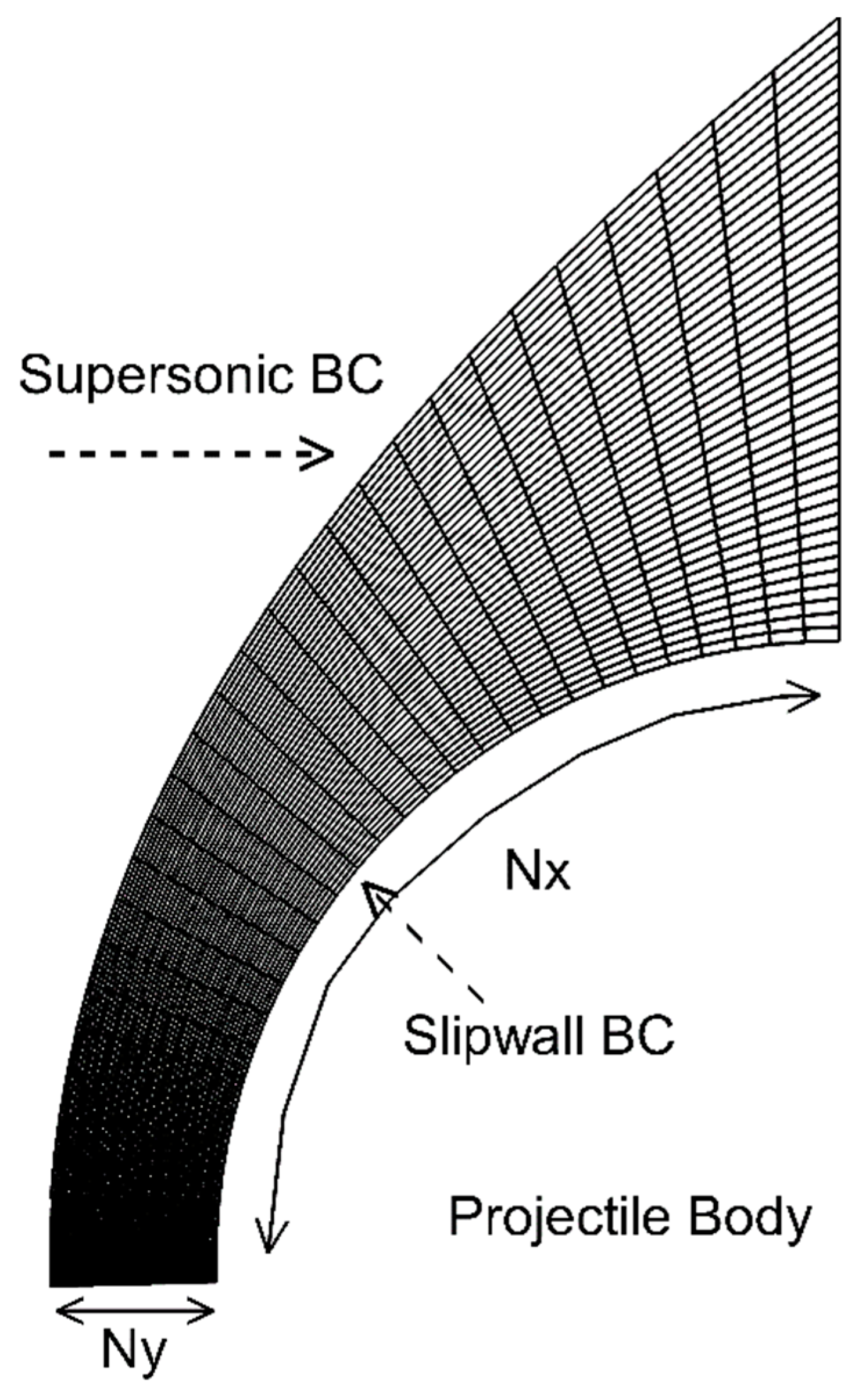
2.3. Numerical Setup

For the numerical simulation, unsteady SIC from Lehr’s experiment [7] is considered in which a hemispherical projectile of diameter 15 mm is fired into the stochiometric hydrogen–air mixture at 320 mmHg and 403 m/s of sonic velocity. The sonic velocity corresponds to the initial temperature of around 293 K. An experimental case of M 4.48 [7] is considered in the study as the flow region has sufficient induction length and the reaction zone is not too close to the projectile as seen with other cases. The inflow boundary condition is fixed to the supersonic inflow and the slip wall boundary condition is applied to the projectile surface. The far-field variables are simply extrapolated from the neighboring cells. Choi et al. [17,18] reported that grid systems comprising 150 × 200 grid points are sufficient to calculate the flow features of the SIC in which 150 points spread along the flow direction and 200 grid points spread along the stagnation streamline, perpendicular to the projectile surface. In this study, four different types of grid systems were used such as 150 × 200, 200 × 300, 300 × 450, and 400 × 600. The time step for each iteration is calculated from the fixed Courant–Friedrichs–Lewy (CFL) number and the minimum spatial resolution of the grid systems. To preserve the stability of the solution, the number is set to 0.2 for all the cases.

3. Numerical Simulation of Shock-Induced Combustion Using Different Chemical Kinetic Mechanisms

3.1. Hydrogen–Air Combustion Mechanisms

Various hydrogen reaction mechanisms are proposed around the world and all the models are validated with the experimental results; still, there are some uncertainties in the models in predicting the combustion flow field over a wide range of conditions. Chemical kinetics plays an important role in the dynamics of the combustion systems, especially for supersonic combustions where the chemical time scale is in the order of microseconds. Olm et al. [23] compared various hydrogen reaction mechanisms that were reported in the previous decade and quantitively compared the performance of the reaction models with the experimental results, such as ignition delays from shock tubes and rapid compression machines, species concentration in flow reactors and jet stirred reactors, and flame velocity measurements. In their study, they have ranked the reaction mechanism based on the model prediction with that of the experimental results. Similarly, Ströhle [24] compared the selective kinetics models for gas turbine combustion and compared the performance of the models at various conditions; however, comparing the performance of the reaction mechanisms at critical conditions, such as high pressure and high temperature, which are relevant to the experimental results, is a challenging task due to the lack of experimental data.
A preliminary study of the reaction mechanisms is conducted for their prediction of properties, such as ignition delay times and laminar flame speed. For this analysis, 10 different reaction models are considered, with a mix of widely known old chemical models as well as recently developed reaction mechanisms with high-temperature and pressure-dependent kinetics. The reaction mechanisms include, along with Jachimowski reaction mechanisms, GRI mech 3.0 [25] and Maas–Warnatz mechanism [26] as they were widely used in the early 1990s for various combustion applications. Conaire [27] and Li [28] reaction mechanisms were reported to predict the combustion flow field quite well and, hence, they were also considered. REDRAM (REDuced Ram accelerator mechanism) [29] is included as it was developed mainly for ram accelerator applications and was reported to predict the combustion regimes of RAM accelerator mixtures and conditions quite well. Dryer mechanism [30] was modeled for high-pressure applications and, hence, that was also included in the study. Finally, reaction mechanisms from the kinetics research group of the University of South California (USC) [31] and the University of California San Diego (UCSD) [32] are considered as they provide a regular update to their reaction models.

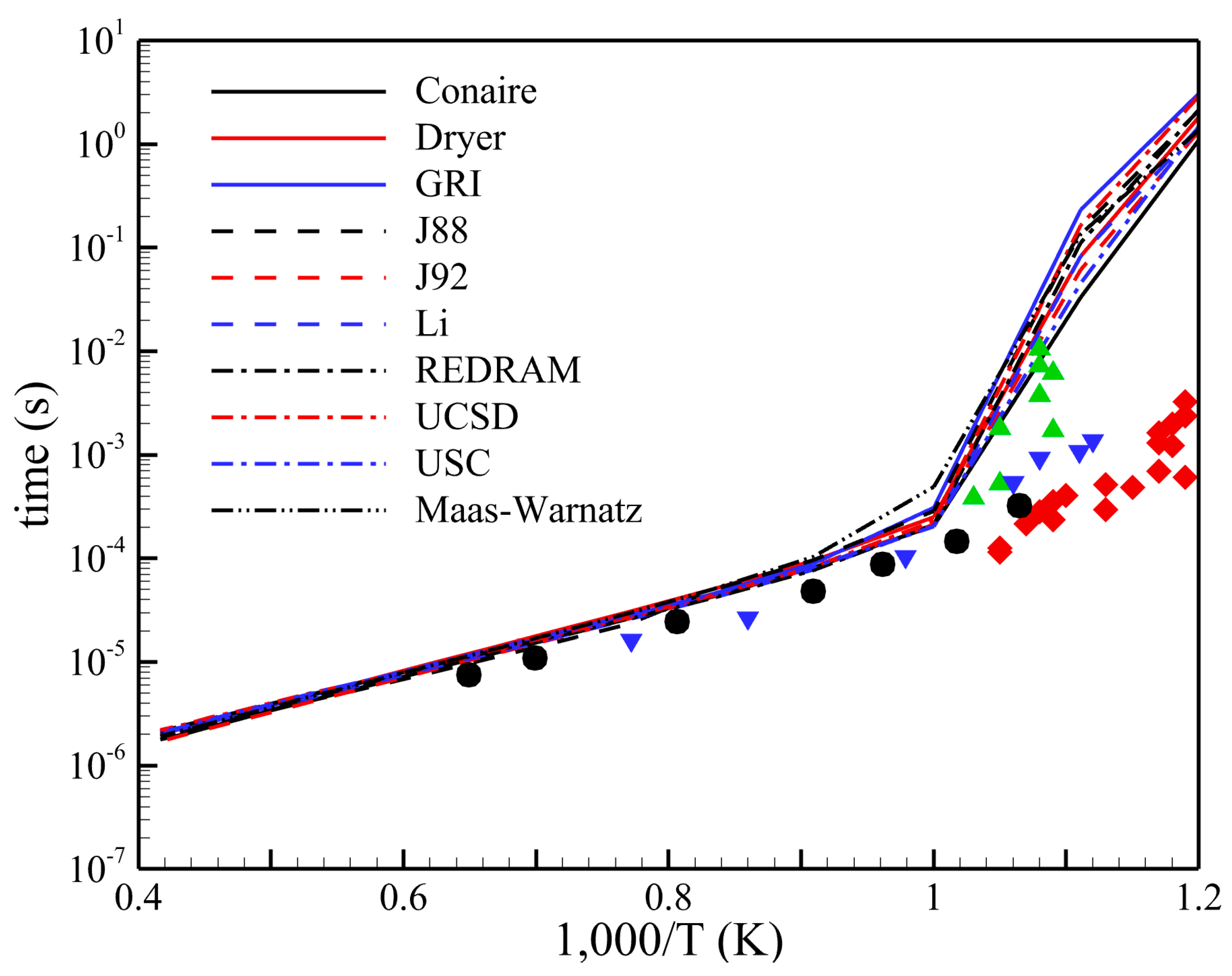
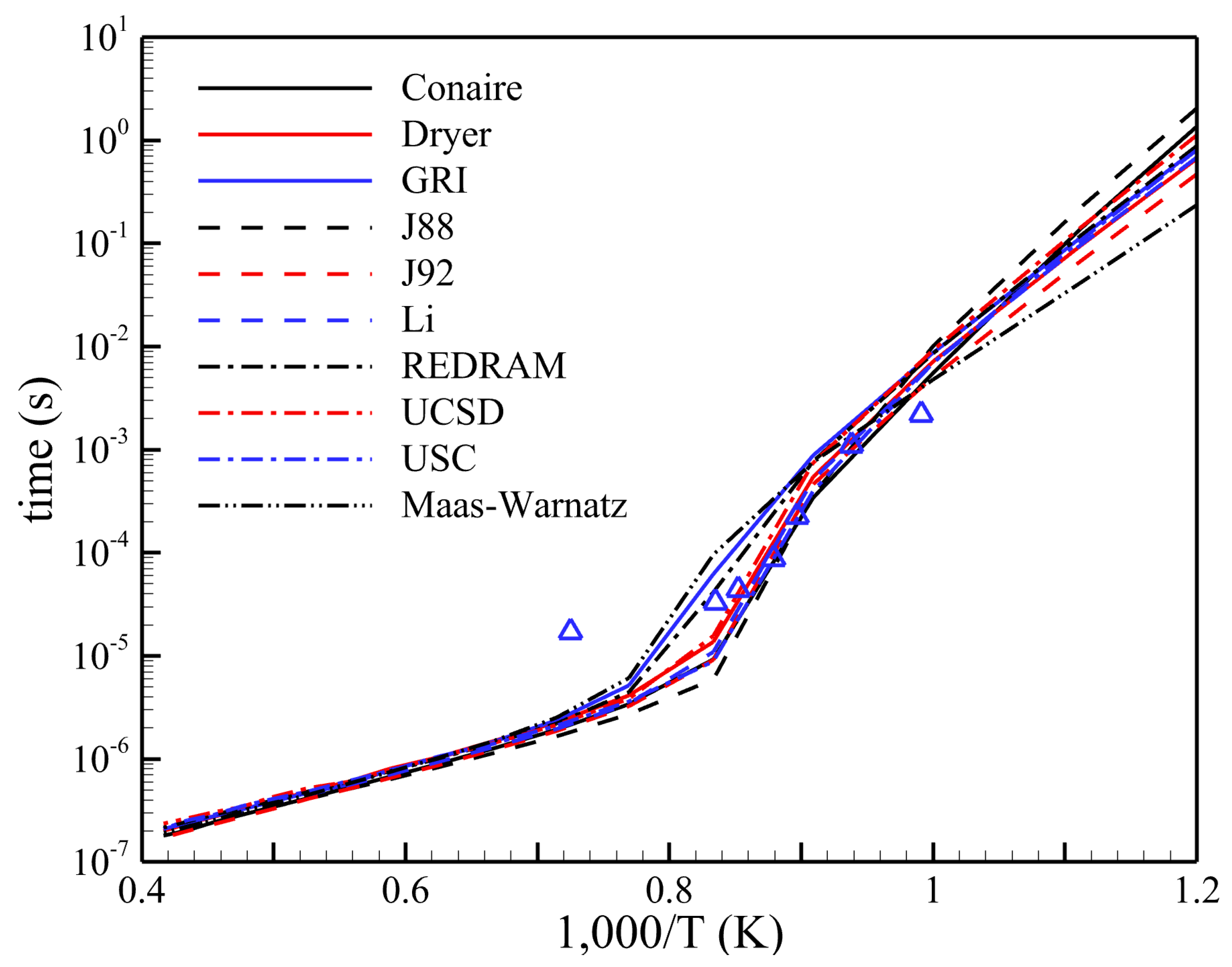
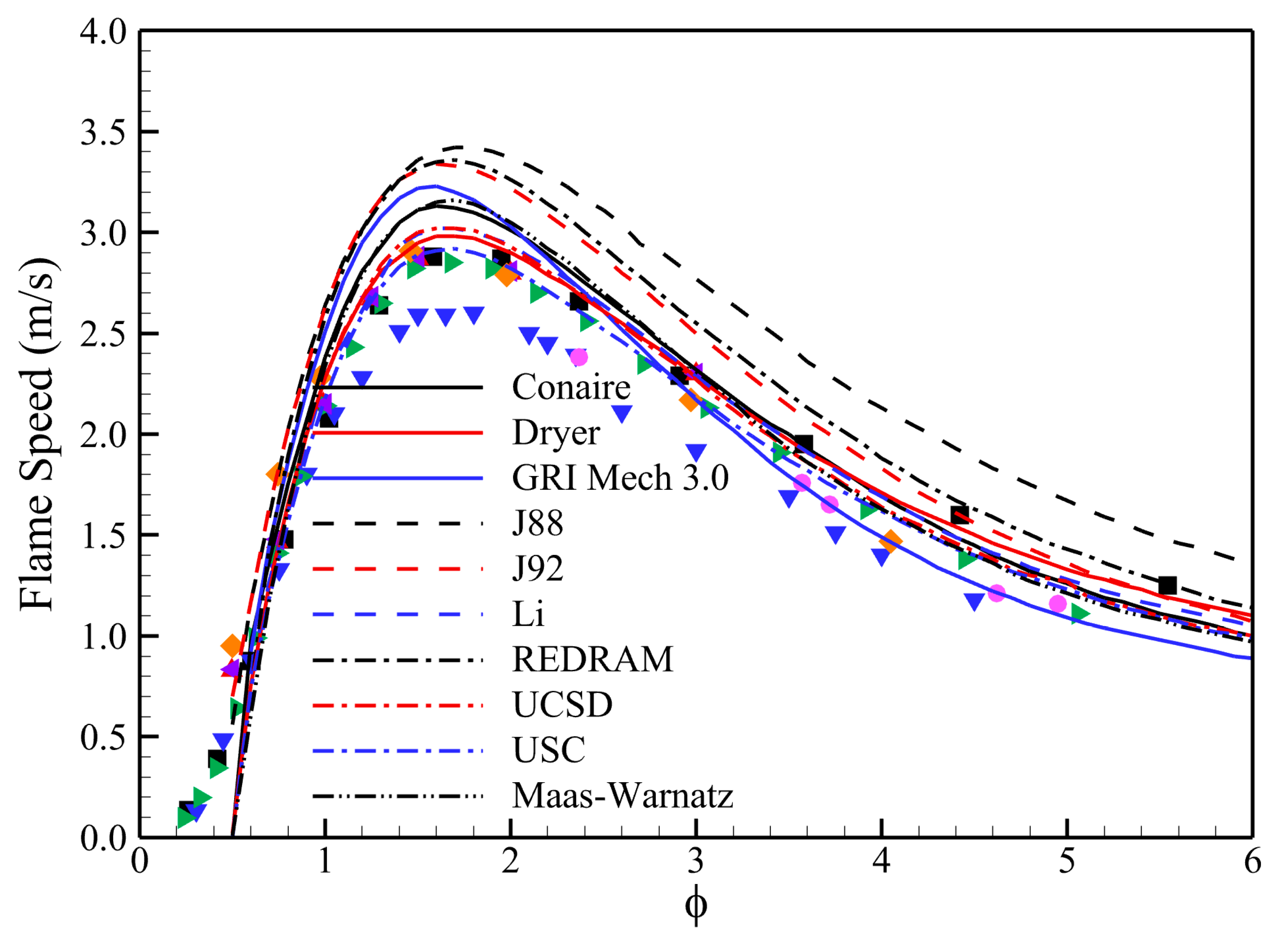
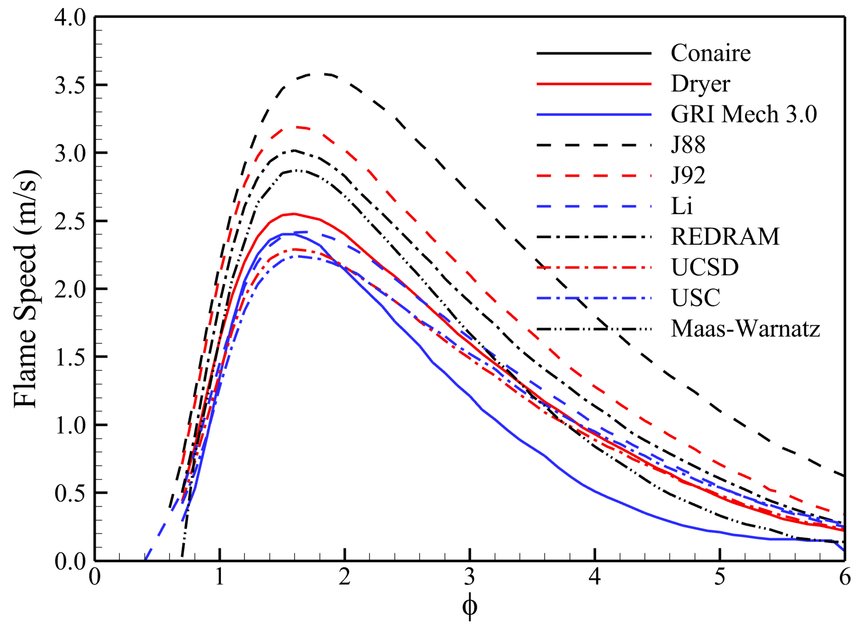
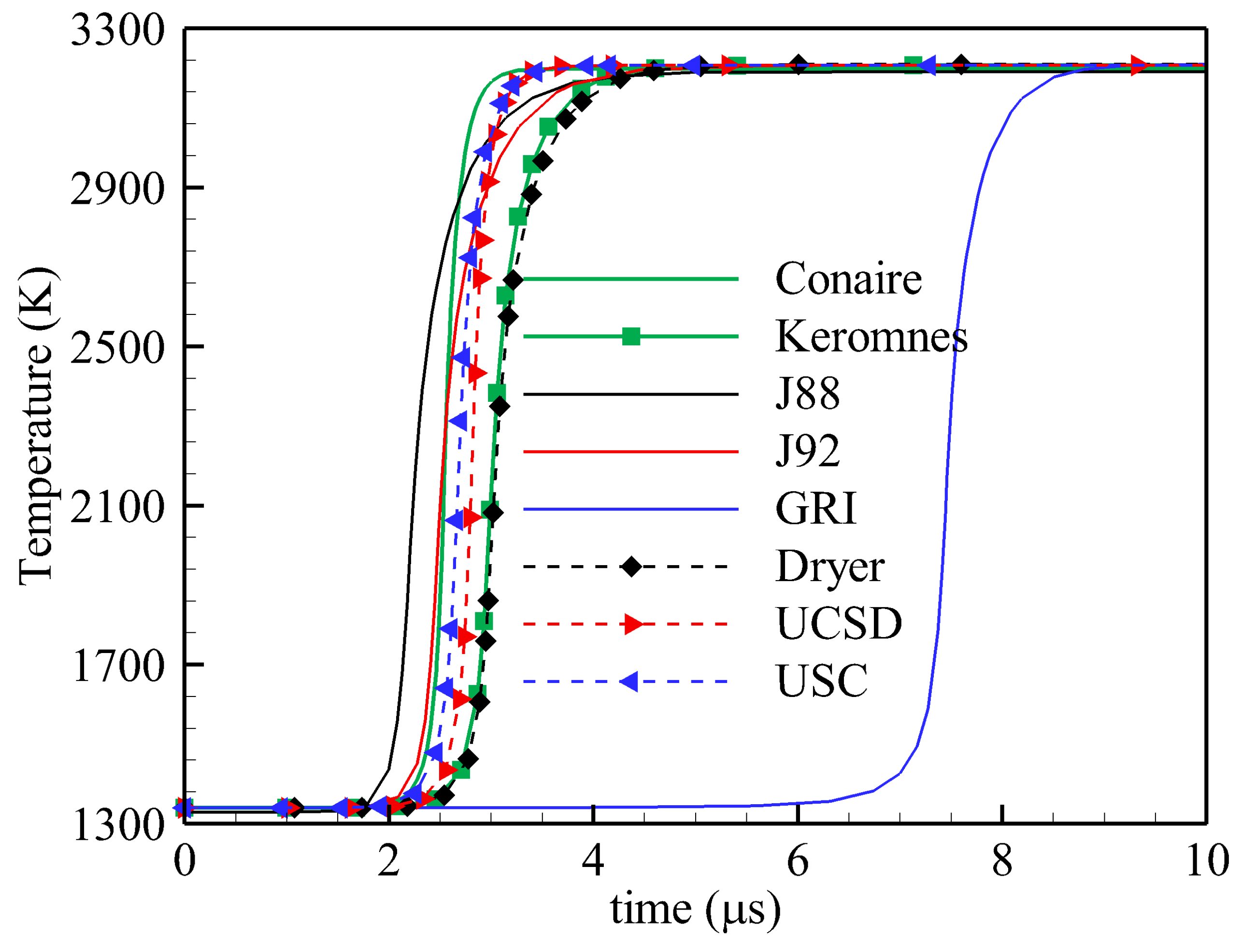
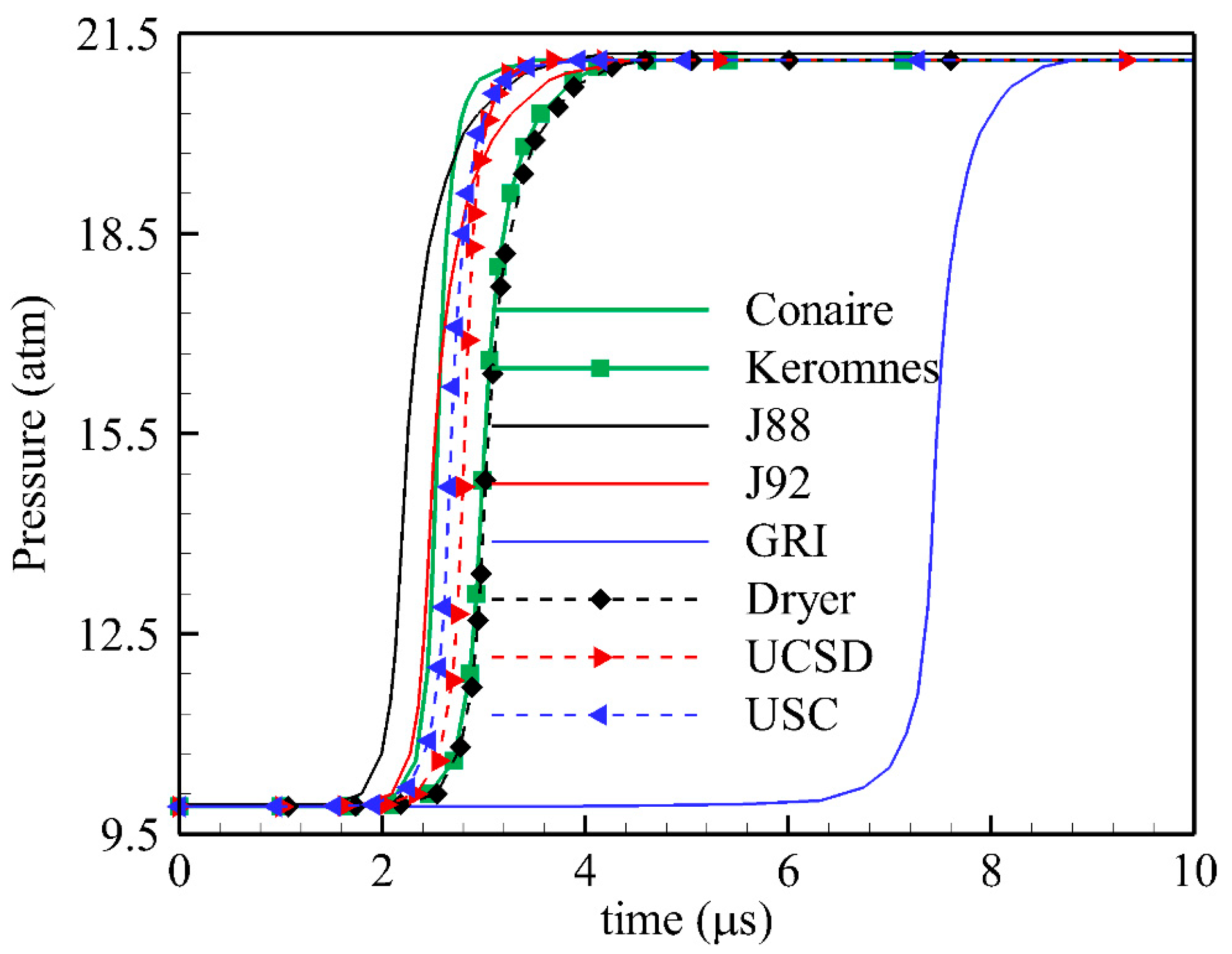
3.2. Comparison of Ignition Delay Time and Laminar Flame Speed

The present part is an extension of validation studies for the hydrogen combustion mechanisms [22]. The detailed kinetics of hydrocarbon mechanisms of the selected models are reduced to hydrogen–air reaction mechanisms using MECHMOD [33] code. The Chemkin II package was used to calculate the basic properties of the reaction mechanisms, such as ignition delay times and premixed laminar flame speed. Experimental results were taken from the ReSpecTh repository [34]. From the ignition delay times analysis, as shown in Figure 3 and Figure 4, all the models predict similar results at high temperatures. At low temperatures and 1 bar conditions, the results vary significantly, sometimes in the order of 10. At high pressure all the mechanisms, except GRI, Maas–Warnatz, and REDRAM, which under-predicts, predict results similar to the experimental result in the 1000–1250 K range. Due to limited experimental data at high-pressure conditions, validating those mechanisms is a challenging task, especially in low-temperature regions (less than 1000 K). Similarly, premixed laminar flame speed is calculated using PREMIX code from the Chemkin package and is shown in Figure 5 and Figure 6 for 1 and 10 bar, respectively. All the mechanisms predict closer to each other at stochiometric conditions but predict differently at rich mixture conditions at 1 bar condition; however, for high-pressure cases, there is a significant difference in the results, even at stoichiometric conditions. Old reaction models, such as Jachimowski and Maas–Warnatz mechanism, always over-predict the results at both atmospheric and high-pressure conditions. GRI mechanism which over-predicts the results at atmospheric pressure, predicts low flame velocity at high-pressure conditions. Due to uncertainties in the experimental results, the efficacy of quantifying the model results is also disputed. It is both arduous and numerically expensive to compare all the mechanisms for the combustion flow field. Very limited reports are available that directly compare the chemical kinetics mechanisms for combustion applications; hence, in this study, the performance of reaction mechanisms is compared directly for SIC applications.
From the preliminary analysis, six models are selected for the analysis of SIC applications, which are Jachimowski models (1988, 1992), GRI Mech 3.0, Dryer mechanism, USC mechanism, and UCSD mechanism. A constant volume (CV) explosion model [35] is used for the initial assessment of the reaction mechanisms at the initial condition of the unsteady SIC experiment. For comparative study, Kéromnès [36] and Conaire mechanism [27], which were reported to quantitively predict the experimental results better in [23], are used to understand the similarities and differences with other reaction mechanisms. The temperature and pressure variation over time is shown in Figure 7 and Figure 8. From the results, it can be seen that the older Jachimowski reaction mechanisms react earlier than the other models while GRI mechanism reacts much slower than the other models. Dryer’s mechanism predicts the reaction profile closer to that of the Kéromnès model for this case. UCSD and USC reaction mechanisms predict results between the Conaire and Kéromnès mechanisms. The ignition delay, calculated at the time when maximum temperature gradient occurs, for all the reaction mechanisms is tabled in Table 1. All the reaction mechanisms predict similar ignition delays other than GRI mechanism which under-predicts, and Jachimowski-88 reaction mechanism which over-predicts the result compared to the other mechanisms. The difference between the rest of the mechanisms is in the order of a few tenths of μs.

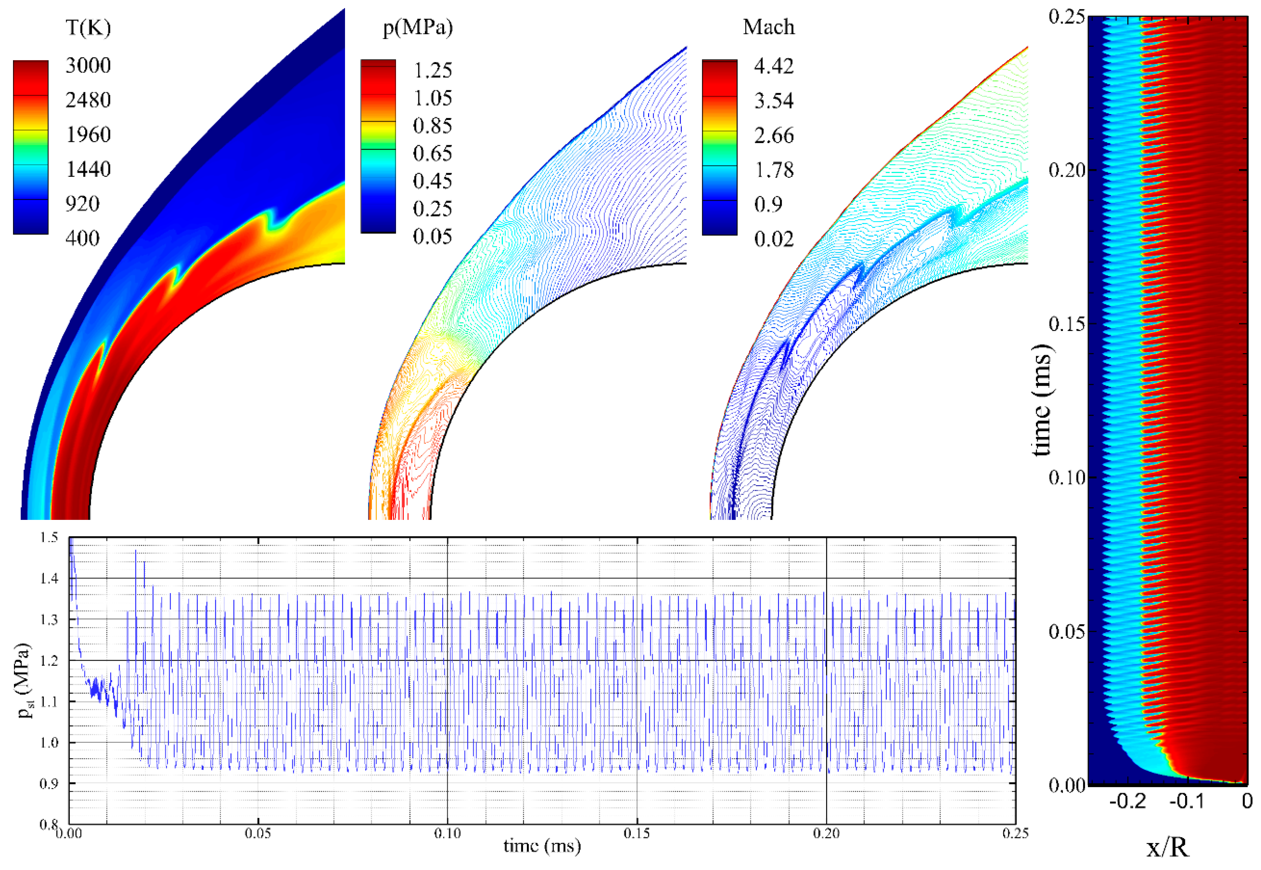
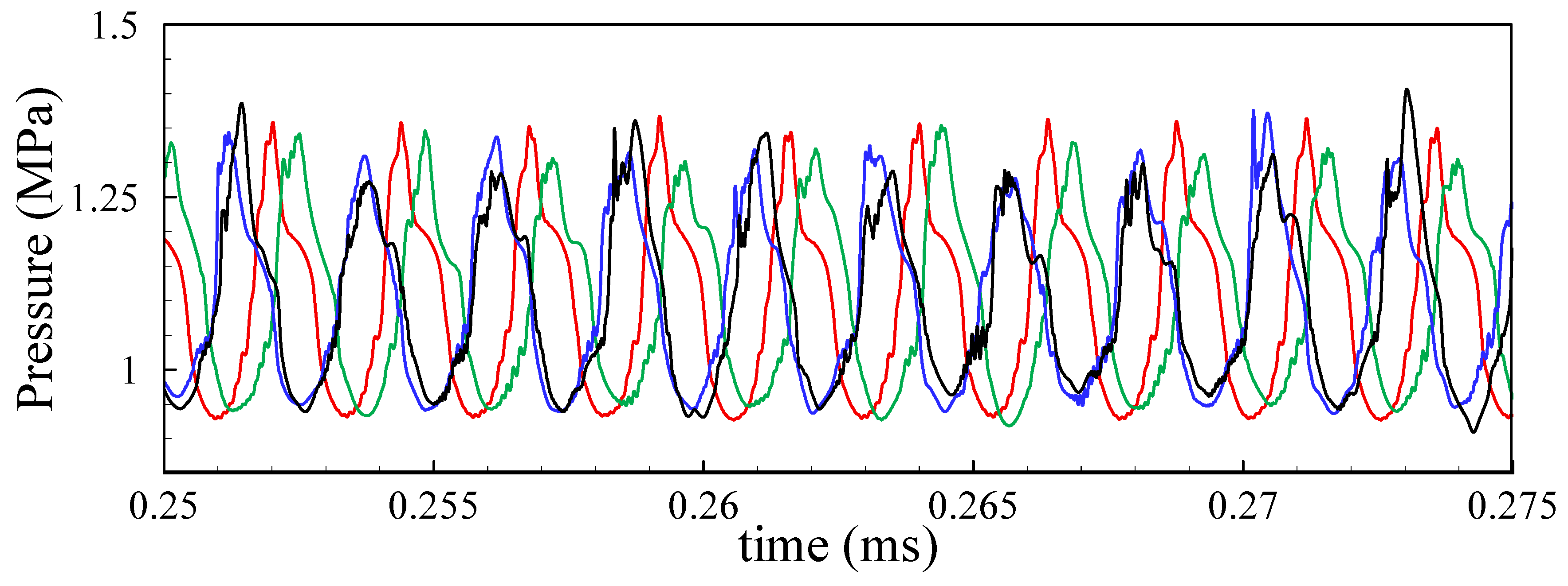
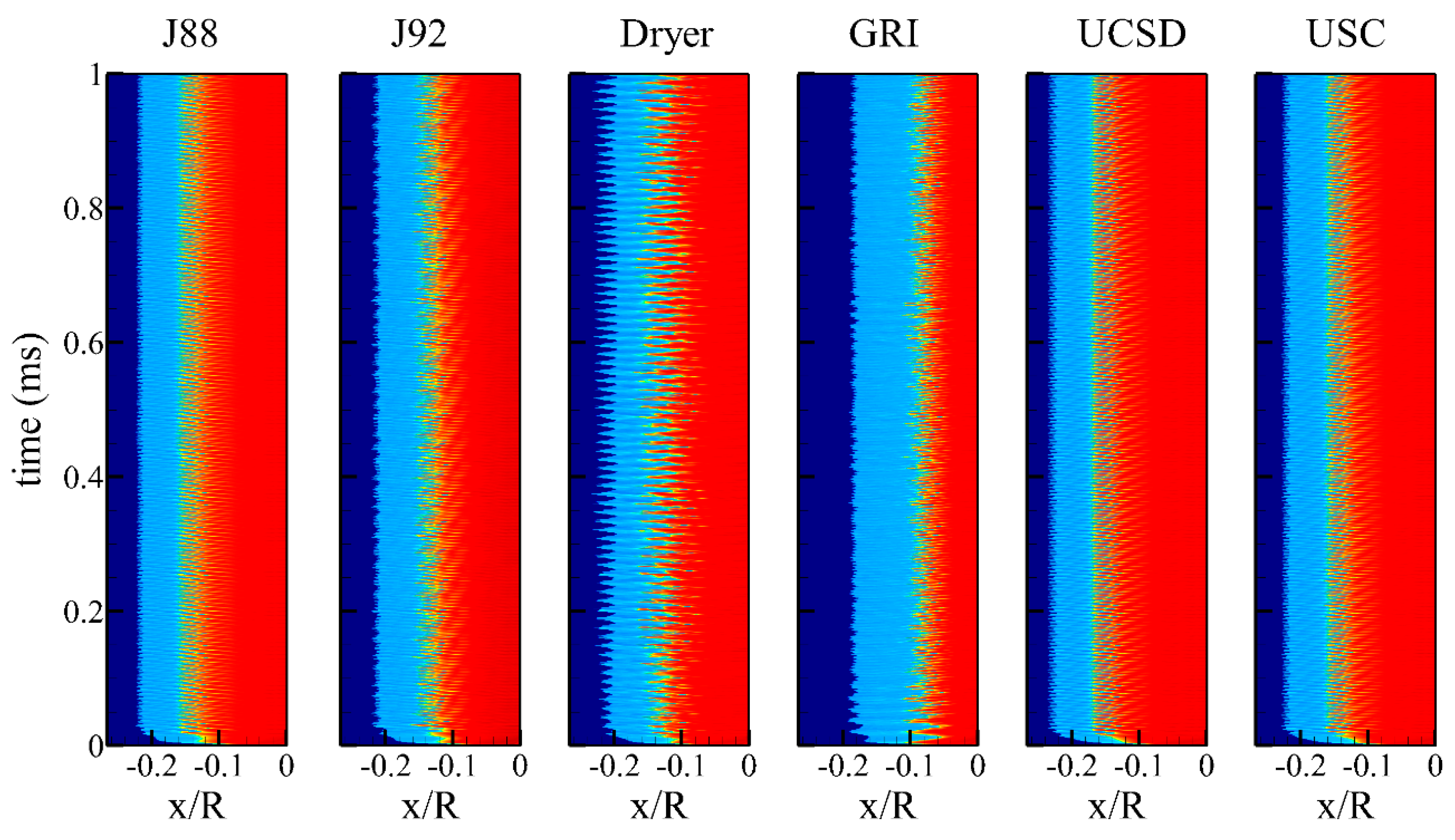
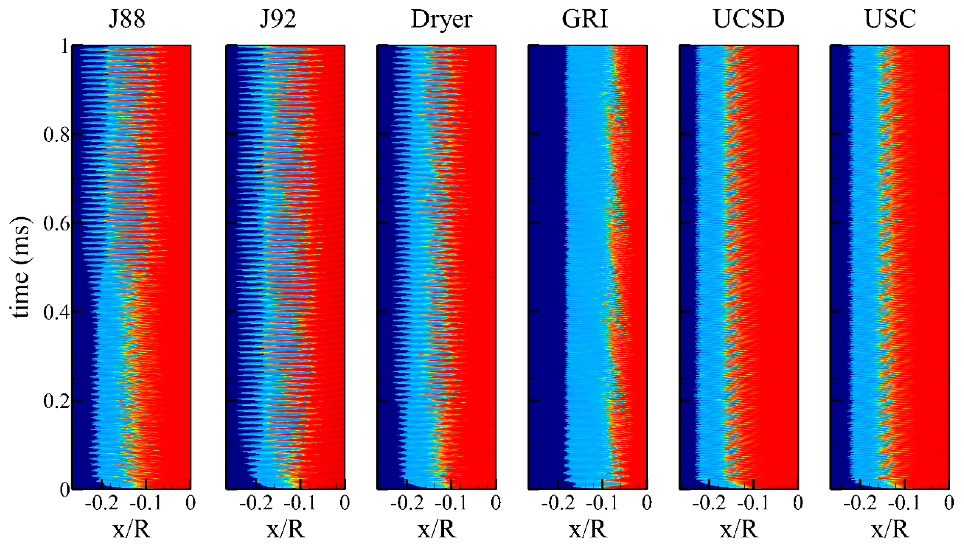
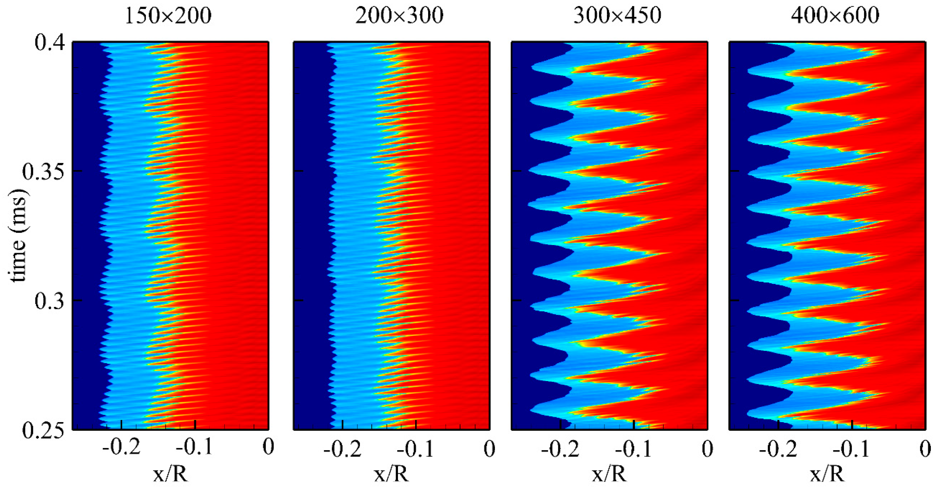
3.3. Comparison of the Mechanisms for SIC Flow Field

An overview of the results with instantaneous temperature, pressure, and Mach contour for Jachimowski-88 mechanism with 150 × 200 is shown in Figure 9. The instantaneous plots clearly illustrate the regularity of the independent cycles of oscillation. The compression waves being reflected from the projectile surface are also clearly shown in the pressure contour. The interaction of the reflected compression wave and the reaction zone creates a new cycle and this process causes the oscillation in the flow field. A pressure probe is attached at the stagnation point of the projectile and pressure is extracted over time for all the iterations, as shown in Figure 9. FFT analysis of the pressure variable shows the oscillation frequency of the flow field. Also, an x-t graph, which contains the flow variations along the stagnation streamline, is created in the direction normal to the flow and is shown in the same figure. From these figures, it is evident that the resulting fluctuations are very regular.
The pressure graph probed at the stagnation point for all the grid systems systems with UCSD reaction mechanism is shown in Figure 10. The flow field exhibits slight disturbances at high grid resolution in the peaks, however, the disturbances do not affect the periodicity of the oscillation. The flow field around the projectiles for various reaction mechanisms with 300 × 450 grid system is shown in Figure 11. Jachimowski-92 and Dryer mechanism predicted results closer to the experimental results at coarse grid resolution considered in the study; however, with a slight increase in grid resolution, the models predict spurious oscillation which resulted in a low-frequency instability phenomenon. As seen from the Mach contour in Figure 11, the periodicity of the oscillation is affected which, in turn, affects the dynamic of the flow field. The GRI mechanism could not capture the induction zone adequately, which resulted in an unphysical low-frequency oscillation. This reflects the sensitivity of the chemical mechanisms to grid resolutions at high-temperature conditions.
Similarly, high-fidelity simulations were performed for all the reaction mechanisms at all grid levels. Figure 12 and Figure 13 show the x-t graph depicting the evolution of the SIC flow along the stagnation streamline for all the reaction mechanisms at the base grid and fine grid resolutions. In the following x-t diagrams, the temperature legend is the same as Figure 9. All the reaction mechanisms, except Jachimowski-92 and GRI mechanisms, produce a regular oscillation at base grid resolution. Firstly, GRI mechanism predicts low ignition delay times from the CV explosion model for this initial condition. As a result, the resulting flow field predicts a longer induction zone and, hence, the resulting flow field oscillation is low when compared to the experimental frequency. With the increase in grid resolution, the reaction mechanism does not show any significant difference in the prediction and always predicts a low-frequency oscillation. Secondly, the Jachimowski-92 mechanism predicts a low-frequency oscillation along with a regular oscillation even at low grid resolution; however, with a slight increase in the grid resolution, the spurious reactions are suppressed, and the resulting flow field predicts a regular oscillation with few disturbances. With further increase in the grid resolution, the low-frequency oscillation supersedes the regular oscillation and, finally, results in a high-amplitude low-frequency oscillation. The evolution of the flow field from 0.25 ms to 0.4 ms is extracted for all the grid systems with the Jachimowski-92 mechanism, as shown in Figure 14.
The Dryer mechanism predicts a regular oscillation at base grid resolution (150 × 200), however, with a slight increase in the grid resolution, the flow field is disturbed and finally results in an unphysical oscillation. The streamline variation of the temperature contour is highlighted in Figure 15 for all the grid systems considered in this study. With further increase in the grid resolution, the flow field is not much affected and always predicts a distorted oscillating flow field with high-amplitude low-frequency oscillation. The Jachimowski-88 mechanism predicts a very regular oscillation, however, at fine grid resolutions (400 × 600), the low-frequency oscillation steadily attenuates and, finally, results in an unphysical instability phenomenon, as observed with J92 and Dryer mechanisms. The evolution of the instability phenomena is clearly observed at fine grid resolution with the Jachimowski-88 mechanism and is highlighted in Figure 16. The UCSD and USC mechanisms also exhibit sensitivity and develop disturbances at fine grid resolutions (400 × 600), but the disturbance does not convert into any instability, as seen in Figure 13. From the results of the Jachimowski-88, -92, and Dryer mechanisms, it is obvious that this artificial instability is caused by the discrepancies in the chemical kinetics rate and, also, they are grid-sensitive. These results further exemplify the role of reaction mechanisms in the analysis of combustion instability problems.
The periodicity of the SIC oscillation depends on the strength of the compression wave. In the case of the Jachimowski-92 and Dryer mechanisms, the strength of the compression wave is much stronger at high grid resolution, which results in such a low-frequency large-disturbance regime-like profile. Accurate analysis of the strength of the compression waves is essential in the case of high-speed combustion systems. Even the recently developed Dryer reaction mechanism, which was modeled explicitly for high-pressure combustion, results in a stronger compression wave and predicts a low-frequency irregular oscillation with high amplitude along with the high-frequency regular oscillation. Even though the strength of the compression wave is strengthened with an increase in the grid resolution for the USC mechanism, the flow physics remains unaltered. Similar to the UCSD mechanism, the USC mechanism also predicts the combustion well without disturbances at high grid resolutions; however, the disturbances were comparatively higher, and, hence, it is concluded that of all the reaction mechanisms considered in this study, the UCSD reaction mechanism performs best. The oscillation frequencies for all the cases calculated from the FFT analysis of the pressure probe results are listed in Table 2. From the FFT analysis, it is evident that when low-frequency instability occurs, high-frequency oscillation also exists but becomes a secondary mode of oscillation.

4. DMD Analysis of the Shock-Induced Combustion Instability

Significant advances have been achieved in the previous few years in the extraction of coherent structures from experiments and numerical simulation results. The DMD is a data-processing algorithm that extracts coherent structures with a single temporal frequency from a numerical or experimental data sequence. The data are flow field variables (snapshots) saved over a time with a fixed time interval. These snapshots contain information on both linear and nonlinear structures in the flow field. The dynamic mode decomposition enables the extraction of the main linear structures existing in a flow field that bonds the data in snapshots through a linear model. The importance of POD and DMD modes goes beyond the identification of coherent structures in fluid flows. They may be used to obtain reduced-order models by projecting the full system onto the subspace spanned by the extracted modes [37,38,39]. Modal decomposition is being used recently to investigate the combustion instability problems in supersonic combustors [40] as well as in rocket combustors [41,42]. DMD has also been applied to reacting flows. Richecoeur et al. [43] discussed the parameters influencing the quality of DMD when applied to experimental data from turbulent combustion, focusing on combustion dynamics. The DMD also has the advantage to be field-selective. The field selection is, for instance, the choice of specific two-dimensional planes in a three-dimensional space where snapshots are recorded. Both proper orthogonal decomposition (POD) and DMD are post-processing algorithms based on the instantaneous results called snapshots. While POD modes are characterized by spatial orthogonality and multi-frequential temporal content, DMD modes may be non-orthogonal, but each possesses a single temporal frequency. This lack of non-orthogonality of DMD modes may be essential to capturing significant dynamical effects in systems with non-normal dynamical generators.
The POD analysis decomposes into different modes, and the modes are ranked by the accumulated energy content of each mode [44]. The first mode has the maximum energy content, and it corresponds to the ensemble mode which is similar to a time-averaged solution. Also, the DMD analysis shows ensemble mode which is similar to the time-averaged solution around 0 kHz with a high coherence value which is used to normalize the coherence of other fluctuating modes. For the other modes, ϕ describes the level of fluctuation occurring in that cycle. The instability mechanism is observed even with 200 × 300 grid system when using the Dryer mechanism; hence, the decomposition of flow field at fine grid resolution, i.e., 400 × 600 grid system, which produces regular oscillation with the UCSD mechanism and low-frequency instability with the Dryer mechanism, is taken for further analysis.

4.1. Description of Modal Decomposition Analysis

For DMD analysis, the first step is to construct a matrix V m and V m + 1 with physical flow field variables. The column matrix v containing the physical variables are called snapshots and are taken at equal intervals of time. The matrix containing the snapshots is stored as shown below:
V m = [ v 1 , v 2 , , v m ]   and   V m + 1 = [ v 1 , v 2 , , v m ]
The matrices V m and V m + 1 have rows containing the scalar data of the physical variable and columns corresponding to the number of snapshots considered for the analysis. There exists a theoretical matrix between the snapshots which contains the nonlinear bond that exists between the snapshots and is expressed as:
V m + 1 = A V m
The DMD aims to compute this theoretical matrix from which the temporal and spatial characteristics of the flow field are studied. Singular value decomposition is first computed out of the matrix V m
SVD   ( V m ) = U W H
Here, U and W are the orthonormal matrices with dimension ( n , n ) and ( m , m ) . The matrix has dimension ( n , m ) with its quadratic part having diagonal matrix of size ( m , m ) . The symbol H represents the Hermitian operator and the matrix can be rearranged to compute the theoretical matrix A as follows:
V m + 1 = A U W H
The above equation is valid in space n and can be reduced to space m . In order to do that, ( n , m ) is replaced with m ( m , m ) and U ( n , n ) is replaced with U m ( n , m ) . From this reduction, the equation can be rearranged as:
V m + 1 W m 1 = A U m
Both sides are multiplied by the Hermitian of the matrix U m to obtain the following:
U m H V m + 1 W m 1 = U m H A U m
From the above equation, the approximate of the theoretical matrix A can be obtained. To obtain the linear solution to this problem, an eigen decomposition is performed on the approximate of the theoretical matrix which results in the following.
U m H A U m Z i = λ i Z i   or
U m H V m + 1 W m 1 Z i = λ i Z i
where λ i and Z i are the ith eigenvalue and eigenvector of the projected matrix. The pseudo eigenvector of the matrix E i D M D are then computed by multiplying the matrix U m with the eigenvector Z i which is expressed as
A U m Z i = λ i U m Z i
A E i D M D = λ i E i D M D
The oscillating frequency f i and the temporal characteristics such as growth rate ξ i of each decomposed mode is calculated from its corresponding eigenvalue λ i as follows:
A r g ( λ i ) = 2 π f i Δ t + 2 π p
ξ i = ln | λ i | Δ t
The growth rate provides information on whether the oscillatory mode is growing or attenuating. If the value is positive for a given mode, the amplitude will grow and the oscillation will grow. The negative growth rate signifies that the amplitude of the mode will decrease and its amplitude will decay as time goes on.

4.2. Time-Sequencing of the Snapshots

Time-sequencing in recording the snapshots is essential in capturing the essentials of the decomposed modes. In this study, the snapshots are recorded in such a way that at least five cycles of oscillations are recorded in any calculation. For example, consider that the flow oscillates at 5 Hz and 50 Hz. The flow field contains low-frequency x and high-frequency 10×. Both must be recorded. The high frequency suggests the time difference between each snapshot (1/10× = 1/50 > 0.02 s). Low frequencies suggest the total screening window and have five cycles of oscillation, and we should consider five times the low-frequency time. The time for one oscillation to be recorded is 1/5 = 0.2 s. To record five oscillations, we should consider 1 s with time-sequencing of the snapshots in the order of 0.02 s. The total number of snapshots and the time interval between each snapshot are fixed based on the FFT results so that both the high-frequency and low-frequency modes can be extracted.

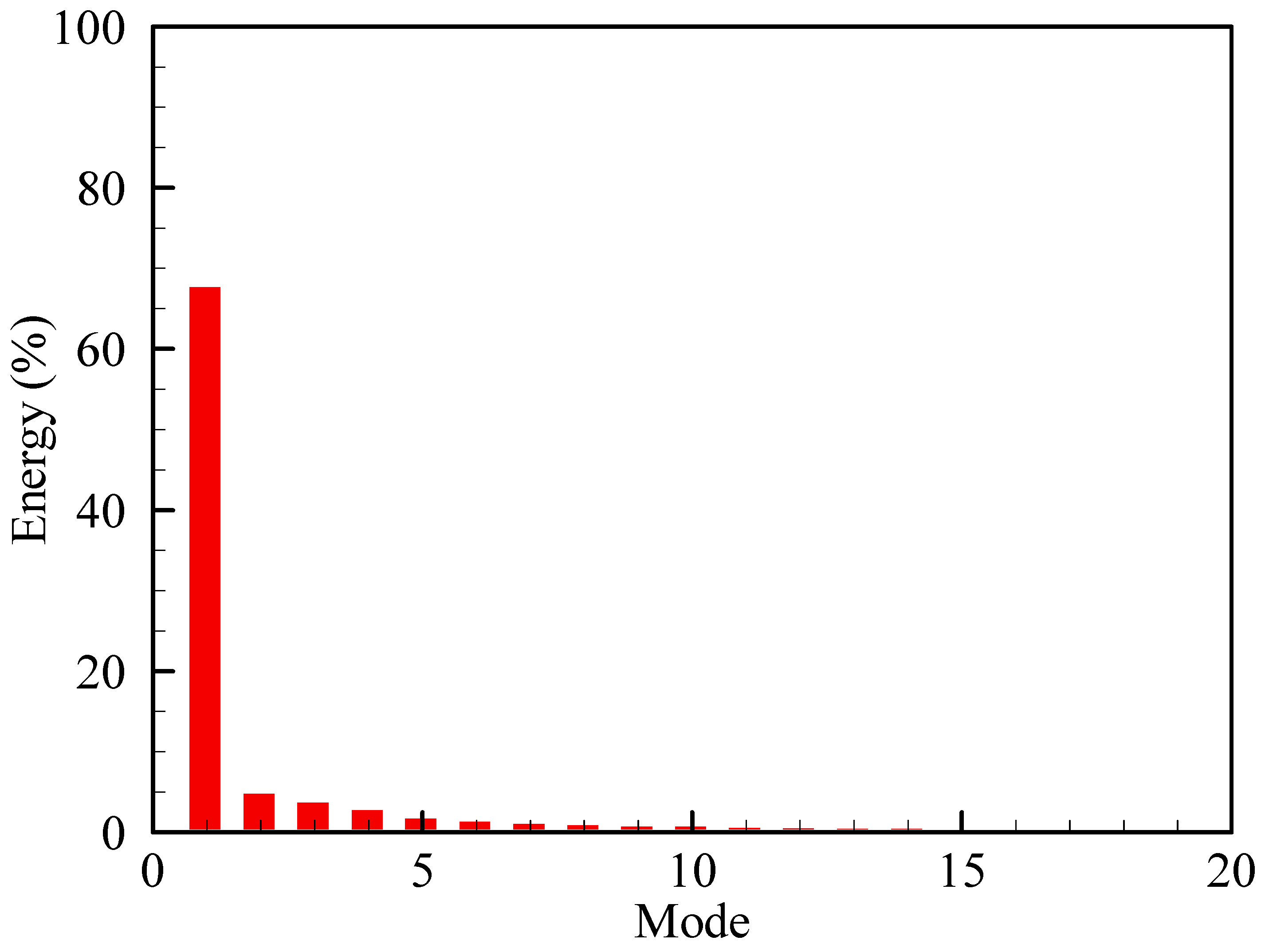
4.3. Ranking of the Modes

Coherence is used as a parameter to rank the modes as considered by Schmid [45] in his original DMD formulation. This is done by first calculating a matrix G
G = V 1 N 1 1 Y
where V 1 N 1 represents the first N snapshots, 1 is calculated from the SVD operation of the projected matrix [A], and Y represents the eigenmodes of the projected matrix. Finally, coherence is calculated from each column g i of the matrix G
E i = g i 1
The value of coherence of each mode is normalized with the mean mode to analyze the contribution of each mode to the flow field while the damping coefficient produces information on whether the mode is stable or not; however, because of the large number of modes considered for analyzing the low-frequency modes along with the high-frequency modes, reverbed modes are also observed along with the coherent modes. The advantage of using the DMD method is that each coherent structure was mapped to its temporal characteristics which is the fluctuating frequency, but ranking the decomposed modes in DMD is complex and not as reliable as the POD ranking method; hence, the coherent structures were extracted first and compared with the POD modes. To analyze the spatial structure of the primary mode, the coherent spatial structure of the POD mode is also analyzed and compared with the DMD modes for further analysis. The temporal characteristics of the DMD modes with the UCSD mechanism with 200 × 300 grid system are shown in Figure 17. Additional modes can also be seen along the primary modes around 400 kHz with high coherence values. The normalized energy content of the POD analysis for the same snapshots is shown in Figure 18. The spatial structure of the primary modes in both the POD and DMD analysis resembles the same as shown in Figure 19. Figure 19, Figure 20, Figure 21, Figure 22, Figure 23 and Figure 24 are normalized figures between red and blue. Red extreme represents one mode of negative oscillation while blue represents positive mode of oscillation; thus, along with the coherence value, POD analysis is also considered and compared to analyze the spatial coherent structure of the fluctuating flow field.

4.4. Modal Decomposition of the Flow Field with Regular Oscillation

Temporal characteristics along with the spatial coherent structures of dominant modes for regularly oscillating flow field with the UCSD mechanism are shown in Figure 20. The temporal characteristics show a dominant mode (primary mode) oscillating at 419.29 kHz which is also comparatively more stable than the other fluctuating modes. The other dominant mode is at 841.9 kHz which has a higher coherence mode and relatively weaker stability than the primary mode. The spatial coherent structure shows the reverbed mode of the primary oscillating mode. Another interesting mode observed within this selected stability window is the low-frequency mode oscillating mode 70 kHz. The spatial structure of the mode shows that the impact of this mode is in the reaction zone of the flow field; however, the dominance of this mode is less as the coherence value is comparatively too low for the analysis. POD modes of the same snapshots are shown in Figure 21 and, as can be seen, the primary modes show a similar coherent structure to that of the primary DMD mode. The coherent structures of the other modes with high energy content can be seen but they include structures of multi-frequency modes as they are not mapped based on their temporal characteristics. From the spatial structure of the primary mode, the impact of the oscillation is seen around the reaction zone where new additional reaction zones are formed as observed in the numerical results, and other regions around the projectile surface where the compression waves from the reaction zone are reflected; thus, the two processes happen at the same frequency and dictate the periodicity of the oscillating flow field.

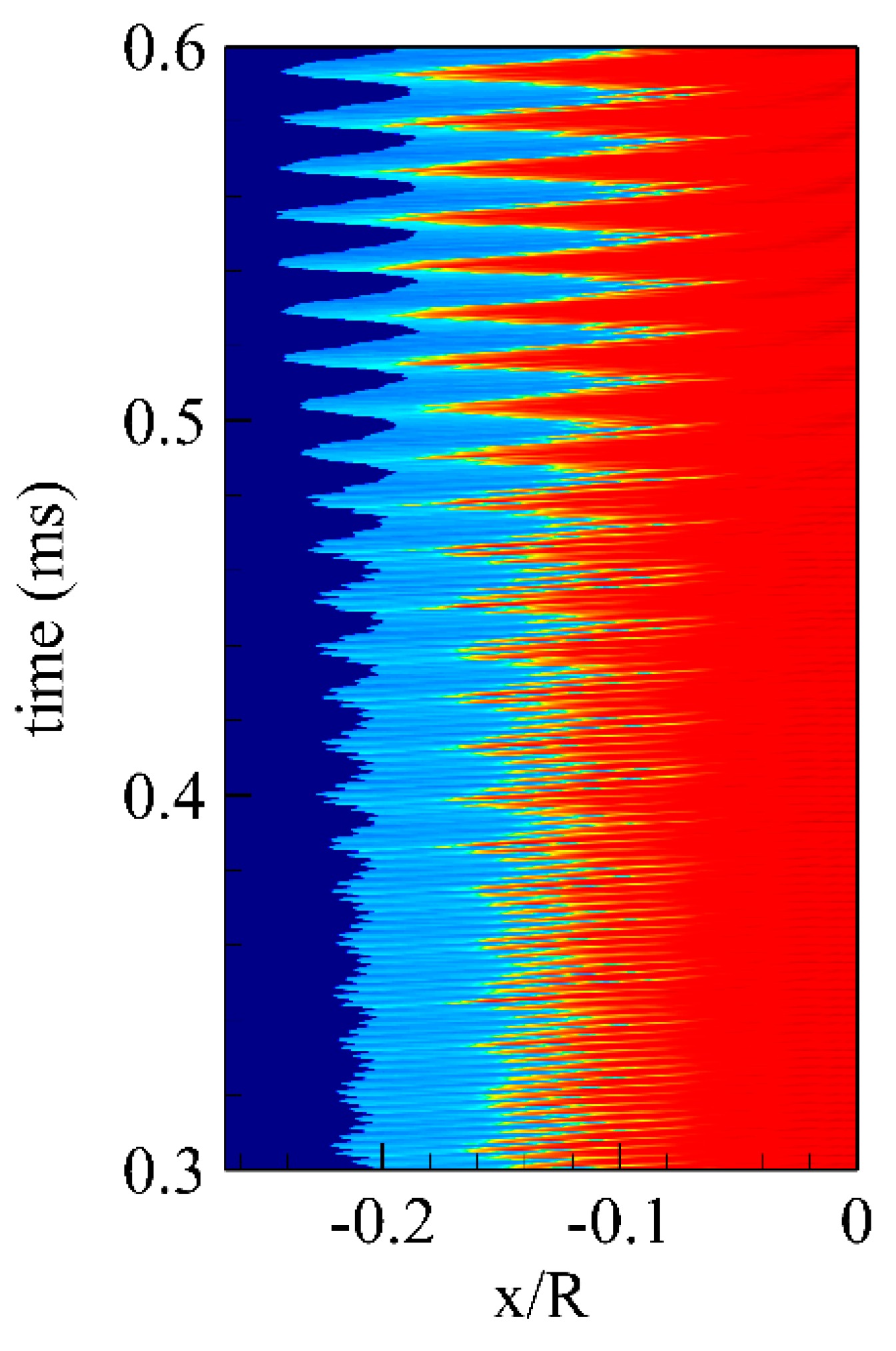
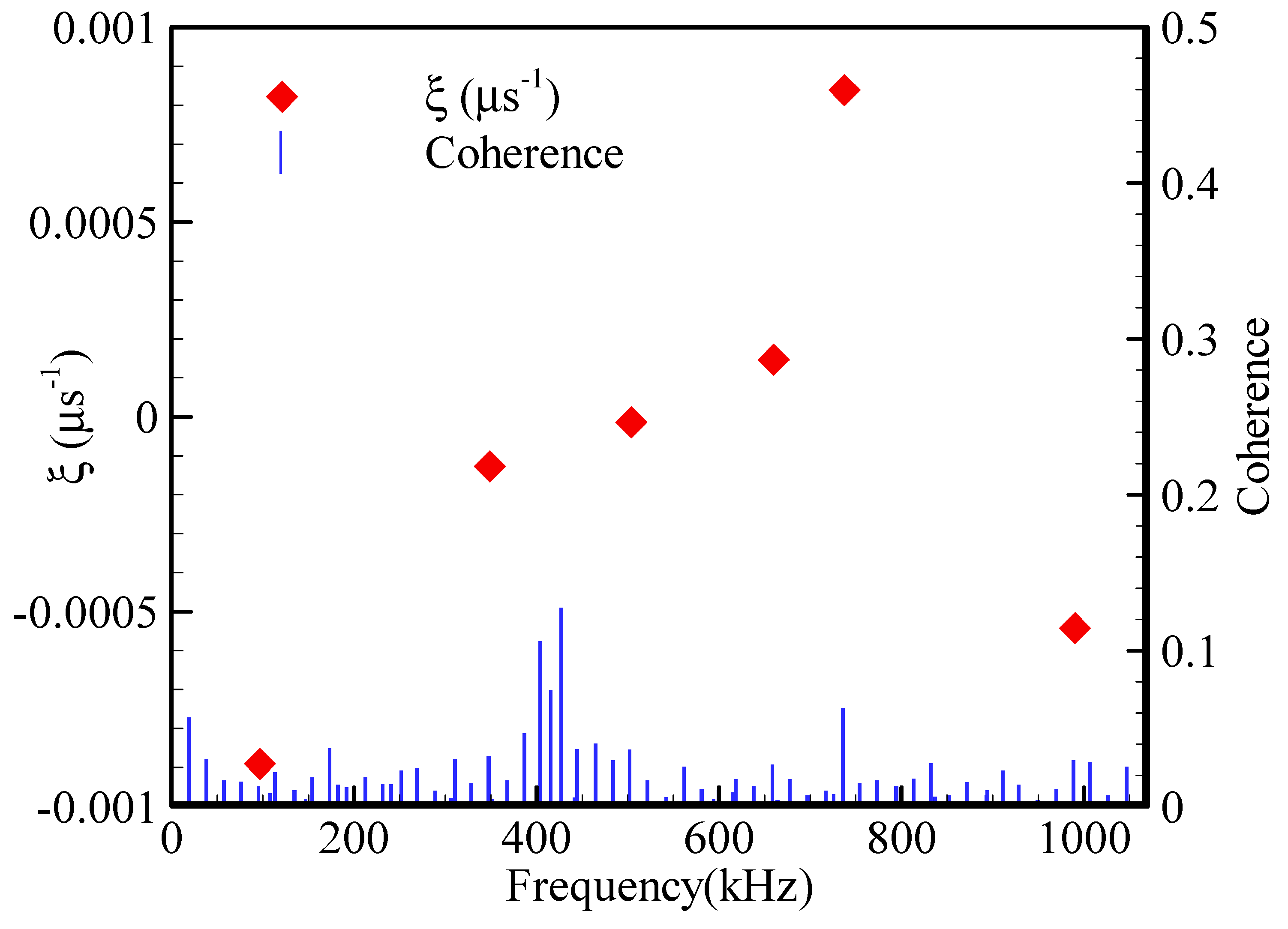
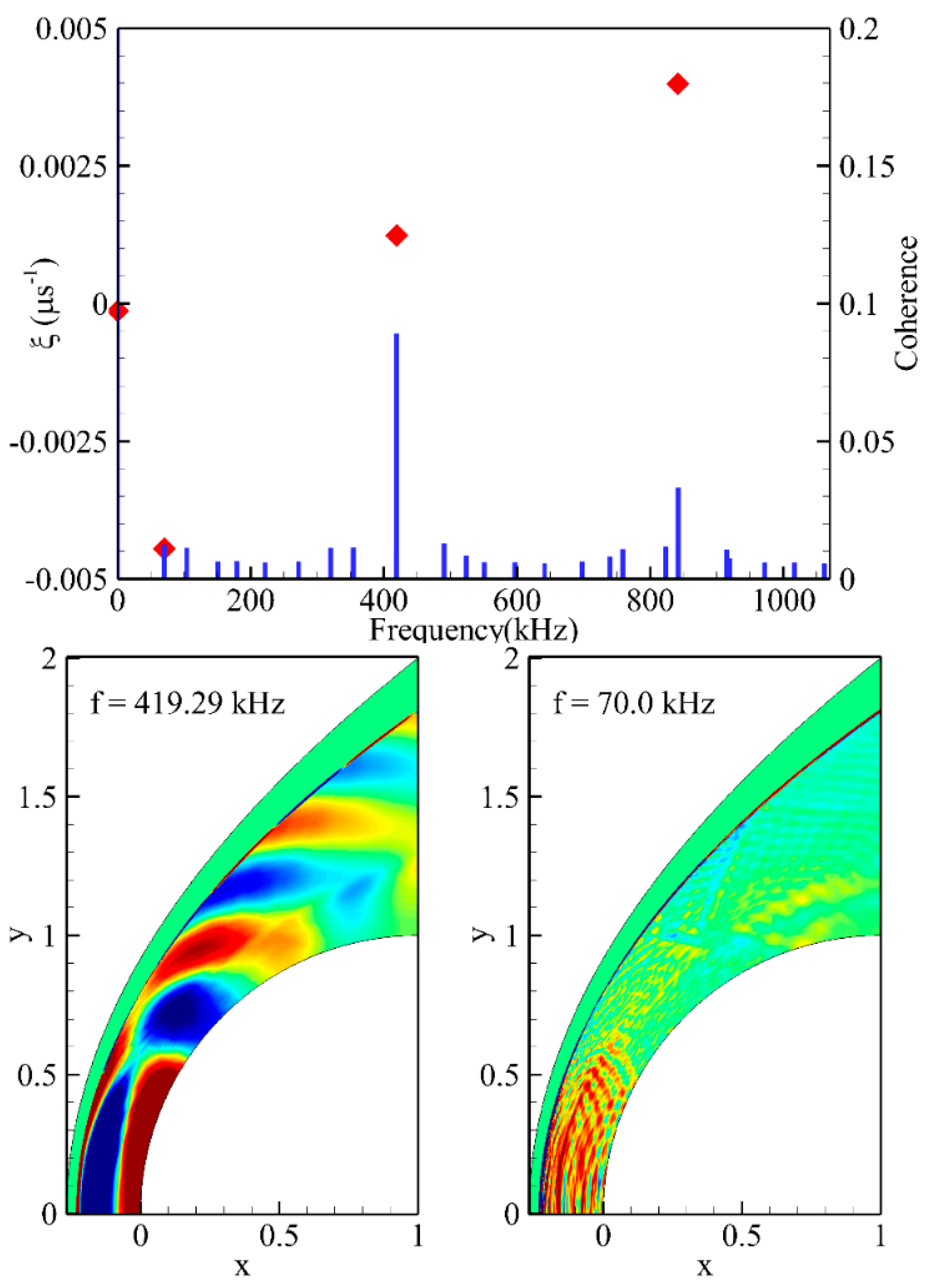
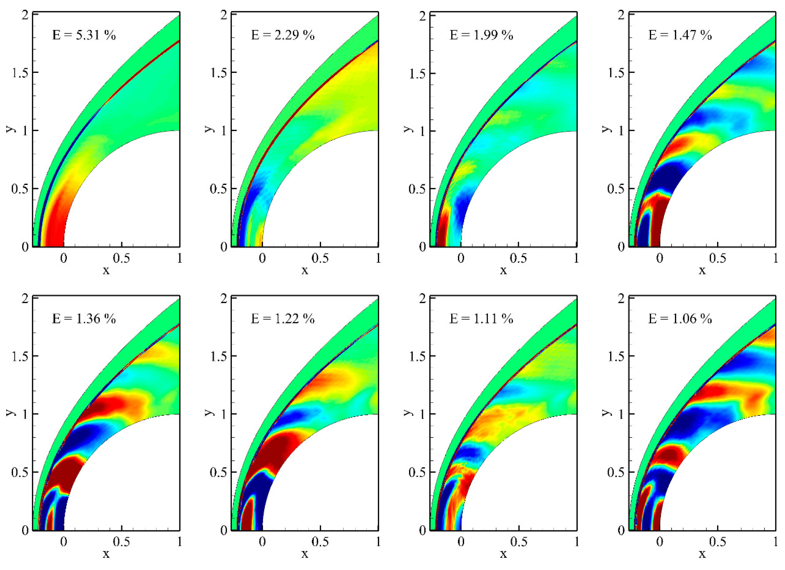
4.5. Modal Decomposition of the Flow Field with Instability Phenomena

Temporal characteristics and the spatial coherent structures of the decomposed modes of the oscillating flow field with the Dryer mechanism are shown in Figure 22. From the coherence value, it can be seen that the dominating flow field is shown at 76.8 kHz. POD analysis of the same flow field with the same snapshots is shown in Figure 23 which confirms the dominant spatial structure of the low-frequency mode with 5.31% energy content. The second dominating mode, which has a frequency of around 152.4 kHz, shows a similar spatial structure with an energy content of around 2.29% which is the effect of the dominating mode. The dominating mode is stronger in the reaction zone of the flow field while the effect can be seen in the second next dominating mode with additional fluctuations behind the shock wave. Upon analyzing the spatial structure of the modes with frequency around the experimental value, it can be seen that the coupled mechanism, oscillations around the reaction zone, and the reflecting compression waves that were observed with the UCSD mechanism were decoupled. The temporal characteristics of the experimental mode, which is 459.8 kHz, show a lower coherence value and more stable damping coefficient than the dominant low-frequency mode; also, the location of the reflecting wave is also observed closer to the stagnation point of the projectile surface. From this mode, it can be observed that the low-frequency modes have an impact on the reflecting wave which further induces instability.
One interesting feature observed in the spatial structure in Figure 23 is that the spatial structure resembles the same for other modes which have frequencies of around 378.6 kHz and 409.9 kHz, but the damping coefficients of those modes are too high which proves that the fluctuations happening around the experimental frequency is highly unstable because of the impact of the low-frequency modes. The spatial structure observed from the POD analysis also confirms the same as shown in Figure 23. While it is unclear from the decomposition analysis whether the low-frequency mode affects the experimental mode or the instability of the experimental mode results in low frequency, the effect of the instability can be seen clearly from the spatial structures.

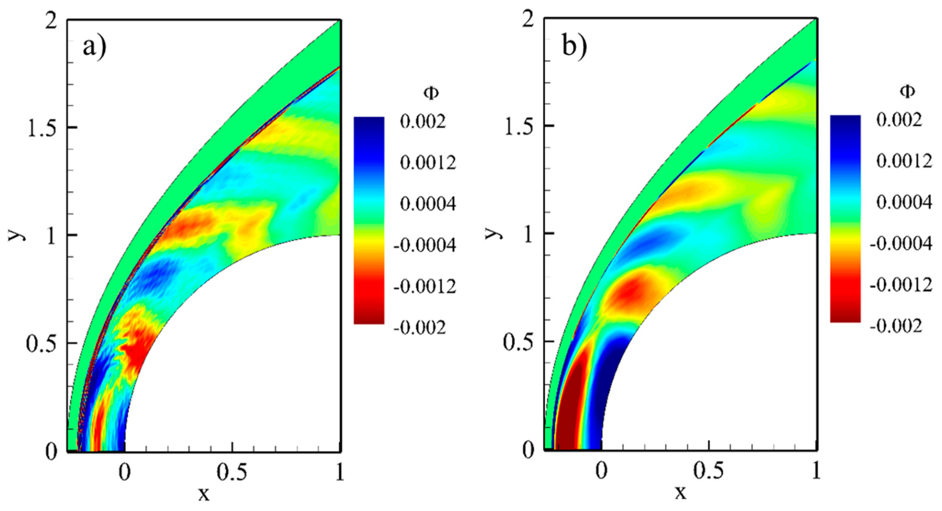
4.6. Coherent Structure of the Experimental Modes

By observing the spatial structure of the modes oscillating around the experimental frequency as shown in Figure 24, it can be seen that for a regularly oscillating flow field, the fluctuation occurs primarily at two locations: one is near the reaction zone along the stagnation streamline; and the other fluctuation is around the projectile surface where the compression waves emanating from the reaction zone are reflected. With the instability mode, the location of the compression waves being reflected stays near the stagnation point of the projectile surface. In our earlier study [46], we analyzed the same instability mechanism using a one-dimensional DMD approach and chemical explosive mode analysis (CEMA), and it was found that the sensitivity of the high-temperature reactions triggers the fluctuations. The fluctuation slows, develops instability, and decouples the regularly oscillating mechanism and, finally, leads to an unphysical flow field similar to that of the large disturbance regimes (LDR) as observed in similar experiments at other flying conditions. With the Dryer mechanism, initially, a mild disturbance is created at the interaction of the reflected and incoming pressure waves in the reaction zone. This additionally triggers combustion in the reaction zone and creates a more substantial pressure wave which moves towards the projectile surface and is reflected to interact with the incoming wave. This again triggers the combustion further, and this process repeats, eventually converting the regular mode of oscillation into instability.

5. Conclusions

Shock-induced combustion is an exothermic flow phenomenon where the chemical kinetics control the exothermicity. The exothermic flow is inherently unstable, where the instability of shock-induced combustion arose. The instability of shock-induced combustion can be classified into a high-frequency regular oscillation regime and a low-frequency large-disturbance regime. Experimental results for the present case of Mach number 4.48 by Lehr [7] is well known as high-frequency regular oscillation; however, some of the present case results show the transition of instability from the high-frequency regular oscillation regime to the low-frequency large-disturbance regime, which is not observed in the experiment. Clearly, the transition appears as the numerical dissipation is reduced by increasing the grid resolution.
In this study, the sensitivity of the reaction mechanisms for the SIC was studied. Various kinetic models were used to simulate the SIC flow field and it was found that some reaction mechanisms were grid-sensitive with higher-order schemes for high-speed combustion applications. Jachimowski mechanisms as well as Dryer mechanisms were highly sensitive to the grid resolution. The UCSD reaction mechanism was grid-insensitive and did not develop any spurious oscillation with third-order numerical schemes while other reaction mechanisms developed instability because of the spurious oscillations. Since the transition was not observed in the experiment, the authors concluded that the UCSD and USC mechanisms which did not demonstrate the transition in the refined grid system are more accurate or reliable than other mechanisms. The UCSD and USC mechanisms also displayed better agreement for ignition delay and flame speed.
Using the decomposition analysis, the structure of the modes was analyzed to understand the phenomena that cause this instability in the numerical simulation of unsteady shock-induced combustion. The spatial structure of the decomposed modes extracts the location where the impact is dominant at that frequency. From this analysis, it is found that the compression waves reflecting from the projectile surface are coupled with the reaction zone in a regularly oscillating flow field. With the instability mode, this mechanism is decoupled and occurs at a different frequency which leads to the unphysical oscillation of the leading shock wave.

Author Contributions

Conceptualization, P.K.P. and J.-Y.C.; methodology, P.K.P. and J.-Y.C.; software, P.K.P. and J.-Y.C.; validation, P.K.P. and J.-Y.C.; formal analysis, P.K.P.; investigation, P.K.P., M.-S.J. and J.-Y.C.; resources, J.-E.K. and J.-Y.C.; data curation, P.K.P., M.-S.J.; writing—original draft preparation, P.K.P.; writing—review and editing, M.-S.J. and J.-E.K.; visualization, P.K.P., M.-S.J.; supervision, J.-Y.C.; project administration, J.-Y.C. and M.-S.J.; funding acquisition, J.-Y.C. All authors have read and agreed to the published version of the manuscript.

Funding

This work was supported by the National Research Foundation (NRF) of Korea grant (NRF-2019R1A2C1004505 and NRF-2022M1A3C2076724) funded by the Ministry of Science and ICT (MSIT) of the Republic of Korea Government. Publication of this paper and fellowship to J.-E. Kim and M.-S. Jo were supported by the BK21 FOUR (Fostering Outstanding Universities for Research) fellowship funded by the Ministry of Education (MOE, Korea) and National Research Foundation of Korea (NRF).

Data Availability Statement

The data presented in this study are openly available in [23,24,25,26,27,28,29,30,31,32,33,34,35,36].

Conflicts of Interest

The authors declare that they have no known competing financial interests or personal relationships that could have appeared to influence the work reported in this paper.

References

  1. Ruegg, F.W.; Dorsey, W.W. A missile technique for the study of detonation waves. J. Res. Natl. Bur. Stand. C 1962, 66, 51–58. [Google Scholar] [CrossRef]
  2. Behrens, H.; Struth, W.; Wecken, F. Studies of hypervelocity firings into mixtures of hydrogen with air or with oxygen. Symp. Combust. 1965, 10, 245–252. [Google Scholar] [CrossRef]
  3. Chernyi, G. Supersonic flow past bodies with formation of detonation and combustion fronts. Acta Astronaut. 1968, 13, 467–480. [Google Scholar]
  4. McVey, J.B. Mechanism of Instabilities of Exothermic Hypersonic Blunt-Body Flows. Combust. Sci. Technol. 1971, 3, 63–76. [Google Scholar] [CrossRef]
  5. Alpert, R.L.; Toong, T.Y. Periodicity in exothermic hypersonic flows about blunt projectiles. Acta Astronaut. 1972, 17, 539–560. [Google Scholar]
  6. Toong, T.Y. Instabilities in reacting flows. Acta Astronaut. 1974, 1, 317–344. [Google Scholar] [CrossRef]
  7. Lehr, H.F. Experiments on Shock-Induced Combustion. Acta Astronaut. 1972, 17, 589–597. [Google Scholar]
  8. Kailasanath, K. Review of propulsion applications of detonation waves. AIAA J. 2000, 38, 1698–1708. [Google Scholar] [CrossRef]
  9. Nejaamtheen, M.N.; Kim, J.-M.; Choi, J.-Y. Review on the research progresses in rotating detonation engine. In Detonation Control for Propulsion: Pulse Detonation and Rotating Detonation Engines; Springer: Berlin/Heidelberg, Germany, 2018; pp. 109–159. [Google Scholar]
  10. Anand, V.; Gutmark, E. Rotating detonation combustors and their similarities to rocket instabilities. Prog. Energy Combust. Sci. 2019, 73, 182–234. [Google Scholar] [CrossRef] [Green Version]
  11. Yungster, S.; Eberhardt, S.; Bruckner, A.P. Numerical simulation of hypervelocity projectiles in detonable gases. AIAA J. 1991, 29, 187–199. [Google Scholar] [CrossRef]
  12. Yungster, S.; Radhakrishnan, K. A fully implicit time accurate method for hypersonic combustion: Application to shock-induced combustion instability. Shock Waves 1996, 5, 293–303. [Google Scholar] [CrossRef]
  13. Wilson, G.J.; Sussman, M.A. Computation of unsteady shock-induced combustion using logarithmic species conservation equations. AIAA J. 1993, 31, 294–301. [Google Scholar] [CrossRef]
  14. Matsuo, A.; Fujiwara, T. Numerical investigation of oscillatory instability in shock-induced combustion around a blunt body. AIAA J. 1993, 31, 1835–1841. [Google Scholar] [CrossRef]
  15. Matsuo, A.; Fujii, K. Computational study of large-disturbance oscillations in unsteady supersonic combustion around projectiles. AIAA J. 1995, 33, 1828–1835. [Google Scholar] [CrossRef]
  16. Matsuo, A.; Fujii, K.; Fujiwara, T. Flow features of shock-induced combustion around projectile traveling at hypervelocities. AIAA J. 1995, 33, 1056–1063. [Google Scholar] [CrossRef]
  17. Choi, J.-Y.; Jeung, I.-S.; Yoon, Y. Computational fluid dynamics algorithms for unsteady shock-induced combustion, part 1: Validation. AIAA J. 2000, 38, 1179–1187. [Google Scholar] [CrossRef]
  18. Choi, J.-Y.; Jeung, I.-S.; Yoon, Y. Computational fluid dynamics algorithms for unsteady shock-induced combustion, part 2: Comparison. AIAA J. 2000, 38, 1188–1195. [Google Scholar] [CrossRef]
  19. Jachimowski, C.J. Analytical Study of the Hydrogen-Air Reaction Mechanism with Application to Scramjet Combustion; NASA Technical Paper No. 2791; NASA: Washington, DC, USA, 1988. [Google Scholar]
  20. Jachimowski, C.J. An Analysis of Combustion Studies in Shock Expansion Tunnels and Reflected Shock Tunnels; NASA Technical Paper No. 3224; NASA: Washington, DC, USA, 1992. [Google Scholar]
  21. Clutter, J.K.; Mikolaitis, D.W.; Shyy, W. Reaction mechanism requirements in shock-induced combustion simulations. Proc. Combust. Inst. 2000, 28, 663–669. [Google Scholar] [CrossRef]
  22. Pavalavanni, P.K.; Kim, K.-S.; Oh, S.; Choi, J.-Y. Numerical comparison of hydrogen-air reaction mechanisms for unsteady shock-induced combustion applications. J. Mech. Sci. Technol. 2015, 29, 893–898. [Google Scholar]
  23. Olm, C.; Zsély, I.G.; Pálvölgyi, R.; Varga, T.; Nagy, T.; Curran, H.J.; Turányi, T. Comparison of the performance of several recent hydrogen combustion mechanisms. Combust. Flame 2014, 161, 2219–2234. [Google Scholar] [CrossRef] [Green Version]
  24. Ströhle, J.; Myhrvold, T. An evaluation of detailed reaction mechanisms for hydrogen combustion under gas turbine conditions. Int. J. Hydrog. Energy 2007, 32, 125–135. [Google Scholar] [CrossRef]
  25. GRI-Mech 3.0. Available online: http://combustion.berkeley.edu/gri-mech/version30/text30.html (accessed on 27 December 2022).
  26. Maas, U.; Warnatz, J. Ignition processes in hydrogen-oxygen mixtures. Combust. Flame 1988, 74, 53–69. [Google Scholar] [CrossRef]
  27. Conaire, M.Ó.; Curran, H.J.; Simmie, J.M.; Pitz, W.J.; Westbrook, C.K. A comprehensive modeling study of hydrogen oxidation. Int. J. Chem. Kinet. 2004, 37, 603–622. [Google Scholar] [CrossRef]
  28. Li, J.; Zhao, Z.; Kazakov, A.; Dryer, F.L. An updated comprehensive kinetic model of hydrogen combustion. Int. J. Chem. Kinet. 2004, 36, 566–575. [Google Scholar] [CrossRef]
  29. Petersen, E.L.; Hanson, R.K. Reduced Kinetics Mechanisms for Ram Accelerator Combustion. J. Propuls. Power 1999, 15, 591–600. [Google Scholar] [CrossRef]
  30. Burke, M.P.; Chaos, M.; Ju, Y.; Dryer, F.L.; Klippenstein, S.J. Comprehensive H2/O2 kinetic model for high-pressure combustion. Int. J. Chem. Kinet. 2012, 44, 444–474. [Google Scholar] [CrossRef]
  31. USC Mech Version II. High-Temperature Combustion Reaction Model of H2/CO/C1-C4 Compounds. Available online: http://ignis.usc.edu/USC_Mech_II.htm (accessed on 27 December 2022).
  32. Williams, F.A.; Seshadri, K.; Cattolica, R. Chemical-Kinetic Mechanisms for Combustion Applications. Available online: http://combustion.ucsd.edu (accessed on 27 December 2022).
  33. MECHMOD v. 1.4: Program for the Transformation of Kinetic Mechanisms. Available online: http://www.chem.leeds.ac.uk/Combustion/Combustion.html (accessed on 27 December 2022).
  34. RESPECTH. Available online: http://respecth.chem.elte.hu/respecth/index.php (accessed on 27 December 2022).
  35. Kao, S.; Shepherd, J. Numerical solution methods for control volume explosions and ZND detonation structure. GALCIT Rep. 2006, 7, 1–46. [Google Scholar]
  36. Kéromnès, A.; Metcalfe, W.K.; Heufer, K.A.; Donohoe, N.; Das, A.K.; Sung, C.-J.; Herzler, J.; Naumann, C.; Griebel, P.; Mathieu, O.; et al. An experimental and detailed chemical kinetic modeling study of hydrogen and syngas mixture oxidation at elevated pressures. Combust. Flame 2013, 160, 995–1011. [Google Scholar] [CrossRef] [Green Version]
  37. JovanoviĆ, M.R.; Bamieh, B. Componentwise energy amplification in channel flows. J. Fluid Mech. 2005, 534, 145–183. [Google Scholar] [CrossRef] [Green Version]
  38. Schmid, P.J. Nonmodal Stability Theory. Annu. Rev. Fluid Mech. 2006, 39, 129–162. [Google Scholar] [CrossRef] [Green Version]
  39. Bagheri, S. Koopman-mode decomposition of the cylinder wake. J. Fluid Mech. 2013, 726, 596–623. [Google Scholar] [CrossRef]
  40. Jeong, S.-M.; Choi, J.-Y. Combined Diagnostic Analysis of Dynamic Combustion Characteristics in a Scramjet Engine. Energies 2020, 13, 4029. [Google Scholar] [CrossRef]
  41. Quinlan, J.M. Investigation of Driving Mechanisms of Combustion Instabilities in Liquid Rocket Engines Via the Dynamic Mode Decomposition. Ph.D. Thesis, Georgia Institute of Technology, Atlanta, GA, USA, 10 August 2015. [Google Scholar]
  42. Hwang, W.-S.; Sung, B.-K.; Han, W.; Huh, K.Y.; Lee, B.J.; Han, H.S.; Sohn, C.H.; Choi, J.-Y. Real-Gas-Flamelet-Model-Based Numerical Simulation and Combustion Instability Analysis of a GH2/LOX Rocket Combustor with Multiple Injectors. Energies 2021, 14, 419. [Google Scholar] [CrossRef]
  43. Richecoeur, F.; Hakim, L.; Renaud, A.; Zimmer, L. DMD algorithms for experimental data processing in combustion. In Proceedings of the CTR Summer Program, Los Angeles, CA, USA, 14 December 2012. [Google Scholar]
  44. Torregrosa, A.J.; Broatch, A.; García-Tíscar, J.; Gomez-Soriano, J. Modal decomposition of the unsteady flow field in compression-ignited combustion chambers. Combust. Flame 2018, 188, 469–482. [Google Scholar] [CrossRef]
  45. Schmid, P.J. Dynamic mode decomposition of numerical and experimental data. J. Fluid Mech. 2010, 656, 5–28. [Google Scholar] [CrossRef] [Green Version]
  46. Pavalavanni, P.K.; Sohn, C.H.; Lee, B.J.; Choi, J.-Y. Revisiting unsteady shock-induced combustion with modern analysis techniques. Proc. Combust. Inst. 2019, 37, 3637–3644. [Google Scholar] [CrossRef]
Figure 1. Experimental shadowgraph of periodical oscillation observed taken at 12° angle from perpendicular direction for M = 4.48 in Lehr’s experiment [7].
Aerospace 10 00292 g001
Figure 2. Computational domain for the analysis of shock-induced combustion with Nx × Ny grid system.
Aerospace 10 00292 g002
Figure 3. Ignition delays calculated at 1 bar (symbol represents the experimental results from ReSpecTh repository).
Aerospace 10 00292 g003
Figure 4. Ignition delays calculated at 10 bar (symbol represents the experimental results from ReSpecTh repository).
Aerospace 10 00292 g004
Figure 5. Laminar burning velocity calculated for initial temperature 298 K and 1 bar (symbols represent the experimental results from ReSpecTh repository).
Aerospace 10 00292 g005
Figure 6. Laminar burning velocity calculated for initial temperature 298 K and 10 bar.
Aerospace 10 00292 g006
Figure 7. Temperature profile for various reaction mechanisms calculated from the CV explosion model.
Aerospace 10 00292 g007
Figure 8. Pressure profile for various reaction mechanisms calculated from the CV explosion model.
Aerospace 10 00292 g008
Figure 9. Overview of the numerical results for regularly oscillating shock-induced combustion case flying at Mach 4.48. Color scale of x-t diagram is the same as the contour plot.
Aerospace 10 00292 g009
Figure 10. Pressure probed along the stagnation point for various grid resolutions (red—150 × 200; green—200 × 300; blue—300 × 450; and black—400 × 600).
Aerospace 10 00292 g010
Figure 11. Mach contour of the shock-induced combustion at Mach number 4.48 with various reaction mechanisms (300 × 450 grid system) compared with experimental shadowgraph image [7] (min 0, max 4.48, increment 0.04, colored with Mach number).
Aerospace 10 00292 g011
Figure 12. The x-t graph of SIC probed along the stagnation streamline for various reaction mechanism at 150 × 200 grid resolution. Color scale is the same as Figure 9.
Aerospace 10 00292 g012
Figure 13. The x-t graph of SIC probed along the stagnation streamline for various reaction mechanism at 400 × 600 grid resolution. Color scale is the same as Figure 9.
Aerospace 10 00292 g013
Figure 14. Streamline extraction of the temperature contour for the Jachimowski-92 mechanism at various grid levels. Color scale is the same as Figure 9.
Aerospace 10 00292 g014
Figure 15. Streamline extraction of the temperature contour for the Dryer mechanism at various grid levels. Color scale is the same as Figure 9.
Aerospace 10 00292 g015
Figure 16. Attenuation of the instability phenomena observed with the Jachimowski-88 mechanism at 400 × 600 grid system. Color scale is the same as Figure 9.
Aerospace 10 00292 g016
Figure 17. Temporal characteristics of decomposed modes using DMD with UCSD reaction mechanism for 200 × 300 grid resolution (red dot—growth factor; blue line—normalized coherence).
Aerospace 10 00292 g017
Figure 18. Energy distribution among the decomposed modes using POD with UCSD reaction mechanism for 200 × 300 grid resolution.
Aerospace 10 00292 g018
Figure 19. Dominant spatial coherent structures extracted from DMD and POD analysis.
Aerospace 10 00292 g019
Figure 20. Temporal characteristics and spatial coherent structure of the flow field with DMD analysis for with UCSD reaction mechanism for 400 × 600 grid resolution (red dot—growth factor; blue line—normalized coherence). DMD color scale is the same as Figure 19.
Aerospace 10 00292 g020
Figure 21. Spatial coherent structure of the flow field with POD analysis for with UCSD reaction mechanism for 400 × 600 grid resolution (E represents normalized eigen value.). POD color scale is the same as Figure 19.
Aerospace 10 00292 g021
Figure 22. Temporal characteristics and spatial coherent structure of the flow field with DMD analysis for with the Dryer reaction mechanism for 400 × 600 grid resolution (red dot—growth factor; blue line—normalized coherence). DMD color scale is the same as Figure 19.
Aerospace 10 00292 g022
Figure 23. Spatial coherent structure of the flow field with POD analysis for with the Dryer reaction mechanism for 400 × 600 grid resolution (E represents normalized eigen value). POD color scale is the same as Figure 19.
Aerospace 10 00292 g023
Figure 24. Experimental DMD modes: (a) Dryer mechanism at 408.3 kHz; and (b) UCSD mechanism at 419.2 kHz.
Aerospace 10 00292 g024
Table 1. Ignition delays calculated from the constant volume explosion model.
Reaction MechanismIgnition Delay (μs)
Conaire2.537
Kéromnès2.983
Jachimowski 882.194
Jachimowski 922.466
GRI Mech 3.07.444
Dryer3.005
UCSD2.811
USC2.676
Table 2. Flow field oscillation calculated for various reaction mechanisms.
Reaction Mechanism150 × 200200 × 300300 × 450400 × 600
Jachimowski (1988)430.2444.6428.175.0/330.0
Jachimowski (1992)408.4/41.0416.776.2/51372.2/360.0
Dryer397.280.0/413.879.0/35174.9/335.0
GRI Mech 3.0226.0230.35220.5208.5
UCSD416.5431.3415.4409.4
USC416.7427.0411.1398.0
Disclaimer/Publisher’s Note: The statements, opinions and data contained in all publications are solely those of the individual author(s) and contributor(s) and not of MDPI and/or the editor(s). MDPI and/or the editor(s) disclaim responsibility for any injury to people or property resulting from any ideas, methods, instructions or products referred to in the content.

