1. Introduction
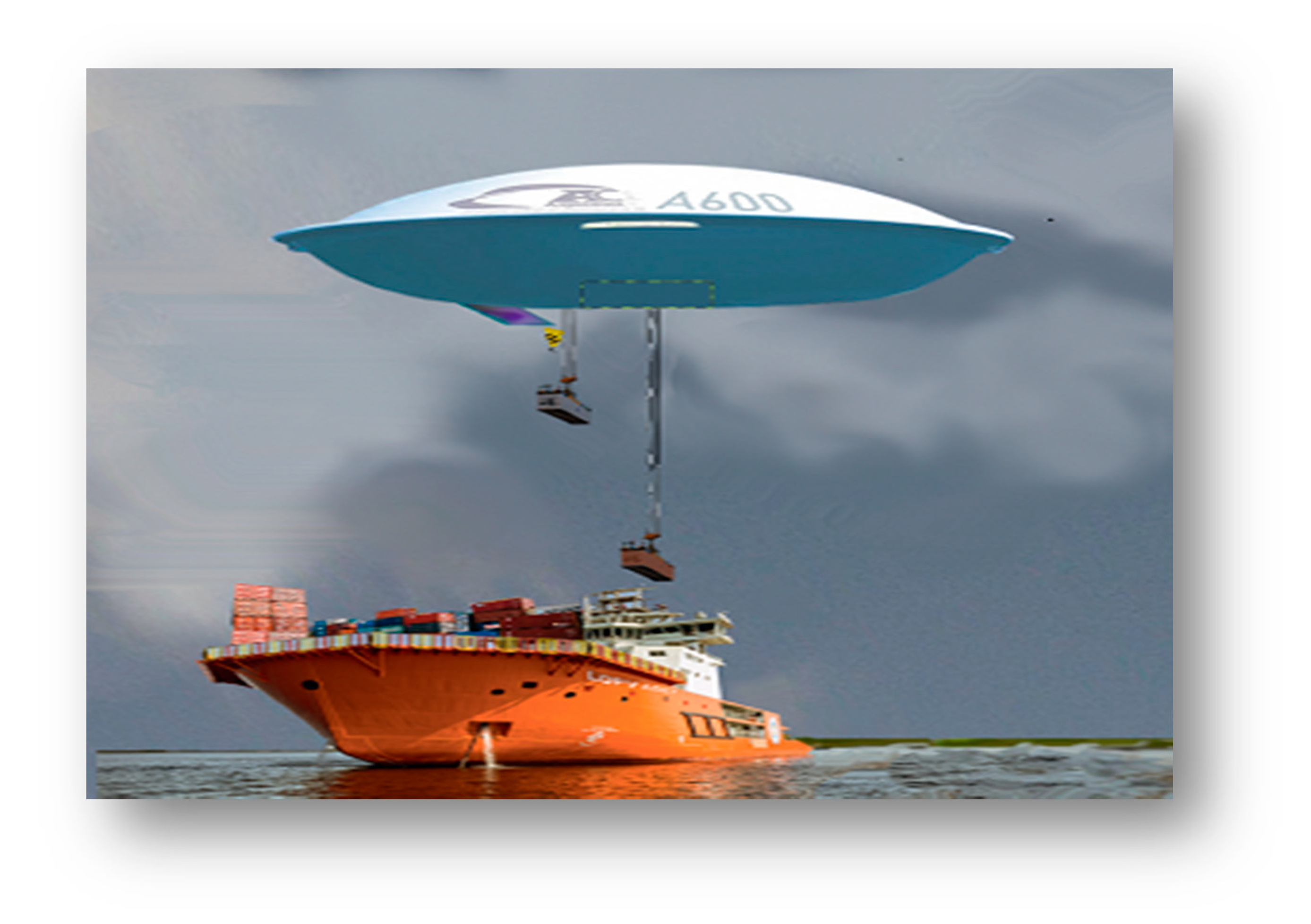
Large capacity airships (LCAs) bring new perspectives for airships that hibernated for more than half a century after the Hindenburg drama. In fact, for more than two decades, researchers have studied the formidable potential of airships in terms of freight transport. These airships will be able to transport blades of wind turbines or logs from or to areas very difficult to access, load or unload container ships on the high seas in the absence of adequate ports (as seen in
Figure 1), and install field hospitals in disaster areas. Other examples of the use of airships in land and maritime multimodal logistics can be found in [
1,
2]. These various examples prove, if necessary, the enormous potential available to these flying machines. However, we should mention that in order to be able to lift 1 kg of load, 1 m
3 of Helium must be provided within the hull of the airship. The airships targeted for the aforementioned examples will therefore have enormous volumes, and all the obstacles inherent in these large volumes have not yet been overcome. Among these obstacles, we note on the one hand, the high sensitivity of airships to gusts of wind. Various studies have looked into the stabilization of airships, particularly in hovering flight or for tracking trajectories (see, for example, [
3,
4,
5,
6,
7]). On the other hand, the non-standard dimensions of these devices make the development of landing or handling areas very problematic or costly. This has left the designers of these machines to consider handling operations at altitude. It is in this context that our study takes place. We propose for this task a smart crane capable not only of loading and unloading but also of stabilizing the load during a gust of wind and of arranging the hold of the airship. This crane will be based on a cable-driven parallel manipulator (CDPM).
Today, CDPMs are set to have a big impact on many aspects of modern life, from industrial manufacturing to healthcare, transportation, and the exploration of space and the seabed. Cable-driven parallel manipulators are a special class of parallel manipulators in which the effector is directly actuated by cables. By considering the number of cables and the degrees of freedom of the effector, the CDPM can be overconstrained, in particular as in [
8,
9], or underconstrained.
These manipulators offer a variety of potential advantages over traditional parallel robots. Because of their unique configurations, CDPMs are characterized by light structures and a large working space due to the location of the actuators at the fixed base of the structure, thus reducing the mass and inertia of the mobile platform. They can be produced on a very large scale at acceptable cost, which makes them very suitable for high velocities and high performance [
10,
11]. Another major advantage is that the CDPMs are reconfigurable, which allows them to be used for different tasks by moving the attachment points of cables as in [
12].
In the literature, different approaches have been proposed to find the tension distribution of cables. The set of optimal tension chosen is usually performed using an optimization method, for example, linear programming [
13], quadratic programming [
14], and convex optimization for the minimization of L1 norm [
15] and p norm [
16]. However, neither of these methods can provide a continuous solution and cover the entire workspace as in [
17]. Another disadvantage of cable parallel robots is the possibility of cables colliding with each other, but this is limited only to space redundant systems as in [
12].
Given the advantages and unique characteristics of CDPMs, their use has spread to several types of applications. The idea of cable robots appeared from the studies of Albus et al. [
18], Landsberger [
19], and Higuchi [
20]. Inspired by Stewart platform, the NIST-Robot Crane was developed by Albus and his team [
18] to overcome the drawbacks of the motions underlying conventional cranes. Because of their large workspace and high velocities, the CDPMs have been used in sports recording, as in the case of Skycam [
21]. Another application for this type of manipulator is medical rehabilitation as can be seen in [
22,
23,
24].
We were therefore inspired by the CDPM principle to propose our smart crane on board the airship, the design of which we will present in the next section.
A model of a multibody system formed by the airship, the crane, and the suspended load will be presented, and the stabilization of the system subjected to a gust of wind will be proposed.
2. Problem Statement and Description of the Smart Crane
As part of the development of tools essential to the development of large capacity airships, we set out to design an embedded smart crane (the CHAYA-SC) that is as light as possible, can both handle the containers and stabilize the load during the handling, and finally ensure the precise arrangement of the containers within the hold.
The large airships that we are targeting have a large volume, greater than 100,000 m3, and it would be difficult to provide them with landing and loading infrastructure. So that these means of transport could be used everywhere, it is essential to provide a means of handling at altitude. This will allow them to be used universally but must be accompanied by various measures, in particular robust control of the airship and a crane adapted to this configuration. It is in this context that we present our smart crane.
Presentation of the Smart Crane
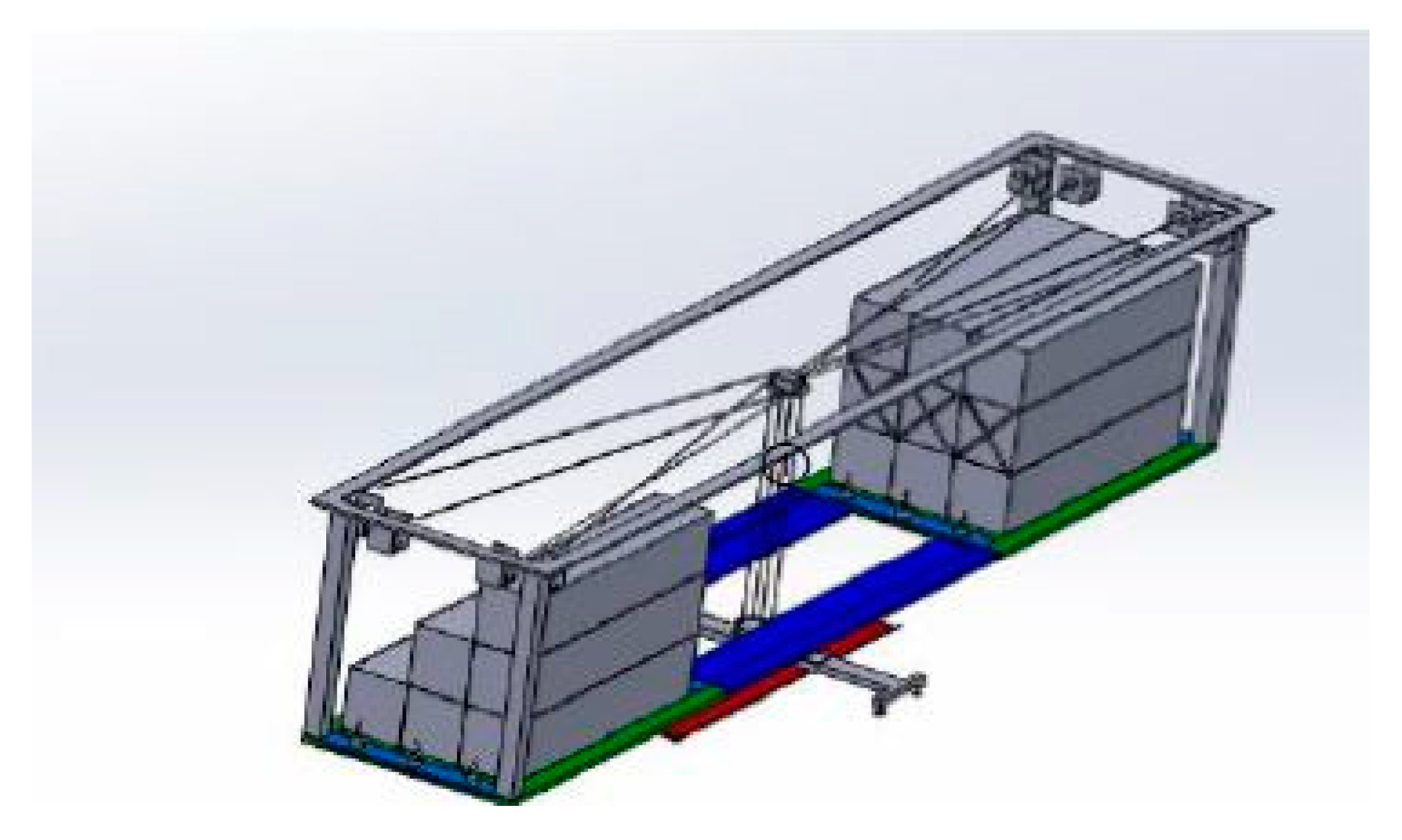
The smart crane called CHAYA-SC is presented in
Figure 2. It consists of a cuboid trunk (that we could see in details in
Figure 3) supported by eight cables suspended from the four upper corners of the airship hold. These eight cables are arranged to kinematically constrain the trunk.
Eight winches have the role of controlling these eight cables. These are controlled and coordinated by a computer. The motion of the platform is controlled by an operator through a six-axis joystick with six DOFs. The operator can handle and manipulate the trunk and any load attached to it over a large volume of work inside the hold.
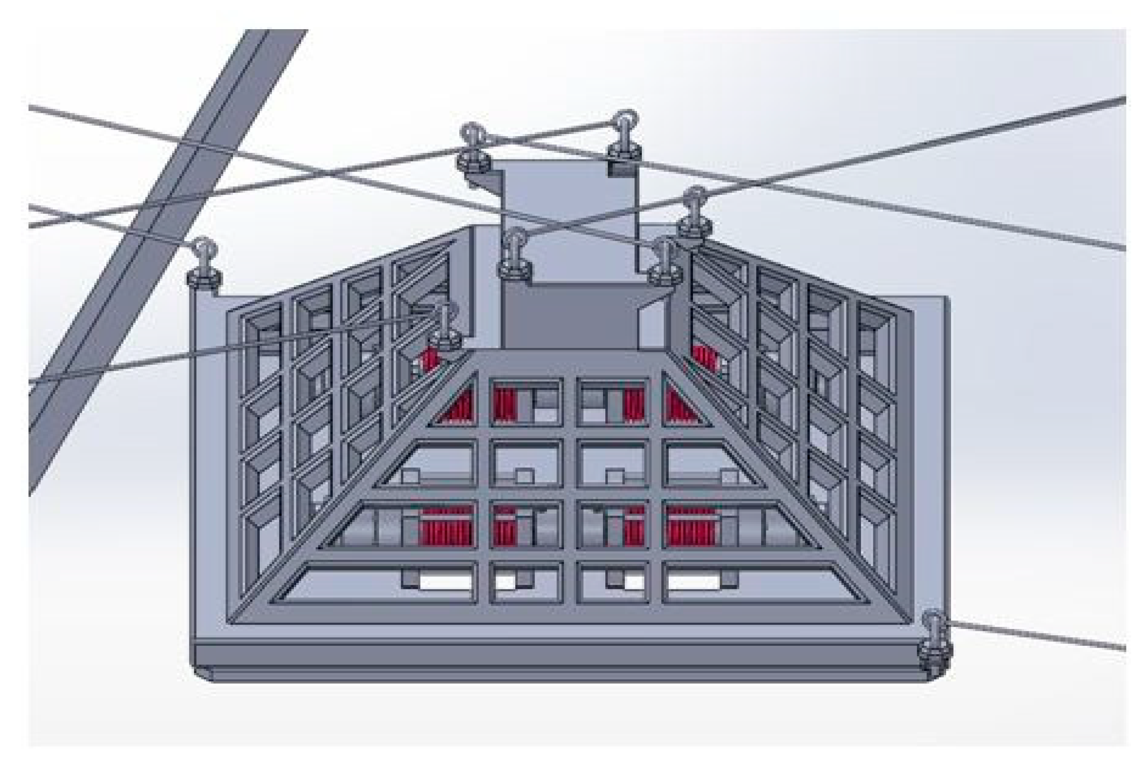
The trunk consists of a rigid structure overhung by four electrical engines. These engines pull a flexible cable connected to a container hook. The multiplication of electrical engines obeys safety constraints.
This crane has the following missions:
- 1.
A classic container loading and unloading mission enabled by the winches integrated into the cuboid.
- 2.
Stabilize the suspended containers during a sudden motion of the airship under the effect of a gust of wind by creating accelerations according to six possible degrees of freedom of the cuboid, depending on the nature of the oscillation of the load.
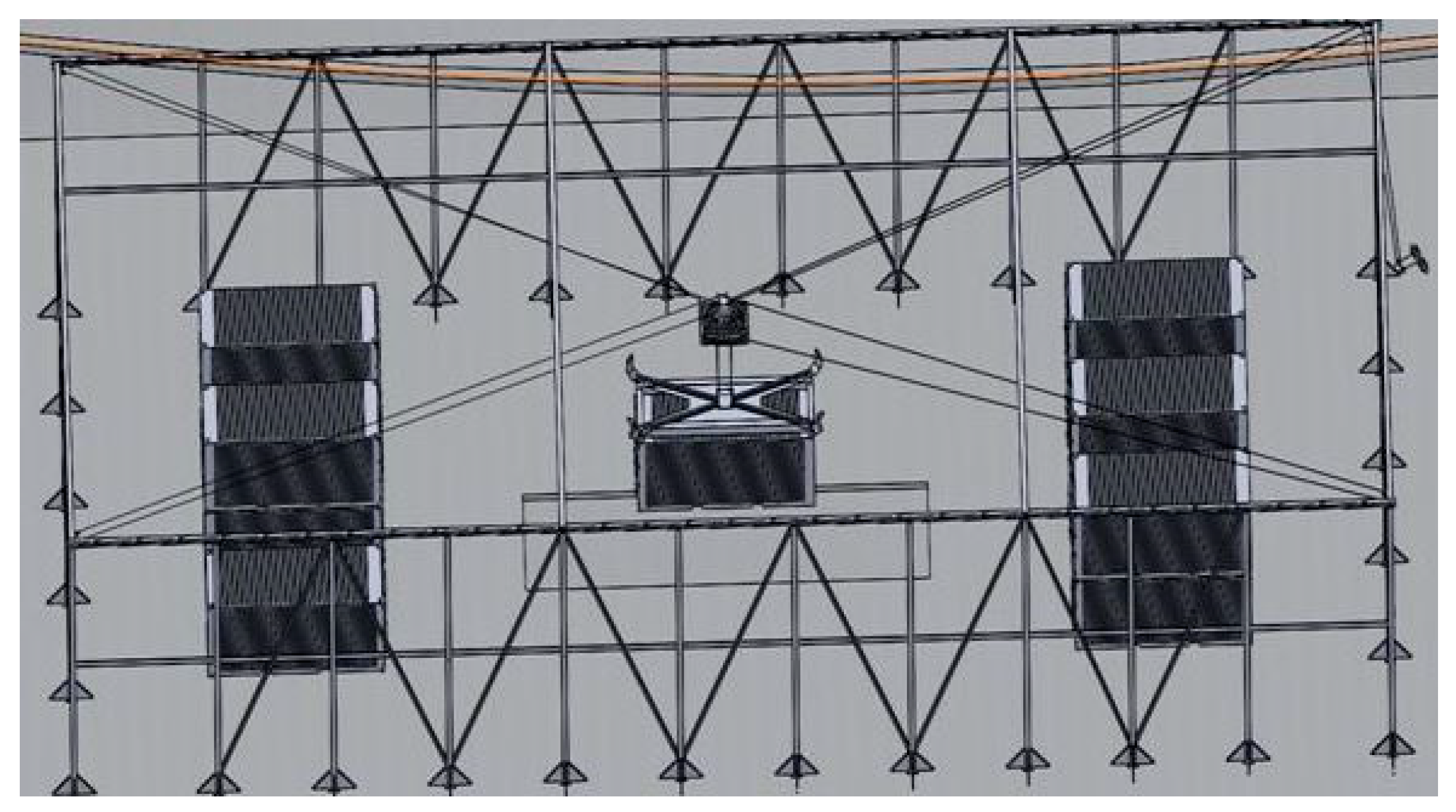
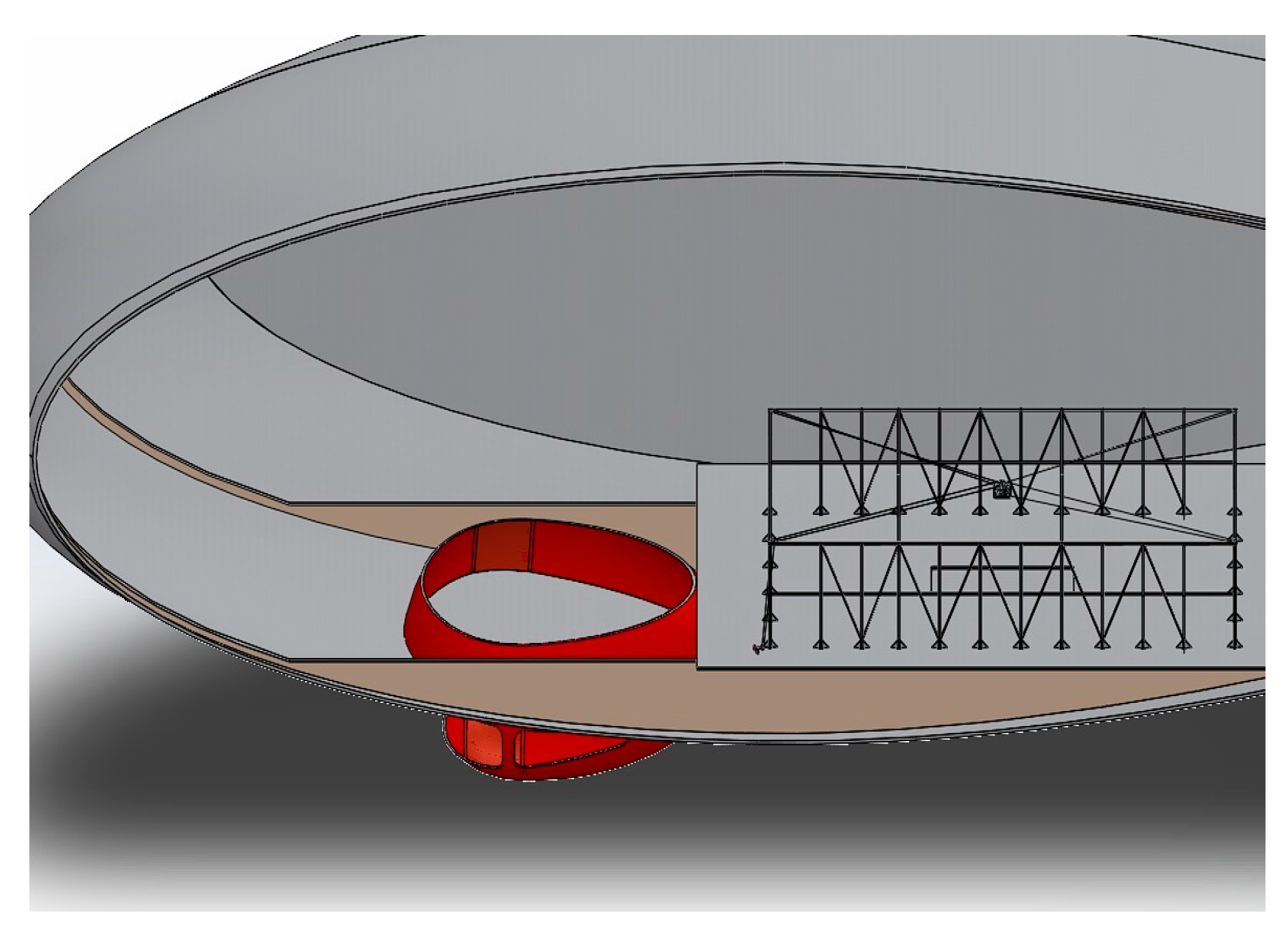
- 3.
Drop off, collect, and store the containers in the airship hold (as shown in
Figure 4).
3. Dynamic Modelling
3.1. Modeling of the Cable-Driven Parallel Manipulator
3.1.1. Classical Case: Industrial CDPM
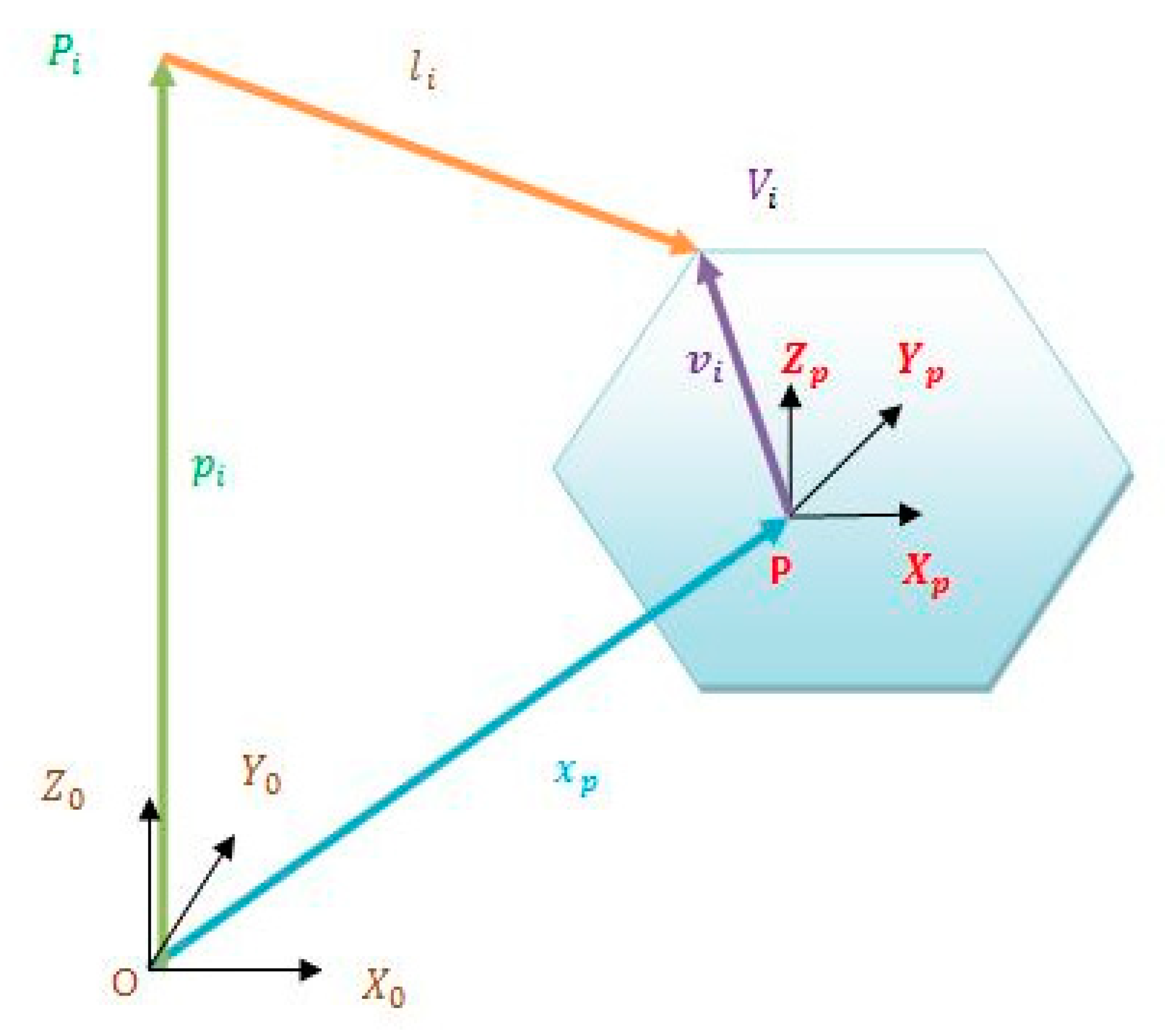
Let us consider a CDPM with m cables having the geometry illustrated in
Figure 5.
The cables are attached to the fixed base at the exit points noted whose coordinates are defined in the earth fixed frame by the vectors . The cable attachment points on the platform noted are expressed in the mobile frame attached to the suspended platform by , and is the length of the cable connecting these two points.
Unlike series-type robots, the inverse geometric and inverse kinematic models of parallel robots are easy to establish. These results are used to find a relation between the operational space with n dimensions of the spatial coordinates of the platform and the space with m dimensions of the articular coordinates.
We denote by the column matrix of the articular coordinates of the CDPM and by the operational coordinates of the platform.
The inverse kinematics problem seeks to determine the lengths of the cables taking into account the position and orientation of the suspended platform. Inverse kinematics for parallel structures is easier to calculate than direct kinematics. The Jacobian matrix J of a cable-driven parallel robot is defined as a relationship between the velocity vector of the platform
and the linear velocity of the cables
:
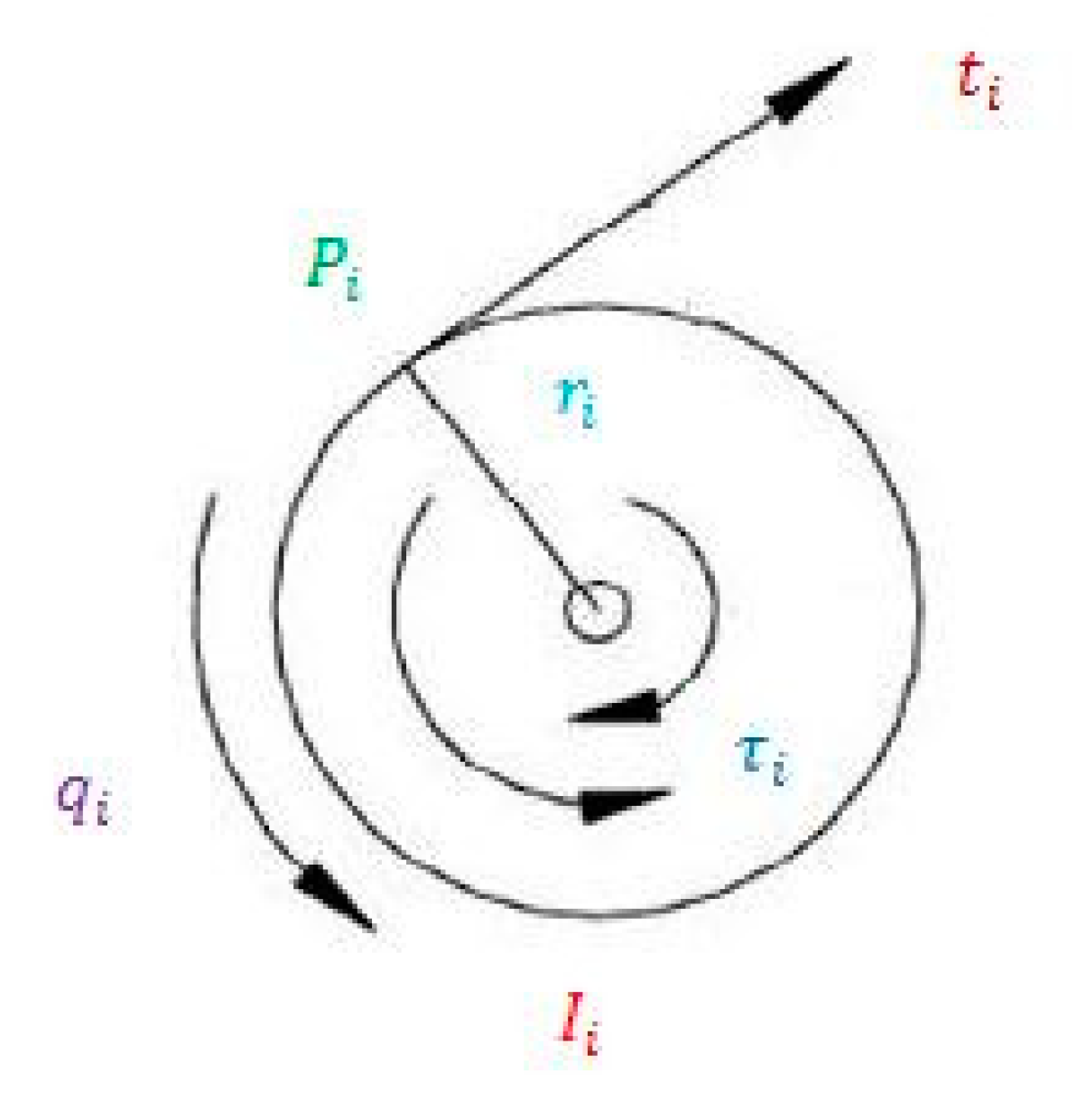
The dynamic equations which describe the motion of the CDPM are obtained using the Lagrange equations that we will recall later in this paper. The general dynamic model can be divided into two expressions corresponding to the dynamics of the platform and the dynamics of the winches. The cables are considered in deformable and of negligible mass. The cables are controlled by motorized winches. These winches are equipped with a drum around which a cable is wound. Each winch (
Figure 6) consists of asynchronous servomotor coupled to a planetary gearbox which is connected to a drum. In fact, the motor torques
τi drives the cylindrical drum in rotation at an angle
qi about its axis of symmetry. This generates a tensile force
ti at the exit point of the cable
Pi.
The dynamic model of the actuators is given by the following equation:
is the input vector of the torques exerted by the motors which control synchronously the cable lengths as a function of the tension in order to provide the required movement of the platform in the Cartesian space by acting on the winches, and I is the diagonal inertia matrix of the moments of the drums, such as .
By applying the Lagrange equations, the dynamic equation of the lower base will be given, as in [
25], by:
Fg represents the external forces, such as the weight of the platform and its loading or the force exerted by a gust of wind,
,
M is the mass matrix of the platform,
C is the matrix of centrifugal and Coriolis forces. The latter two are defined in detail in
Appendix C.
3.1.2. Case of the CDPM on Board an Airship
The CDPM which represents the upper part of our smart crane and which we present in this work is inspired by those used in industry from a technological and configuration point of view. We were inspired more precisely by the robot CoGiRo developed by Tecnalia presented in [
26], which corresponds to our handling needs. In their study, Lamaury et al. defined the appropriate number of cables for the optimal control of the movement of the cuboid according to the six degrees of freedom. Their study concluded that this would require the use of eight cables. We followed this recommendation and used eight cables to manipulate the cuboid of our smart crane.
The main difference between these two CDPMs (apart from the dimensional aspect) is that ours is embarked on a mobile system (the airship) and is therefore subject to the turbulence and acceleration of the latter. The so-called “fixed” base actually follows the motion of the airship.
The mobile platform is embodied by the cuboid in our smart crane. Its motion depends not only on the motion of the eight cables that support it but also on the motion of the airship.
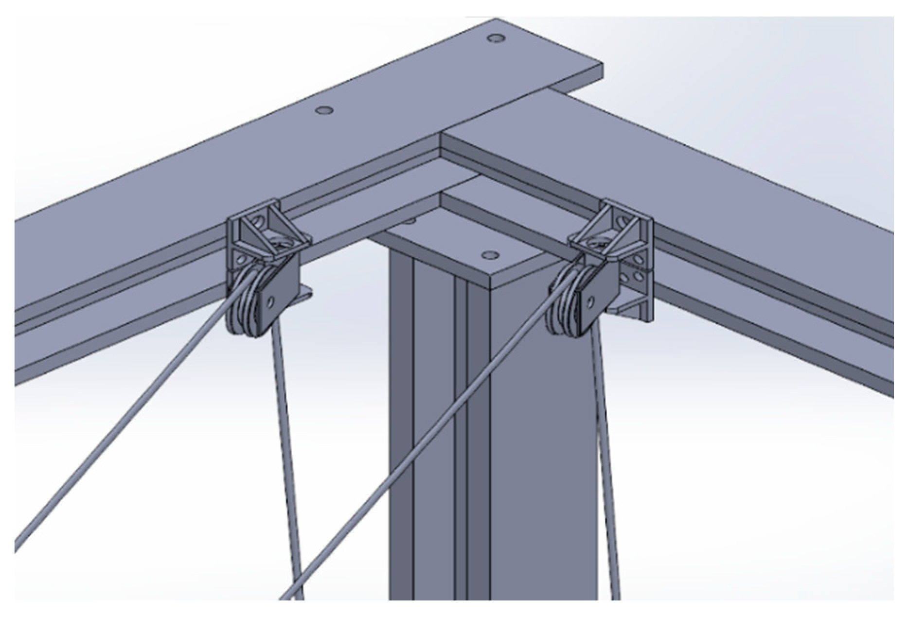
The CDPM is suspended by eight cables for six DOFs. The cables are connected on the other side to the hold of the airship at the top of the pillars (as seen in
Figure 7). Each point of attachment of the cables is therefore directly deduced from the motion of the center of gravity G of the airship.
The pulleys guiding the cables (as shown in
Figure 8) are connected to controlled motors which represent the actuators of the CDPM.
The set of forces exerted on the platform (cuboid) is given by:
Compared to the equations developed previously and neglecting the term
, we will have to use the kinetic energy of the airship to obtain the equation of motion of the CDPM:
More details concerning the obtaining of this equation will be developed in the particular case of the plane motion of the multibody system.
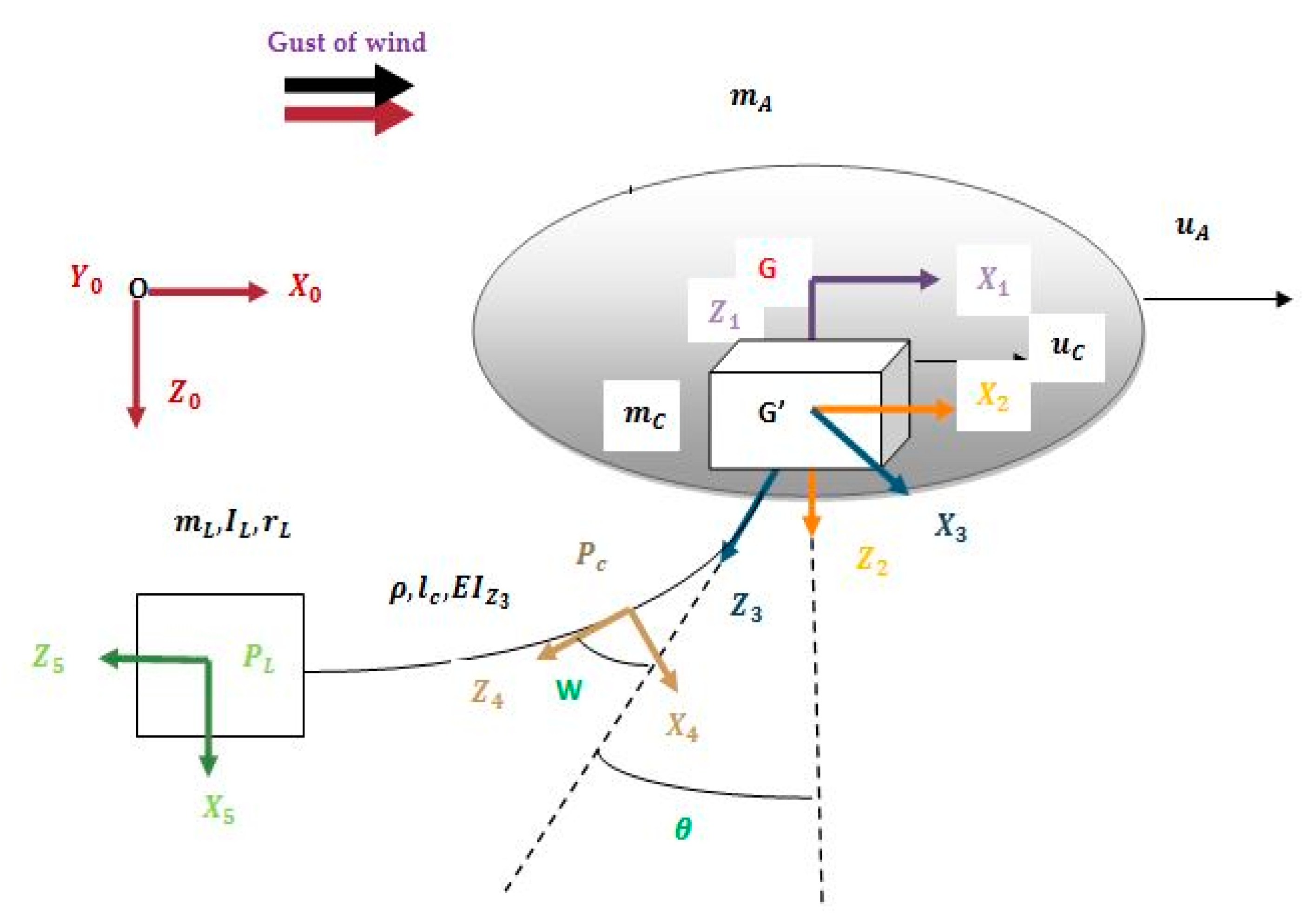
3.2. Dynamic Modeling of the Multibody System in a Plane Motion
As an application, we are interested in modeling the system assuming that the airship as well as the cuboid move in
XZ space. They follow unidirectional motion along axis (
GX1) and axis (
G’X2), respectively. The system to be modeled is shown in
Figure 9. It is composed of an airship, a cuboid, and a load suspended by a cable. The latter, which holds the container, is thick and massive. Unlike the cables that support the cuboid, we will consider here its flexibility as well as its elongation. The cable has a length
lc, a mass per unit of length
ρ, a modulus of Young
E, and a moment of inertia
Iy3. The load has mass
mL and matrix of inertia
IL. The distance between its center of mass and the end of the cable is represented by
rL, and the deformation is denoted by
ω.
As part of the modelling of this system, this assumption will be retained: the rotational inertia of the pulleys is neglected in front of the other inertias.
The analysis of the global system motion is made with respect to six reference frames, namely:
- i.
An earth-fixed frame .
- ii.
A local frame fixed to the airship , having as origin the inertia center of the airship.
- iii.
A local frame fixed to the cuboid , having as origin the inertia center of the cuboid .
- iv.
A reference frame , linked to the cable in rotation at an angle with respect to R2.
- v.
A reference frame , attached to any section of the cable located at a distance from the axis.
- vi.
A reference frame , at the end of the cable to describe the motion of the load.
To facilitate the writing of the equations of motion, we adopt the notations below: ,, , represent the deformation of the cable as well as its derivatives at a point of the cable.
When point
is equal to
, the deformation and its first and second derivatives are noted by:
In order to apply the Lagrange equations, we need to calculate the Lagrangian of the system. This Lagrangian can be defined as follows as in [
27]:
With Ttot is the total kinetic energy of the system, Vtot, is the total potential energy, and FR is the Rayleigh dissipation function.
3.2.1. Kinetic Energy of the System
It should be noted that the kinetic energy of the whole system is made up of that of the airship (
TA), the cuboid (
TC), the payload (
TL), and the flexible cable.
We will denote by uA and uC the speeds of the airship and of the cuboid projected onto the mobile reference frames linked to each of them. In our particular example of a plane case, we have: .
The kinetic energy of the airship is simply expressed as:
TC is the kinetic energy of the cuboid:
where
mC is the mass of the cuboid, and m
A is the mass of the airship including the added mass. For more details concerning the added masses one could consult [
28]. The kinetic energy of the load has two terms: the first term which takes into consideration the linear motion of the body with respect to the frame
R3 and the second term which takes into consideration the rotation of the load. The expression of the kinetic energy of the load is:
are small terms of the third order that can be neglected later.
On the other hand, the kinetic energy of the cable is computed by a summation over the entire length of the latter. We can see its expression in detail in
Appendix A.
By developing the equations of the kinetic energy of the cable and of the load, we will keep the expressions of the position and the speed exact to the second order. All other quantities can be linearized. Finally, to obtain the expression for the linearized total kinetic energy of the system, it would suffice to add and rearrange the corresponding terms. The developed expression of the total kinetic energy of the system can be seen in
Appendix A.
3.2.2. Potential Energy
The potential energy will be computed using the same reasoning as that of the kinetic energy: in theory, the potential energy of the multibody system is the sum of the potential energies of the different bodies.
However, for the case mentioned in
Section 3.2.1, and which will be our illustrative example in this paper, the airship as well as the cuboid will have horizontal rigid body motions and will therefore not affect the potential energy. For these reasons, the total potential energy can be written as:
The potential energy of the load is given by:
On the other hand, the potential energy of the cable will not only have the contribution of gravity but also a contribution given by its elasticity, which we could write as follows:
Hence the expression of the total potential energy becomes:
3.2.3. Dissipation Function
Within a flexible metal cable, there is an internal energy dissipative damping. To model this characteristic, the Rayleigh dissipation function was used. Its expression is:
In order to obtain a dynamic model having a reasonable number of degrees of freedom, modal synthesis will be used to discretize the energies calculated previously. This procedure is usual in the vibratory problems and allows the number of degrees of freedom to be minimized in our precise case by minimizing the modes retained. This will have the advantage of facilitating the implementation of control laws.
3.2.4. Modal Synthesis
The vibration of cables is extensively investigated in the literature. Recently, vibration of axially moving materials has received a great deal of attention in the literature (see, for example, [
29]). These survey papers present a picture of the state of the art in the vibration and dynamic stability of axially moving strings or beams. Little research on the vibration behavior of overhead cranes with flexible cables has been studied in [
30,
31]. In the study of [
32], the authors used the Rayleigh–Ritz discretization method. Meirovitch [
33] describes the behavior of the deformation of the cable as an ordinary differential equation model. Another approach named the Galerkin method has been used by a number of researchers to solve problems of deformation of cables of fixed length [
34]. Vibration problems of materials whose effective lengths vary with time have also been the subject of recent research activities where the system is discretized via a modified finite element technique [
35,
36], and finally a modified Galerkin method was used by Fung [
37].
In the present work, we have used the assumed modes method. This approach consists in representing the deformation as a weighted sum of the shape functions. The solution is approximated by a series of finite superimposed functions multiplied by indeterminate coefficients. In other words, this deformation is decomposed into two functions as in [
38]: a spatial function over the length of the cable
, and a time varying function
as follows:
where
is the vector of shape functions. This vector gives the general configuration of the cable,
is the vector of the generalized coordinates relating to the flexible modes. This vector represents the nature of the motion made by the cable and m being the number of modes retained in the series.
By replacing the expression of the deformation defined above in that of kinetic energy, we obtain a new developed expression of the kinetic energy (see
Appendix B).
This expression can be written in the following compact form:
Let us denote by:
the mass matrix;
the damping matrix;
the stiffness matrix;
the vector of forces due to the gravity;
the vector of Coriolis and centrifugal forces;
the vector of the forces produced by the actuators and applied on the airship and on the cuboid. (The details of these matrices are given in Appendixes B–D).
Using the same procedure as that developed in the discretization of kinetic energy, the expression of the discretized potential energy is given by:
The discretized potential energy of the system can be rewritten in a more compact form such as:
The discretized Rayleigh function can be written in the form:
In matrix form, it will be written as follows:
3.2.5. Equations of Motion
Once the energies have been discretized as well as the Rayleigh function we obtain a discretized Lagrangian L (Equation (6)) to which we apply the Lagrange equations:
The dynamics of the system can be written in compact form in terms of the generalized coordinates
:
3.2.6. Simplified Model
The model of the multibody system developed above corresponds to a nonlinear system fully coupled to (m + 2) states. In order to remedy the complexity of the model, we have made some simplifications and arrived at a reduced and simplified model.
- (a)
The first simplification concerns the shape functions: we have chosen the shape functions
and we have taken only one mode (m = 1), the expression of the deformation then becomes:
- (b)
With the aim of simplifying the dynamic model in order to be able to apply control laws to it, we have analyzed the different terms of the matrix
and succeeded in highlighting the terms whose calculation is complex, but whose absolute value can be neglected compared to the other terms of the matrix. The mass matrix
can thus be subdivided as the sum of two matrices: main matrix noted
and complementary matrix
:
The expressions of matrices
and
are defined in
Appendix D. We note that matrix
consists of small terms compared to those of the main matrix. These terms will be neglected in continuation and consequently, we can suppose that
.
- (c)
A third simplification is carried out for the Coriolis vector. We replace
with
in Equation (A24) (see
Appendix D) and thus obtain the following expression of
:
The new Coriolis vector will be:
with
Remark 1. It should be specified here that this study is established for a given length of cable lc. During the loading or unloading phase, this length will vary. Because of the sensors at the level of the pulleys, the controller intended to stabilize the load will be able to know this length at time t and will take this information into account in real time.
3.3. Stabilization
The main objective of the design of this smart crane is to develop a control vector based on the various actuators of the system to stabilize the airship and its load during the loading or unloading phase. As a first approach, we present a classic system based on the Proportional-Derivative (PD) technique. Stabilization by the qLPV method and by model-free control will be presented in future work.
The proposed PD control law is based on measurable variables for the airship and the cuboid, namely the displacement and speed of the airship and the cuboid, the oscillation angle and its angular speed, and the deformation of the cable and its speed.
Different scenarios were considered and simulated numerically in order to validate our mathematical model.
4. Simulation Results
The numerical simulations presented in this section concern the most feared scenario of a gust of wind impacting the airship during the loading or unloading phase. A controller is proposed to drive the system to a stabilized position and at the same time minimize the cable oscillations in order to preserve the products loaded in the container. The main control objective is to use the cuboid acceleration to stabilize the motion of the cable while damping the cable vibrations. The various computer developments were carried out within the Matlab software R2022a.
The actuators available are, on the one side, the motorized pulleys which pull the eight upper cables in order to control the motion of the cuboid and, on the other side, the thrusters which act on a longer timescale in order to stabilize the airship.
In these simulations, the characteristics of the different elements of the system (airship-cuboid-load and flexible cable) are listed in
Table 1:
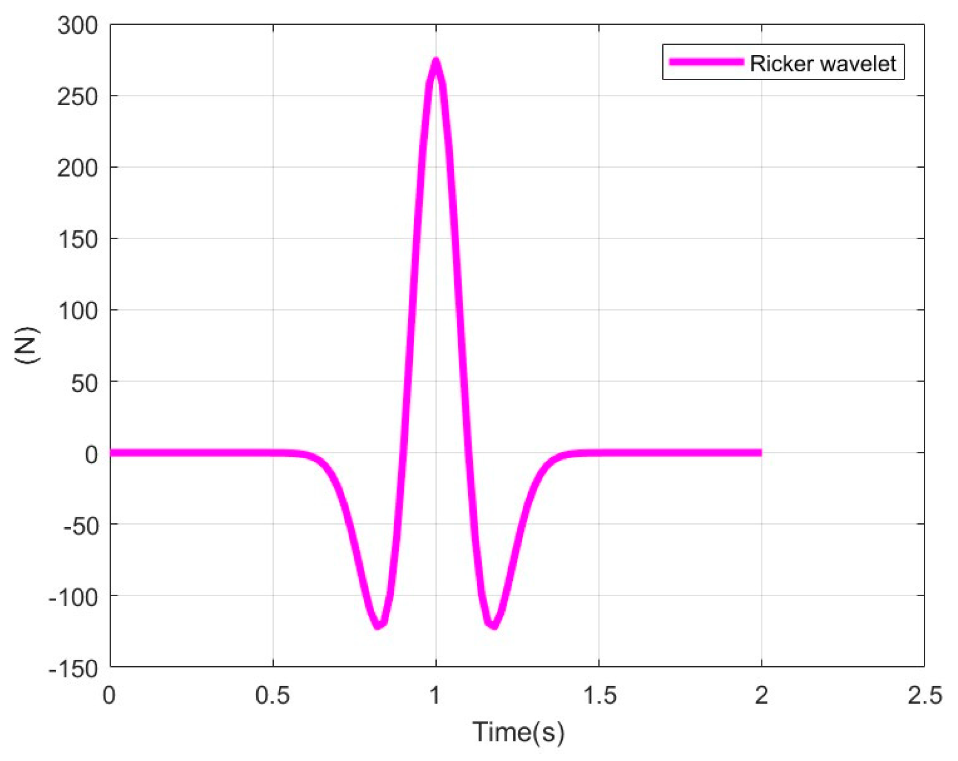
We have assumed that the airship is subjected to a gust of wind which will be represented by a Ricker wavelet along the
X1 axis as we can see in
Figure 10:
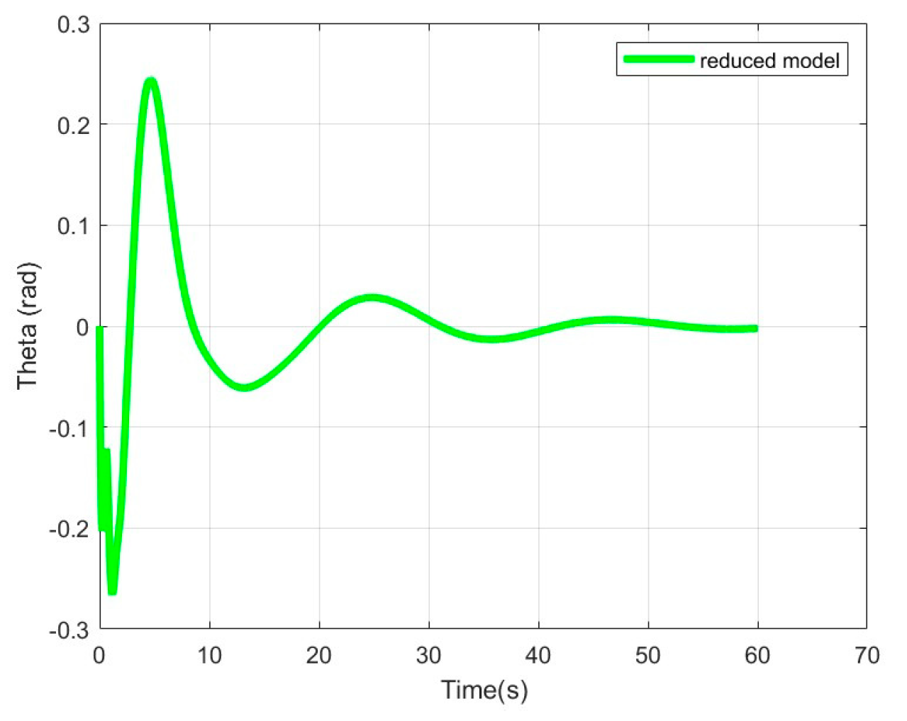
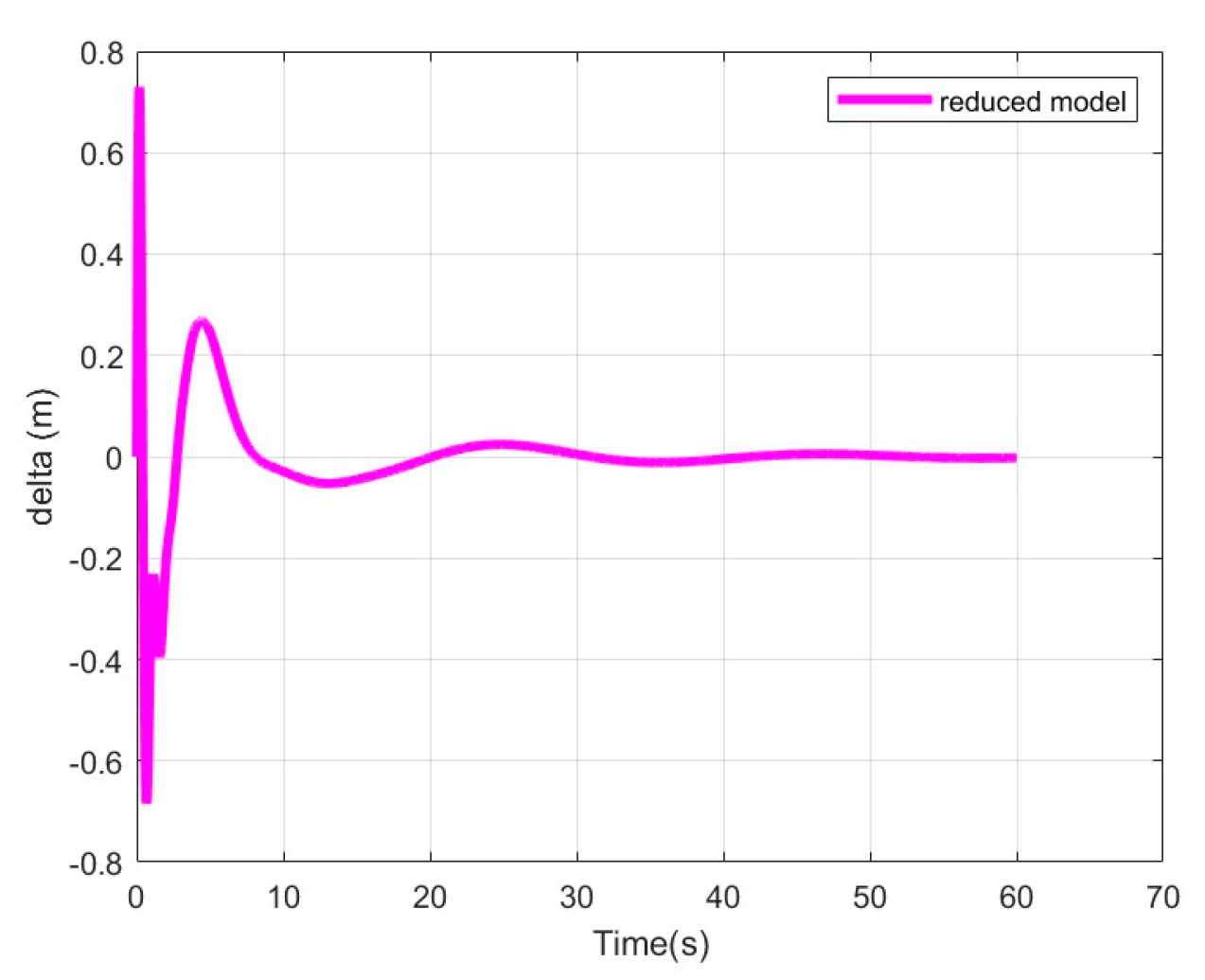
During our simulations, we found that the difference in response between the complete model and the reduced model is less than 1%. The different curves are superimposed perfectly, which justifies the reduction of the model that we have made and which allows a notable reduction of time in the simulation in comparison with the complete model. We have therefore chosen to present the curves of the different variables calculated from the reduced model.
We notice also that under the effect of this impulse caused by the gust of wind, the system oscillate due to the inertial coupling between the various generalized coordinates (displacement of the airship xA, displacement of the cuboid xC, oscillation and deformation of the cable θ and δ).
We apply a control vector which acts, on the one hand on the airship, through force
developed by the thrusters along axis
in order to stabilize the latter around a desired position
and, on the other hand, on the cuboid by force
along axis
produced by the eight winches which drive the cuboid, such as:
Unlike agile flying machines such as helicopters, the dynamics of the airship are slow dynamics. This is what motivated our choice to stabilize the suspended load by the acceleration of the cuboid, which benefits from the advantages of the CDPM and therefore has a quick dynamic.
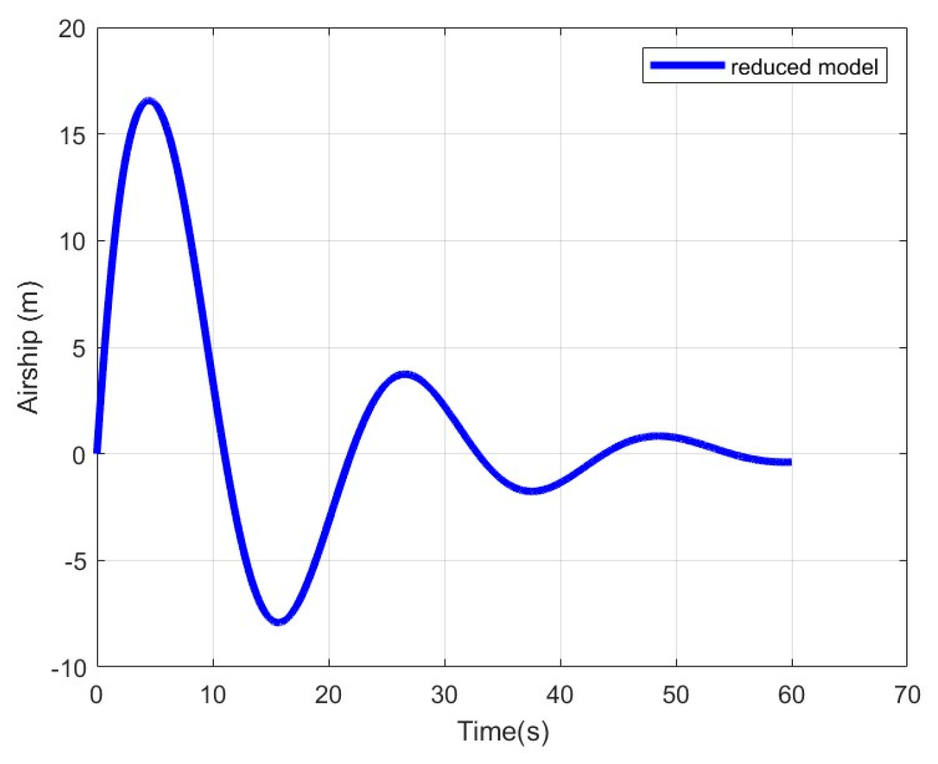
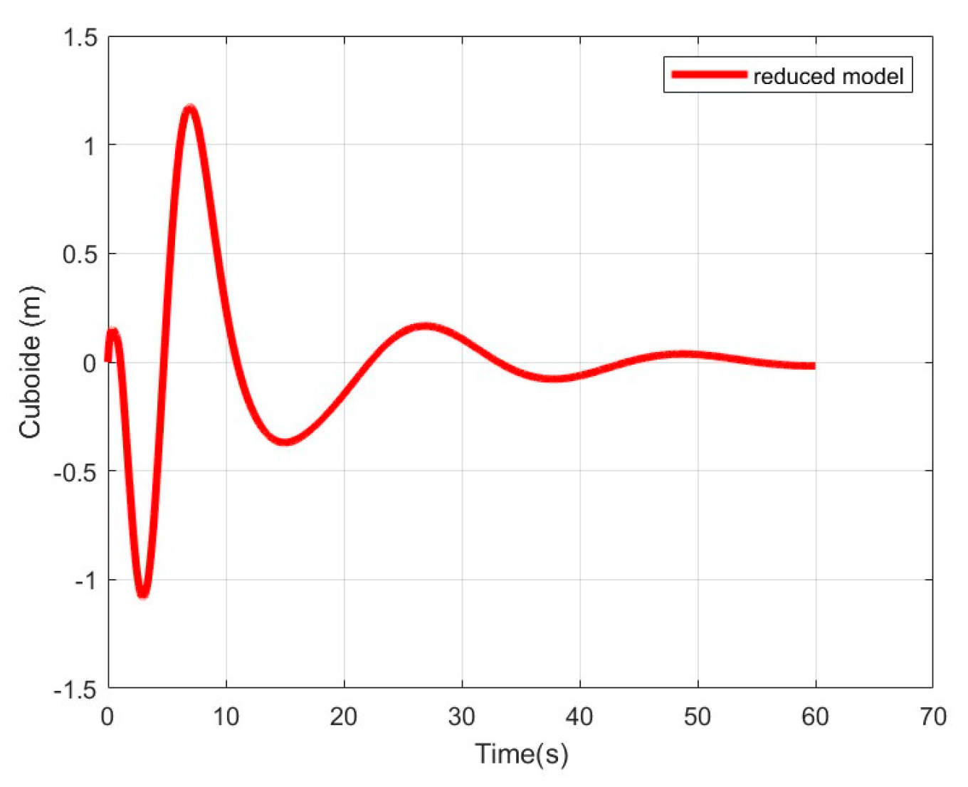
According to
Figure 11, the airship reaches slowly the desired position (origin). The control vector succeeds in stabilizing the system. The motion of the cuboid, the oscillation angle
θ, and the generalized deformation of the cable
δ tend to zero.(
Figure 12,
Figure 13 and
Figure 14).
We can see that the proposed PD-type closed loop control system reasonably suppresses the load oscillation, and it is also efficient at damping cable vibrations. In addition, the final positions of the airship and the cuboid are reached in a relatively reasonable time.
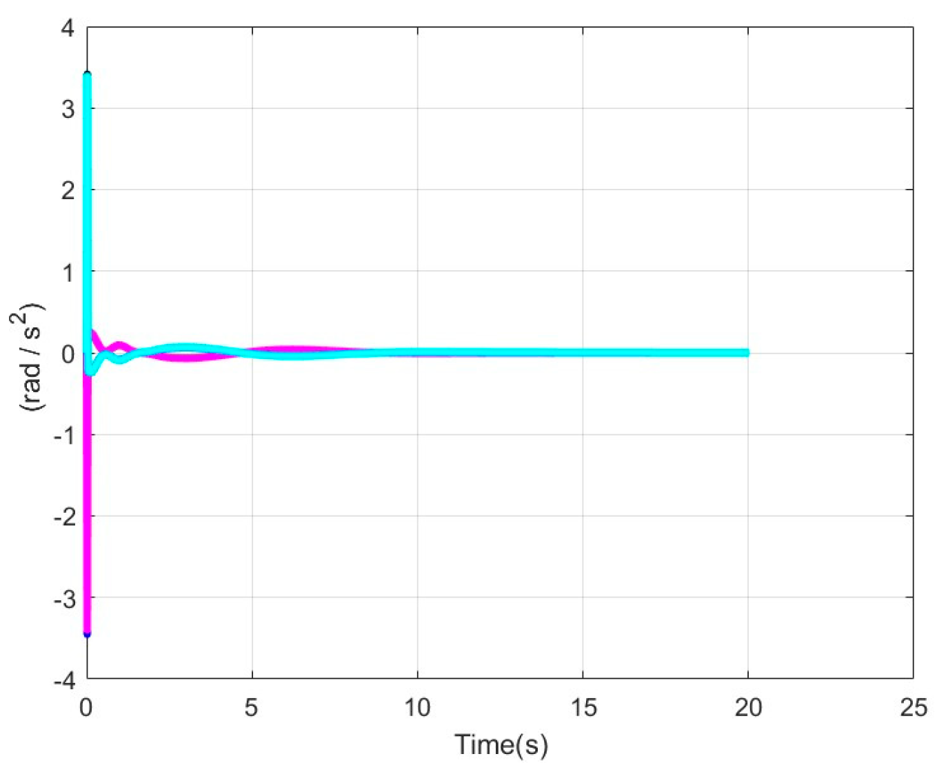
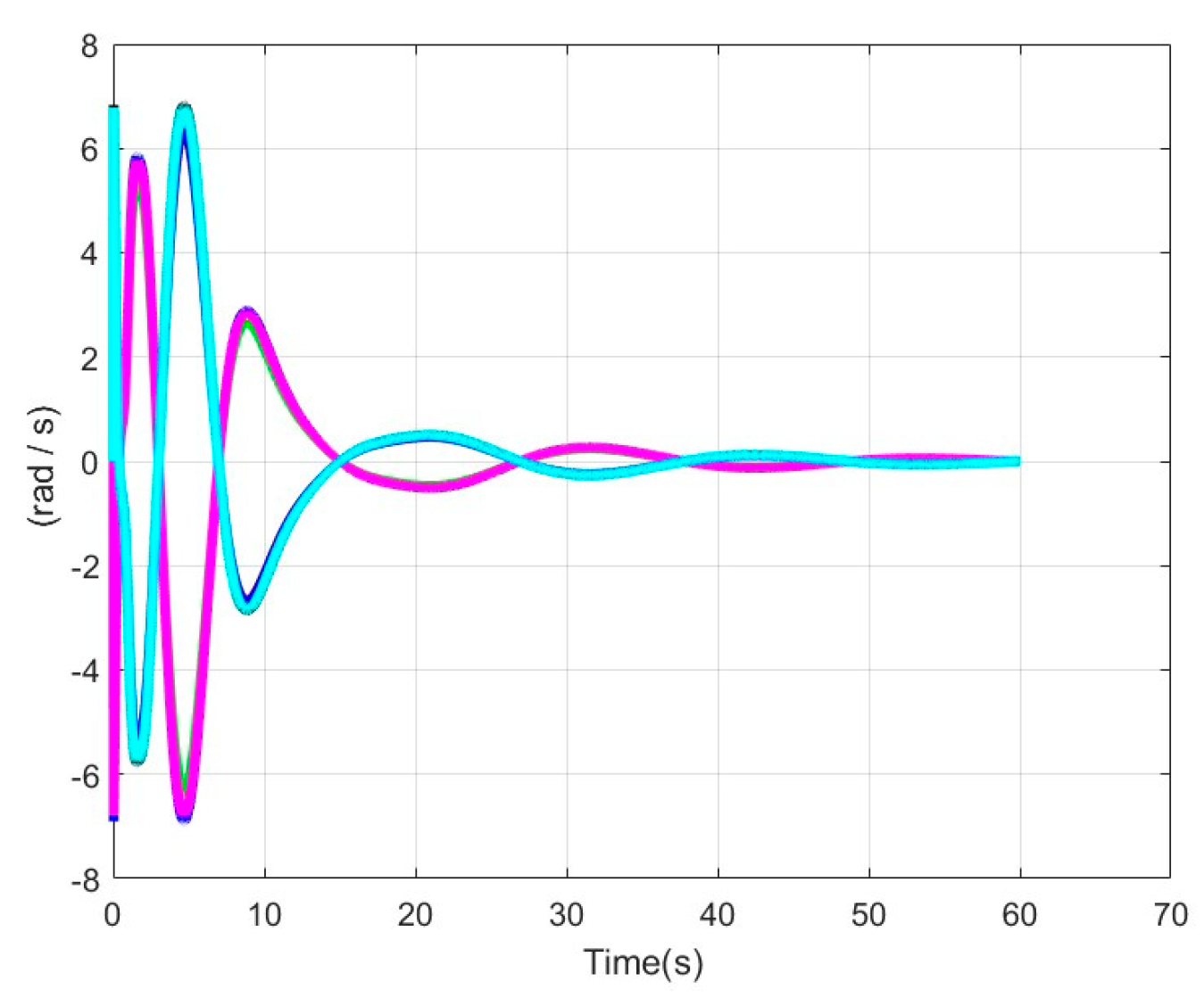
The performance of the proposed control scheme is good. Our goal thereafter is to highlight the behavior of the eight winches driving the cuboid. We show in
Figure 15 the detail of all the simulation of the accelerations of each winch.
We recall that the expression which links the cuboid accelerations with the angular accelerations
of the eight actuators is given by:
where
J is the Jacobian matrix of the robot.
The coordinates of the exit points and the attachment points used in this example are taken from a reference example given by the Tecnalia Company for an industrial CoGiRo robot. They are listed in
Table 2:
The diagonal matrix . The following figure shows the acceleration behavior of these eight actuators.
Figure 15 and
Figure 16 show the angular accelerations and speeds of the motorized pulleys which drive the cuboid. With the movement of the latter being rectilinear along axis
, it is noted that the accelerations of the “front” pulleys (colored in blue) are identical and opposite to those placed at the rear of the cuboid (colored in magenta).
5. Discussion
In this study we wanted to validate a concept. It involved equipping a Large Capacity Airship with a smart on-board crane capable of stabilizing the load, in addition to its usual functions of lifting the load and arranging the containers in the hold of the airship. By design, this innovative crane can stabilize the load regardless of the direction of oscillation. We have conducted an extensive study on the dynamics of the multibody system including the flexible heavy cable. However, in this study, we made a strong hypothesis and confined ourselves to a disturbance of the wind along the x axis alone. The results obtained are encouraging and allow us to validate the concept. We remain aware that the dynamic model used for the airship is relatively simplistic. Our first objective was to present the smart crane and its interaction with a particular movement of the airship.
Generalization to external disturbances along various directions and taking into account the complete dynamic model of the airship [
3] is being studied and will be the subject of future publications.
6. Conclusions
As part of the development of large capacity airships, we have presented in this paper the design and modelling of an on-board smart crane based on the CDPM principle. The main objective of this crane is to ensure safe handling at altitude, in particular for loading or unloading container ships on the high seas. For this objective, we have established a precise mathematical model of a multibody system including the airship, the crane, the flexible lifting cable, and the suspended load. For control requirements, we proposed a reduced dynamic model which proved to be very reliable and consistent with the complete model, while being very useful for control applications.
A classical control vector was applied to the system for its stabilization after a disturbance due to a gust of wind. The numerical results were conclusive and validated our model.
More elaborate control laws (qLPV control and modeless control) are under study and will be the subject of future publications.


