
A Review of Solution Stabilization Techniques for RANS CFD Solvers
by
 and
and
Shenren Xu
1,
Jiazi Zhao
1,
Hangkong Wu
1,
Sen Zhang
1,
Jens-Dominik Müller
2,
Huang Huang
1,
Mohammad Rahmati
3 and
Dingxi Wang
1,* 1
Northwestern Polytechnical University, Xi’an 710072, China
2
Queen Mary University of London, London E1 4NS, UK
3
Northumbria University, Newcastle upon Tyne NE1 8ST, UK
*
Author to whom correspondence should be addressed.
Aerospace 2023, 10(3), 230; https://doi.org/10.3390/aerospace10030230
Submission received: 6 November 2022
/
Revised: 18 February 2023
/
Accepted: 20 February 2023
/
Published: 26 February 2023
(This article belongs to the Special Issue Adjoint Method for Aerodynamic Design and Other Applications in CFD)
Abstract
:Nonlinear, time-linearized and adjoint Reynolds-averaged Navier-Stokes (RANS) computational fluid dynamics (CFD) solvers are widely used to assess and improve the aerodynamic and aeroelastic performance of aircrafts and turbomachines. While RANS CFD solver technologies are relatively mature for applications at design conditions where the flow is benign, their use in off-design conditions, featuring flow instabilities, such as separations and shock wave/boundary layer interactions, still faces many challenges, with tight residual convergence being a major difficulty. To cope with this, several solver stabilization techniques have been proposed. However, a systematic and comparative study of these techniques has not been reported, to some extent hindering the wide deployment of these methods for industrial applications. In this paper, we critically review the existing methods for solver convergence stabilization, with the main purpose of explaining the rationale behind the algorithms and providing a systematic view of the seemingly different methods. Specifically, mathematical formulations and implementation details of these methods, example applications, and the pros and cons of the methods are discussed in detail, along with suggestions for further improvements. This review is expected to give CFD method developers an overview of the various solution stabilization methods and application engineers an idea how to choose a suitable method for their respective applications.
1. Introduction
Computational fluid dynamics (CFD) solvers based on the Reynolds-averaged Navier-Stokes (RANS) equations are now indispensable for aircraft and turbomachinery aerodynamic/aeroelastic design and optimizations [1,2]. Although RANS CFD solvers are relatively reliable at design conditions where the flow is benign, its use at off-design conditions for industrial applications, featuring flow instabilities due to shock wave/boundary layer interactions and complex secondary flows, still faces many challenges. Among them, robust residual convergence should be the first to be addressed [3] before other aspects are examined, such as grid independence, discretization consistency, and turbulence modeling applicability. The challenge of robust residual convergence is not only faced by nonlinear steady solvers but also by linearized ones, such as time-linearized solvers for aeroelasticity study [4,5], tangent-linearized and adjoint solvers for stability analysis [6,7,8], and adjoint solvers for shape optimizations [9,10,11].
Commercial aircraft typically cruise at transonic speeds, where shock wave/boundary layer interactions pose a great challenge for RANS CFD-based aerodynamic and aeroelasticity analyses. In addition, off-design flight conditions, such as take-off, landing, and maneuvers, are frequently characterized by complex flows, particularly large regions of separated flows, and this is often associated with complex geometries. As for turbomachinery components, such as compressors and turbines, they are now designed with increasingly higher loadings, characterized by flows more prone to separations. Similar to commercial aircraft, turbomachinery components also have stringent demands for off-design performance, where the flow is even more complex and unstable. These challenges in aircraft and turbomachinery designs require nonlinear and linearized RANS solvers that are robust (here robustness refers to the ability to achieve deep residual convergence) in the presence of complex flows and geometries. Compared with nonlinear flow analyses, which are sometimes tolerant to not fully converged solutions, as partially or oscillatorily converged flow solutions, can still be of use for engineering purposes, and linearized solvers are much more delicate, as they can either fully converge or diverge, due to their linear nature. When a linearized solver fails to converge, the linear analysis process would terminate. Even for nonlinear flow analyses, if the ultimate goal is to perform stability analysis, then a stringent residual convergence criterion is also highly desired.
To cope with the residual convergence difficulties of RANS solvers, several stabilization methods have been proposed over the past years, namely, the recursive projection method (RPM) [12], the selective frequency damping method [13], the BoostConv method [14], as well as Newton’s method, and other implicit methods [15,16,17]. Although these stabilization methods are proposed independently in different contexts, there exist a great deal of commonalities in their underlying principles. A thorough and critical review of these seemingly different methods would allow readers to better understand the underlying stabilization mechanism and utilize these methods more effectively. However, no systematic review of these methods has been reported in the literature, which significantly hinders the wide deployment and further development of these methods. In this paper, a review of existing methods for stabilizing non-converging RANS CFD solvers is performed. Basic theories behind these methods are explained, followed by simple examples to illustrate their working principles. The pros and cons of the various stabilization approaches are discussed and illustrated with practical examples reported in the literature. Finally, suggestions for further development are made.
2. Theoretical Background
To explain the mechanism of the various convergence stabilization methods, it is useful to first discuss the convergence instability issues and their origins. Therefore, a brief introduction of the mathematical formulations of the nonlinear and various linearized RANS equation systems are first presented, followed by an in-depth discussion on their linear stability properties in relation to each other, utilizing a fixed-point iterative scheme, which explains the root cause of the instability issues. Although the linear stability analysis based on the fixed-point iterative scheme does not cover all failure modes when non-convergence occurs, it is believed that it still captures the essence of the stabilization mechanism of the methods discussed in this review, as they all tackle the linear stability of the underlying nonlinear and linear iterative schemes.
2.1. Time-Marching Nonlinear RANS Equation Systems
A nonlinear steady RANS CFD solver essentially seeks the root of the following nonlinear system of equations
where is the vector of design variables that uniquely defines the geometry, which in turn, via a deterministic meshing algorithm, determines the computational mesh, U is the flow solution vector, and R is the residual vector, which represents a particular spatial discretization scheme. R is a nonlinear function of U, and the discretization scheme uniquely determines the solution U to be found for a given geometry/mesh. A time-marching scheme via fixed-point iterations (FPI) for the discrete nonlinear flow equations can be expressed as
where and denote the approximate solution to the nonlinear flow Equation (1) at the nonlinear iteration and the solution increment, respectively. The matrix M represents a general time-stepping operator. Towards full convergence, the error between and the fully converged solution , denoted by , evolves as
which yields
where the matrix A is the exact Jacobian of the nonlinear residual vector with respect to the flow solution. Therefore, a necessary condition for the solution to fully converge is that the spectral radius of the matrix operator does not exceed unity. It should be noted that this is not a sufficient condition for full convergence. The first difficulty in obtaining a fully converged nonlinear flow solution is to overcome the strong initial transient and allow the solution to evolve towards the basin of attraction of the nonlinear operator , where such a stability analysis can be performed.
2.2. Time-Marching Linearized RANS Equation Systems
A RANS-equations based aerodynamic optimization problem can be expressed as
where J is the objective function of interest. U and are related through the nonlinear RANS Equation (1). The chain rule can be applied to obtain the gradient of the objective function with respect to the design variables
The matrix , denoted by u, satisfies the tangent-linearized flow equations
To obtain each column of the matrix u, a linear system of the following form needs to be solved
Further denoting by , then the tangent-linear solution based sensitivity calculation is
For a high-dimensional problem with N design variables, N large sparse linear systems of Equations (8) need to be solved, which would render the calculation of design sensitivities extremely computationally expensive. To circumvent this problem, the discrete adjoint approach can be used, where one solves the adjoint equation
with the vector v being the adjoint solution. It can be easily verified that
and thus the gradient of the objective function can be evaluated with the adjoint solution as
Different from the tangent-linear approach, computing the gradient using the adjoint approach only requires solving M large sparse linear system of equations with M being the dimension of J. Various other terms required to assemble the sensitivity vector corresponding to all design variables, i.e., and f, can be evaluated at a negligible cost. The overall computational cost for obtaining the design sensitivity vector is therefore almost independent of the number of design variables, making the adjoint method suitable for high-dimensional gradient-based aerodynamic optimization problems.
In the derivations above, the residual vector R represents the particular spatial discretization method and boundary conditions used in a given flow solver, and all the derivations are based on the already discretized system. The resulting method is thus called discrete adjoint [9,18]. Alternatively, one can also derive a continuous adjoint system, where one first analytically derives the partial differential equations for the adjoint problem using Lagrangian multiplier and then discretizes them [1,18,19]. A major advantage of the discrete adjoint approach is that the resulting gradient is consistent with the nonlinear flow calculations down to the machine precision [18]. Throughout the rest of the paper, all discussions on the stabilization of adjoint solvers are limited to the discrete adjoint approach.
An appealing property of the discrete adjoint equation is that its system matrix is the transpose of the primal flow Jacobian matrix A, hence having the same eigenvalue spectrum as the nonlinear and tangent-linear equations, as transposing a matrix does not alter its eigenvalues. This property can be exploited to analyze the convergence behavior of an FPI scheme combined with a given spatial discretization method. Applying the same time-stepping method to the solution of the tangent-linear and the adjoint equations leads to the following two discrete time-stepping schemes
and
The corresponding error equations, with and denoting the errors of the tangent-linear and the adjoint solutions, are
and
respectively. If the linearization and transposition are exact, the time-marching schemes of both the tangent-linear and adjoint systems have the same spectral radius as the nonlinear flow equations, since
where denotes the spectral radius of a matrix. Therefore, as long as the nonlinear flow solver is able to converge asymptotically, the corresponding tangent-linear and adjoint systems are bound to converge at the same rate. This is a powerful tool for developing and debugging a discrete adjoint and tangent-linear solver. On one hand, if the time-marching schemes for the tangent-linear and adjoint solvers exactly follow that of the nonlinear flow solver, convergence is guaranteed if the nonlinear flow solution converges asymptotically for the problems considered. On the other hand, when differences exist in their respective convergence behaviors, it implies that algorithmic inconsistencies are introduced and implementation details should be checked.
Besides the tangent-linear and adjoint equations, there is another type of linearized RANS equations, namely, the time-linearized one, also called the linear harmonic equations. The time-linearized RANS equations are of the following form
where the right-hand-side term is a complex vector representing a temporally periodic forcing term, , I is an identity matrix, and is the angular frequency of the periodic forcing. The forcing term could be due to either a prescribed structural motion in the case of flutter analysis or a periodic flow perturbation, e.g., due to the wake or potential flow perturbation of a neighboring blade row in turbomachinery applications. Similar to the nonlinear, tangent-linear, or adjoint equations, the time-linearized equations can also be solved using time-marching methods
with being the preconditioning matrix that controls the time-stepping. Similar to the preconditioning matrix M for the nonlinear and tangent-linear system, can be formed by augmenting it with a purely imaginary part as
Similarly, a necessary condition for the time-marched equation system to converge is that the matrix operator for the error equation needs to be contractive, i.e.,
However, different from the tangent-linear and adjoint systems, the spectral radius of the matrix operator of the time-linearized system is in general not equal to that of the nonlinear system, except in the limit that , and, therefore, an asymptotically converging FPI for the nonlinear flow solver does not guarantee that the time-linearized solver following the same time marching scheme would converge.
3. Stabilization Techniques
This section will review the existing techniques for stabilizing the nonlinear and linear flow solvers in detail. They are (i) recursive projection method (RPM), (ii) selective frequency damping (SFD) method, (iii) BoostConv method, (iv) Newton’s method, and (v) other implicit methods. For each method, the mathematical formulation is first discussed, followed by example problems from the literature to demonstrate its stabilization effect. The pros and cons of different methods are discussed to help users choose an appropriate method accordingly.
3.1. Recursive Projection Method (RPM)
RPM was initially proposed to stabilize general unstable FPI schemes [12]. It was originally used for bifurcation analysis, and was later applied to stabilize and accelerate the convergence towards steady-state solutions for aerodynamic analysis [20,21]. It has also been used to stabilize a time-linearized solver [5,22] and an adjoint solver [10].
3.1.1. Theory and Examples
We are concerned with the general FPI Formula (2), which represents an arbitrary time-marching based nonlinear or linear flow solver. It can be any time-marching scheme ranging from an explicit, implicit, to fully-implicit Newton’s method, denoted by M, combined with additional acceleration techniques, such as multigrid. Rearranging Equation (2) and linearizing the residual about the exact solution , which satisfies , yields the following error equation
with
Whether the FPI converges to the exact solution depends on the eigenvalues of the iteration matrix F [11,23,24]. A necessary condition for the FPI to asymptotically converge is that all eigenvalues should have a modulus no larger than unity. In other words, the matrix F should be contractive. The core idea of RPM is that a Newton step is applied to the error modes in the linear subspace spanned by the unstable eigenvectors, denoted by , and the original FPI is applied only to error modes in its orthogonal complementary subspace, denoted by .
Suppose that m eigenvalues lie outside the unit circle in the complex plane, that is,
the linear subspace is therefore spanned by the corresponding m eigenvectors . Define the orthogonal projectors P and Q onto the two subspaces and as
where is an orthonormal basis of , which can be computed by applying the Gram-Schmidt orthogonalization on the unstable eigenvectors . By definition, holds. Any can be uniquely decomposed as
where
are the projection of x in the subspaces and . For a preconditioned linear problem
decomposing the operator as yields
which can be used to construct an FPI as
Define the projection of both sides of the equation to subspaces and as
and
As mentioned above, the original FPI is applied to time march
It can be proved that for a fixed , the iteration for can stably converge. However, for , due to the outlier eigenvalues, applying the same FPI will lead to divergence. Instead, a Newton iteration is constructed by linearizing both sides of Equation (31) as follows
The resulting Newton iterative scheme for then becomes
It can be verified that
since
and the Newton update scheme for therefore becomes
where the low-dimensional matrix H is defined as
To compute the matrix H, is first computed via residual evaluations, and the m unstable eigenmodes are identified and orthonormalized to obtain V. The linear operator F is then applied to each column vector of V to obtain , whose m vectors are left multiplied with , at the cost of vector-vector multiplications, to obtain H. For nonlinear problems, if explicitly forming the linearized operator A is inconvenient, e.g., when only the outcome of one application of is exposed to the user and the source code for evaluating is hidden, then the matrix-vector product , where denotes the i-th vector of V, can be approximated using differencing, i.e., , for .
In the derivation above, a key step is to identify the unstable eigenvectors, which are used to form V. This is done by storing the last two solution incremental vectors, i.e., , when the iteration starts diverging. The two vectors are used to compute the Gram-Schmidt factorization
If , the dominant eigenmode is real and only the first column of is appended to V. Otherwise, the instability is caused by a complex conjugate pair, and both columns of are included in V. In contrast to this divide-and-conquer approach, alternatively, one could store more than two solution incremental vectors, and identify more unstable modes at a time by scrutinizing the T matrix. The latter results in a higher memory overhead, but usually with a stronger stabilization and acceleration effect.
To illustrate the RPM stabilization technique better, it is demonstrated on a simple linear problem test case. Suppose the linear problem to be solved is of the form
with the matrix A and the right-hand-side term b being
The linear problem is preconditioned with a Jacobi matrix M defined as
which imitates the effect of a local time-stepping approach commonly used in explicit flow solvers to accelerate the convergence. A FPI in the following form can therefore be constructed to iterate the equation to its solution
with the system matrix being
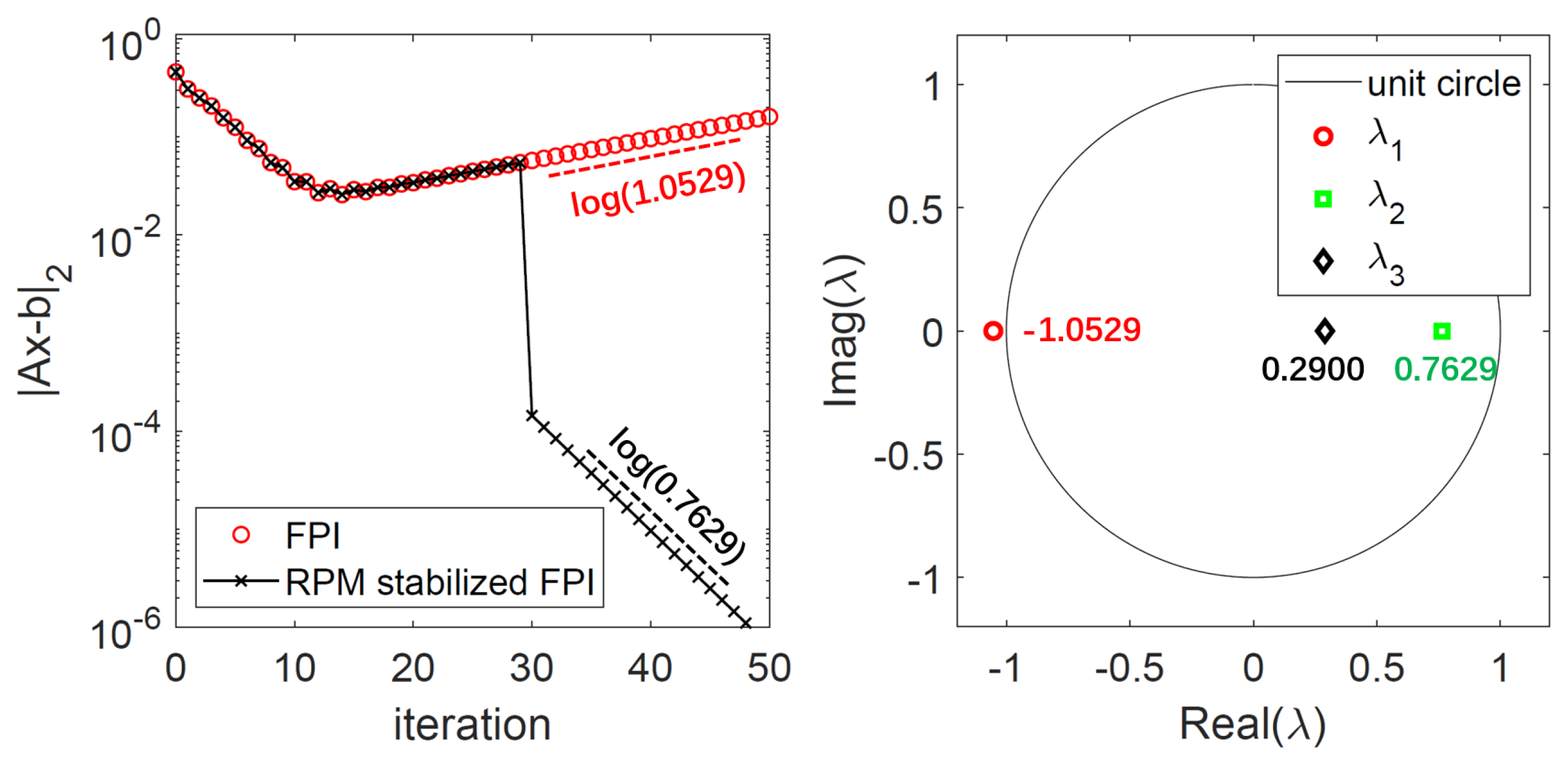
The eigenvalues of the matrix F are , and , respectively. Therefore, the FPI is unstable and is expected to diverge at the asymptotic rate of log(1.0529). This is confirmed via a numerical experiment as shown in Figure 1, with an initial value of . The choice of the initial solution does not alter the stability of the FPI, and the particular values are chosen only to produce a first-converge-then-diverge convergence history. Taking the only unstable eigenvector of as V, and activating RPM stabilization from the 31st iteration, the originally unstable FPI is stabilized, and the residual converges at the asymptotic rate of log(0.7629), also shown in Figure 1.
3.1.2. Rpm Stabilized Time-Linearized Analysis
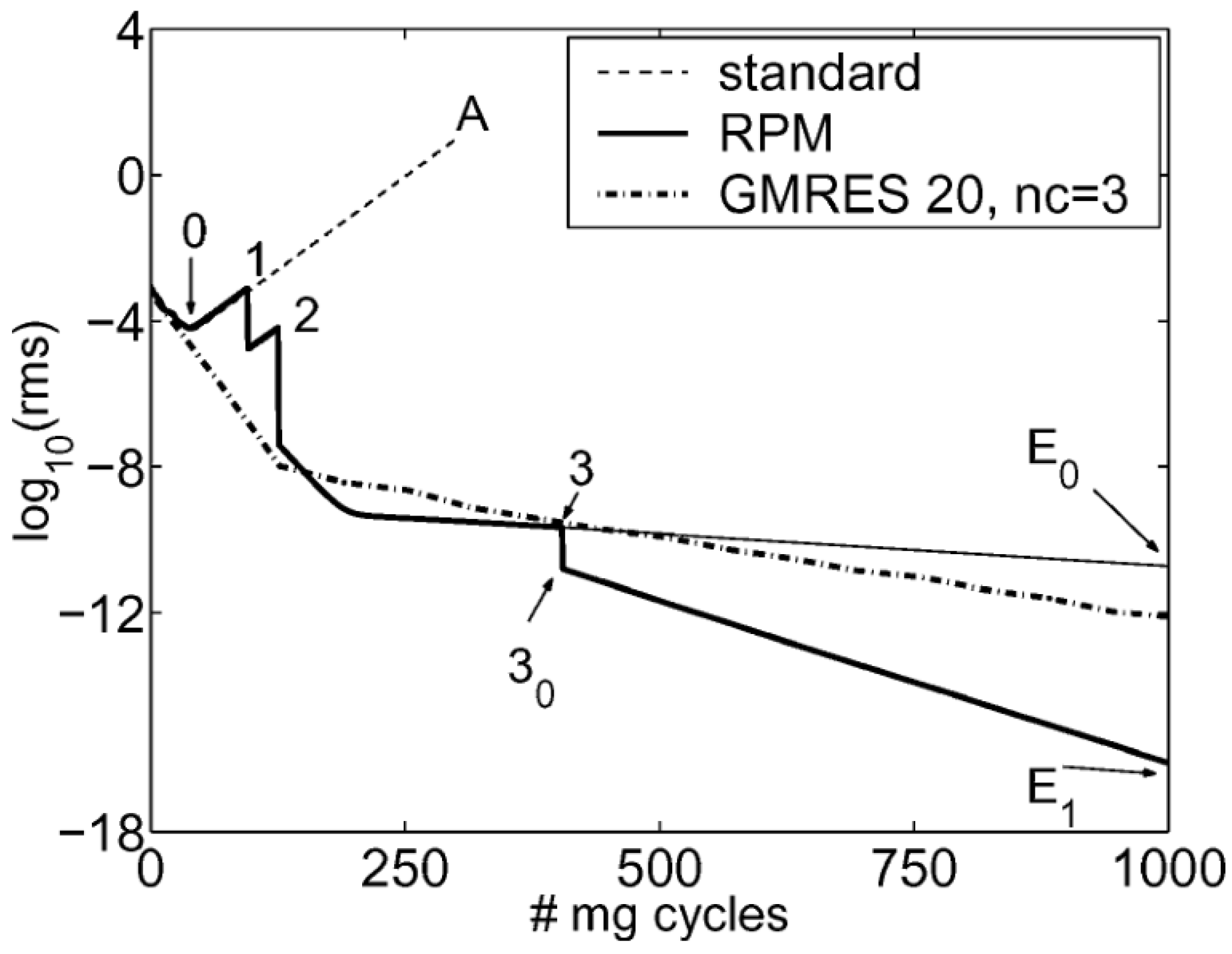
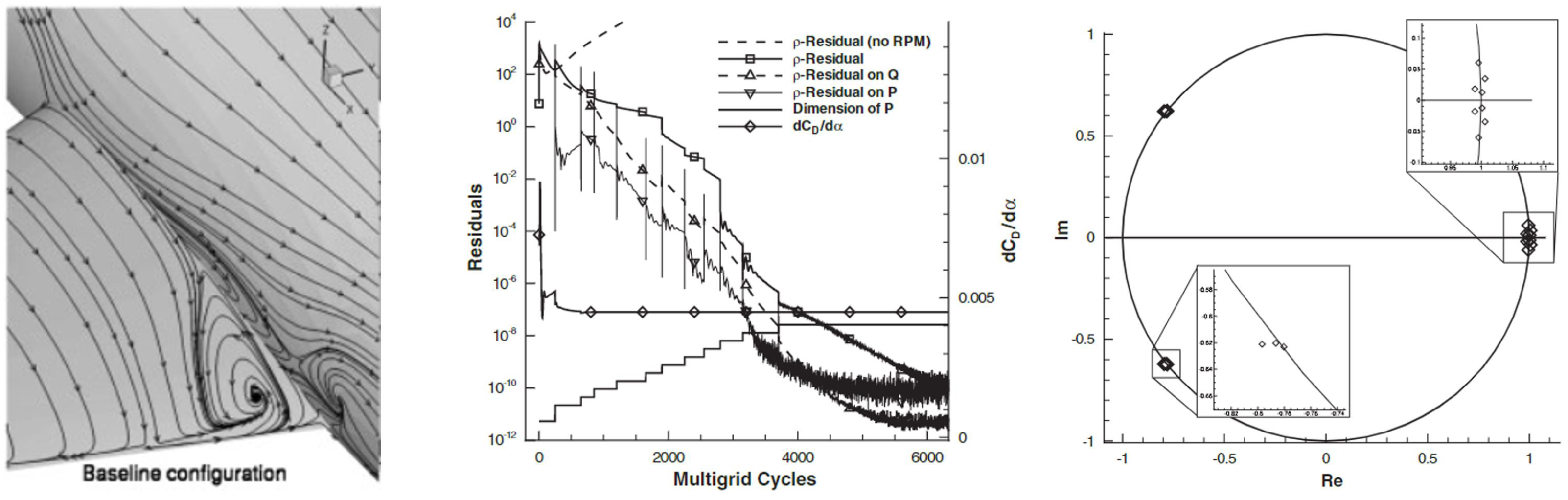
RPM was used to stabilize a time-linearized solver in [5], where a time-linearized (also called linear-frequency-domain or linear-harmonic) solver is used to compute the frequency-domain unsteady flow around a two-dimensional turbine section. The calculations of the steady base flow at both the subsonic and transonic conditions converged without difficulties to machine precision. The Mach number contours of the converged transonic base flow solution are shown in Figure 2, where a separation bubble on the suction side near the leading edge can be seen. For the transonic condition, the time-linearized analysis diverged exponentially with the standard linear code that uses the same time-stepping scheme as the nonlinear solver, and the convergence history (with the legend ’standard’) is shown in Figure 3. As discussed, the spectral radius of the time-marched time-linearized system is different from that of the nonlinear system, due to an additional purely imaginary diagonal term, and thus the asymptotic convergence of the nonlinear solver does not guarantee that of the time-linearized one. The convergence of the time-linearized solver is stabilized by applying RPM to the original FPI. In RPM, applying the Arnoldi procedure to the diverging iterative process allows the user to identify and extract the unstable eigenvalues and associated eigenvectors that are responsible for the divergence of the linear analysis. Additionally, shown in Figure 3 is the convergence history stabilized with generalized minimal residual (GMRES) preconditioned by multigrid. Further details on using GMRES for stabilization are discussed in Section 3.4. The least stable part of the full eigenspectrum is shown in Figure 4, where two pairs of conjugate complex eigenvalues that lie outside the unit circle are identified and believed to have caused the exponential divergence of the linear solver. First, the modulus of the eigenvalues farthest away from the origin is found to agree well with the rate of divergence, indicating the correctness of the eigenvalue analysis. Second, the two unstable eigenmodes are visualized and found to correlate to the separation bubble shown in Figure 2.
The convergence history of the RPM stabilized FPI is shown in Figure 3, where discontinuities in the slope of the convergence history using the RPM solver labeled with 1, 2, and 3 mark the iterations at which the complex conjugate eigenpairs 1, 2, and 3 are appended to the subspace of the RPM procedure. It can be seen that as soon as the two unstable eigenpairs are included (from the point labeled with 2 in Figure 3), divergence is avoided immediately. Adding the third least stable mode (corresponding the point labeled 3 in Figure 3) to the subspace has the effect of accelerating the convergence, as expected from the theory.
3.1.3. Rpm Stabilized Adjoint Analysis
RPM was used to stabilize an adjoint solver based on the compressible RANS equations in [10] on two cases, namely, (i) the RAE2822 aerofoil case 10 (Reynolds number , Mach number , angle of attack ), and (ii) the DLR-F6 wing-body configuration (Reynolds number , far-field Mach number , angle of attack for a lift coefficient of ).
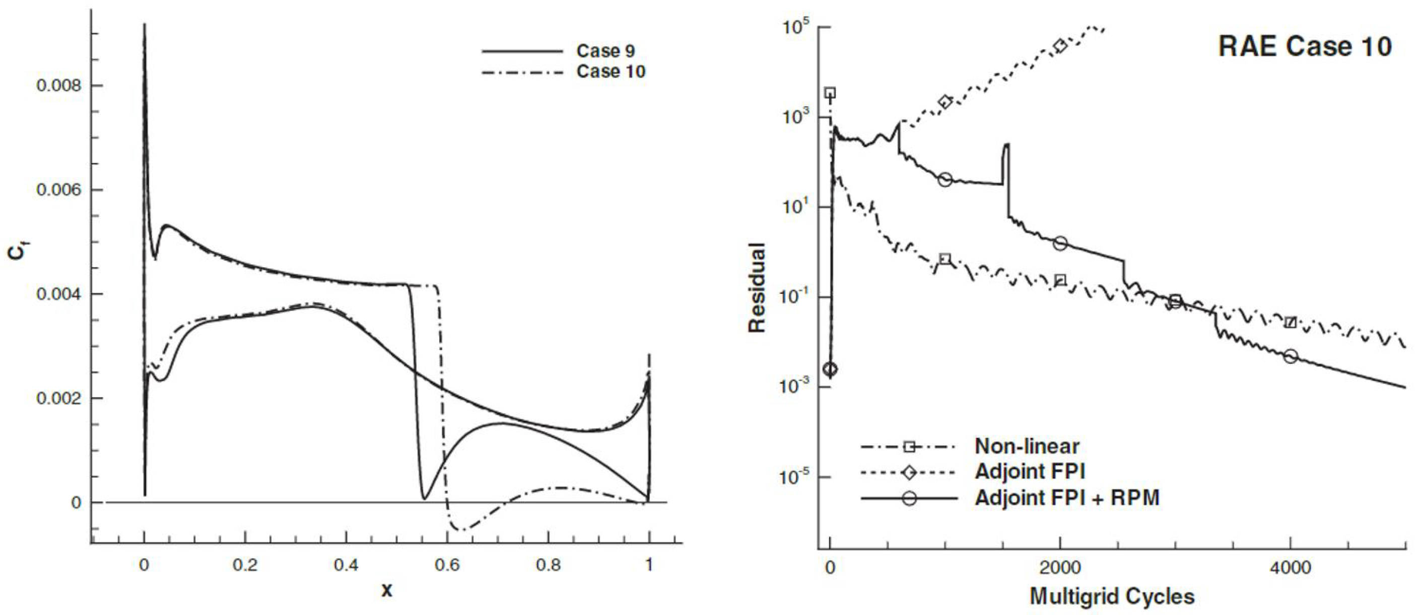
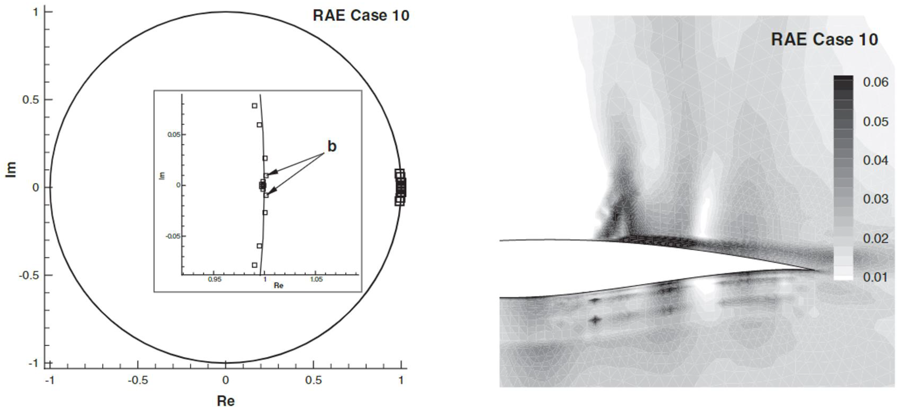
For the RAE2822 aerofoil case at the condition under investigation, there is a large region with shock-induced separation near the trailing edge, as indicated by the skin friction coefficient plotted along the chord on the left in Figure 5 (case 10). For this case, the nonlinear solver using lower upper symmetric Gauss Seidel (LU-SGS) as the smoother and accelerated using multigrid, failed to fully converge, and converged into a limit cycle instead. The adjoint solver following the same FPI scheme exponentially diverged, as shown on the right in Figure 5. Using RPM, the adjoint iteration is stabilized. The least stable eigenvalues can be identified in RPM and are shown in Figure 6. It can be seen that two conjugate complex eigenpairs exist, and the eigenvector corresponding to the most unstable ones, marked b, is visualized on the right in Figure 6. It can be seen that the unstable eigenvector strongly correlates with the shock-induced boundary–layer separation phenomenon.
For the DLR-F6 wing-body configuration, the nonlinear calculation is believed to have converged sufficiently to meet the engineering accuracy requirement. Although no details were given in [10], it is suspected that asymptotic convergence was not achieved with the nonlinear flow solver. The adjoint problem solved with LU-SGS or Runge-Kutta smoothed multigrid was found to be unconditionally unstable. Without discussing in detail whether this was due to the lack of asymptotic convergence of the nonlinear flow calculation, or the discrepancy in the spatial discretization between the nonlinear flow and the adjoint problem (as a frozen-eddy-viscosity approach was adopted for the adjoint solver for this case), RPM was used to stabilize the diverging adjoint solver in [10]. Phenomenologically, the divergence of the adjoint problem was believed to be related to the wing-body junction separation, as shown on the left in Figure 7. A numerical investigation of the dominant eigenvalues more rigorously identified the reason for the linear instability of the FPI for the adjoint problem. Four conjugate complex eigenpairs can be found in the approximate eigenspectrum, as shown on the right in Figure 7, which are believed to have caused the exponential divergence of the FPI without RPM. With RPM, once the eigenvalue outliers are included in the subspace , full convergence was recovered for the adjoint solver, as shown in the middle in Figure 7.
3.1.4. Rpm Accelerated RANS Nonlinear and Linear Calculations
Since RPM gradually removes the least unstable eigenvalues from the eigenspectrum of the FPI, which essentially reduces its spectral radius, it does not only stabilize the unstable FPI for linear problems, but can also accelerate the already-stable FPIs. This was successfully demonstrated in [10] for RAE2822 aerofoil at a condition where both the nonlinear and adjoint analyses were already stable using the baseline FPI. Using RPM, a typical speedup of 1.5 to 4 times in terms of CPU time was achieved, depending on the case and the required convergence criteria. When applied to the flutter analysis using a time-linearized solver for a two-dimensional turbine cascade case at a subsonic case, the convergence speedup in terms of CPU time by a factor of 2 to 3 was achieved. Further applications of the RPM to the acceleration of nonlinear flow solvers are discussed thoroughly in [20].
3.1.5. Summary of Current Status and Direction for Further Development
RPM has been successfully used for either convergence acceleration or stabilization of nonlinear and linear solvers for both external and internal flow problems. Its advantage is that it can be implemented in a non-intrusive way, only requiring the solution increment of each FPI step to be available to extract the unstable eigenvectors and build the subspace . One downside of the RPM technique is that it requires additional computation to build the Arnoldi subspace so that unstable modes can be identified and extracted. Building an Arnoldi subspace sufficiently large so that unstable modes can be identified accurately incurs additional computational and memory overhead, which can be significantly high if the number of unstable modes is large and/or the eigenvalue outliers are closely spaced.
To circumvent the weakness, an alternative criterion to select the unstable eigenmodes is proposed in [25]. The proposed criterion, based on an approximate eigenvalue problem (AEP), uses both the residual norm of the eigenpair and the modulus of the eigenvalues to identify the unstable subspace. It is able to select more eigenmodes per RPM iteration at lower memory and CPU time costs compared to the original criterion. It was shown for a transonic flow in a two-dimensional duct with a bump that the proposed AEP criterion achieves 14% to 67% speedup in terms of CPU time compared to the original Krylov criterion. A similar approach was proposed in [26], where the eigenvalues are identified approximately using the proper orthogonal decomposition (POD) approach. It was applied to the stabilization of a nonlinear solver for a two-dimensional turbine cascade in a viscous flow and a cascade of aerofoils in a transonic flow that resembles a modern fan-blade tip-section. For both cases, the original FPI scheme converged into a limit cycle. However, no comparison of the proposed POD-stabilized method against the original RPM or the improved version using AEP as the mode-selection criterion was conducted in [26].
Despite the various algorithmic improvements to enhance its computational efficiency and convergence robustness, the application of RPM to a practical three-dimensional cases with complex geometries and at challenging flow conditions still incurs a computational cost and memory overhead. The difficulty in finding unstable modes is further increased when RPM is applied to nonlinear flow solver stabilization, since the underlying flow Jacobian is varying over the iterations. Although RPM has been shown to be useful for stabilizing a nonlinear solver [26], it is believed by the authors that the success can largely be attributed to the fact the unsteadiness is sufficiently small, and thus the Jacobians nearly remain constant, since in the presence of the limit cycle nonlinear solver convergence, and, therefore, the unstable modes can be identified with a small number of solution snapshots. The main criteria to assess the effectiveness of RPM stabilization is the minimal number of solution snapshots required for the stabilization to take effect. When this number is large, RPM essentially approaches a direct solver, and its advantage of being a lightweight stabilization algorithm diminishes. In that case, it is probably more beneficial to use an implicit or even Newton’s method for stabilization.
3.2. Selective Frequency Damping (SFD) Method
The selective frequency damping (SFD) method was originally developed to obtain a steady base flow for the Navier–Stokes equations for globally unstable flows in the context of instability studies and flow control [13]. For such globally unstable flows, time-marching methods have difficulties in fully converging to steady solutions and instead often converge to limit cycles. Although a majority of existing work on SFD focused on the stabilization of nonlinear flow solvers, same as RPM, it is equally applicable to linear analyses, such as adjoint and time-linearized problems. In this subsection, the theory and the mathematical rationale behind the SFD method are first explained, followed by a review of a few typical application examples of the method in stabilizing nonlinear steady-state flow solutions. Finally, the pros and cons of the method are discussed, and suggestions for future work are proposed.
3.2.1. Theory and Examples
Similar to RPM, the SFD method is motivated by the observation that when the time-marched steady nonlinear flow calculation fails to converge asymptotically, it is often found to converge to a limit cycle, indicative of unstable modes in the underlying eigenvalue spectra. Different from RPM, which identifies the unstable modes and stabilizes their iterative update scheme by applying the Newton’s method, SFD tackles the oscillatory convergence that exhibits a marked characteristic temporal scale from a signal-filtering perspective. Assuming a fully-converged steady-state solution exists, denoted by , then it is possible to add a forcing term based on the deviation of the time-dependent solution from some time-averaged solution to the time-marching formula as feedback to the original unstable dynamic system. The modified dynamic system is
where represents a scaling factor prescribed by the user. Since the steady solution is not known a priori. In the SFD method, the reference solution in the forcing term is therefore based on a low-pass time-filtered solution. For a continuous function , the low-pass time-filtered signal is
where T is the filter kernel function and is the filter width. The exponential kernel defined as
is used. Using the integral form of the low-pass filter in expression (47) would require the entire flow solution history to be available and incur a high memory overhead and computational cost. Therefore, the integral form is differentiated with respect to time, and the following equivalent differential form is used in practice
In practice, the two systems (46) and (49) are time marched simultaneously. It can be shown that, although the operator of the original system is unstable, the operator of the augmented system could have a contractive Jacobian if the two parameters, and , are chosen appropriately. In addition, it is straightforward to show that if the augmented dynamic system (Formulae (46) and (49)) evolves to a steady state, the converged solution satisfies . This means that adding the forcing term does not alter the steady state solution.
The SFD stabilization method is demonstrated on the time marching solution of a van der Pol oscillator dynamic system. The governing equation of the dynamic system is
where is the coefficient of nonlinear damping. It can be converted to the following two-degree-of-freedom first-order nonlinear system of equations
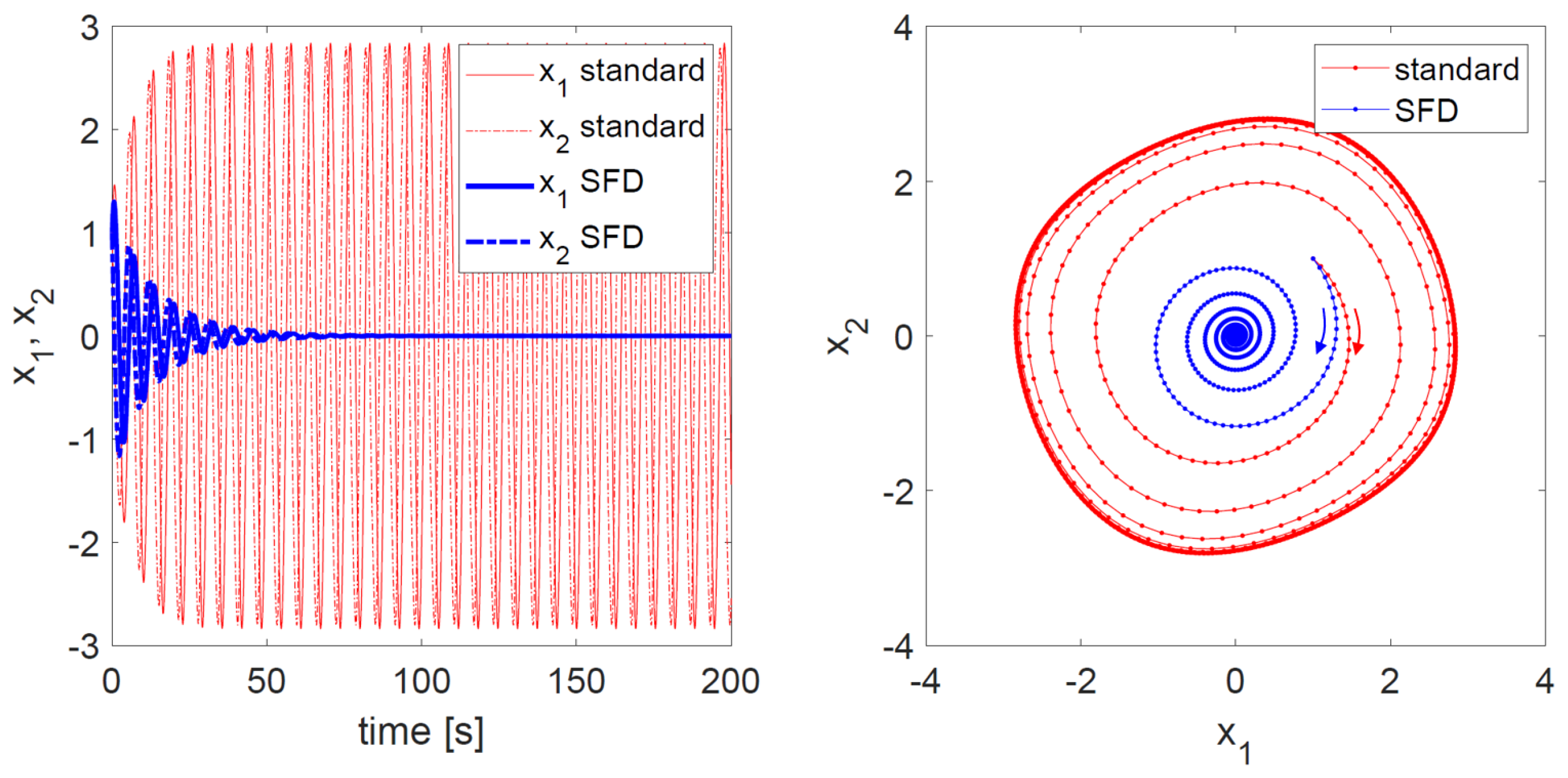
For illustrative purposes, for and an initial value of , the time-dependent solution is time-marched using the first-order forward Euler scheme with a time step size of , and a limit-cycle solution is obtained. The evolution of the solution and its phase plot are shown in Figure 8 (with the legend ’standard’). It can be seen that, although the dynamic system has a zero solution, it is an unstable one. This behavior is representative of a typical non-converging RANS solver when the underlying steady solution is numerically or physically unstable. In order to numerically obtain the unstable zero solution of the van der Pol oscillator, SFD is used to stabilize the time-marching scheme. The evolution of the solution and its phase plot are also shown in Figure 8 for comparison (with the legend ’SFD’). It can be found that SFD is able to stabilize the oscillatory solution and allow convergence to the unstable equilibrium solution . In this simple test case, the two parameters are set as and , and no further investigation is conducted to optimize the parameters for faster convergence to the equilibrium point. More discussions on selecting the parameter values appropriately are presented in the following paragraphs.
3.2.2. Sfd Stabilized Nonlinear Steady Flow Calculations
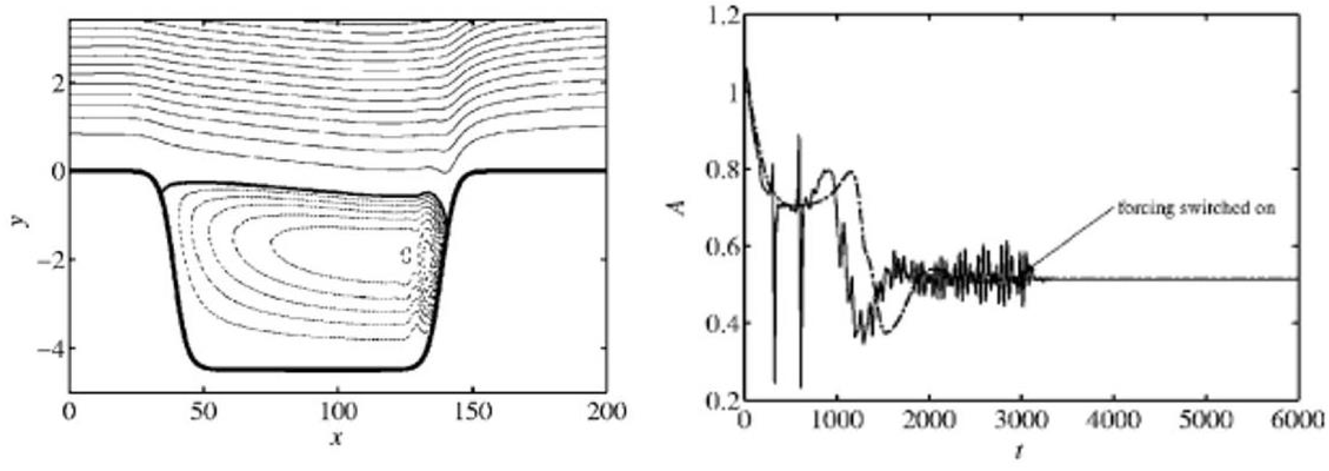
The SFD method was initially proposed and applied to the stabilization of the steady-state solutions of the Navier-Stokes equations in [13]. The two cases considered are the steady state calculations of (i) a two-dimensional flow over a long cavity, and (ii) the separation bubble induced by an external pressure distribution. The stabilized cavity flow solution is shown in Figure 9. The flow is computed for , which is chosen by gradually increasing it until the flow becomes globally unstable. In one simulation (dash-dotted line in Figure 9), SFD is turned on from the beginning, and the flow calculation converges to a steady state. In another (solid line in Figure 9), SFD is not turned on from the beginning, and the flow solution time marched using a semi-implicit second-order backward Euler/Adams-Bashforth scheme exhibits an oscillatory convergence behavior. Only when SFD was turned on at , the oscillation was suppressed, and full convergence was achieved. As expected from the theory, the steady state solutions obtained in the two simulations were identical. However, the choice of values for and was not discussed in detail in [13].
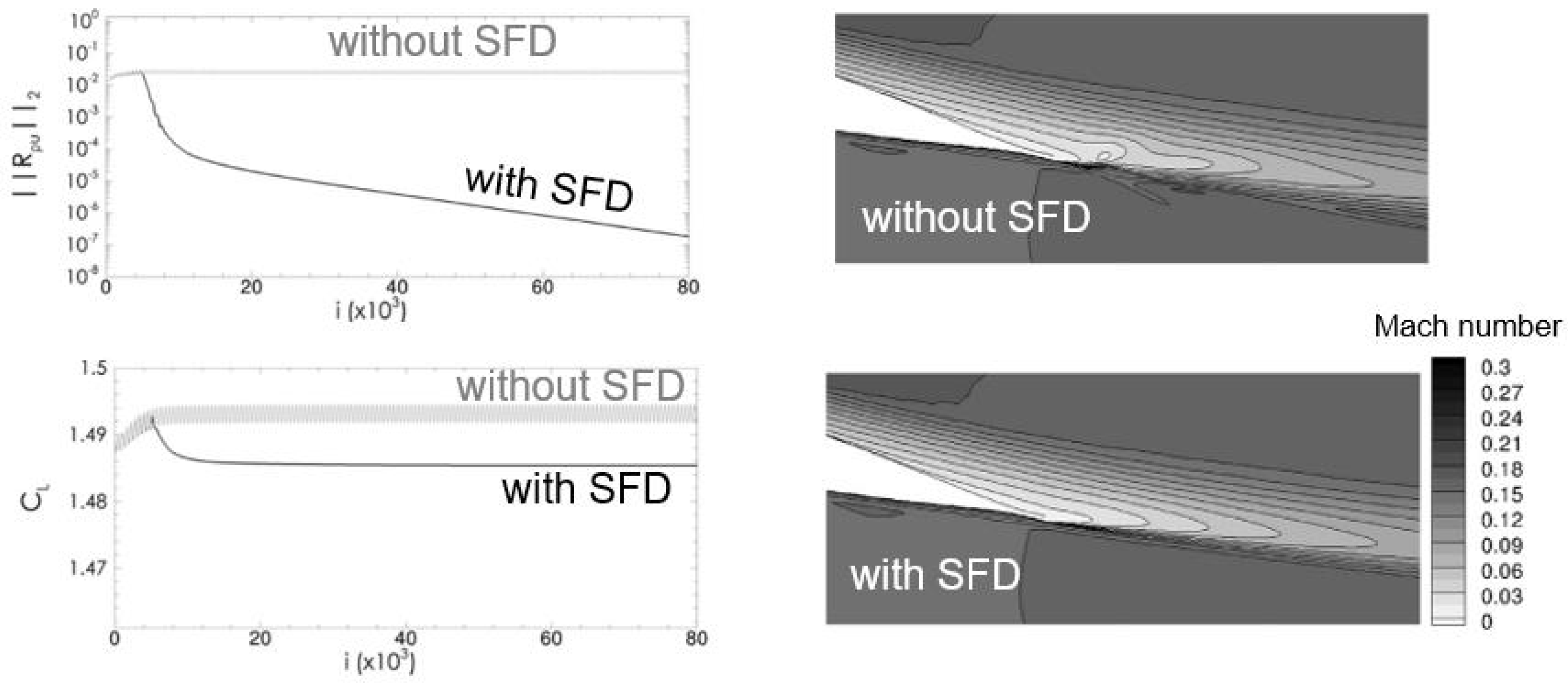
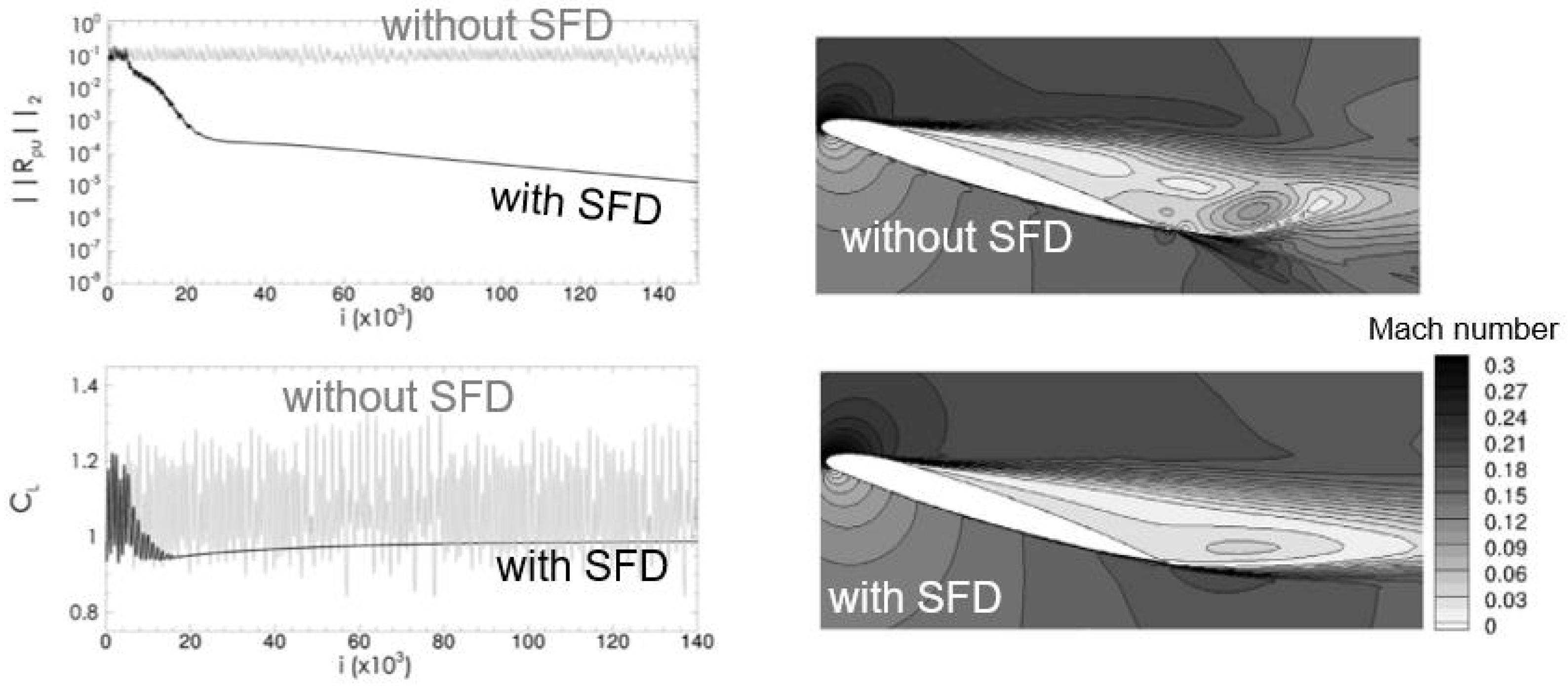
The SFD method was used to improve the convergence and robustness of the steady state solution algorithm in [27] for the turbulent flow solutions around an aerofoil at a high Reynolds number () and for angles of attack near stall. In [27], the elsA code [28] was used to time march the flow to the steady state using a local time-stepping method. For an angle of attack of , a fully converged solution can be obtained. However, for higher angles of attack ( and ), the convergence of the nonlinear flow solver stagnates and oscillates around a high residual level. With SFD, the limit-cycle oscillation convergence is avoided and full convergence of both the residual and the lift coefficient is achieved, as shown in Figure 10 and Figure 11. Although convergence at both conditions are successfully stabilized with SFD, it can be seen that the convergence of the flow for is much slower than that for .
The SFD method is used for stabilizing the unstable Navier-Stokes flow calculations performed with the Nektar++ spectral-element framework [29,30]. Although the method is reported to be convenient to implement and effective in stabilizing the flows considered, i.e., flows in a channel with a bent at and , it was also claimed that the computational cost was overwhelmingly large, despite using automatically-optimized parameters.
The only three-dimensional case for which SFD was applied to the authors’ best knowledge is reported in [31]. In order to perform global stability analysis for a jet in crossflow, SFD was first used to find the steady state Navier-Stokes solution. As the focus of that work is on the global stability analysis, no detailed description of the parameter choices and the computational cost were provided in [31].
3.2.3. Sfd Accelerated Nonlinear Flow Solvers
Similar to RPM, SFD can also be used to accelerate the calculation of nonlinear flow solutions. It was used in [32] to speed up the convergence of the Euler and RANS flow solutions over airfoils. Instead of using a global value, it is proposed in [32] to use a cell-wise varying value based on the local spectral radius. Depending on the cases, convergence acceleration of up to a factor of two in terms of CPU time is achieved. The results presented in [32] demonstrated that SFD is a promising method for accelerating the convergence to steady state for Euler and RANS solvers. However, it was also shown that the acceleration effect strongly depends on the parameter values, and although the proposed ad hoc criteria to set the value seemed to work for the test cases considered in the paper, more tests on three-dimensional RANS flow cases should be performed to evaluate the proposed criteria more comprehensively.
In [33], SFD was used to accelerate the convergence of an incompressible flow solver based on the immersed boundary method. An optimization method of the parameter pair and is developed to accelerate the convergence to the steady state, trying to minimize the spectral radius of the Jacobian matrix in the parameter space of (, ). A faster convergence rate and higher efficiency were demonstrated on the flow calculations past a cylinder and two side-by-side cylinders at , compared to the results using the original methods [13].
SFD was used for the stabilization and acceleration of steady state RANS flow calculations [34]. A novel modification to the SFD method is proposed to improve the convergence rate of the solver. The modification to the algorithm consists in the addition of a periodic reset of the low-pass time-filtered flow to the value of the base solver flow. This adds an additional parameter to the method, that is, the number of iterations between each reset. The goal is to remove the influence of previous poorly converged solver iterations. The novel modification is tested for the test cases of vortex shedding over a cylinder and transonic buffet over a supercritical airfoil. The results show an improved convergence rate with a successful stabilization of the flow solution.
3.2.4. Summary of Current Status and Suggestions for Further Development
The SFD method has been demonstrated to be an effective lightweight approach to obtain steady-state solutions for two- and three-dimensional flow calculations when unstable modes that hinder the full convergence of the nonlinear flow solver exist. Its formula is simple and elegant, requiring only minor modifications to the original algorithm, and does not alter the equilibrium point of the original system. However, finding a suitable choice of the two parameters in the augmented system, and , remains a challenge for generic problems. It was suggested in [13] that the cutoff frequency of the low-pass filter, , should be chosen according to the frequency characteristic of the unstable modes, i.e., the imaginary parts of the eigenvalues of the destabilizing modes. The imaginary part reflects the frequency of the mode and it can be relatively easily inferred from the limit-cycle oscillations of the non-converging flow solver. , on the other hand, should be set according to the growth rate of the unstable modes, i.e., the real part of the unstable eigenvalues. However, due to the nonlinear stability, the growth rate of the linearly unstable mode unfortunately does not reveal itself in the limit-cycle residual convergence history and is thus difficult to be estimated without extra work. Therefore, a somewhat ad hoc approach, simply setting , is proposed in [13]. The parameters are set according to this ad hoc rule for the simple van der Pol oscillator example shown in Figure 8. Algorithms to allow a better choice of the two parameters were discussed in [35] using an optimization approach. Specifically, the unstable eigenvalues are estimated using the dynamic mode decomposition method based on the flow solution snapshots produced during the time-marching process. This, however, inevitably incurs an extra computational cost.
Another feature of the SFD method can also be implemented into an existing nonlinear flow solver in a non-intrusive way, since the original formula of the SFD method introduced in [13] would require a modification of the solution update scheme for , coupled with an additional update procedure for . In [36], the original time–continuous coupled system is discretized using a sequential operator-splitting method and divided into two small subsystems that are solved separately using different numerical schemes. Specifically, the flow solution is first updated by one iteration using the existing solution-update scheme in the flow solver as
where the operator represents any arbitrary iterative solution algorithm of the original flow solver. The updated flow solution is then used as an input for the low-pass time filtering step
and this linear system of ordinary differential equations can be solved exactly. Due to its modified form compared to the original formula, further discussion on how to best choose the values for and is given in [36].
A downside of the SFD method is that the optimal values for the two parameters and are highly case dependent and one would need to have some knowledge of the characteristic frequency information to determine the optimal cut-off frequency in order to determine the value of . Although various techniques for providing a good estimation for the values of the two parameters exit, they all to some extent require the unstable eigenvalues of the system to be estimated and incur extra CPU time and memory overhead. The effectiveness of the SFD method for stabilizing the nonlinear solver on large-scale applications needs to be further evaluated with more tests.
3.3. Boostconv Method
Similar to SFD, the BoostConv method introduced in [14] can also be used to accelerate convergence of stable iterative solvers and stabilize non-converging steady-state iterative solvers. The method is quite recent and, therefore, has only been reported in a few papers. It is used in [37] to find the three-dimensional steady-state base flow for investigating the bifurcations formed on inserting a hemispherical roughness element in a laminar Blasius boundary layer. It is integrated as a “black-box” with a multigrid solver to accelerate convergence in solving a elliptical Poisson-like equation without additional computational cost in [38]. More recently, the BoostConv method is extended to turbulent steady flow calculations [39].
3.3.1. Theory
Consider a linear system of equation
solved with a certain iterative method as
where stands for the residual at the iteration, and B represents the effect of applying a certain iterative solution scheme to the residual vector. Multiplying both sides with A yields
The idea behind constructing the BoostConv method is to find a way to modify as , leading to a modified solution update scheme as
so that the resulting residual could be minimized. The modified solution update scheme can be transformed to the follow form by left-multiplying both side with A
which implies that the best choice for is . Computing the optimal requires solving , which is obviously not practical, since otherwise the problem would have been solved. Therefore, it is proposed in [14] that one could form a reduced-order model of by recording the solution and residual vector snapshots from the previous iterations and invert the approximate at a much lower cost. Although the analysis so far is based on a linear system, it can be extended to nonlinear iterative scheme provided that the solution variation is already sufficiently small.
3.3.2. Summary of Current Status and Suggestions for Further Development
One of the main advantage of the BoostConv method is that it can be implemented in a completely non-intrusive way. With an existing iterative linear or nonlinear solver, one only needs to provide the solution and residual vectors over the preceding iterations, and the BoostConv module can then return a modified residual to be used for solution update. Although meant to be used with a small number of solution and residual vector snapshots, it is shown for a two-dimensional RANS flow calculation over an airfoil that for a basis size of 80, equal amounts of time is being spent on the modified BoostConv method and on solving the flow [14]. Beyond a basis size of 80, the contribution of the modified BoostConv method dominates the total computational time. It is, therefore, a quite computationally expensive method when a large number of basis vectors are required, which is very similar to RPM. Although the computational cost is not a major concern when the goal is to compute a steady solution for stability analysis, the computational efficiency needs to be carefully considered when applying the method in scenarios where a large number of flow analyses in batch mode are required.
As the BoostConv method is relatively new in comparison to other stabilization methods discussed in this paper, more applications of the method in a wider range of flow calculations on more realistic geometries are needed to give a fairer account of the performance of this stabilization method.
3.4. Newton’S Method
As discussed above, both RPM and SFD methods have a limit as to what extent the nonlinear solver convergence can be stabilized, especially for the complex three-dimensional flows inevitably countered in aircraft and turbomachinery aerodynamic analysis. For edge-of-the-envelope applications, a stronger tendency for flow instability is usually associated with a large number of unstable modes and oscillations of multiple frequencies of different scales, rendering the RPM and SFD, which essentially take a divide-and-conquer approach, less effective than when applied to simpler cases. Compared with RPM and SFD, Newton’s method is a heavy-weight approach for convergence stabilization, as it in general is quite memory expensive and resolving the resulting large sparse linear system is computationally very costly. However, due to its fast convergence rate when the solution is close to the equilibrium point, it is receiving increasingly more interest, especially when deep residual convergence is desired for challenging cases. In this subsection, the Newton’s method and its applications to achieve robust and efficient convergence of both nonlinear and linear flow solvers are reviewed.
3.4.1. Theory and Mathematical Formulation
Newton’s method is an ancient root-finding algorithm for nonlinear functions. For a generic nonlinear problem of the following form
the Newton’s root-finding algorithm is simply
Despite its simplicity in form, applying it to the solution of large-scale three-dimensional RANS steady-state flow calculations remains a challenge. The first one is to obtain the Jacobian matrix A. To balance accuracy and robustness, the spatial discretization of a production-level RANS solver is usually quite complex. Therefore, differentiating the residual vector with respect to the solution vector to obtain the exact Jacobian matrix is quite tedious, if not impossible, and the memory required for storing the Jacobian is high, in comparison to the memory requirement of an explicit time-marching solver. The first and most straightforward approach to obtain the Jacobian matrix is to perturb one flow variable for each control volume at a time, and use the perturbed residual vector to obtain one column of the entire Jacobian matrix. Although the perturbation with a finite step is easy to implement and most non-intrusive, the accuracy of the resulting derivatives would depend on the chosen step size. Alternatively, one could apply the automatic differentiation technique to the residual evaluation subroutine, as for example in [40], to avoid the dependence on step size. However, this would still cost residual evaluations for a RANS solution with a one-equation turbulence model on a mesh with N control volumes. The cost can be reduced to less than 400 residual evaluations on structured grids [40] and 100–3000 for general unstructured grids [41] if a graph-coloring technique is used [42]. The coloring-accelerated approach is used in [40,41,43]. An even more efficient approach is to apply the automatic differentiation technique at the components level, instead of to the entire residual evaluation subroutine. This is the so-called hybrid approach, where one first computes the edge-based flux derivatives with respect to the left and right states, using the differentiated flux calculation subroutine, and then manually assembles the entire exact Jacobian matrix. This approach is used in [9,44]. One could also differentiate the flux subroutine by hand, which improves code efficiency compared to automatic differentiation [45]. The downside of the differentiation-by-hand approach is its low maintainability, as an adjustment of the underlying discretization algorithm might trigger the rewriting of the differentiated code, or adding a new turbulence model would require further tedious differentiation by hand. All approaches for obtaining the exact second-order accurate Jacobian matrix require storing the matrix, or at least its key ingredients on flux faces, which incurs large memory overhead for large three-dimensional cases. Jacobian-free approaches can be used to alleviate such difficulties to some extent and their various aspects have been thoroughly discussed in an excellent review paper [16]. The key idea of the Jacobian-free approaches is to obtain the matrix-vector product without explicitly forming and storing the large Jacobian matrix A. This can be done as long as the differentiated (either manual or automatic) code of residual evaluation is available. By seeding the differentiated residual subroutine with , one can easily obtain . When differentiating the residual code is not possible, one then can again resort to finite differencing and obtain the matrix-vector product via , as, e.g., in [46]. It should be noted that the Jacobian-free approach is not matrix-free. In order to perform an effective preconditioning when solving the large sparse linear system of equations , some approximate form of the exact Jacobian matrix still needs to be formed, based on which a preconditioner can be conveniently calculated [17,46].
Once the Jacobian matrix is computed, the resulting large sparse linear system of equations needs to be solved efficiently, which accounts for the majority of the computational cost of the Newton algorithm when solving large three-dimensional RANS flow problems. The techniques for solving a large sparse linear system of equations have been thoroughly discussed in [23], among which the Krylov subspace methods have become the method of choice for high-dimensional flow problems due to its robustness and efficiency. Therefore most, if not all, RANS solvers based on the Newton’s method are called Newton-Krylov solver. Among Krylov subspace solvers, GMRES solver is probably the most used one. GMRES solver finds the approximate solution to a large sparse linear system of equations
by approximating it with a linear combination of , which is a set of orthonormal vectors that spans the Krylov subspace . One first builds the m-dimensional Krylov subspace via the Arnoldi process with the modified Gram-Schmidt orthogonalization algorithm (Algorithm 1).
| Algorithm 1: Arnoldi process |
|
 |
The basis vectors and the Hessenberg matrix satisfy the following Arnoldi relationship
with and defined as
Assuming the solution to the linear system of equation x is of the following form
where is the coefficient vector for the linear combination. Then the error of the approximate solution is
Left-multiplying both sides with yields
It can be seen now that the minimization problem has be reduced from a high-dimensional problem to a low-dimensional one. It is also straightforward to verify that the solution to minimizes . Instead of solving the low-dimensional linear system of equation directly, given rotations can be used to transform the Hessenberg matrix into an upper triangular form incrementally after each Arnoldi step, which then allows the approximate solution x to be determined via y as each step.
From the GMRES algorithm, it can be seen that the memory overhead excluding that, for storing the Jacobian matrix and the right-hand-side and solution vectors, linearly scales with the number of retained vectors, m. Each step of the Arnoldi process consists of one matrix-vector multiplication and many vector-vector multiplications against previously computed Krylov vectors. When m Krylov vectors are used, the number of matrix-vector multiplications is m and the number of vector-vector multiplications is , which scales quadratically with the Krylov vector numbers, and eventually becomes the bottleneck of computational cost when m is large. Restart can be used to reduce the memory and computational cost as long as m is above a case-dependent threshold.
By construction (also suggested by its name), GMRES solver does not allow its residual to increase. However, when m is not sufficiently large, residual convergence of the GMRES solver would stagnate, and the threshold value of m is unfortunately case dependent, and not possible to be determined a priori. Therefore, in practice, m is by default set to a relatively large value as long as the storage of the computational environment permits. The reason restarting does not overcome the convergence stagnation problem is that all m Krylov vectors formed are discarded before the following cycle is executed. Algorithms to selectively recycle a small number of Krylov vectors or equivalently a subspace of dimension much smaller than m have been proposed to lower the minimal Krylov subspace dimension, and thus the Krylov vector numbers [47,48]. Some of these recycling techniques have been applied to large scale nonlinear and linearized RANS flow problems recently [4,49,50].
The system matrix for a large sparse linear system of equations arising from the linearization of the nonlinear residual for a practical flow problem is usually numerically very stiff, and even with a state-of-the-art Krylov subspace solver, convergence is rarely achieved if not used in combination with an effective preconditioner. Suppose matrix P is a good approximation of the Jacobian matrix A and easy to form and invert at the same time, then one can solve the following left and right preconditioned linear system of equations
or
to obtain x. Note that although the left and right-preconditioned systems once fully converged are identical, they are not the same when solved inexactly, which is the standard practice in Newton’s method. The subtlety of the difference between using the right or left-preconditioned has been discussed in [51]. Based on the assumption that P is a good approximation of A, it is likely that the system matrix of the preconditioned linear system of equations, , is much bettered conditioned than A itself, and thus the resulting linear system of equations is much easier to be solved, e.g., using Krylov subspace methods. Two main choices of preconditioners are incomplete LU (ILU) and multigrid. A general ILU factorization process computes a sparse lower triangular matrix L and an upper triangular matrix U so that the residual matrix satisfies some constraint. Among various variants of ILU, the most popular version is probably incomplete LU factorization technique with no fill-in, denoted by ILU(0), taking the zero pattern of the factorization matrices to be precisely that of A. When the accuracy of the ILU(0) incomplete factorization may be insufficient to yield an adequate rate of convergence for some cases, ILU(p) can be used, with a higher level of fill in the resulting L and U matrices. However, since a higher level of fills naturally increases the memory overhead and also adds to the number of floating-point operations during the application of the preconditioner, the improvement of the preconditioning effect, reflected as the reduced iteration to convergence for the preconditioned Krylov solver, the increased memory and computational cost of forming and applying the preconditioner need to be considered in order to find an optimal level of fills in practice.
The ordering of the unknowns can significantly affect the performance of ILU preconditioning, as was discussed thoroughly in [52] and further elaborated in [52]. It was suggested that reverse Cuthill–McKee (RCM) ordering [53] to be the most effective for the multi-block structured solvers considered in their work. However, in contrast, it was found in [54] for an LU-SGS solver that reordering only marginally affects the computational efficiency in the unstructured solver considered. However, as this solely affects the computational efficiency and theoretically has no effect on the solver stability, the issue of not further discussed here.
A final remark on the ILU preconditioners is that, although it is most straightforward to calculate the ILU factorization matrices based on the system Jacobian matrix A, in practice, it has been observed independently by different researchers that it is more effective to base the preconditioner on the Jacobian using a lower-order discretization. For example, for various independently developed second-order accurate RANS solvers, it has been reported that, although A is exactly based on the second-order spatial discretization, the preconditioner is computed using the approximate Jacobian based on the first-order spatial discretization [4,41,43]. Basing the ILU preconditioner on a lower-order residual discretization has also been shown to be useful for higher-order RANS solvers [55]. A rigorous proof for this is not available in the open literature. A plausible explanation is that the loss in accuracy due to the lower-order approximate Jacobian is compensated by a much more accurate resulting ILU factorization due to the reduced bandwidth and improved condition number.
A second major class of preconditioners is multigrid [56]. Multigrid has been traditionally proposed for elliptic partial differential equations. The central idea is to accelerate the convergence to solution by off-loading the slow-converging low-frequency error modes on the fine grid to coarser ones, where the low-frequency error modes become fast-converging high-frequency ones. The most appealing feature is that multigrid theoretically produces mesh-independent convergence rate, that is, the iteration to convergence does not depend on the mesh size. However, such mesh-independent convergence rate has rarely, if ever, been observed for practical three-dimensional turbulent flow problems, although significant convergence acceleration indeed could be achieved [57]. Furthermore, applying it to unstructured meshes introduces other practical issues such as efficient and robust unstructured mesh coarsening algorithms [58]. Multigrid methods are traditionally geometric ones where one first needs to produce a sequence of gradually coarsened grids. It has then been generalized as algebraic multigrid (AMG) [59,60], which does not require the coarse grids to be available at the first place, but instead, extends in a purely algebraic manner the fundamental principles just described to general sparse linear systems. AMG has also been used in some of the production-level RANS solvers with some success [61,62]. However, systematic comparison of the ILU versus the multigrid preconditioner has rarely been reported, possibly because perfecting the implementation of each algorithm in a state-of-the-art is already a rather extensive effort. Another possible reason is that the performance of multigrid preconditioner, especially geometric multigrid, is highly dependent on the underlying residual discretization scheme, meshing strategy, coarsening algorithm, etc., and therefore it is difficult to present a comparison that can be generalized to a different solver. Nevertheless, due to the essential role of the preconditioner on the overall computational efficiency of the underlying CFD solver, more research into the preconditioning technique is urgently needed.
With the Jacobian matrix computed, and an effective preconditioner constructed, the final difficulty of achieving a fast, quadratic residual convergence promised by the theory, is the globalization, or solver steering techniques. It is well known that the Newton’s root-finding method relies on a good initial guess to stably converge, and for practical applications, converging the flow towards the basin of attraction, not only stably but also efficiently, is a challenge. The key to the solution steering technique is to find a suitable relaxation factor when updating the flow solution after an approximate linear solution is found in Equation (60) as follows
Some of the earliest attempts to globalize Newton’s method include [63,64], in which the nonlinear system of equations due to the discretization of flow equations are iteratively solved using the Newton’s method, and the inner linear system of equations are solved using GMRES, thus the so-called Newton-GMRES algorithm, which is nothing but the more commonly used terminology of Newton-Krylov with GMRES being the Krylov subspace methods. It was in these work that the backtracking technique was used to stabilize the Newton nonlinear iteration. Backtracking essentially means applying an appropriate relaxation factor to optimize the nonlinear residual drop each time a linear solution is computed. It was also in these early work that the term inexact Newton method was coined, where ’inexact’ means the linear system was only solved approximately, as fully solving it, would in turn results in an overall slower nonlinear solver convergence, in terms of the CPU time. Furthermore, it was also found that sometimes oversolving the linear system to obtain a more accurate would even cause the nonlinear residual convergence to stall, due to a failure of the backtracking [65,66]. This is explained differently, and probably more insightfully in [67], as the backtracking technique based on the linear search methods stagnates due to encountering local minima of during the solution evolution. Pseudo-transient continuation (PTC), among many other continuation methods [16], is an effective way of avoiding being trapped in local minima of . This is inspired by the fact that the underlying physical system, which in our case is the flow field, would never stagnate as observed in Newton’s method. This intrinsic physical property is retained in the numerical method by including the time derivative in the governing equation, even when a steady-state solution is sought. With this in mind, instead of solving , one solves the following nonlinear system of equations using Newton’s method
As only steady-state solutions are concerned, time accuracy is not necessary. Therefore, a simplistic first-order backward Euler scheme can be used to discretize the time derivative, and the resulting discretized nonlinear governing equations are
Note that the time step can also vary on each control volume, again as time accuracy is not necessary. In practice, the time step for each control volume is the maximal time step estimated from the spectral radius of the local flux Jacobian matrices multiplied by a global Courant number , as
The Courant number can be viewed as the continuation parameter, which evolves from an initially very small number for solver robustness during the initial stage of computation to a large value towards full residual convergence, when the standard Newton scheme can be recovered and quadratic convergence can be achieved. The key to the success of such PTC technique is then to design an appropriate rule for the Courant number to evolve as fast as possible but still not destabilize the nonlinear iteration.
One early practical application of the PTC technique was [68], in which the successive evolution–relaxation (SER) strategy for evolving the Courant number automatically was proposed. The SER strategy allows the time step to grow in inverse proportion to residual norm progress:
Although the SER strategy has been used in many early work on Newton-Krylov solvers, our experience with the method on practical three-dimensional flow calculations has been that it is not sufficiently robust, especially for cases with strong initial flow transient where flow reversal appears, or turbulent flow cases where the turbulence variable field rapidly grows in the initial convergence stage. In those scenarios, the nonlinear residual can grow up to three orders of magnitude during the first few nonlinear iterations, and once the Courant number reaches a much lower value, it in turn renders the flow evolution very slow, causing the overall nonlinear iteration to nearly stagnate. This difficulty of course can be alleviated substantially if a more suitable scheme, for example, the explicit Runge-Kutta scheme, is used during the initial convergence stage and one only switches to Newton’s method with PTC based on SER when the residual starts to monotonically drop. However, such switch is usually a result of trial and error, and thus the moment to perform such a switch is most likely not optimal. Examples of such predetermined switching between solution phases are shown in [55] where the Courant number over the first few iterations are prescribed. Although effect for the cases discussed in [55], it is likely that for a different set of cases, the predefined Courant number evolution schemes are sub-optimal. Secondly, having to perform such a switch makes the algorithm less automatic and elegant, thus causing additional burden on the application engineers who naturally prefer to turn as few knobs as possible in practice. The authors are thus not in favor of the SER strategy. An alternative is to adapt the value of based on the line search/backtracking result. If the line search returns a favorable step near unity, then it implies the Newton iteration is progressing well, and therefore it is safe to ramp up the Courant number by a factor; on the contrary, if the line search returns a step that is deemed too small, then it implies the nonlinear residual is encountering a local minimum and it is better to reduce the Courant number by a factor in the subsequent step to avoid residual convergence stagnation. Although the particular values of the growth and reduction factors are different among different researchers that adopt this strategy, they all in principle follow this approach [3,69,70].
Even with all the tricks introduced above, it is still possible that the PTC Newton algorithm might break down due to a diminishing Courant number. A further algorithmic improvement was proposed in [70], which combines the robustness of explicit local time stepping with lower per-iteration cost at the initial convergence phase and the fast convergence of Newton steps towards full convergence. Based on the experiences that explicit and point-implicit solvers are surprisingly stable with a Courant number , while when the PTC Newton scheme encounters convergence stagnation, it is essentially evolving the solution with a Courant number . It is speculated that the convergence stagnation constantly encountered is due to the non-smooth residual distribution of the explicit or point-implicit iteration when the Courant number is small, and thus the nonlinear solver is difficult to recover from it. To circumvent this problem, it was proposed in [70] that the following time-marching scheme
which for reduces to
and for reduces to the standard Newton scheme. The advantage of this is that when , instead of resulting in a stagnating residual convergence due to a diminishing Courant number, the nonlinear iteration scheme would still effectively damp the residual as in conventional nonlinear time-marching solvers, for example, using a block-Jacobi scheme or even an explicit forward-Euler scheme with . Furthermore, adding the multistage Runge-Kutta flavor into the operator D helps smoothing the residual field which in turns facilitates the PTC Newton iteration to progress more successfully. The resulting PTC Newton scheme incorporating the residual smoothing strategy was shown to be significantly more robust than the one without it for three-dimensional turbulent transonic flow calculations [70].
A similar strategy was proposed in [71], which focuses on the robustness of a Newton-Krylov RANS solver at the startup phase. Instead of using the exact Jacobian matrix augmented with a pseudo time stepping to augment the diagonal blocks, as done in most PTC Newton solvers, it is proposed that an approximate Jacobian should be used at the startup phase (thus an approximate Newton-Krylov (ANK) scheme), and one only switches to NK, which features an exact Jacobian matrix and a pseudo time step of infinity once the nonlinear residual has dropped by five orders of magnitude. This is rationalized by three reasons. First, when the pseudo time step size is small at the startup phase with a PTC NK approach, the advantage of using an exact Jacobian is not fully used, and the overall effect of the compromised accuracy due to replacing the exact Jacobian with an approximate one is marginal. Second, using the approximate Jacobian offers a large degree of freedom to apply various levels of approximation, for which the residual calculation stencil can be reduced significantly, resulting in a much more efficient Jacobian calculation. Finally, even with the exact Jacobian, as mentioned above, the preconditioner is usually still based on an approximate Jacobian, which in the proposed ANK startup strategy in [71] is computed and stored anyway and can be made use of directly. The numerical experiment results in [71] on large-scale RANS CFD calculations show that the proposed ANK startup strategy offers some advantage over the standard PTC NK algorithm. However, some tests with the aggressively approximated Jacobian are not convergent (e.g., ‘-coupled’ in Figure 3 in [71]), which hints that an overly crude approximation might instead compromise the solver stability, and therefore one should be cautious to what extent such approximation should be performed. From this perspective, it could be postulated that using ANK for the startup phase, despite its advantage in computational efficiency, could potentially deteriorate solver robustness.
With all the implementation aspects considered above, it is not surprising that, only until recently, Newton’s method has been used to solve three-dimensional RANS equations on cases with industrial relevance [70,72,73], although it has been used to solve three-dimensional flow problems three decades ago [15,68]. A majority of the literature on using the Newton’s method to solve RANS flow problems focused on aircraft applications, presumably because the flow is relatively benign and mostly attached for such applications (except those focusing on edge-of-the-envelope conditions such as shock-buffet and high-lift configurations). It was recently extended to the turbomachinery applications for both nonlinear flow and linear adjoint analyses [40]. Although Newton-Krylov algorithms are mainly used for convergence acceleration or stabilization of the nonlinear steady flow problems, they are to a large extent also driven by the need to find a fully converged solution on which linear analyses, such as stability or adjoint analyses, can be performed [43,73].
3.4.2. Stabilization and Acceleration of Nonlinear and Linear Solutions
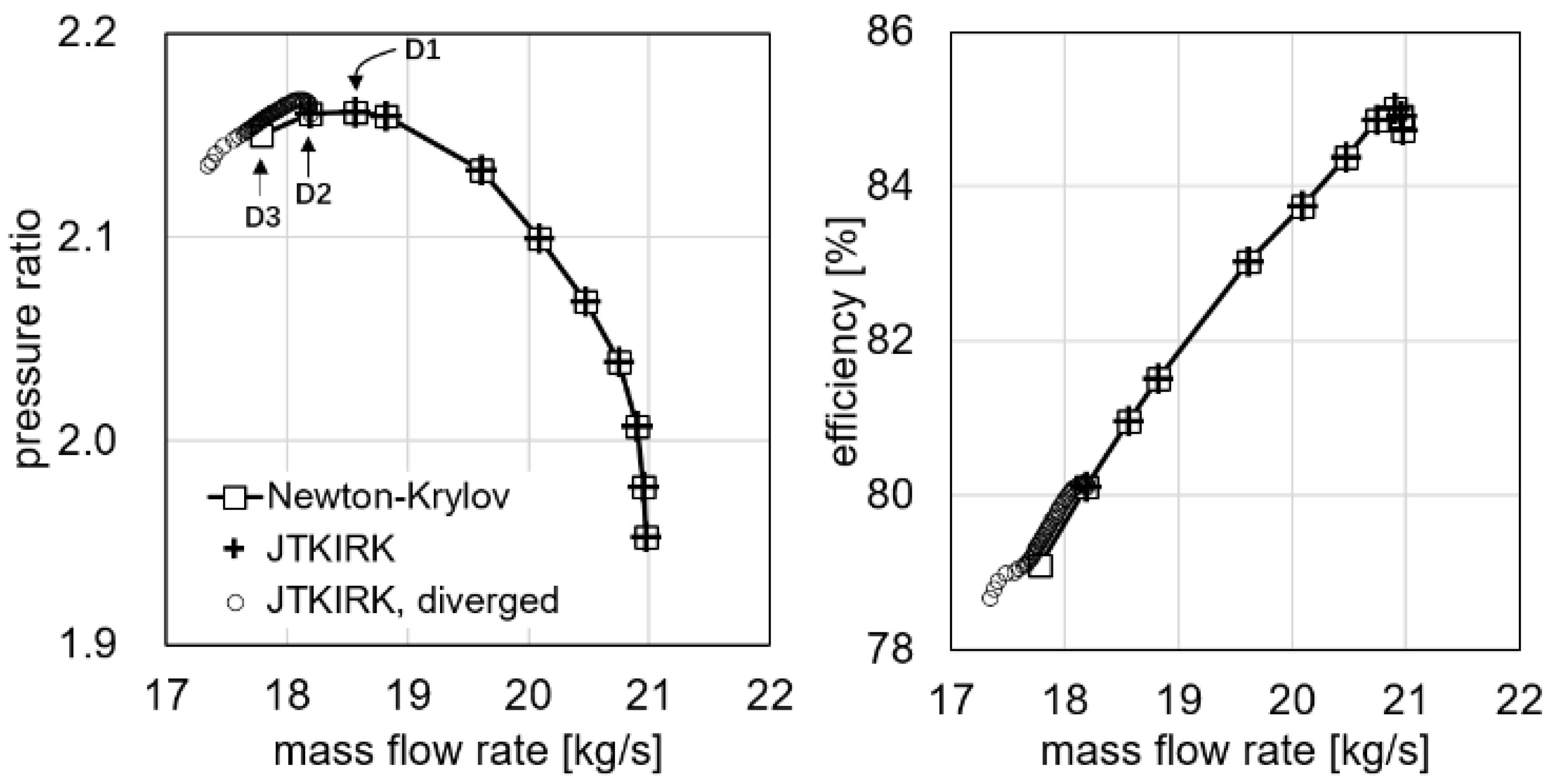
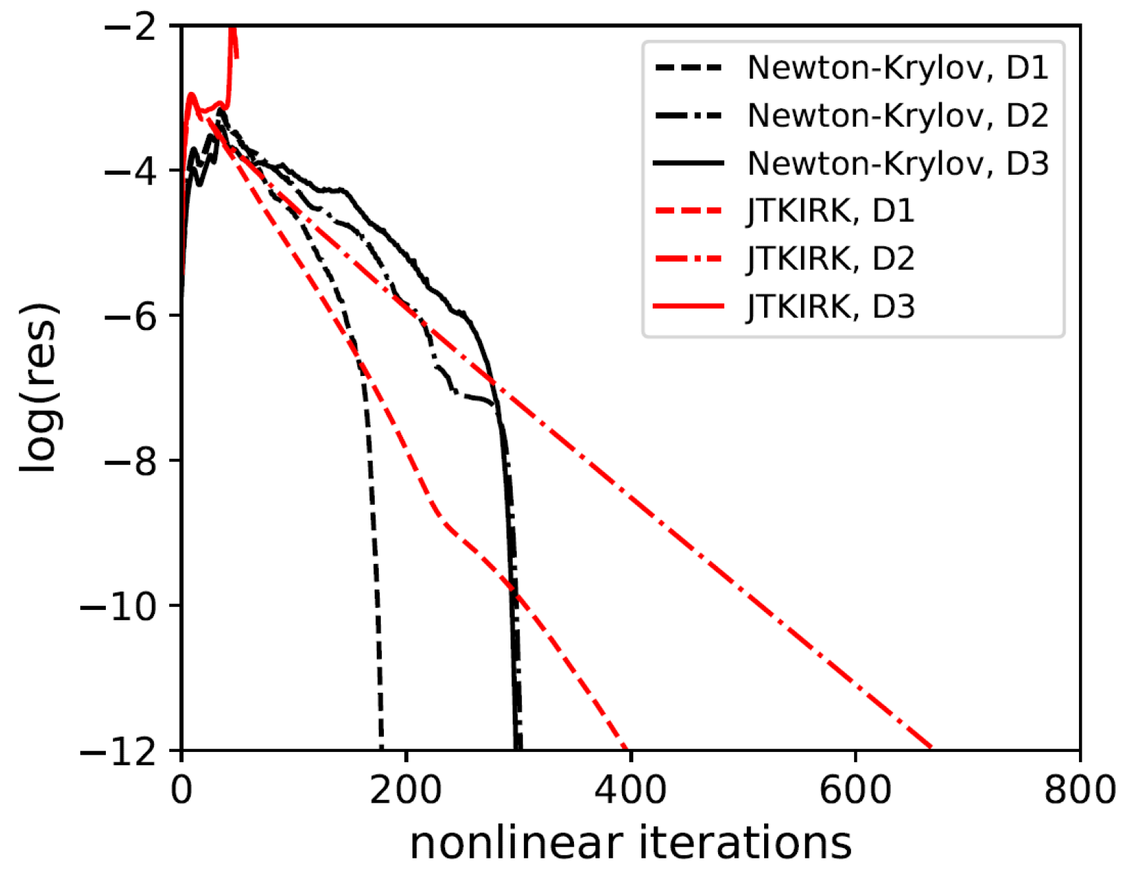
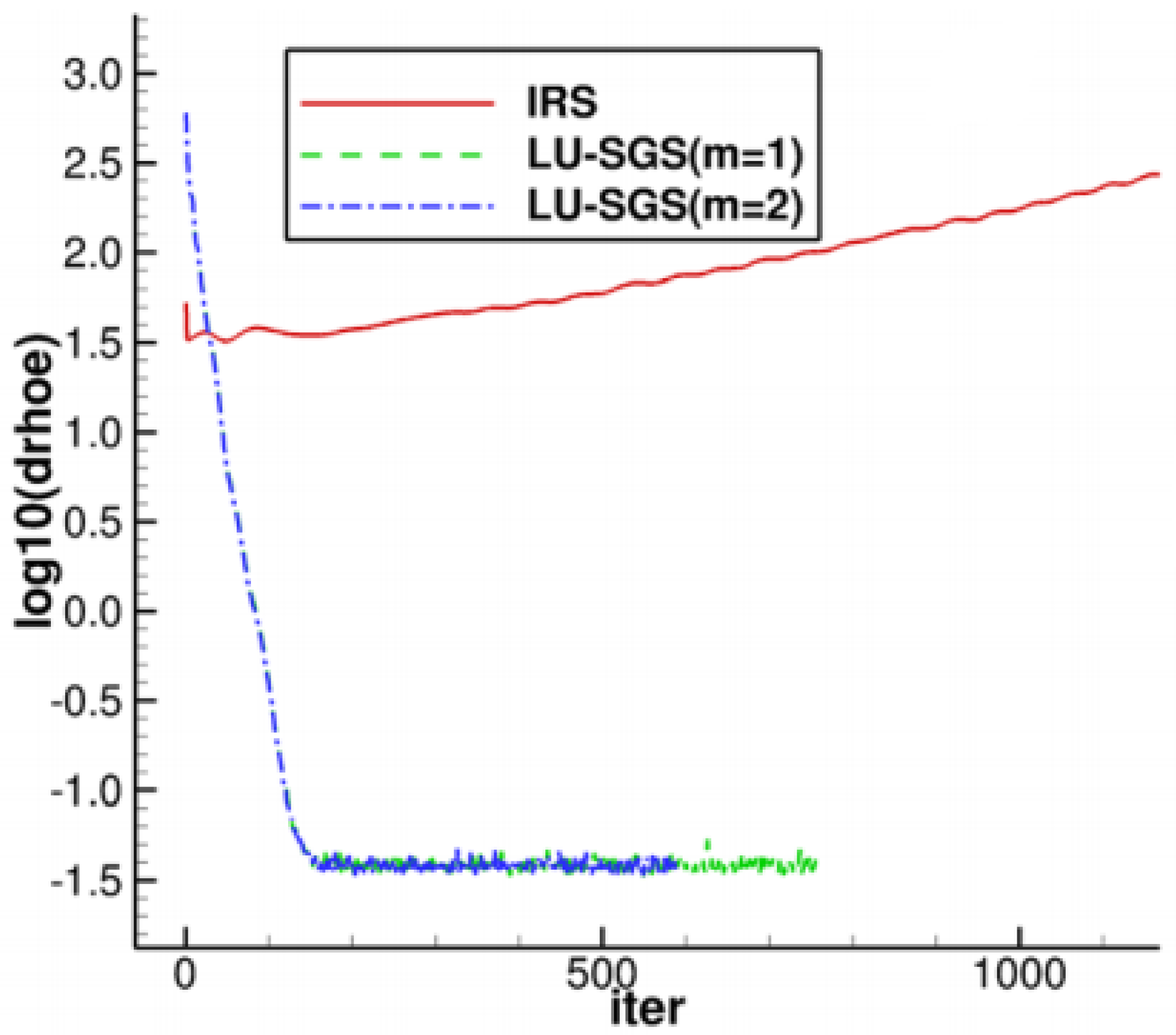
In [43], the NK method is realized for an adjoint solver for turbomachinery aerodynamic optimization. The speedline for a compressor at a constant rotational speed is computed using the NK method. Due to the robustness of the globalized Newton iteration, the speedline can be computed in a fully automated fashion. Compared with a typical implicit scheme Jacobian-trained Krylov implicit Runge-Kutta (JTKIRK) [11], which has already been shown to be quite stable, the NK algorithm can further extend the numerically stable operating regime of the compressor, as shown in Figure 12. In Figure 12, D1 is an operating condition for which both solvers can fully converge. D2 is the last condition the JTKIRK solver can converge, while D3 is the last point the NK solver can converge. The evolution of the flow solution (marked as a trajectory of circles) computed using JTKIRK starting from the converged solution at condition D2 is also shown, which eventually evolved to a non-physical state, which caused the solver to diverge. The residual convergence history of the flow solver, using both algorithms for conditions D1, D2, and D3, are shown in Figure 13.
Regarding finding linear solutions, for either time-linearized, tangent-linear, or adjoint problems, instead of using time-marching methods, during which one risks experiencing a non-converging FPI, one can directly solve the large sparse linear system of equations once using a strong linear solver. When the linear solver used is a Krylov subspace solver, the resulting solution scheme is essentially the NK approach applied to linearized problems. In [74], GMRES is used to stabilize an unstable FPI-based time-linearized analysis problem, which has previously been stabilized using RPM in [5]. A pitfall of directly solving the linearized problem using Krylov methods is that the strong linear solver will converge, as long as a sufficient number of Krylov vectors are used, regardless of the convergence of the nonlinear flow problem. Computing the linear solution for a not fully converged base flow, one risks introducing an error in the resulting linear solution. This issue was discussed thoroughly in [75] regarding the adjoint sensitivity computed using either a limit-cycle or fully converged base flow. Although the error that can be potentially introduced is highly case-dependent, one should be aware of such risk. This, in turn, demonstrates the importance of obtaining a fully-converged nonlinear flow solution using a strong implicit scheme, such as NK.
3.4.3. Summary of Current Status and Suggestions for Future Development
Despite its various advantages, the Newton-Krylov method remains a heavy-weight approach with a significant memory overhead, even with the Jacobian-free approach. It is not always advantageous over competing methods based on time-marching in terms of CPU time efficiency and memory overhead when only the nonlinear flow solutions are concerned. That to some extent explains why certain users still use time-marching implicit scheme for nonlinear flow calculation, as well as Newton-Krylov (with only one Newton step) for linearized analysis. In addition, developing an Newton-Krylov solver imposes some extra constraints on the spatial discretization, as the nonlinear residual function ideally should be differentiable, which otherwise is not required. Obtaining the exact Jacobian matrix is tedious and requires nearly perfect attention to the details of the underlying spatial discretization. However, this can be alleviated by using a Jacobian-free approach. Finally, although the NK approach promises fast asymptotic convergence, evolving the intermediate solution to near the final equilibrium point still heavily relies on a very robust solution-steering technique and consensus does not seem to have been reached as for which strategy is optimal. However, if the main driver of obtaining a deeply converged nonlinear flow solution is to perform linear analyses, then the large memory overhead, high CPU time cost, and the difficulties of developing an NK solver sometimes could be justified. Probably, this is due to this reason that the Newton-Krylov method is more often discussed in the RANS CFD-based global stability analysis or adjoint shape optimization community than elsewhere.
For further development, a robust startup strategy probably is worth the most attention, and indeed it is a heated topic among recent papers on Newton’s method [70,71]. Besides, the large sparse linear solver used in most work from the RANS CFD community has almost unanimously been ILU preconditioned GMRES since the day Newton’s method is introduced. Over the past few decades, significant progress has been made in the field of computational methods regarding the Krylov subspace methods and preconditioning techniques. For example, directing adopting an advanced Krylov solver leads to a significant speedup of linear analyses [4,50]. Among the improved Krylov methods, the ones using deflation techniques [48,76] are particular worth-noting, as they can directly substitute GMRES with a net performance gain. Krylov methods inevitably scale poorly on massively parallel machines due to the frequent global communications in the Arnoldi progress, and this has been recently addressed with pipelining [77]. Regarding preconditioning, since in most work, ILU is used for each parallel partition in an additive Schwarz fashion, which is intrinsically not scalable in terms of nonlinear iteration counts due to the decoupling at partition boundaries using a global ILU on the other hand would incur large parallel communication cost. To circumvent this problem, a communication-avoiding ILU algorithm has recently been proposed [78], and its effectiveness in accelerating the preconditioned Krylov solvers is worth investigating.
3.5. Implicit Methods
Although the Newton-Krylov method is superior in terms of its robustness and fast convergence towards the equilibrium point, its high memory overhead, the requirement of a reliable solver steering strategy and the programming complexity still pose a challenge for its wide deployment. A good trade-off between the NK method and the potentially unstable explicit or weakly implicit time-marching method is to use an implicit time-marching scheme that is just strong enough. Note that, although the Newton-Krylov algorithm can be reviewed as one of the implicit methods, in this section, the terminology ‘implicit methods’ specifically refers to those excluding the Newton-Krylov ones. Similar to Newton-Krylov, there exists an even larger body of the literature on the topic of implicit schemes for RANS solvers, and it is not the intent of this review paper to exhaust them. In this section, we only outline some of the main algorithmic aspects of implicit methods.
Implicit schemes for compressible RANS equations in general can be expressed as
where the left-hand-right matrix P is some approximation to the exact Jacobian. Depending on the specific approximation method, the resulting approximation matrix can either be a large sparse block matrix or a block diagonal matrix by neglecting the contribution of the residual contribution from neighbouring control volumes. For the former, a large sparse linear system of equations have to be solved. Traditionally, this has been solved using approximate factorization (AF), and more recently it is also common to be solved using Krylov methods. For the latter, one could directly invert each block of the system matrix at a rather low cost.
One of the most widely used approximate factorization method is lower-upper symmetric Gauss Seidel (LU-SGS) [79]. The sparse matrix P is formally decomposed as
where L, D, and U are lower triangular, diagonal, and upper triangular matrices, respectively. The symmetric Gauss-Seidel algorithm approximately solve the linear system of equation , assuming an initial value of via the following two-step process
Combining the two steps yields
Assuming that x is initialized with zero, the application of LU-SGS yields
As LU-SGS essentially factorizes P as , albeit approximately, it can also be viewed as an AF method. To quantify the error of such an approximation, note that the exact solution to the linear system satisfies
Therefore the introduced error equals , which when the matrix P exhibits diagonal dominance, would be relatively small. Note, also, that LU-SGS is mathematically identical to applying symmetric Gauss-Seidel (SGS) one time with a zero initial value for x. The advantage of the LU-SGS method is that it can be implemented in a matrix-free manner, as the entries of D, L, and U can be computed on the fly when performing forward and backward substitutions. Additionally, unlike NK or ANK methods, no excessive iterations are needed, and nor is the memory and computational cost incurred by using a preconditioner. The cost of performing one LU-SGS iteration is close to performing one sparse matrix-vector multiplication. Therefore, the LU-SGS method has been used extensively for RANS CFD calculations. Although LU-SGS can be used as in isolation to inexactly solve the sparse linear system of equation in the ANK framework, it is more frequently used as a smoother for multigrid in full approximation scheme (FAS), such as in [79]. A simpler approach is to use a single Jacobi sweep rather than Gauss-Seidel, which is reported to be effective as a smoother for a multigrid solution of the RANS equations on stretched grids [80]. Either the LU-SGS or Jacobi iterative smoother has been shown to be a memory-efficient approach, which can directly replace the more classical Runge–Kutta smoother in a multigrid algorithm.
Although LU-SGS is in general very robust and permits a large Courant number and thus fast convergence, it is analytically shown for an Euler case that neither the exact nor the approximate Jacobian due to a linearization of the nonlinear residual is diagonally dominant. Therefore, a modification to the Jacobian matrix is proposed in [54] to guarantee diagonal dominance and enhance iteration robustness. However, the augmented robustness is accompanied by a slower convergence, which presumably can be attributed to the amplified inconsistency between the left- and right-hand-side terms of the sparse linear system of equations solved. Alternatively, one could augment the diagonal with a pseudo time derivative, without altering the approximate Jacobian itself. In this case, a globalization strategy is then required to vary the pseudo time step to balance robustness and efficiency.
In addition to the investigation of convergence acceleration effect of LU-SGS, various aspects of making the iterative scheme stable are also studied in detail in [54]. It is emphasized that, in order to stabilize the convergence, it is critical that all fluxes, including both the convective and the viscous fluxes, as well as the source terms, especially those associated with the turbulence model, need to be taken into consideration. Inclusion of these key ingredients significantly enhances the solver robustness, even when the Jacobian is an approximate one.
The approximate Newton method has also been investigated as another way to formulate the implicit schemes, with some early work dating back to nearly three decades ago [15]. The approximate Jacobian is analytically computed in these early work, while nowadays it is often computed with the aid of automatic differentiation or finite differencing. The change in trend is largely due to the increase in the complexity of CFD codes nowadays, which makes the analytic or manual differentiation less attractive. The implicit scheme proposed in [15], with ILU or SGS as a preconditioner for the Krylov solver, marks probably the earliest attempt of the later-called ANK algorithm. An interesting comparison can be made between the ANK in [15,71], where one could clearly see the increase in the complexity of the cases studied and consequently the increased sophistication of the numerical schemes, although the key ingredients remain unchanged over the past thirty years.
Another worth-mentioning development is the combination of ANK and multigrid. As first discussed in [15], the ILU preconditioned Krylov solver is used as a linear solver at each nonlinear iteration without multigrid. This is not without a reason. Although much weaker iterative schemes such as Runge-Kutta converges much slower than Krylov methods, they in general exhibit a very good high-frequency damping property, compared with, e.g., forward Euler scheme, and this feature renders RK good and smoother for multigrid. In-depth analysis of the damping property of the implicit RK scheme with SGS as the smoother has been performed in [81,82,83], motivated by the desire to understand its use in combination with multigrid. Inspired by this, methods to incorporating Krylov methods into a multigrid solver was explored in [11]. By wrapping the GMRES iteration inside each step of an m-step RK scheme, one achieves both drastic low-frequency damping of a forward-Euler method, and the high-frequency damping property of RK. The modified RK is thus the so-called implicit RK (IRK), which is then used as a smoother for multigrid. The resulting implicit scheme, called Jacobian–trained Krylov–implicit–Runge–Kutta (JT-KIRK) was compared with SGS, and shows some improvement in CPU time. A similar algorithm was proposed in [24], but with the agglomeration multigrid. Instead of using GMRES to solve the inner linear system of equations, a line-implicit SGS method is used [24], where one needs to detect ’linelet’ from the surface nodes into the interior domain and orders the nodes such that SGS first sweeps over the nodes along the linelets to capture the strong coupling effect of the shear flow in the boundary layer. However, the line implicit method significantly increases the burden of the preprocessing step, and therefore not surprisingly is only adopted by very few research groups.
3.5.1. Stabilization of Nonlinear Steady and Adjoint Solvers
An example of demonstrating the stabilization effect of a strong implicit scheme on both the nonlinear and adjoint flow calculations is discussed in [11]. The strong implicit scheme uses an approximate Jacobian based on the first-order spatial discretization to control the time stepping, and the approximate Newton scheme is further wrapped inside a Runge-Kutta time stepper. The resulting implicit Runge-Kutta scheme is used as a smoother for the geometric multigrid to accelerate and stabilize the residual convergence of a nonlinear flow solver. As for the discrete adjoint equation systems, the approximate Jacobian is transposed to precondition the adjoint system, whose system matrix is a transpose of that of the nonlinear flow system. By doing this, the overall operators for time-marching both the nonlinear flow and the adjoint solutions have the same spectral radius and the adjoint solver faithfully inherits the linear stability of the nonlinear flow solver. By replacing the block-Jacobi smoother in an existing production-level flow/adjoint solver with the proposed first-order Jacobian, both the flow and adjoint calculations were stabilized. In Figure 14, the residual convergence history of the nonlinear flow and linear adjoint solvers on a high-pressure turbine stage is shown. For this case, small oscillations exist in the tip leakage flow of the turbine rotor, which prevent the original nonlinear flow solver from fully converging, and instead, it converges into a limit cycle. As a result, the adjoint analysis with the semi-converged flow solution diverges exponentially. Using the proposed implicit scheme based on the first-order approximate Jacobian allows both the nonlinear and adjoint solvers to fully converge. Using a strong implicit solution scheme, therefore, is shown to significantly enhance the robustness of adjoint analyses for cases with industrial relevance at a cost that is substantially lower than a Newton solver.
3.5.2. Stabilization and Acceleration of Frequency Domain Solvers
A nonlinear frequency domain solution using the time domain harmonic balance method is much more difficult to be obtained in an implicit way than its steady counterpart. This is attributed to the coupling of solutions at different time instants, making the size of a solution problem grow proportionally with the number of time instants. To reduce programming complexity and make use of existing implicit steady solvers, the implicit time integration of the time spectral source term of a time domain harmonic balance equation system is often decoupled from that of the remaining terms.
In [84], the implicit time integration is achieved by using the LU-SGS method for the spatial terms and the block Jacobian iteration for the time spectral source term. Compared with the usual implicit residual smoother (IRS) with an explicit Runge-Kutta scheme, the LU-SGS smoother greatly enhances the stability of the solution process. Figure 15 shows the stabilization effect of the proposed LU-SGS residual smoother compared to the original IRS approach that was non-converging, for a turbomachinery blade flutter analysis. In [85], an approximate factorization is used to decouple the implicit time integration of the time spectral source terms from the remaining terms. The advantage of this treatment is that different pseudo-time steps can be used for the time spectral source terms and the remaining terms, resulting in enhanced solution stability.
Implicit time-marching methods have also been used to accelerate time-spectral solvers. In [86], a block-implicit algorithm is proposed to accelerate the residual convergence. A much stronger implicit algorithm using GMRES is proposed in [87] to solve time-spectral aerodynamic and aeroelastic problems on unstructured meshes. The use of GMRES as the linear solver is reported to make time-spectral methods more robust, thus allowing them to be applied to problems with a broad range of harmonic content, and vastly improves the efficiency of time-spectral methods.
4. Conclusions
In this paper, five stabilization techniques, namely, (i) recursive projection method (RPM), (ii) selective frequency damping (SFD) method, (iii) BoostConv method, (iv) Newton’s method, and (v) implicit methods, are reviewed. The underlying causes for the lacking of convergence of nonlinear and linear solvers, including time-linearized and adjoint solvers, are first analyzed and attributed to the existence of unstable modes in the underlying Jacobian or preconditioned Jacobian due to unstable fixed-point iterative (FPI) schemes. The various stabilization methods are discussed in depth, respectively, including their mathematical formulations and algorithms, examples of applications, and limitations and aspects for further improvement.
The RPM method selects modes corresponding to unstable eigenvalues of the underlying FPIs and applies the Newton’s method to update the small number of unstable modes. It can be implemented in a non-intrusive manner and has been shown to be able to stabilize time-linearized and adjoint solvers for aeronautical applications. For stable cases, it can also be used to accelerate convergence. Although it can theoretically stabilize any unstable FPIs, the cost associated with storing sufficient solution snapshots to resolve the unstable modes as well as inverting the low-dimensional Jacobian matrix can be substantial for large scale cases with greater flow and geometry complexity.
Similar to RPM, the SFD method damps the unstable modes that exhibit characteristic frequencies above the cut-off threshold via low-pass temporal-filtering technique. SFD does not explicitly resolve the unstable modes as RPM, and instead it uses an additional simple differential equation to realize the low-pass time-filtering effect. The resulting algorithm requires minimal modification to existing iterative schemes and can even be made non-intrusively. Different from RPM, SFD has been used to stabilize and accelerate nonlinear flow solvers, but, theoretically, it is also applicable to linear solvers as long as the diverging modes exhibit some frequency characteristics, e.g., when the eigenvalue outliers exist in complex conjugate pairs. The main inconvenience when applying SFD is that two parameters, namely, and , need to be specified. Although some guiding principles and optimization-based approaches can help determine their appropriate values, choosing an appropriate value still requires some computational efforts. Furthermore, since the low-pass temporal filtering alters the error damping property of the FPI, SFD-stabilized iterations are in general reported to lead to slower convergence, albeit stable. Since SFD has traditionally been used to obtain fully-converged steady state solutions for global stability analysis and the top priority is to find the unstable steady state, the slow convergence has not been a major issue. However, if SFD were to be used to stabilize and accelerate nonlinear RANS solvers in general, e.g., for aerodynamic design, the substantial computational cost would have to be carefully considered.
While both RPM and SFD directly modify the unstable iterative scheme, the BoostConv method work in a prediction-correction manner. By recording the snapshots of solution and residual vectors over the previous, presumably non-convergence, iterations, a meta-model of the overall operator is reconstructed and used to modify the original residual vector, such that the resulting solution update scheme converges. Same as RPM and SFD, it can be implemented non-intrusively. As with SFD, it has also been mainly demonstrated on stabilization and acceleration of nonlinear flow solvers. However, since solution and residual vector snapshots need to be stored, it can incur significant memory overhead for large scale cases.
Different from RPM, SFD, and BoostConv, stabilizing the nonlinear and linear flow solvers using Newton’s method and other implicit schemes follows another line of thinking. From the eigenvalue spectrum point of view, the effect of a strong implicit scheme is to cluster all eigenvalues towards the origin, and therefore stabilize all modes simultaneously, naturally incurring a higher cost. The reason Newton’s method, as a special case of implicit method, is discussed on its own, is that the Newton iteration has a solid theoretical ground regarding its convergence property, that is, in the basin of attraction, the Newton’s method is bound to converge superlinearly. All other implicit methods, which can be viewed as approximate Newton’s methods, do not have this theoretical guarantee. They are thus to some extent ad hoc and numerical experiments are usually required to determine a suitable Courant number. Therefore, Newton’s method is theoretically the most stable method, according to the authors opinion. Nevertheless, developing a robust and efficient Newton solver requires substantial development efforts, with many algorithmic aspects to be carefully considered, including obtaining the exact Jacobian (or the effect of it via a Jacobian-free approach), forming a preconditioner, solving the resulting large sparse linear system of equations, and designing a robust and efficient globalization to stabilize the convergence during the initial transient. Before all these aspects are tackled, it is critical the underlying spatial discretization should first be carefully scrutinized to be smooth and differentiable, although unfortunately work at this level is rarely discussed in the literature as ad hoc tweaks and tricks in code implementations (sometimes more arts than sciences) are generally not deemed appropriate for scientific publications.
As Newton’s method usually replies on Krylov subspace solvers, such as GMRES, for solving the large sparse linear system of equations, the resulting algorithm is often called Newton-Krylov (NK) or occasionally Newton-GMRES. Correspondingly, implicit method using Krylov solvers are called approximate Newton-Krylov (ANK). Implicit methods using lower-upper symmetric Gauss-Seidel are simply referred to as LU-SGS. The various algorithmic aspects of NK, ANK, and LU-SGS are reviewed in detail in this paper, along with their recent development and application examples in stabilizing both nonlinear and linear CFD solvers. The most delicate part of the NK algorithm is during the startup phase, which requires sophisticated globalization strategies, with pseudo transient continuation as the most widely used one. Recent development of the globalization techniques seem to evolve towards a blending of ANK and NK, with the former efficiently overcoming the convergence difficulty at initial stage and the latter rapidly converging the flow towards the final solution quadratically. It is worth noting that the NK or implicit approaches although more naturally can be used to stabilize nonlinear flow solvers, they also have the side benefit of stabilizing linear analyses with the same iterative scheme, which inherit the stability of the iterative scheme of the nonlinear flow solver. Examples on this have also been discussed for an state-of-the-art adjoint solver.
Despite the success of the existing stabilization methods, room for improvement exists, and therefore further work is suggested to improve these methods
- RPM: methods for efficiently resolving the unstable modes are worthy of further investigations and more comprehensive evaluations of the method for large scale cases with challenging flows on complex geometries are needed;
- SFD: methods for adaptively setting the optimal values of and are worthy of further development, as some reported overwhelming slow convergence when SFD is switched on;
- BoostConv: more applications of the method on realistic three-dimensional cases are desired in order to better evaluate the performance of this method, as it is relatively new compared with all other methods, and application examples are limited;
- Newton’s method
- -
- more work on startup strategy is needed. The work in [70] probably is the only algorithm that achieves a completely parameter-free smooth transition between weak implicit and NK algorithms, while the work in [71] is also quite elegant but a hardwired threshold of the residual level below which NK is activated needs to be manually specified. The logic behind both approaches is to smoothly blend a robust implicit algorithm with a moderate Courant number and a fully implicit NK algorithm towards the end;
- -
- recent progress made in scalable and efficient Krylov subspace solvers and preconditioning techniques need to be consolidated into the CFD community, and there currently seems to be a gap in the knowledge between the mathematical and engineering research communities.
- implicit methods: unlike NK, which can strictly follow a set of development guidelines backed up by rigorous theories, implicit methods instead require more tricks and experiences to fine tune the algorithm, especially regarding how the Jacobian matrix is approximated. An approximation too crude leads to either non-convergence or a diminishing Courant number (thus slow or stalled convergence), while an approximate too accurate leads to a drastically increased memory overhead and development difficulty. From this perspective, the exact Jacobian can be used as a reference to guide the fine tuning of the approximate Jacobian and increase the robustness of implicit methods, either with LU-SGS or ANK.
Above is a systematic and comparative summary of the various stabilization techniques. Regarding the choice of methods in practice from the users’ point of view, the following guidelines are suggested. To stabilize linear solvers, either time-linearized and adjoint, RPM as a lightweight tool should be considered first. To stabilize nonlinear solvers, SFD and BoostConv can be considered first. Due to their non-intrusive nature, RPM, SFD, and BoostConv can be even used in scenarios where the source code is not fully accessible, and their application requires only minimal modification of the existing tools. When these lightweight tools are not effective, the users would then have to resort to Newton’s method or implicit methods for stabilization. The downside is that it requires substantial development efforts, and thus they are only suitable for users with in-depth knowledge of and have full access to the source code of the solver.
Author Contributions
Conceptualization, S.X.; formal analysis, S.X. and J.Z.; investigation, S.X., J.Z. and D.W.; resources, S.X. and D.W.; data curation, S.X.; writing—original draft preparation, S.X. and J.Z.; writing—review and editing, S.X., J.Z., D.W., J.-D.M., H.W., S.Z., H.H. and M.R.; supervision, S.X. and D.W.; project administration, S.X. and D.W.; funding acquisition, S.X. and D.W. All authors have read and agreed to the published version of the manuscript.
Funding
The research was funded by the National Natural Science Foundation of China (Grant No. 52006177 and 51976172) and the National Science and Technology Major Project (Grant No. 2017-II-0009-0023).
Institutional Review Board Statement
Not applicable.
Informed Consent Statement
Not applicable.
Data Availability Statement
Not applicable.
Conflicts of Interest
The authors declare no conflict of interest.
References
- Jameson, A. Aerodynamic Design via Control Theory. J. Sci. Comput. 1988, 3, 233–260. [Google Scholar] [CrossRef]
- Pinto, R.; Afzal, A.; D’Souza, L.; Ansari, Z.; Samee, M. Computational fluid dynamics in turbomachinery: A review of state of the art. Arch. Comput. Methods Eng. 2017, 24, 467–479. [Google Scholar] [CrossRef]
- Johnson, F.T.; Kamenetskiy, D.S.; Melvin, R.G.; Venkatakrishnan, V.; Wigton, L.B.; Young, D.P.; Allmaras, S.R.; Bussoletti, J.E.; Hilmes, C.L. Observations Regarding Algorithms Required for Robust CFD Codes. Math. Model Nat. Phenom. 2011, 6, 2–27. [Google Scholar] [CrossRef]
- Xu, S.; Timme, S.; Badcock, K.J. Enabling off-design linearised aerodynamics analysis using Krylov subspace recycling technique. Comput. Fluids 2016, 140, 385–396. [Google Scholar] [CrossRef]
- Campobasso, S.; Giles, M. Stabilization of Linear Flow Solver for Turbomachinery Aeroelasticity Using Recursive Projection Method. AIAA J. 2004, 42, 1765–1774. [Google Scholar] [CrossRef]
- Sartor, F.; Mettot, C.; Sipp, D. Stability, Receptivity, and Sensitivity Analyses of Buffeting Transonic Flow over a Profile. AIAA J. 2015, 53, 1980–1993. [Google Scholar] [CrossRef]
- Crouch, J.D.; Garbaruk, A.; Strelets, M. Global instability in the onset of transonic-wing buffet. J. Fluid Mech. 2019, 881, 3–22. [Google Scholar] [CrossRef]
- Timme, S. Global instability of wing shock-buffet onset. J. Fluid Mech. 2020, 885, A37. [Google Scholar] [CrossRef]
- Giles, M.; Duta, M.; Müller, J.D.; Pierce, N. Algorithm developments for discrete adjoint methods. AIAA J. 2003, 41, 198–205. [Google Scholar] [CrossRef]
- Dwight, R.; Brezillon, J. Efficient and Robust Algorithms for Solution of the Adjoint Compressible Navier–Stokes Equations with Applications. Int. J. Numer. Methods Fluids 2009, 60, 365–389. [Google Scholar] [CrossRef]
- Xu, S.; Radford, D.; Meyer, M.; Mueller, J.D. Stabilisation of discrete steady adjoint solvers. J. Comput. Phys. 2015, 299, 175–195. [Google Scholar] [CrossRef]
- Shroff, G.M.; Keller, H. Stabilization of unstable procedures: The recursive projection method. SIAM J. Math. Anal. 1993, 30, 1099–1120. [Google Scholar] [CrossRef]
- Åkervik, E.; Brandt, L.; Henningson, D.; Hoepffner, J.; Marxen, O.; Schlatter, P. Steady solutions of the Navier-Stokes equations by selective frequency damping. Phys. Fluids 2006, 18, 068102. [Google Scholar] [CrossRef]
- Citro, V.; Luchini, P.; Giannetti, F.; Auteri, F. Efficient stabilization and acceleration of numerical simulation of fluid flows by residual recombination. J. Comput. Phys. 2017, 344, 234–246. [Google Scholar] [CrossRef]
- Venkatakrishnan, V.; Mavriplis, D.J. Implicit solvers for unstructured meshes. J. Comput. Phys. 1993, 105, 83–91. [Google Scholar] [CrossRef]
- Knoll, D.A.; Keyes, D.E. Jacobian-free Newton–Krylov methods: A survey of approaches and applications. J. Comput. Phys. 2004, 193, 357–397. [Google Scholar] [CrossRef]
- Chisholm, T.T.; Zingg, D.W. A Jacobian-free Newton–Krylov algorithm for compressible turbulent fluid flows. J. Comput. Phys. 2009, 228, 3490–3507. [Google Scholar] [CrossRef]
- Nadarajah, S.; Jameson, A. Studies of the continuous and discrete adjoint approaches to viscous automatic aerodynamic shape optimization. In Proceedings of the 15th AIAA Computational Fluid Dynamics Conference, Anaheim, CA, USA, 11–14 June 2001; p. 2530. [Google Scholar] [CrossRef]
- Anderson, W.K.; Venkatakrishnan, V. Aerodynamic design optimization on unstructured grids with a continuous adjoint formulation. Comput. Fluids 1997, 28, 443–480. [Google Scholar] [CrossRef]
- Möller, J. Aspects of The Recursive Projection Method Applied to Flow Calculations. Ph.D. Thesis, KTH Royal Institute of Technology in Stockholm, Stockholm, Sweden, 2005. [Google Scholar]
- Görtz, S.; Möller, J. Evaluation of the recursive projection method for efficient unsteady turbulent CFD simulation. In Proceedings of the 24th International Congress of the Aeronautical Sciences, Yokohama, Japan, 29 August–3 September 2004; pp. 1–13. [Google Scholar]
- Sergio Campobasso, M.; Giles, M.B. Stabilization of a linearized Navier-Stokes solver for turbomachinery aeroelasticity. In Computational Fluid Dynamics 2002; Springer: Berlin/Heidelberg, Germany, 2003; pp. 343–348. [Google Scholar] [CrossRef]
- Saad, Y. Iterative Methods for Sparse Linear Systems; Society for Industrial and Applied Mathematics: Philadelphia, PA, USA, 2003. [Google Scholar] [CrossRef]
- Langer, S. Agglomeration multigrid methods with implicit Runge–Kutta smoothers applied to aerodynamic simulations on unstructured grids. J. Comput. Phys. 2014, 277, 72–100. [Google Scholar] [CrossRef]
- Renac, F. Improvement of the recursive projection method for linear iterative scheme stabilization based on an approximate eigenvalue problem. J. Comput. Phys. 2011, 230, 5739–5752. [Google Scholar] [CrossRef]
- Ekici, K.; Hall, K.C.; Huang, H.; Thomas, J.P. Stabilization of Explicit Flow Solvers Using a Proper-Orthogonal-Decomposition Technique. AIAA J. 2013, 51, 1095–1104. [Google Scholar] [CrossRef]
- Richez, F.; Leguille, M.; Marquet, O. Selective frequency damping method for steady RANS solutions of turbulent separated flows around an airfoil at stall. Comput. Fluids 2016, 132, 51–61. [Google Scholar] [CrossRef]
- Cambier, L.; Heib, S.; Plot, S. The Onera elsA CFD software: Input from research and feedback from industry. Mech. Ind. 2013, 14, 159–174. [Google Scholar] [CrossRef]
- Cantwell, C.D.; Moxey, D.; Comerford, A.; Bolis, A.; Rocco, G.; Mengaldo, G.; De Grazia, D.; Yakovlev, S.; Lombard, J.E.; Ekelschot, D.; et al. Nektar++: An open-source spectral/hp element framework. Comput. Phys. Commun. 2015, 192, 205–219. [Google Scholar] [CrossRef]
- Proskurin, A.V. Mathematical modelling of unstable bent flow using the selective frequency damping method. J. Phys. Conf. Ser. 2021, 1809, 012012. [Google Scholar] [CrossRef]
- Bagheri, S.; Schlatter, P.; Schmid, P.J.; Henningson, D.S. Global stability of a jet in crossflow. J. Fluid Mech. 2009, 624, 33–44. [Google Scholar] [CrossRef]
- Plante, F.; Laurendeau, É. Acceleration of Euler and RANS solvers via Selective Frequency Damping. Comput. Fluids 2018, 166, 46–56. [Google Scholar] [CrossRef]
- Li, F.; Ji, C.; Xu, D. A novel optimization algorithm for the selective frequency damping parameters. Phys. Fluids 2022, 34, 124112. [Google Scholar] [CrossRef]
- Liguori, V.; Plante, F.; Laurendeau, E. Implementation of an efficient Selective Frequency Damping method in a RANS solver. AIAA Scitech 2021, 2021, 0359. [Google Scholar] [CrossRef]
- Cunha, G.; Passaggia, P.Y.; Lazareff, M. Optimization of the selective frequency damping parameters using model reduction. Phys. Fluids 2015, 27, 094103. [Google Scholar] [CrossRef]
- Jordi, B.E.; Cotter, C.J.; Sherwin, S.J. Encapsulated formulation of the Selective Frequency Damping method. Phys. Fluids 2014, 26, 034101. [Google Scholar] [CrossRef]
- Citro, V.; Giannetti, F.; Luchini, P.; Auteri, F. Global stability and sensitivity analysis of boundary-layer flows past a hemispherical roughness element. Phys. Fluids 2015, 27, 084110. [Google Scholar] [CrossRef]
- Citro, V. Simple and efficient acceleration of existing multigrid algorithms. AIAA J. 2019, 57, 2244–2247. [Google Scholar] [CrossRef]
- Dicholkar, A.; Zahle, F.; Sørensen, N.N. Convergence enhancement of SIMPLE-like steady-state RANS solvers applied to airfoil and cylinder flows. J. Wind. Eng. Ind. Aerodyn. 2022, 220, 104863. [Google Scholar] [CrossRef]
- Xu, S.; Mohanamuraly, P.; Wang, D.; Müller, J.D. Newton–Krylov Solver for Robust Turbomachinery Aerodynamic Analysis. AIAA J. 2020, 58, 1320–1336. [Google Scholar] [CrossRef]
- He, P.; Mader, C.A.; Martins, J.R.; Maki, K.J. DAFOAM: An open-source adjoint framework for multidisciplinary design optimization with openfoam. AIAA J. 2020, 58, 1304–1319. [Google Scholar] [CrossRef]
- Gebremedhin, A.H.; Manne, F.; Pothen, A. What color is your Jacobian? Graph coloring for computing derivatives. SIAM Rev. 2005, 47, 629–705. [Google Scholar] [CrossRef]
- Xu, S.; Li, Y.; Huang, X.; Wang, D. Robust Newton–Krylov Adjoint Solver for the Sensitivity Analysis of Turbomachinery Aerodynamics. AIAA J. 2021, 59, 4014–4030. [Google Scholar] [CrossRef]
- Mader, C.A.; Martins, J.R.; Alonso, J.J.; Van Der Weide, E. ADjoint: An approach for the rapid development of discrete adjoint solvers. AIAA J. 2008, 46, 863–873. [Google Scholar] [CrossRef]
- Dwight, R.P.; Brezillon, J. Effect of approximations of the discrete adjoint on gradient-based optimization. AIAA J. 2006, 44, 3022–3031. [Google Scholar] [CrossRef]
- Nemec, M.; Zingg, D.W. Newton-Krylov Algorithm for Aerodynamic Design Using the Navier-Stokes Equations. AIAA J. 2002, 40, 1146–1154. [Google Scholar] [CrossRef]
- Morgan, R.B. GMRES with deflated restarting. SIAM J. Sci. Comput. 2002, 24, 20–37. [Google Scholar] [CrossRef]
- Parks, M.L.; De Sturler, E.; Mackey, G.; Johnson, D.D.; Maiti, S. Recycling Krylov subspaces for sequences of linear systems. SIAM J. Sci. Comput. 2006, 28, 1651–1674. [Google Scholar] [CrossRef]
- Mohamed, K.; Nadarajah, S.; Paraschivoiu, M. Krylov recycling techniques for unsteady simulation of turbulent aerodynamic flows. In Proceedings of the 26th International Congress of the Aeronautical Sciences, Anchorage, Alaska, 14–19 September 2008; International Council of The Aeronautical Sciences: Stockholm, Sweden, 2008; Volume 2, pp. 3338–3348. [Google Scholar]
- Xu, S.; Timme, S. Robust and efficient adjoint solver for complex flow conditions. Comput. Fluids 2017, 148, 26–38. [Google Scholar] [CrossRef]
- Gomes, P.; Palacios, R. Pitfalls of discrete adjoint fixed-points based on algorithmic differentiation. AIAA J. 2022, 60, 1251–1256. [Google Scholar] [CrossRef]
- Pueyo, A.; Zingg, D.W. Efficient Newton-Krylov solver for aerodynamic computations. AIAA J. 1998, 36, 1991–1997. [Google Scholar] [CrossRef]
- Liu, W.H.; Sherman, A.H. Comparative analysis of the Cuthill–McKee and the reverse Cuthill–McKee ordering algorithms for sparse matrices. SIAM J. Math. Anal. 1976, 13, 198–213. [Google Scholar] [CrossRef]
- Dwight, R.P. Efficiency Improvements of RANS-Based Analysis and Optimization Using Implicit and Adjoint Methods on Unstructured Grids; The University of Manchester: Manchester, UK, 2006. [Google Scholar]
- Nejat, A.; Ollivier-Gooch, C. Effect of discretization order on preconditioning and convergence of a high-order unstructured Newton-GMRES solver for the Euler equations. J. Comput. Phys. 2008, 227, 2366–2386. [Google Scholar] [CrossRef]
- Trottenberg, U.; Oosterlee, C.W.; Schuller, A. Multigrid; Elsevier: Amsterdam, The Netherlands, 2000. [Google Scholar]
- Moinier, P.; Muller, J.D.; Giles, M.B. Edge-based multigrid and preconditioning for hybrid grids. AIAA J. 2002, 40, 1954–1960. [Google Scholar] [CrossRef]
- Müller, J.D. Anisotropic adaptation and multigrid for hybrid grids. Int. J. Numer. Methods Fluids 2002, 40, 445–455. [Google Scholar] [CrossRef]
- Ruge, J.W.; Stüben, K. Algebraic multigrid. In Multigrid Methods; SIAM: Philadelphia, PA, USA, 1987; pp. 73–130. [Google Scholar]
- Stüben, K. A review of algebraic multigrid. In Numerical Analysis: Historical Developments in the 20th Century; Elsevier: Amsterdam, The Netherlands, 2001; pp. 331–359. [Google Scholar]
- Naumovich, A.; Förster, M.; Dwight, R. Algebraic multigrid within defect correction for the linearized Euler equations. Numer. Linear Algebra Appl. 2010, 17, 307–324. [Google Scholar] [CrossRef]
- Förster, M.; Pal, A. A linear solver based on algebraic multigrid and defect correction for the solution of adjoint RANS equations. Int. J. Numer. Methods Fluids 2014, 74, 846–855. [Google Scholar] [CrossRef]
- Walker, H.F. A GMRES-backtracking Newton iterative method. In Proceedings of the Copper Mountain Conference on Iterative Methods, Copper Mountain, CO, USA, 9–14 April 1992. [Google Scholar]
- Eisenstat, S.C.; Walker, H.F. Choosing the forcing terms in an inexact Newton method. SIAM J. Sci. Comput. 1996, 17, 16–32. [Google Scholar] [CrossRef]
- Shadid, J.N.; Tuminaro, R.S.; Walker, H.F. An inexact Newton method for fully coupled solution of the Navier–Stokes equations with heat and mass transport. J. Comput. Phys. 1997, 137, 155–185. [Google Scholar] [CrossRef]
- Tuminaro, R.S.; Walker, H.F.; Shadid, J.N. On backtracking failure in Newton–GMRES methods with a demonstration for the Navier–Stokes equations. J. Comput. Phys. 2002, 180, 549–558. [Google Scholar] [CrossRef]
- Kelley, C.T.; Keyes, D.E. Convergence analysis of pseudo-transient continuation. SIAM J. Math. Anal. 1998, 35, 508–523. [Google Scholar] [CrossRef]
- Mulder, W.A.; Van Leer, B. Experiments with implicit upwind methods for the Euler equations. J. Comput. Phys. 1985, 59, 232–246. [Google Scholar] [CrossRef]
- Kamenetskiy, D.S.; Bussoletti, J.E.; Hilmes, C.L.; Venkatakrishnan, V.; Wigton, L.B.; Johnson, F.T. Numerical evidence of multiple solutions for the Reynolds-averaged Navier–Stokes equations. AIAA J. 2014, 52, 1686–1698. [Google Scholar] [CrossRef]
- Mavriplis, D.J. A residual smoothing strategy for accelerating Newton method continuation. Comput. Fluids 2021, 220, 104859. [Google Scholar] [CrossRef]
- Yildirim, A.; Kenway, G.K.; Mader, C.A.; Martins, J.R. A Jacobian-free approximate Newton–Krylov startup strategy for RANS simulations. J. Comput. Phys. 2019, 397, 108741. [Google Scholar] [CrossRef]
- Langer, S. Preconditioned Newton Methods to Approximate Solutions of the Reynolds- Averaged Navier–Stokes Equations. Ph.D. Thesis, Deutschen Zentrum für Luft-und Raumfahrt, Köln, Germany, 2018. [Google Scholar]
- Kenway, G.; Martins, J. Buffet-Onset Constraint Formulation for Aerodynamic Shape Optimization. AIAA J. 2017, 55, 1–18. [Google Scholar] [CrossRef]
- Campobasso, M.S.; Giles, M.B. Effects of Flow Instabilities on the Linear Analysis of Turbomachinery Aeroelasticity. J. Propuls. Power 2003, 19, 250–259. [Google Scholar] [CrossRef]
- Krakos, J.A.; Darmofal, D.L. Effect of Small-Scale Output Unsteadiness on Adjoint-Based Sensitivity. AIAA J. 2015, 48, 2611–2623. [Google Scholar] [CrossRef]
- Gaul, A.; Gutknecht, M.H.; Liesen, J.; Nabben, R. A framework for deflated and augmented Krylov subspace methods. SIAM J. Matrix Anal. Appl. 2012, 34, 495–518. [Google Scholar] [CrossRef]
- Ghysels, P.; Ashby, T.J.; Meerbergen, K.; Vanroose, W. Hiding Global Communication Latency in the GMRES Algorithm on Massively Parallel Machines. SIAM J. Sci. Comput. 2013, 35, C48–C71. [Google Scholar] [CrossRef]
- Grigori, L.; Moufawad, S. Communication Avoiding ILU0 Preconditioner. SIAM J. Sci. Comput. 2015. [Google Scholar] [CrossRef]
- Yoon, S.; Jameson, A. Lower-upper Symmetric-Gauss-Seidel method for the Euler and Navier-Stokes equations. AIAA J. 1988, 26, 1025. [Google Scholar] [CrossRef]
- Pierce, N.A.; Giles, M.B. Preconditioned multigrid methods for compressible flow calculations on stretched meshes. J. Comput. Phys. 1997, 136, 425–445. [Google Scholar] [CrossRef]
- Swanson, R.C.; Turkel, E.; Rossow, C.C. Convergence acceleration of Runge–Kutta schemes for solving the Navier–Stokes equations. J. Comput. Phys. 2007, 224, 365–388. [Google Scholar] [CrossRef]
- Rossow, C.C. Efficient computation of compressible and incompressible flows. J. Comput. Phys. 2007, 220, 879–899. [Google Scholar] [CrossRef]
- Swanson, R.C.; Rossow, C.C. An efficient solver for the RANS equations and a one-equation turbulence model. Comput. Fluids 2011, 42, 13–25. [Google Scholar] [CrossRef]
- Wang, D.; Huang, X. Solution Stabilization and Convergence Acceleration for the Harmonic Balance Equation System. J. Eng. Gas Turbine Power 2017, 139, 092503. [Google Scholar] [CrossRef]
- Huang, X.; Wu, H.; Wang, D. Implicit solution of harmonic balance equation system using the LU-SGS method and one-step Jacobi/Gauss-Seidel iteration. Int. J. Comput. Fluid D. 2018, 32, 218–232. [Google Scholar] [CrossRef]
- Sicot, F.; Puigt, G.; Montagnac, M. Block-Jacobi implicit algorithms for the time spectral method. AIAA J. 2008, 46, 3080–3089. [Google Scholar] [CrossRef]
- Mundis, N.; Mavriplis, D. Toward an optimal solver for time-spectral fluid-dynamic and aeroelastic solutions on unstructured meshes. J. Comput. Phys. 2017, 345, 132–161. [Google Scholar] [CrossRef]
Figure 1.
Convergence history (left) and eigenvalues ((right)) of the linear test case with the standard FPI and the one stabilized with RPM.
Figure 1.
Convergence history (left) and eigenvalues ((right)) of the linear test case with the standard FPI and the one stabilized with RPM.

Figure 2.
Mach number contours for the two-dimensional turbine cascade at a transonic condition (Figure from [5]).
Figure 2.
Mach number contours for the two-dimensional turbine cascade at a transonic condition (Figure from [5]).

Figure 3.
The convergence histories using the standard, RPM, and GMRES iteration (Figure from [5]).
Figure 3.
The convergence histories using the standard, RPM, and GMRES iteration (Figure from [5]).

Figure 4.
The first 150 dominant eigenvalues of the linear operator (Figure from [5]).
Figure 4.
The first 150 dominant eigenvalues of the linear operator (Figure from [5]).

Figure 5.
(Left): surface skin friction coefficient distribution for RAE2822; (right): residual convergence history of nonlinear and adjoint problems (Figures from [10]).
Figure 5.
(Left): surface skin friction coefficient distribution for RAE2822; (right): residual convergence history of nonlinear and adjoint problems (Figures from [10]).

Figure 6.
(Left): approximate dominant eigenvalues of the underlying FPI operator; (right): the eigenvector corresponding to the eigenvalue marked b (Figures from [10]).
Figure 6.
(Left): approximate dominant eigenvalues of the underlying FPI operator; (right): the eigenvector corresponding to the eigenvalue marked b (Figures from [10]).

Figure 7.
(Left): wing-body junction separation in the flow solution; (middle): convergence of the adjoint problem with and without RPM; (right): dominant eigenvalues for the FPI operator (Figures from [10]).
Figure 7.
(Left): wing-body junction separation in the flow solution; (middle): convergence of the adjoint problem with and without RPM; (right): dominant eigenvalues for the FPI operator (Figures from [10]).

Figure 8.
Solution history (left) and phase plot ((right)) of the dynamic system time-marched with the standard FPI and the one stabilized with SFD.
Figure 8.
Solution history (left) and phase plot ((right)) of the dynamic system time-marched with the standard FPI and the one stabilized with SFD.

Figure 9.
(Left): contour lines of the steady state stream function for the cavity case; (right): time history of streamwise velocity measured just above the cavity (dash-dotted line: SFD switched on from the beginning, straight line: SFD turned on at ) (Figures from [13]).
Figure 9.
(Left): contour lines of the steady state stream function for the cavity case; (right): time history of streamwise velocity measured just above the cavity (dash-dotted line: SFD switched on from the beginning, straight line: SFD turned on at ) (Figures from [13]).

Figure 10.
(Left): convergence history of the residual and the lift coefficient with and without SFD; (right): Mach contour plots of the flow solutions obtained with and without SFD, at an angle of attack of (Figures from [27]).
Figure 10.
(Left): convergence history of the residual and the lift coefficient with and without SFD; (right): Mach contour plots of the flow solutions obtained with and without SFD, at an angle of attack of (Figures from [27]).

Figure 11.
(Left): convergence history of the residual and the lift coefficient with and without SFD; (right): Mach contour plots of the flow solutions obtained with and without SFD, at an angle of attack of (Figures from [27]).
Figure 11.
(Left): convergence history of the residual and the lift coefficient with and without SFD; (right): Mach contour plots of the flow solutions obtained with and without SFD, at an angle of attack of (Figures from [27]).

Figure 12.
A speedline calculated using both the NK and JTKIRK schemes (Figures from [43]).
Figure 12.
A speedline calculated using both the NK and JTKIRK schemes (Figures from [43]).

Figure 13.
The residual convergence history for the flow calculation at conditions D1, D2 and D3 using both the NK and JTKIRK schemes (Figures from [43]).
Figure 13.
The residual convergence history for the flow calculation at conditions D1, D2 and D3 using both the NK and JTKIRK schemes (Figures from [43]).

Figure 14.
From left to right: residual convergence of (i) flow solver using the block-Jacobi scheme, (ii) adjoint solver using the block-Jacobi scheme, (iii) flow and adjoint solvers using a stronger implicit scheme (Figures from [11]).
Figure 14.
From left to right: residual convergence of (i) flow solver using the block-Jacobi scheme, (ii) adjoint solver using the block-Jacobi scheme, (iii) flow and adjoint solvers using a stronger implicit scheme (Figures from [11]).

Figure 15.
Comparison of the energy equation residual convergence between the implicit residual smoothing (IRS) and LU-SGS (Figures from [84]).
Figure 15.
Comparison of the energy equation residual convergence between the implicit residual smoothing (IRS) and LU-SGS (Figures from [84]).

Disclaimer/Publisher’s Note: The statements, opinions and data contained in all publications are solely those of the individual author(s) and contributor(s) and not of MDPI and/or the editor(s). MDPI and/or the editor(s) disclaim responsibility for any injury to people or property resulting from any ideas, methods, instructions or products referred to in the content. |
© 2023 by the authors. Licensee MDPI, Basel, Switzerland. This article is an open access article distributed under the terms and conditions of the Creative Commons Attribution (CC BY) license (https://creativecommons.org/licenses/by/4.0/).
Share and Cite
MDPI and ACS Style
Xu, S.; Zhao, J.; Wu, H.; Zhang, S.; Müller, J.-D.; Huang, H.; Rahmati, M.; Wang, D. A Review of Solution Stabilization Techniques for RANS CFD Solvers. Aerospace 2023, 10, 230. https://doi.org/10.3390/aerospace10030230
AMA Style
Xu S, Zhao J, Wu H, Zhang S, Müller J-D, Huang H, Rahmati M, Wang D. A Review of Solution Stabilization Techniques for RANS CFD Solvers. Aerospace. 2023; 10(3):230. https://doi.org/10.3390/aerospace10030230
Chicago/Turabian StyleXu, Shenren, Jiazi Zhao, Hangkong Wu, Sen Zhang, Jens-Dominik Müller, Huang Huang, Mohammad Rahmati, and Dingxi Wang. 2023. "A Review of Solution Stabilization Techniques for RANS CFD Solvers" Aerospace 10, no. 3: 230. https://doi.org/10.3390/aerospace10030230
Note that from the first issue of 2016, this journal uses article numbers instead of page numbers. See further details here.