GNSS-Denied Semi-Direct Visual Navigation for Autonomous UAVs Aided by PI-Inspired Inertial Priors

Abstract

This article proposes a method to diminish the horizontal position drift in the absence of GNSS (Global Navigation Satellite System) signals experienced by the VNS (Visual Navigation System) installed onboard a UAV (Unmanned Air Vehicle) by supplementing its pose estimation non-linear optimizations with priors based on the outputs of the INS (Inertial Navigation System). The method is inspired by a PI (Proportional Integral) control loop, in which the attitude and altitude inertial outputs act as targets to ensure that the visual estimations do not deviate past certain thresholds from their inertial counterparts. The resulting IA-VNS (Inertially Assisted Visual Navigation System) achieves major reductions in the horizontal position drift inherent to the GNSS-Denied navigation of autonomous UAVs. Stochastic high-fidelity Monte Carlo simulations of two representative scenarios involving the loss of GNSS signals are employed to evaluate the results and to analyze their sensitivity to the terrain type overflown by the aircraft. The authors release the C++ implementation of both the navigation algorithms and the high-fidelity simulation as open-source software.

1. Mathematical Notation

Any variable with a hat accent ${\displaystyle <\widehat{·}>}$ refers to its (inertial) estimated value, and with a circular accent ${\displaystyle <\stackrel{\circ }{·}>}$ to its (visual) estimated value. In the case of vectors, which are displayed in bold (e.g., ${\displaystyle \mathbf{x}}$), other employed symbols include the wide hat ${\displaystyle <\widehat{·}>}$, which refers to the skew-symmetric form, the bar ${\displaystyle <\overline{·}>}$, which represents the vector homogeneous coordinates, and the double vertical bars ${\displaystyle <\parallel ·\parallel >}$, which refer to the norm. In the case of scalars, the vertical bars ${\displaystyle <|·|>}$ refer to the absolute value. When employing attitudes and rigid body poses (e.g., ${\displaystyle \mathbf{q}}$ and ${\displaystyle \mathbf{\zeta }}$), the asterisk superindex ${\displaystyle <{·}^{\ast }>}$ refers to the conjugate, their concatenation and multiplication are represented by ${\displaystyle \circ }$ and ${\displaystyle \otimes }$, respectively, and ${\displaystyle \oplus }$ and ${\displaystyle \ominus }$ refer to the plus and minus operators.

This article includes various non-linear optimizations solved in the spaces of both rigid body rotations and full motions, instead of Euclidean spaces. Hence, it relies on the Lie algebra of the special orthogonal group of ${\displaystyle {\mathbb{R}}^3}$, known as ${\displaystyle \mathbb{SO}\left(3\right)}$, and that of the special Euclidean group of ${\displaystyle {\mathbb{R}}^3}$, represented by ${\displaystyle \mathbb{SE}\left(3\right)}$, in particular what refers to the groups actions, concatenations, perturbations, and Jacobians, as well as with their tangent spaces (the rotation vector ${\displaystyle \mathbf{r}}$ and angular velocity ${\displaystyle \mathbf{\omega }}$ for rotations, the transform vector ${\displaystyle \mathbf{\tau }}$ and twist ${\displaystyle \mathbf{\xi }}$ for motions). Refs.  [1,2,3] are recommended as references.

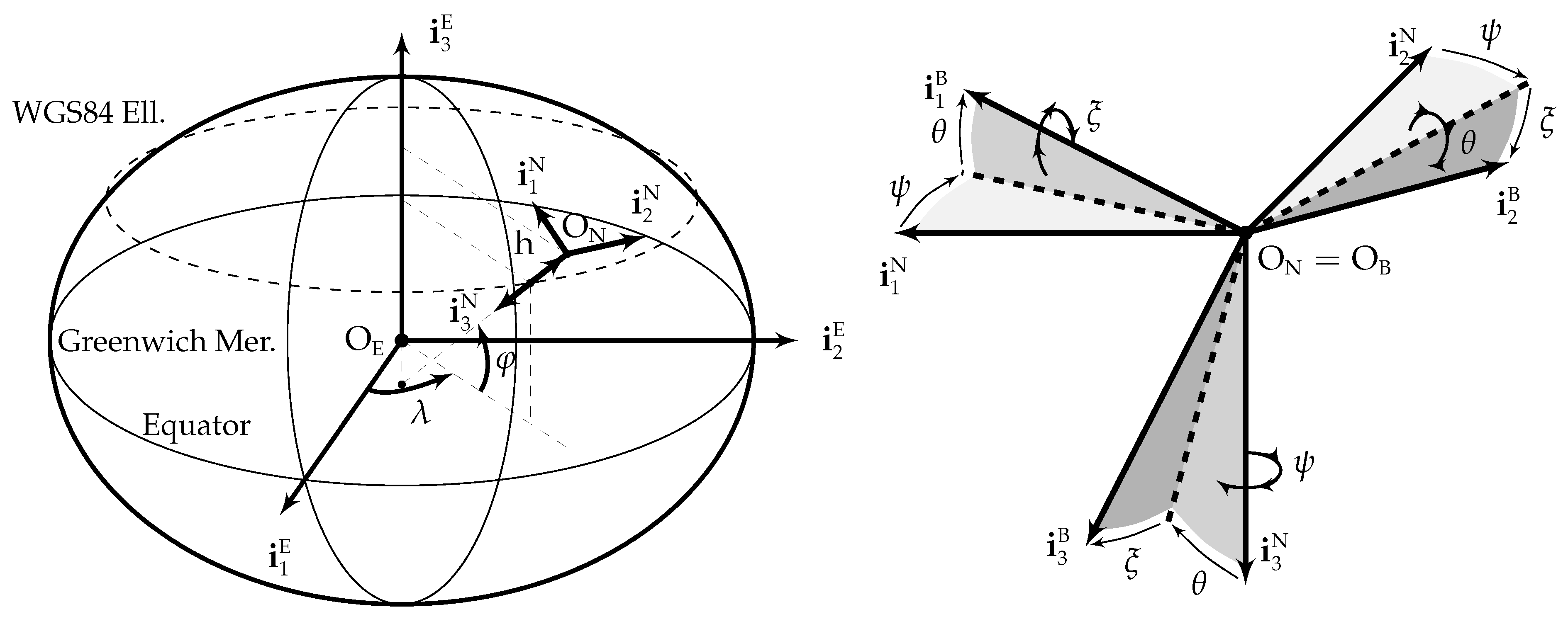
Five different reference frames are employed in this article: the ECEF frame ${\displaystyle {\mathrm{F}}_{\mathrm{E}}}$ (centered at the Earth center of mass ${\displaystyle {\mathrm{O}}_{\mathrm{E}}}$, with ${\displaystyle {\mathbf{i}}_3^{\mathrm{E}}}$ pointing towards the geodetic North along the Earth rotation axis, ${\displaystyle {\mathbf{i}}_1^{\mathrm{E}}}$ contained in both the Equator and zero longitude planes, and ${\displaystyle {\mathbf{i}}_2^{\mathrm{E}}}$ orthogonal to ${\displaystyle {\mathbf{i}}_1^{\mathrm{E}}}$ and ${\displaystyle {\mathbf{i}}_3^{\mathrm{E}}}$ forming a right handed system), the NED frame ${\displaystyle {\mathrm{F}}_{\mathrm{N}}}$ (centered at the aircraft center of mass ${\displaystyle {\mathrm{O}}_{\mathrm{N}}}$, with axes aligned with the geodetic North, East, and Down directions), the body frame ${\displaystyle {\mathrm{F}}_{\mathrm{B}}}$ (centered at the aircraft center of mass ${\displaystyle {\mathrm{O}}_{\mathrm{B}}={\mathrm{O}}_{\mathrm{N}}}$, with ${\displaystyle {\mathbf{i}}_1^{\mathrm{B}}}$ contained in the plane of symmetry of the aircraft pointing forward along a fixed direction, ${\displaystyle {\mathbf{i}}_3^{\mathrm{B}}}$ contained in the plane of symmetry of the aircraft, normal to ${\displaystyle {\mathbf{i}}_1^{\mathrm{B}}}$ and pointing downward, and ${\displaystyle {\mathbf{i}}_2^{\mathrm{B}}}$ 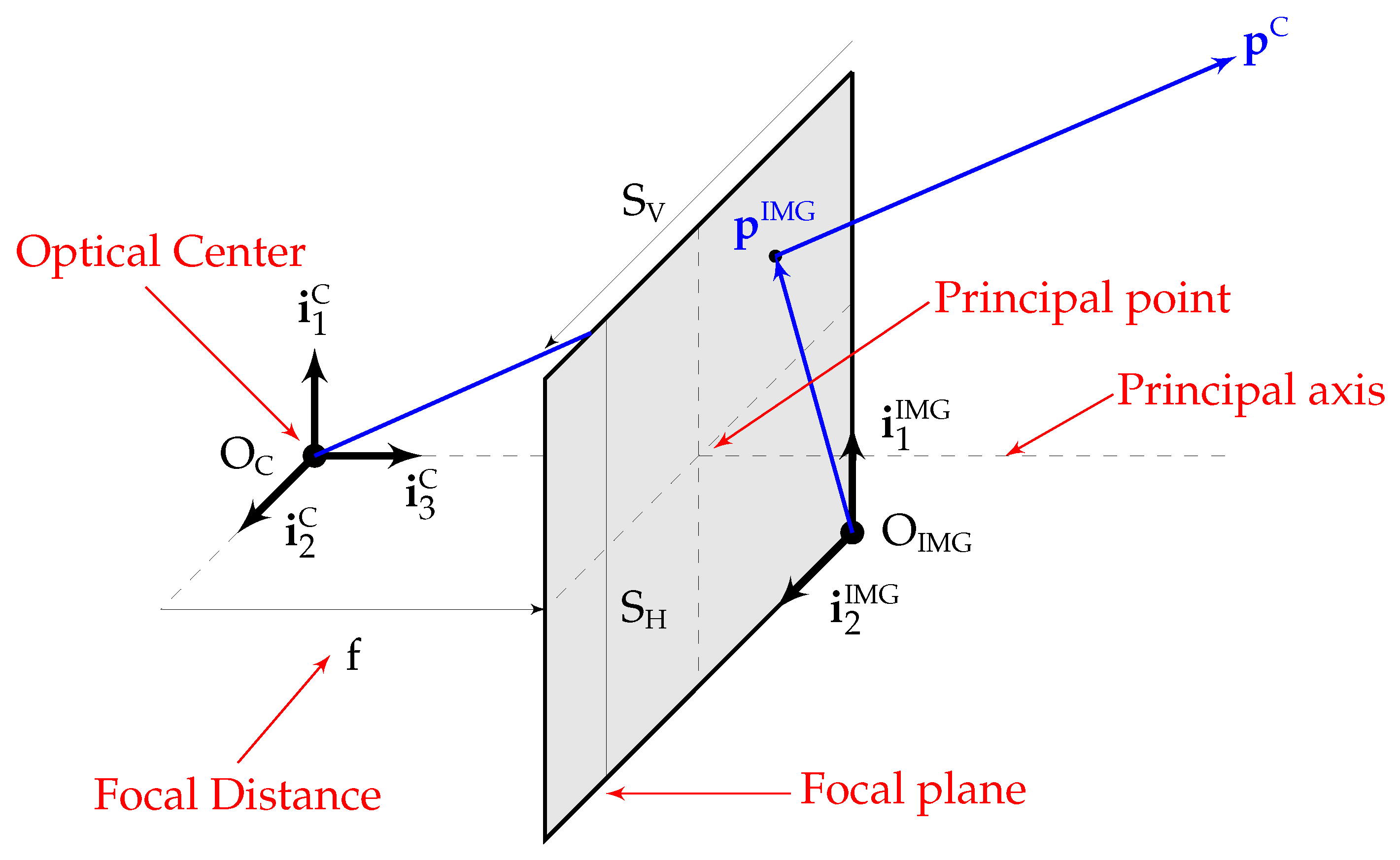orthogonal to both in such a way that they form a right hand system), the camera frame ${\displaystyle {\mathrm{F}}_{\mathrm{C}}}$ (centered at the optical center ${\displaystyle {\mathrm{O}}_{\mathrm{C}}}$, defined in Appendix A, with ${\displaystyle {\mathbf{i}}_3^{\mathrm{C}}}$ located in the camera principal axis pointing forward, and ${\displaystyle {\mathbf{i}}_1^{\mathrm{C}},{\mathbf{i}}_2^{\mathrm{C}}}$ parallel to the focal plane), and the image frame ${\displaystyle {\mathrm{F}}_{\mathrm{IMG}}}$ (two-dimensional frame centered at the sensor corner with axes parallel to the sensor borders). The first three frames are graphically depicted in Figure 1, while ${\displaystyle {\mathrm{F}}_{\mathrm{C}}}$ and ${\displaystyle {\mathrm{F}}_{\mathrm{IMG}}}$ can be visualized in Appendix A.

Superindexes are employed over vectors to specify the reference frame in which they are viewed (e.g., ${\displaystyle {\mathbf{v}}^{\mathrm{N}}}$ refers to ground velocity viewed in ${\displaystyle {\mathrm{F}}_{\mathrm{N}}}$, while ${\displaystyle {\mathbf{v}}^{\mathrm{B}}}$ is the same vector but viewed in ${\displaystyle {\mathrm{F}}_{\mathrm{B}}}$). Subindexes may be employed to clarify the meaning of the variable or vector, such as in ${\displaystyle {\mathbf{v}}_{\mathrm{TAS}}}$ for air velocity instead of the ground velocity ${\displaystyle \mathbf{v}}$, in which case the subindex is either an acronym or its meaning is clearly explained when first introduced. Subindexes may also refer to a given component of a vector, e.g., ${\displaystyle {\mathrm{v}}_2^{\mathrm{N}}}$ refers to the second component of ${\displaystyle {\mathbf{v}}^{\mathrm{N}}}$. In addition, where two reference frames appear as subindexes to a vector, it means that the vector goes from the first frame to the second. For example, ${\displaystyle {\mathbf{\omega }}_{\mathrm{NB}}^{\mathrm{B}}}$ refers to the angular velocity from the ${\displaystyle {\mathrm{F}}_{\mathrm{N}}}$ frame to the ${\displaystyle {\mathrm{F}}_{\mathrm{B}}}$ frame viewed in ${\displaystyle {\mathrm{F}}_{\mathrm{B}}}$.

Table 1. Mathematical notation.

${\displaystyle {\mathit{\gamma }}_{\mathbf{TAS}}}$	Aerodynamic path angle	${\displaystyle \mathbf{g}}$	Lie group action (transformation)
${\displaystyle \delta }$	Error threshold	${\displaystyle \mathrm{h}}$	Geometric altitude
${\displaystyle {\mathbf{\delta }}_{\mathrm{CNTR}}}$	Throttle and control surfaces position	${\displaystyle {\mathrm{H}}_{\mathrm{P}}}$	Pressure altitude
${\displaystyle {\mathbf{\delta }}_{\mathrm{TARGET}}}$	Control targets	${\displaystyle \mathbf{I}}$	Camera image
${\displaystyle \mathit{\Delta }}$	Estimation error, increment	${\displaystyle \mathbf{J}}$	Jacobian
${\displaystyle \mathit{\Delta }\mathrm{p}}$	Atmospheric pressure offset	${\displaystyle \mathcal{M}}$	${\displaystyle \mathbb{SE}\left(3\right)}$ Lie group element
${\displaystyle \mathit{\Delta }\mathrm{T}}$	Atmospheric temperature offset	${\displaystyle \mathbf{p}}$	Point, feature
${\displaystyle \theta }$	Body pitch angle	${\displaystyle \mathbf{q}}$	Attitude, unit quaternion
${\displaystyle \lambda }$	Longitude	${\displaystyle \mathbf{r}}$	Attitude, rotation vector
${\displaystyle \mathbf{\zeta }}$	Pose, unit dual quaternion	${\displaystyle \mathbf{R}}$	Attitude, rotation matrix
${\displaystyle \mu }$	Mean or expected value	${\displaystyle \mathcal{R}}$	${\displaystyle \mathbb{SO}\left(3\right)}$ Lie group element
${\displaystyle \xi }$	Body bank angle	${\displaystyle {\mathrm{s}}_{\mathrm{PX}}}$	Pixel size
${\displaystyle \mathbf{\xi }}$	Motion (${\displaystyle \mathbb{SE}\left(3\right)}$) velocity or twist	${\displaystyle \mathrm{S}}$	Sensor dimension
${\displaystyle \Pi }$	Camera projection	${\displaystyle \mathrm{t}}$	Time
${\displaystyle {\varrho }_{\mathrm{TUK}}}$	Tukey error function	${\displaystyle \mathbf{T}}$	Displacement
${\displaystyle \sigma }$	Standard deviation	${\displaystyle {\mathbf{T}}^{\mathrm{E},\mathrm{GDT}}}$	Geodetic coordinates
${\displaystyle \mathbf{\tau }}$	Pose, transform vector	${\displaystyle \mathrm{v}}$	Speed
${\displaystyle \phi }$	Latitude	${\displaystyle \mathbf{v}}$	Velocity
${\displaystyle \mathbf{\varphi }}$	Attitude, Euler angles	${\displaystyle {\mathrm{w}}_{\mathrm{TUK}}}$	Tukey weight function
${\displaystyle \varnothing }$	Bearing	${\displaystyle \mathrm{x}}$	Horizontal distance
${\displaystyle \psi }$	Heading or body yaw angle	${\displaystyle \mathbf{x}}$	Position
${\displaystyle \mathbf{\omega }}$	Angular (${\displaystyle \mathbb{SO}\left(3\right)}$) velocity	${\displaystyle \widehat{\mathbf{x}}={\mathbf{x}}_{\mathrm{EST}}}$	Inertial estimated trajectory
${\displaystyle {\mathrm{E}}_{\mathrm{PO}}}$	Pose optimization error	${\displaystyle \stackrel{\circ }{\mathbf{x}}={\mathbf{x}}_{\mathrm{IMG}}}$	Visual estimated trajectory
${\displaystyle {\mathrm{E}}_{\mathrm{q}}}$	Attitude adjustment error	${\displaystyle {\mathbf{x}}_{\mathrm{REF}}}$	Reference objectives
${\displaystyle {\mathrm{E}}_{\mathrm{RP}}}$	Reprojection error	${\displaystyle \tilde{\mathbf{x}}={\mathbf{x}}_{\mathrm{SENSED}}}$	Sensed trajectory
${\displaystyle \mathrm{f}}$	Focal length	${\displaystyle \mathbf{x}={\mathbf{x}}_{\mathrm{TRUTH}}}$	Real trajectory

summarizes the notation employed in this article.

In addition, there exist various indexes that appear as subindexes: n identifies a discrete time instant (${\displaystyle {\mathrm{t}}_{\mathrm{n}}}$) for the inertial estimations, s (${\displaystyle {\mathrm{t}}_{\mathrm{s}}}$) refers to the sensor outputs, i identifies an image or frame (${\displaystyle {\mathrm{t}}_{\mathrm{i}}}$), and k is employed for the keyframes used to generate the map or terrain structure. Other employed subindexes are l for the steps of the various iteration processes that take place, and j for the features and associated 3D points. With respect to superindexes, two stars ${\displaystyle <{·}^{🟉🟉}>}$ represent the reprojection only solution, while two circles ${\displaystyle <{·}^{\circ \circ }>}$ identify a target.

2. Introduction and Outline

This article focuses on the need to develop navigation systems capable of diminishing the position drift inherent to the flight in GNSS (Global Navigation Satellite System)-Denied conditions of an autonomous fixed wing aircraft so it has a higher probability of reaching the vicinity of a recovery point, from where it can be landed by remote control.

The article proposes a method that employs the inertial navigation outputs to improve the accuracy of VO (Visual Odometry) algorithms, which rely on the images of the Earth surface provided by a down looking camera rigidly attached to the aircraft structure, resulting in major improvements in horizontal position estimation accuracy over what can be achieved by standalone inertial or visual navigation systems. In contrast with most visual inertial methods found in the literature, which focus on short term GNSS-Denied navigation of ground vehicles, robots, and multi-rotors, the proposed algorithms are primarily intended for the long distance GNSS-Denied navigation of autonomous fixed wing aircraft.

Section 3 describes the article objectives, novelty, and main applications. When processing a new image, VO pipelines include a distinct phase known as pose optimization, pose refinement, or motion-only bundle adjustment, which estimates the camera pose (position plus attitude) based on previously estimated positions for the identified terrain features, both as ECEF 3D coordinates, as well as 2D coordinates of their projected location in the current image. Section 4 reviews the pose optimization algorithm when part of a standalone visual navigation system that can only rely on periodically generated images, while Section 5 proposes improvements to take advantage of the availability of aircraft pose estimations provided by an inertial navigation system.

Section 6 introduces the stochastic high-fidelity simulation employed to evaluate the navigation results by means of Monte Carlo executions of two scenarios representative of the challenges of GNSS-Denied navigation. The results obtained when applying the proposed algorithms to these two GNSS-Denied scenarios are described in Section 7, comparing them with those achieved by standalone inertial and visual systems. Section 8 discusses the sensitivity of the estimations to the type of terrain overflown by the aircraft, as the terrain texture (or lack of) and its elevation relief are key factors on the ability of the visual algorithms to detect and track terrain features. Last, the results are summarized for convenience in Section 9, while Section 10 provides a short conclusion.

Following a list of acronyms, the article concludes with three appendices. Appendix A provides a detailed description of the concept of optical flow, which is indispensable for the pose optimization algorithms of Section 4 and Section 5. Appendix B contains an introduction to GNSS-Denied navigation and its challenges, together with reviews of the state-of-the-art in two of the most promising routes to diminish its negative effects, such as visual odometry (VO) and visual inertial odometry (VIO). Last, Appendix C describes the different algorithms within Semi-Direct Visual Odometry (SVO) [4,5], a publicly available VO pipeline employed in this article, both by itself in Section 4 when relying exclusively on the images, and in the proposed improvements of Section 5 taking advantage of the inertial estimations.

3. Objective, Novelty, and Application

The main objective of this article is to improve the GNSS-Denied navigation capabilities of autonomous aircraft, so in case GNSS signals become unavailable, they can continue their mission or safely fly to a predetermined recovery location. To do so, the proposed approach combines two different navigation algorithms, employing the outputs of an INS (Inertial Navigation System) specifically designed for the flight without GNSS signals of an autonomous fixed wing low SWaP (Size, Weight, and Power) aircraft [6] to diminish the horizontal position drift generated by a VNS (Visual Navigation System) that relies on an advanced visual odometry pipeline, such as SVO [4,5]. Note that the INS makes use of all onboard sensors except the camera, while the VNS relies exclusively on the images provided by the camera.

As shown in Section 7, each of the two systems by itself incurs in unrestricted and excessive horizontal position drift that renders them inappropriate for long term GNSS-Denied navigation, but for different reasons: while in the INS the drift is the result of integrating the bounded ground velocity estimations without absolute position observations, that of the VNS originates on the slow but continuous accumulation of estimation errors between consecutive frames. The two systems however differ in their estimations of the aircraft attitude and altitude, as they are bounded for the INS but also drift in the case of the VNS. The proposed approach modifies the VNS so in addition to the images it can also accept as inputs the INS bounded attitude and altitude outputs, converting it into an Inertially Assisted VNS or IA-VNS with vastly improved horizontal position estimation capabilities.

The VIO solutions listed in Appendix B are quite generic with respect to the platforms on which they are mounted, with most applications focused on ground vehicles, indoor robots, and multi-rotors, as well as with respect to the employed sensors, which are usually restricted to the gyroscopes and accelerometers, together with one or more cameras. This article focuses on an specific case (long distance GNSS-Denied turbulent flight of fixed wing aircraft), and, as such, is simultaneously more restrictive but also takes advantage of the sensors already present onboard these platforms, such as magnetometers, Pitot tube, and air vanes. In addition, and unlike the existing VIO packages, the proposed solution assumes that GNSS signals are present at the beginning of the flight. As described in detail in [6], these are key to the obtainment of the bounded attitude and altitude INS outputs on which the proposed IA-VNS relies.

The proposed method represents a novel approach to diminish the pose drift of a VO pipeline by supplementing its pose estimation non-linear optimizations with priors based on the bounded attitude and altitude outputs of a GNSS-Denied inertial filter. The method is inspired in a PI (Proportional Integral) control loop, in which the inertial attitude and altitude outputs act as targets to ensure that the visual estimations do not deviate in excess from their inertial counterparts, resulting in major reductions to not only the visual attitude and altitude estimation errors, but also to the drift in horizontal position.

This article proves that inertial and visual navigation systems can be combined in such a way that the resulting long term GNSS-Denied horizontal position drift is significantly smaller than what can be obtained by either system individually. In the case that GNSS signals become unavailable in mid flight, GNSS-Denied navigation is required for the platform to complete its mission or return to base without the absolute position and ground velocity observations provided by GNSS receivers. As shown in the following sections, the proposed system can significantly increase the possibilities of the aircraft safely reaching the vicinity of the intended recovery location, from where it can be landed by remote control.

4. Pose Optimization within Visual Odometry

Visual navigation, also known as visual odometry or VO, relies on images of the Earth’s surface generated by an onboard camera to incrementally estimate the aircraft pose (position plus attitude) based on the changes that its motion induces on the images, without the assistance of image databases or the observations of any other onboard sensors. As it does not rely on GNSS signals, it is considered an alternative to GNSS-Denied inertial navigation, although it also incurs in an unrestricted horizontal position drift. Appendix B.2 provides an overview of various VO pipelines within the broader context of the problems associated to GNSS-Denied navigation and the research paths most likely to diminish them (Appendix B).

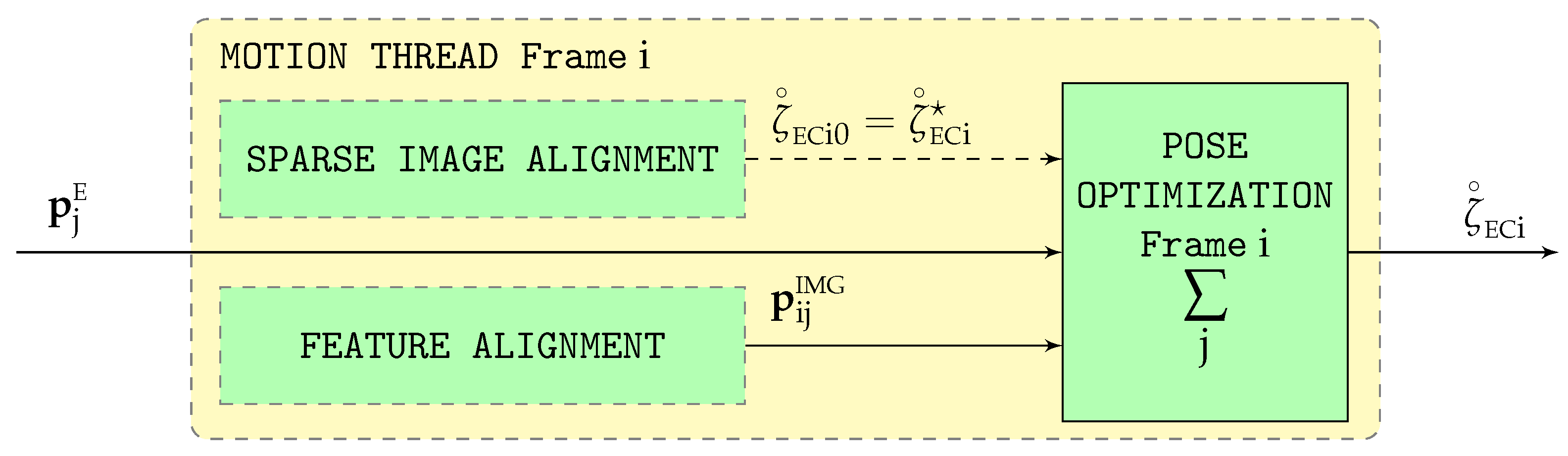
This article employs SVO (Semi-Direct Visual Odometry) [4,5], a state-of-the-art publicly available VO pipeline, as a baseline on which to apply the proposed improvements based on the availability of inertial estimations of the aircraft pose. Although Appendix C describes the various threads and processes within SVO, the focus of the proposed improvements within Section 5 lies in the pose optimization phase, which is the only one described in detail in this article. Note that other VO pipelines also make use of similar pose optimization algorithms.

Graphically depicted in Figure 2, pose optimization is executed for every new frame i and estimates the pose between the ECEF (${\displaystyle {\mathrm{F}}_{\mathrm{E}}}$) and camera (${\displaystyle {\mathrm{F}}_{\mathrm{C}}}$) frames (${\displaystyle {\stackrel{\circ }{\mathbf{\zeta }}}_{\mathrm{EC}\mathrm{i}}}$). It requires the following inputs:

• The ECEF terrain 3D coordinates of all features j visible in the image (${\displaystyle {\mathbf{p}}_{\mathrm{j}}^{\mathrm{E}}}$) obtained by the structure optimization phase (Appendix C) corresponding to the previous image. These terrain 3D coordinates are known as the terrain map, and constitute a side product generated by VO pipelines.
• The 2D position of the same features j within the current image i (${\displaystyle {\mathbf{p}}_{\mathrm{ij}}^{\mathrm{IMG}}}$) supplied by the previous feature alignment phase (Appendix C).
• The rough estimation of the ECEF to camera pose ${\displaystyle {\stackrel{\circ }{\mathbf{\zeta }}}_{\mathrm{EC}\mathrm{i}}^{🟉}}$ for the current frame i provided by the sparse image alignment phase (Appendix C), which acts as the initial value for the camera pose (${\displaystyle {\stackrel{\circ }{\mathbf{\zeta }}}_{\mathrm{EC}\mathrm{i}0}}$) to be refined by iteration.

The pose optimization algorithm, also known as pose refinement or motion-only bundle adjustment, estimates the camera pose by minimizing the reprojection error of the different features. Pose optimization relies exclusively on the information obtained from the images generated by the onboard camera, and is described in detail to act as a baseline on which to apply in Section 5 the proposed improvements enabled by the availability of additional pose estimations generated by an inertial navigation system or INS.

The reprojection error ${\displaystyle {\mathrm{E}}_{\mathrm{RPi}}}$, a function of the estimated ECEF to camera pose for image i (${\displaystyle {\stackrel{\circ }{\mathbf{\zeta }}}_{\mathrm{EC}\mathrm{i}}}$), is defined in (1) as the sum for each feature terrain 3D point j of the norm of the difference between the camera projection ${\displaystyle \mathit{\Pi }}$ of the ECEF coordinates ${\displaystyle {\mathbf{p}}_{\mathrm{j}}^{\mathrm{E}}}$ transformed into the camera frame and the image coordinates ${\displaystyle {\mathbf{p}}_{\mathrm{j}}^{\mathrm{IMG}}}$. Note that ${\displaystyle {\mathbf{g}}_{{\displaystyle {\mathbf{\zeta }}_{\mathrm{AB}}}}()}$ represents the ${\displaystyle \mathbb{SE}\left(3\right)}$ transformation of a point from frame B to frame A, as described in [1], and the camera projection ${\displaystyle \mathit{\Pi }}$ is defined in Appendix A.

$${\mathrm{E}}_{\mathrm{RPi}}\left({\stackrel{\circ }{\mathbf{\zeta }}}_{\mathrm{EC}\mathrm{i}}\right)={\displaystyle \sum _{\mathrm{j}}}\parallel \mathit{\Pi }\left({\mathbf{g}}_{{\displaystyle {\stackrel{\circ }{\mathbf{\zeta }}}_{\mathrm{EC}\mathrm{i}}}}^{-1}\left({\mathbf{p}}_{\mathrm{j}}^{\mathrm{E}}\right)\right)-{\mathbf{p}}_{\mathrm{ij}}^{\mathrm{IMG}}\parallel$$

(1)

This problem can be solved by means of an iterative Gauss-Newton gradient descent process [1,7]. Given an initial camera pose estimation ${\displaystyle {\stackrel{\circ }{\mathbf{\zeta }}}_{\mathrm{EC}\mathrm{i}0}}$ taken from the sparse image alignment result (${\displaystyle {\stackrel{\circ }{\mathbf{\zeta }}}_{\mathrm{EC}\mathrm{i}}^{🟉}}$, Figure 2), each iteration step l minimizes (2) and advances the estimated solution by means of (3) until the step diminution of the reprojection error falls below a given threshold ${\displaystyle {\delta }_{\mathrm{RP}}}$${\displaystyle \left({\mathrm{E}}_{\mathrm{RP},\mathrm{i},\mathrm{l}}-{\mathrm{E}}_{\mathrm{RP},\mathrm{i},\mathrm{l}+1}<{\delta }_{\mathrm{RP}}\right)}$. Note that ${\displaystyle \mathit{\Delta }{\stackrel{\circ }{\mathbf{\tau }}}_{\mathrm{EC}\mathrm{il}}^{\mathrm{C}}}$ represents the estimated tangent space incremental ECEF to camera pose (transform vector) viewed in the ${\displaystyle {\mathrm{F}}_{\mathrm{C}}}$ camera frame for image i and iteration l, ${\displaystyle \oplus }$ and ${\displaystyle \circ }$ represent the ${\displaystyle \mathbb{SE}\left(3\right)}$ plus and concatenation operators, and ${\displaystyle \mathrm{Exp}\left(\right)}$ refers to the ${\displaystyle \mathbb{SE}\left(3\right)}$ capitalized exponential function [1,3]. Additionally, note that, while ${\displaystyle {\mathrm{E}}_{\mathrm{RPi}}}$ and ${\displaystyle {\mathrm{E}}_{\mathrm{RPi},\mathrm{l}+1}}$ present in (1) and (2) are both positive scalars, the feature j reprojection error ${\displaystyle {\mathbf{E}}_{\mathrm{RPi},\mathrm{l}+1,\mathrm{j}}}$ that appears in (2) is an ${\displaystyle {\mathbb{R}}^3}$ vector.

$$\begin{array}{ccc}\hfill {\mathrm{E}}_{\mathrm{RPi},\mathrm{l}+1}\left(\mathit{\Delta }{\stackrel{\circ }{\mathbf{\tau }}}_{\mathrm{EC}\mathrm{il}}^{\mathrm{C}}\right)& =& {\displaystyle \sum _{\mathrm{j}}}\parallel \mathit{\Pi }\left({\mathbf{g}}_{{\displaystyle {\stackrel{\circ }{\mathbf{\zeta }}}_{\mathrm{EC}\mathrm{il}}\oplus \mathit{\Delta }{\stackrel{\circ }{\mathbf{\tau }}}_{\mathrm{EC}\mathrm{il}}^{\mathrm{C}}}}^{-1}\left({\mathbf{p}}_{\mathrm{j}}^{\mathrm{E}}\right)\right)-{\mathbf{p}}_{\mathrm{ij}}^{\mathrm{IMG}}\parallel ={\displaystyle \sum _{\mathrm{j}}}\parallel {\mathbf{E}}_{\mathrm{RPi},\mathrm{l}+1,\mathrm{j}}\left(\mathit{\Delta }{\stackrel{\circ }{\mathbf{\tau }}}_{\mathrm{EC}\mathrm{il}}^{\mathrm{C}}\right)\parallel \hfill \end{array}$$

(2)

$$\begin{array}{ccc}\hfill {\stackrel{\circ }{\mathbf{\zeta }}}_{\mathrm{EC}\mathrm{i},\mathrm{l}+1}& ⟵& {\stackrel{\circ }{\mathbf{\zeta }}}_{\mathrm{EC}\mathrm{il}}\circ \mathrm{Exp}\left(\mathit{\Delta }{\stackrel{\circ }{\mathbf{\tau }}}_{\mathrm{EC}\mathrm{il}}^{\mathrm{C}}\right)={\stackrel{\circ }{\mathbf{\zeta }}}_{\mathrm{EC}\mathrm{il}}\oplus \mathit{\Delta }{\stackrel{\circ }{\mathbf{\tau }}}_{\mathrm{EC}\mathrm{il}}^{\mathrm{C}}\hfill \end{array}$$

(3)

Each ${\displaystyle \mathit{\Delta }{\stackrel{\circ }{\mathbf{\tau }}}_{\mathrm{EC}\mathrm{il}}^{\mathrm{C}}}$ represents the update to the camera pose ${\displaystyle {\stackrel{\circ }{\mathbf{\zeta }}}_{\mathrm{EC}\mathrm{il}}}$ viewed in the local camera frame ${\displaystyle {\mathrm{F}}_{\mathrm{C}\mathrm{il}}}$, which is obtained by following the process described in [1,7], and results in (4), where ${\displaystyle {\mathbf{J}}_{\mathrm{OF},\mathrm{ilj}}}$ (5) is the optical flow for image i, iteration step l, and feature j obtained in Appendix A:

$$\begin{array}{ccc}\hfill \mathit{\Delta }{\stackrel{\circ }{\mathbf{\tau }}}_{\mathrm{EC}\mathrm{il}}^{\mathrm{C}}& =& -{\left[{\displaystyle \sum _{\mathrm{j}}}{{\mathbf{J}}_{\mathrm{OF},\mathrm{ilj}}}^{\mathrm{T}}{\mathbf{J}}_{\mathrm{OF},\mathrm{ilj}}\right]}^{-1}{\displaystyle \sum _{\mathrm{j}}}{{\mathbf{J}}_{\mathrm{OF},\mathrm{ilj}}}^{\mathrm{T}}\left[\mathit{\Pi }\left({\mathbf{g}}_{{\displaystyle {\stackrel{\circ }{\mathbf{\zeta }}}_{\mathrm{EC}\mathrm{il}}}}^{-1}\left({\mathbf{p}}_{\mathrm{j}}^{\mathrm{E}}\right)\right)-{\mathbf{p}}_{\mathrm{ij}}^{\mathrm{IMG}}\right]\in {\mathbb{R}}^6\hfill \end{array}$$

(4)

$$\begin{array}{ccc}\hfill {\mathbf{J}}_{\mathrm{OF},\mathrm{ilj}}& =& {\mathbf{J}}_{\mathrm{OF}}\left(\mathit{\Pi }\right({\mathbf{g}}_{{\stackrel{\circ }{\mathbf{\zeta }}}_{\mathrm{EC}\mathrm{il}}}^{-1}\left({\mathbf{p}}_{\mathrm{j}}^{\mathrm{E}}\right)\left)\right)\in {\mathbb{R}}^{2\times 6}\hfill \end{array}$$

(5)

In order to protect the resulting pose from the possible presence of outliers in either the feature terrain 3D points ${\displaystyle {\mathbf{p}}_{\mathrm{j}}^{\mathrm{E}}}$ or their image projections ${\displaystyle {\mathbf{p}}_{\mathrm{ij}}^{\mathrm{IMG}}}$, it is better to replace the above squared error or mean estimator by a more robust M-estimator, such as the bisquare or Tukey estimator [8,9]. The error to be minimized in each iteration step is then given by (6), where the Tukey error function ${\displaystyle {\varrho }_{\mathrm{TUK}}\left(\mathrm{x}\right)}$ can be found in [9].

$$\begin{array}{ccc}\hfill {\mathrm{E}}_{\mathrm{RPi},\mathrm{l}+1}\left(\mathit{\Delta }{\stackrel{\circ }{\mathbf{\tau }}}_{\mathrm{EC}\mathrm{il}}^{\mathrm{C}}\right)& =& {\displaystyle \sum _{\mathrm{j}}}{\varrho }_{\mathrm{TUK}}\left({\left[\mathit{\Pi }\left({\mathbf{g}}_{{\displaystyle {\stackrel{\circ }{\mathbf{\zeta }}}_{\mathrm{EC}\mathrm{il}}\oplus \mathit{\Delta }{\stackrel{\circ }{\mathbf{\tau }}}_{\mathrm{EC}\mathrm{il}}^{\mathrm{C}}}}^{-1}\left({\mathbf{p}}_{\mathrm{j}}^{\mathrm{E}}\right)\right)-{\mathbf{p}}_{\mathrm{ij}}^{\mathrm{IMG}}\right]}^{\mathrm{T}}\left[\mathit{\Pi }\left({\mathbf{g}}_{{\displaystyle {\stackrel{\circ }{\mathbf{\zeta }}}_{\mathrm{EC}\mathrm{il}}\oplus \mathit{\Delta }{\stackrel{\circ }{\mathbf{\tau }}}_{\mathrm{EC}\mathrm{il}}^{\mathrm{C}}}}^{-1}\left({\mathbf{p}}_{\mathrm{j}}^{\mathrm{E}}\right)\right)-{\mathbf{p}}_{\mathrm{ij}}^{\mathrm{IMG}}\right]\right)\hfill \\ & =& {\displaystyle \sum _{\mathrm{j}}}{\varrho }_{\mathrm{TUK}}\left({{\mathbf{E}}_{\mathrm{RPi},\mathrm{l}+1,\mathrm{j}}}^{\mathrm{T}}{\mathbf{E}}_{\mathrm{RPi},\mathrm{l}+1,\mathrm{j}}\right)\hfill \end{array}$$

(6)

A similar process to that employed above leads to the solution (7), where the Tukey weight function ${\displaystyle {\mathrm{w}}_{\mathrm{TUK}}\left(\mathrm{x}\right)}$ is also provided by [9]:

$$\begin{array}{ccc}\hfill \mathit{\Delta }{\stackrel{\circ }{\mathbf{\tau }}}_{\mathrm{EC}\mathrm{il}}^{\mathrm{C}}& =& -{\left[{\displaystyle \sum _{\mathrm{j}}}{\mathrm{w}}_{\mathrm{TUK}}\left({{\mathbf{E}}_{\mathrm{RP},\mathrm{ilj}}}^{\mathrm{T}}{\mathbf{E}}_{\mathrm{RP},\mathrm{ilj}}\right){{\mathbf{J}}_{\mathrm{OF},\mathrm{ilj}}}^{\mathrm{T}}{\mathbf{J}}_{\mathrm{OF},\mathrm{ilj}}\right]}^{-1}\hfill \\ & & \left[{\displaystyle \sum _{\mathrm{j}}}{\mathrm{w}}_{\mathrm{TUK}}\left({{\mathbf{E}}_{\mathrm{RP},\mathrm{ilj}}}^{\mathrm{T}}{\mathbf{E}}_{\mathrm{RP},\mathrm{ilj}}\right){{\mathbf{J}}_{\mathrm{OF},\mathrm{ilj}}}^{\mathrm{T}}{\mathbf{E}}_{\mathrm{RP},\mathrm{ilj}}\right]\in {\mathbb{R}}^6\hfill \end{array}$$

(7)

$$\begin{array}{ccc}\hfill {\mathbf{E}}_{\mathrm{RP},\mathrm{ilj}}& =& \mathit{\Pi }\left({\mathbf{g}}_{{\displaystyle {\stackrel{\circ }{\mathbf{\zeta }}}_{\mathrm{EC}\mathrm{il}}}}^{-1}\left({\mathbf{p}}_{\mathrm{j}}^{\mathrm{E}}\right)\right)-{\mathbf{p}}_{\mathrm{ij}}^{\mathrm{IMG}}\in {\mathbb{R}}^2\hfill \end{array}$$

(8)

5. Proposed Pose Optimization within Visual Inertial Odometry

Lacking any absolute references, all visual odometry (VO) pipelines gradually accumulate errors in each of the six dimensions of the estimated ECEF to vehicle body pose ${\displaystyle {\stackrel{\circ }{\mathbf{\zeta }}}_{\mathrm{EB}}}$. The resulting estimation error drift is described in Section 7 for the specific case of SVO, which is introduced in Appendix C, and whose pose optimization phase is described in Section 4.

This article proposes a method to improve the pose estimation capabilities of visual odometry pipelines by supplementing them with the outputs provided by an inertial navigation system. Taking the pose optimization algorithm of SVO (Section 4) as a baseline, this section describes the proposed improvements, while Section 7 explains the results obtained when applying the algorithms to two scenarios representative of GNSS-Denied navigation (Section 6).

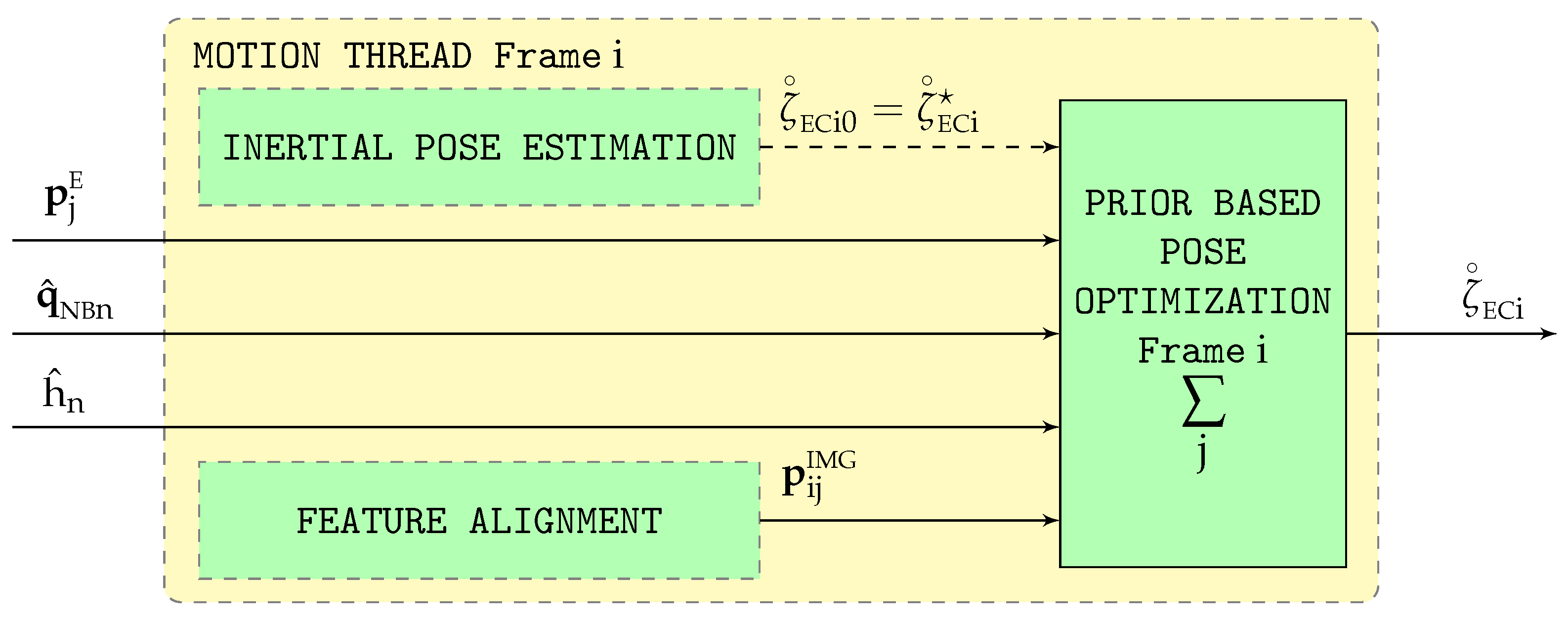
If accurate estimations of attitude and altitude can be provided by an inertial navigation system (INS) such as that described in [6], these can be employed to ensure that the visual estimations for body attitude and vertical position (${\displaystyle {\stackrel{\circ }{\mathbf{q}}}_{\mathrm{NB}}}$ and ${\displaystyle \stackrel{\circ }{\mathrm{h}}}$, part of the body pose ${\displaystyle {\stackrel{\circ }{\mathbf{\zeta }}}_{\mathrm{EB}}}$) do not deviate in excess from their inertial counterparts ${\displaystyle {\widehat{\mathbf{q}}}_{\mathrm{NB}}}$ and ${\displaystyle \widehat{\mathrm{h}}}$, improving their accuracy. This process is depicted in Figure 3.

The inertial estimations (${\displaystyle {\widehat{\mathbf{q}}}_{\mathrm{NB}},\widehat{\mathrm{h}}}$) should not replace the visual ones (${\displaystyle {\stackrel{\circ }{\mathbf{q}}}_{\mathrm{NB}},\stackrel{\circ }{\mathrm{h}}}$) within SVO, as this would destabilize the visual pipeline preventing its convergence, but just act as anchors so the visual estimations oscillate freely as a result of the multiple SVO optimizations but without drifting from the vicinity of the anchors. This section shows how to modify the cost function within the iterative Gauss-Newton gradient descent pose optimization phase (Section 4) so it can take advantage of the inertial outputs. It is necessary to remark that, as indicated in Section 6, the inertial estimations (denoted by the subindex n) operate at a much higher rate than the visual ones (denoted by the subindex i).

5.1. Rationale for the Introduction of Priors

The prior based pose optimization process starts by executing exactly the same pose optimization described in Section 4, which seeks to obtain the ECEF to camera pose ${\displaystyle {\stackrel{\circ }{\mathbf{\zeta }}}_{\mathrm{EC}\mathrm{i}}}$ that minimizes the reprojection error ${\displaystyle {\mathrm{E}}_{\mathrm{RPi}}}$ (1). The iterative optimization results in a series of ${\displaystyle \mathbb{SE}\left(3\right)}$ tangent space updates ${\displaystyle \mathit{\Delta }{\stackrel{\circ }{\mathbf{\tau }}}_{\mathrm{EC}\mathrm{il}}^{\mathrm{C}}}$ (7), where i identifies the image and l indicates the iteration step. The camera pose is then advanced per (3) until the step diminution of the reprojection error falls below a certain threshold ${\displaystyle {\delta }_{\mathrm{RP}}}$.

The resulting ECEF to camera pose, ${\displaystyle {\stackrel{\circ }{\mathbf{\zeta }}}_{\mathrm{EC}\mathrm{i}}}$, is marked with the superindex ${\displaystyle 🟉🟉}$ to indicate that it is the reprojection only solution, resulting in ${\displaystyle {\stackrel{\circ }{\mathbf{\zeta }}}_{\mathrm{EC}\mathrm{i}}^{🟉🟉}}$. Its concatenation with the constant body to camera pose ${\displaystyle {\mathbf{\zeta }}_{\mathrm{BC}}}$ results in the reprojected ECEF to body pose ${\displaystyle {\stackrel{\circ }{\mathbf{\zeta }}}_{\mathrm{EB}\mathrm{i}}^{🟉🟉}}$ (note that a single asterisk superindex ${\displaystyle <{·}^{\ast }>}$ applied to a pose refers to its conjugate or inverse, and that the concatenation ${\displaystyle \circ }$ and multiplication ${\displaystyle \otimes }$ operators are equivalent for ${\displaystyle \mathbb{SE}\left(3\right)}$ rigid body poses):

$${\stackrel{\circ }{\mathbf{\zeta }}}_{\mathrm{EB}\mathrm{i}}^{🟉🟉}={\stackrel{\circ }{\mathbf{\zeta }}}_{\mathrm{EC}\mathrm{i}}^{🟉🟉}\circ {\mathbf{\zeta }}_{\mathrm{BC}}^{\ast }={\stackrel{\circ }{\mathbf{\zeta }}}_{\mathrm{EC}\mathrm{i}}^{🟉🟉}\otimes {\mathbf{\zeta }}_{\mathrm{BC}}^{\ast }={\stackrel{\circ }{\mathbf{\zeta }}}_{\mathrm{EC}\mathrm{i}}^{🟉🟉}\otimes {\mathbf{\zeta }}_{\mathrm{CB}}$$

(9)

The reprojected ECEF to body attitude ${\displaystyle {\stackrel{\circ }{\mathbf{q}}}_{\mathrm{EB}\mathrm{i}}^{🟉🟉}}$ and Cartesian coordinates ${\displaystyle {\stackrel{\circ }{\mathbf{T}}}_{\mathrm{EB}\mathrm{i}}^{\mathrm{B}🟉🟉}}$ can then be readily obtained from ${\displaystyle {\stackrel{\circ }{\mathbf{\zeta }}}_{\mathrm{EB}\mathrm{i}}^{🟉🟉}}$, which leads on one hand to the reprojected NED to body attitude ${\displaystyle {\stackrel{\circ }{\mathbf{q}}}_{\mathrm{NB}\mathrm{i}}^{🟉🟉}}$, equivalent to the Euler angles ${\displaystyle {\stackrel{\circ }{\mathbf{\varphi }}}_{\mathrm{NB}\mathrm{i}}^{🟉🟉}={\left[{\stackrel{\circ }{\psi }}_{\mathrm{i}}^{🟉🟉},{\stackrel{\circ }{\theta }}_{\mathrm{i}}^{🟉🟉},{\stackrel{\circ }{\xi }}_{\mathrm{i}}^{🟉🟉}\right]}^{\mathrm{T}}}$ (yaw, pitch, and bank angles, respectively), and on the other to the geodetic coordinates ${\displaystyle {\stackrel{\circ }{\mathbf{T}}}_{\mathrm{i}}^{\mathrm{E},\mathrm{GDT}🟉🟉}={\left[{\stackrel{\circ }{\lambda }}_{\mathrm{i}}^{🟉🟉},{\stackrel{\circ }{\phi }}_{\mathrm{i}}^{🟉🟉},{\stackrel{\circ }{\mathrm{h}}}_{\mathrm{i}}^{🟉🟉}\right]}^{\mathrm{T}}}$ (longitude, latitude, and altitude) and ECEF to NED rotation ${\displaystyle {\stackrel{\circ }{\mathbf{q}}}_{\mathrm{EN}\mathrm{i}}^{🟉🟉}}$.

Let us assume for the time being that the inertially estimated body attitude (${\displaystyle {\widehat{\mathbf{q}}}_{\mathrm{NB}\mathrm{n}}}$) or altitude (${\displaystyle {\widehat{\mathrm{h}}}_{\mathrm{n}}}$) [6] enable the navigation system to conclude that it would be preferred if the visually optimized body attitude were closer to a certain target attitude identified by the superindex ${\displaystyle \circ \circ }$, ${\displaystyle {\stackrel{\circ }{\mathbf{q}}}_{\mathrm{NB}\mathrm{i}}^{\circ \circ }}$, equivalent to the target Euler angles ${\displaystyle {\stackrel{\circ }{\mathbf{\varphi }}}_{\mathrm{NB}\mathrm{i}}^{\circ \circ }={\left[{\stackrel{\circ }{\psi }}_{\mathrm{i}}^{\circ \circ },{\stackrel{\circ }{\theta }}_{\mathrm{i}}^{\circ \circ },{\stackrel{\circ }{\xi }}_{\mathrm{i}}^{\circ \circ }\right]}^{\mathrm{T}}}$. Section 5.3 specifies when this assumption can be considered valid, as well as various alternatives to obtain the target attitude from ${\displaystyle {\widehat{\mathbf{q}}}_{\mathrm{NB}\mathrm{n}}}$ and ${\displaystyle {\widehat{\mathrm{h}}}_{\mathrm{n}}}$. The target NED to body attitude ${\displaystyle {\stackrel{\circ }{\mathbf{q}}}_{\mathrm{NB}\mathrm{i}}^{\circ \circ }}$ is converted into a target ECEF to camera attitude ${\displaystyle {\stackrel{\circ }{\mathbf{q}}}_{\mathrm{EC}\mathrm{i}}^{\circ \circ }}$ by means of the constant body to camera rotation ${\displaystyle {\mathbf{q}}_{\mathrm{BC}}}$ and the original reprojected ECEF to NED rotation ${\displaystyle {\stackrel{\circ }{\mathbf{q}}}_{\mathrm{EN}\mathrm{i}}^{🟉🟉}}$, incurring in a negligible error by not considering the attitude change of the NED frame as the iteration progresses. The concatenation ${\displaystyle \circ }$ and multiplication ${\displaystyle \otimes }$ operators are equivalent for ${\displaystyle \mathbb{SO}\left(3\right)}$ rigid body rotations:

$${\stackrel{\circ }{\mathbf{q}}}_{\mathrm{EC}\mathrm{i}}^{\circ \circ }={\stackrel{\circ }{\mathbf{q}}}_{\mathrm{EN}\mathrm{i}}^{🟉🟉}\circ {\stackrel{\circ }{\mathbf{q}}}_{\mathrm{NB}\mathrm{i}}^{\circ \circ }\circ {\mathbf{q}}_{\mathrm{BC}}={\stackrel{\circ }{\mathbf{q}}}_{\mathrm{EN}\mathrm{i}}^{🟉🟉}\otimes {\stackrel{\circ }{\mathbf{q}}}_{\mathrm{NB}\mathrm{i}}^{\circ \circ }\otimes {\mathbf{q}}_{\mathrm{BC}}$$

(10)

Note that the objective is not for the resulting body attitude ${\displaystyle {\stackrel{\circ }{\mathbf{q}}}_{\mathrm{NB}\mathrm{i}}}$ to equal the target ${\displaystyle {\stackrel{\circ }{\mathbf{q}}}_{\mathrm{NB}\mathrm{i}}^{\circ \circ }}$, but to balance both objectives (minimization of the reprojection error of the various terrain 3D points and minimization of the attitude differences with the targets) without imposing any hard constraints on the pose (position plus attitude) of the aircraft.

5.2. Prior-Based Pose Optimization

The attitude adjustment error ${\displaystyle {\mathrm{E}}_{\mathrm{q},\mathrm{i}}}$, a function of the estimated ECEF to camera attitude for image i (${\displaystyle {\stackrel{\circ }{\mathbf{q}}}_{\mathrm{EC}\mathrm{i}}}$), is defined in (11) as the norm of the Euclidean difference between rotation vectors corresponding to the estimated and target ECEF to camera attitudes (${\displaystyle {\stackrel{\circ }{\mathbf{q}}}_{\mathrm{EC}\mathrm{i}},{\stackrel{\circ }{\mathbf{q}}}_{\mathrm{EC}\mathrm{i}}^{\circ \circ }}$) [1,3]. Note that ${\displaystyle \mathrm{Log}\left(\right)}$ refers to the ${\displaystyle \mathbb{SO}\left(3\right)}$ capitalized logarithmic function [1,3].

$${\mathrm{E}}_{\mathrm{q},\mathrm{i}}\left(\mathrm{Log}\left({\stackrel{\circ }{\mathbf{q}}}_{\mathrm{EC}\mathrm{i}}\right)\right)={\mathrm{E}}_{\mathrm{q},\mathrm{i}}\left({\stackrel{\circ }{\mathbf{r}}}_{\mathrm{EC}\mathrm{i}}\right)=\parallel \mathrm{Log}\left({\stackrel{\circ }{\mathbf{q}}}_{\mathrm{EC}\mathrm{i}}\right)-\mathrm{Log}\left({\stackrel{\circ }{\mathbf{q}}}_{\mathrm{EC}\mathrm{i}}^{\circ \circ }\right)\parallel =\parallel {\stackrel{\circ }{\mathbf{r}}}_{\mathrm{EC}\mathrm{i}}-{\stackrel{\circ }{\mathbf{r}}}_{\mathrm{EC}\mathrm{i}}^{\circ \circ }\parallel$$

(11)

Its minimization can be solved by means of an iterative Gauss-Newton gradient descent process [1,7]. Given an initial rotation vector (attitude) estimation ${\displaystyle {\stackrel{\circ }{\mathbf{r}}}_{\mathrm{EC}\mathrm{i},0}=\mathrm{Log}\left({\stackrel{\circ }{\mathbf{q}}}_{\mathrm{EC}\mathrm{i},0}\right)}$ taken from the initial pose ${\displaystyle {\stackrel{\circ }{\mathbf{\zeta }}}_{\mathrm{EC}\mathrm{i}0}={\stackrel{\circ }{\mathbf{\zeta }}}_{\mathrm{EC}\mathrm{i}}^{🟉}}$, each iteration step l minimizes (12) and advances the estimated solution by means of (3) until the step diminution of the attitude adjustment error falls below a given threshold ${\displaystyle {\delta }_{\mathrm{q}}}$${\displaystyle \left({\mathrm{E}}_{\mathrm{q},\mathrm{i},\mathrm{l}}-{\mathrm{E}}_{\mathrm{q},\mathrm{i},\mathrm{l}+1}<{\delta }_{\mathrm{q}}\right)}$. Note that ${\displaystyle \mathit{\Delta }{\stackrel{\circ }{\mathbf{r}}}_{\mathrm{EC}\mathrm{il}}^{\mathrm{C}}}$ represents the estimated tangent space incremental ECEF to camera attitude (rotation vector) viewed in the ${\displaystyle {\mathrm{F}}_{\mathrm{C}}}$ camera frame for image i and iteration l, ${\displaystyle \oplus }$ and ${\displaystyle \circ }$ represent the ${\displaystyle \mathbb{SO}\left(3\right)}$ plus and concatenation operators, and ${\displaystyle \mathrm{Exp}\left(\right)}$ and ${\displaystyle \mathrm{Log}\left(\right)}$ refer to the ${\displaystyle \mathbb{SO}\left(3\right)}$ capitalized exponential and logarithmic functions, respectively [1,3].

$$\begin{array}{ccc}\hfill {\mathrm{E}}_{\mathrm{q},\mathrm{i},\mathrm{l}+1}\left(\mathit{\Delta }{\stackrel{\circ }{\mathbf{r}}}_{\mathrm{EC}\mathrm{il}}^{\mathrm{C}}\right)& =& \parallel \mathrm{Log}\left({\stackrel{\circ }{\mathbf{q}}}_{\mathrm{EC}\mathrm{il}}\oplus \mathit{\Delta }{\stackrel{\circ }{\mathbf{r}}}_{\mathrm{EC}\mathrm{il}}^{\mathrm{C}}\right)-\mathrm{Log}\left({\stackrel{\circ }{\mathbf{q}}}_{\mathrm{EC}\mathrm{i}}^{\circ \circ }\right)\parallel \hfill \\ & =& \parallel \mathrm{Log}\left(\mathrm{Exp}\left({\stackrel{\circ }{\mathbf{r}}}_{\mathrm{EC}\mathrm{il}}\right)\oplus \mathit{\Delta }{\stackrel{\circ }{\mathbf{r}}}_{\mathrm{EC}\mathrm{il}}^{\mathrm{C}}\right)-{\stackrel{\circ }{\mathbf{r}}}_{\mathrm{EC}\mathrm{i}}^{\circ \circ }\parallel \hfill \end{array}$$

(12)

$$\begin{array}{ccc}\hfill {\stackrel{\circ }{\mathbf{q}}}_{\mathrm{EC}\mathrm{i},\mathrm{l}+1}& ⟵& {\stackrel{\circ }{\mathbf{q}}}_{\mathrm{EC}\mathrm{il}}\circ \mathrm{Exp}\left(\mathit{\Delta }{\stackrel{\circ }{\mathbf{r}}}_{\mathrm{EC}\mathrm{il}}^{\mathrm{C}}\right)={\stackrel{\circ }{\mathbf{q}}}_{\mathrm{EC}\mathrm{il}}\oplus \mathit{\Delta }{\stackrel{\circ }{\mathbf{r}}}_{\mathrm{EC}\mathrm{il}}^{\mathrm{C}}\hfill \end{array}$$

(13)

Each ${\displaystyle \mathit{\Delta }{\stackrel{\circ }{\mathbf{r}}}_{\mathrm{EC}\mathrm{il}}^{\mathrm{C}}}$ represents the update to the camera attitude ${\displaystyle {\stackrel{\circ }{\mathbf{q}}}_{\mathrm{EC}\mathrm{il}}}$ given by the rotation vector viewed in the local camera frame ${\displaystyle {\mathrm{F}}_{\mathrm{C}\mathrm{l}}}$, which is obtained by following the process described in [1,7] (in this process the Jacobian coincides with the identity matrix because the map ${\displaystyle \mathbf{f}\left({\stackrel{\circ }{\mathbf{r}}}_{\mathrm{EC}\mathrm{i}}\right)={\stackrel{\circ }{\mathbf{r}}}_{\mathrm{EC}\mathrm{i}}}$ coincides with the rotation vector itself), and results in (14), where ${\displaystyle {\mathbf{J}}_{\mathrm{Ril}}}$ (15) is the ${\displaystyle \mathbb{SO}\left(3\right)}$ right Jacobian ${\displaystyle {\mathbf{J}}_{\mathrm{R}}\left(\mathbf{r}\right)}$ for image i and iteration step l provided by [1,3]. These references also provide an expression for the right Jacobian inverse ${\displaystyle {\mathbf{J}}_{\mathrm{Ril}}^{-1}}$. Note that while ${\displaystyle {\mathrm{E}}_{\mathrm{q},\mathrm{i}}}$ and ${\displaystyle {\mathrm{E}}_{\mathrm{q},\mathrm{i},\mathrm{l}+1}}$ present in (11) and (12) are both positive scalars, the adjustment error ${\displaystyle {\mathbf{E}}_{\mathrm{q},\mathrm{i},\mathrm{l}}}$ that appears in (14) is an ${\displaystyle {\mathbb{R}}^3}$ vector.

$$\begin{array}{ccc}\hfill \mathit{\Delta }{\stackrel{\circ }{\mathbf{r}}}_{\mathrm{EC}\mathrm{il}}^{\mathrm{C}}& =& -{\left[{\mathbf{J}}_{\mathrm{Ril}}^{-\mathrm{T}}{\mathbf{J}}_{\mathrm{Ril}}^{-1}\right]}^{-1}{\mathbf{J}}_{\mathrm{Ril}}^{-\mathrm{T}}\left[{\stackrel{\circ }{\mathbf{r}}}_{\mathrm{EC}\mathrm{il}}-{\stackrel{\circ }{\mathbf{r}}}_{\mathrm{EC}\mathrm{i}}^{\circ \circ }\right]\hfill \\ & =& -{\left[{\mathbf{J}}_{\mathrm{Ril}}^{-\mathrm{T}}{\mathbf{J}}_{\mathrm{Ril}}^{-1}\right]}^{-1}{\mathbf{J}}_{\mathrm{Ril}}^{-\mathrm{T}}\left[\mathrm{Log}\left({\stackrel{\circ }{\mathbf{q}}}_{\mathrm{EC}\mathrm{il}}\right)-\mathrm{Log}\left({\stackrel{\circ }{\mathbf{q}}}_{\mathrm{EC}\mathrm{i}}^{\circ \circ }\right)\right]\hfill \\ & =& -{\left[{\mathrm{J}}_{\mathrm{Ril}}^{-\mathrm{T}}{\mathrm{J}}_{\mathrm{Ril}}^{-1}\right]}^{-1}{\mathrm{J}}_{\mathrm{Ril}}^{-\mathrm{T}}{\mathrm{E}}_{\mathrm{q},\mathrm{il}}\in {\mathbb{R}}^3\hfill \end{array}$$

(14)

$$\begin{array}{ccc}\hfill {\mathbf{J}}_{\mathrm{Ril}}& =& {\mathbf{J}}_{\mathrm{R}}\left({\stackrel{\circ }{\mathbf{r}}}_{\mathrm{EC}\mathrm{il}}\right)={\mathbf{J}}_{\mathrm{R}}\left(\mathrm{Log}\left({\stackrel{\circ }{\mathbf{q}}}_{\mathrm{EC}\mathrm{il}}\right)\right)\in {\mathbb{R}}^{3\times 3}\hfill \end{array}$$

(15)

The prior-based pose adjustment algorithm attempts to obtain the ECEF to camera pose ${\displaystyle {\stackrel{\circ }{\mathbf{\zeta }}}_{\mathrm{EC}\mathrm{i}}}$ that minimizes the reprojection error ${\displaystyle {\mathrm{E}}_{\mathrm{RPi}}}$ discussed in Appendix C combined with the weighted attitude adjustment error ${\displaystyle {\mathrm{E}}_{\mathrm{q},\mathrm{i}}}$. The specific weight ${\displaystyle {\mathrm{f}}_{\mathrm{q}}}$ is discussed in Section 5.3. Inspired in [10], the main goal of the optimization algorithm is to minimize the reprojection error of the different terrain 3D points while simultaneously trying to be close to the attitude and altitude targets derived from the inertial filter.

$${\mathrm{E}}_{\mathrm{POi}}\left({\stackrel{\circ }{\mathbf{\zeta }}}_{\mathrm{EC}\mathrm{i}}\right)={\mathrm{E}}_{\mathrm{RPi}}\left({\stackrel{\circ }{\mathbf{\zeta }}}_{\mathrm{EC}\mathrm{i}}\right)+{\mathrm{f}}_{\mathrm{q}}·{\mathrm{E}}_{\mathrm{q},\mathrm{i}}\left({\stackrel{\circ }{\mathbf{r}}}_{\mathrm{EC}\mathrm{i}}\right)$$

(16)

Although the rotation vector ${\displaystyle {\stackrel{\circ }{\mathbf{r}}}_{\mathrm{EC}\mathrm{i}}=\mathrm{Log}\left({\stackrel{\circ }{\mathbf{q}}}_{\mathrm{EC}\mathrm{i}}\right)}$ can be directly obtained from the pose ${\displaystyle {\stackrel{\circ }{\mathbf{\zeta }}}_{\mathrm{EC}\mathrm{i}}}$ [1,3], merging the two algorithms requires a dimension change in the (15) Jacobian, as indicated by (17).

$${\mathbf{J}}_{\mathrm{RRil}}^{-1}=\left[{\mathbf{O}}_{3\times 3}{\mathbf{J}}_{\mathrm{Ril}}^{-1}\right]\in {\mathbb{R}}^{3\times 6}$$

(17)

The application of the iterative process described in [10] results in the following solution, which combines the contributions from the two different optimization targets:

$$\begin{array}{ccc}\hfill {\mathbf{H}}_{\mathrm{PO},\mathrm{il}}& =& \left[{\displaystyle \sum _{\mathrm{j}}}{\mathrm{w}}_{\mathrm{TUK}}\left({{\mathbf{E}}_{\mathrm{RP},\mathrm{ilj}}}^{\mathrm{T}}{\mathbf{E}}_{\mathrm{RP},\mathrm{ilj}}\right){{\mathbf{J}}_{\mathrm{OF},\mathrm{ilj}}}^{\mathrm{T}}{\mathbf{J}}_{\mathrm{OF},\mathrm{ilj}}\right]+{\mathrm{f}}_{\mathrm{q}}^2·\left[{\mathbf{J}}_{\mathrm{RRil}}^{-\mathrm{T}}{\mathbf{J}}_{\mathrm{RRil}}^{-1}\right]\in {\mathbb{R}}^{6\times 6}\hfill \end{array}$$

(18)

$$\begin{array}{ccc}\hfill \mathit{\Delta }{\stackrel{\circ }{\mathbf{\tau }}}_{\mathrm{EC}\mathrm{il}}^{\mathrm{C}}& =& -{\mathbf{H}}_{\mathrm{PO},\mathrm{il}}^{-1}\left[\left[{\displaystyle \sum _{\mathrm{j}}}{\mathrm{w}}_{\mathrm{TUK}}\left({{\mathbf{E}}_{\mathrm{RP},\mathrm{ilj}}}^{\mathrm{T}}{\mathbf{E}}_{\mathrm{RP},\mathrm{ilj}}\right){{\mathbf{J}}_{\mathrm{OF},\mathrm{ilj}}}^{\mathrm{T}}{\mathbf{E}}_{\mathrm{RP},\mathrm{ilj}}\right]+{\mathrm{f}}_{\mathrm{q}}·{\mathbf{J}}_{\mathrm{RRil}}^{-\mathrm{T}}{\mathbf{E}}_{\mathrm{q},\mathrm{il}}\right]\hfill \end{array}$$

(19)

$$\begin{array}{ccc}\hfill {\stackrel{\circ }{\mathbf{\zeta }}}_{\mathrm{EC}\mathrm{i},\mathrm{l}+1}& ⟵& {\stackrel{\circ }{\mathbf{\zeta }}}_{\mathrm{EC}\mathrm{il}}\circ \mathrm{Exp}\left(\mathit{\Delta }{\stackrel{\circ }{\mathbf{\tau }}}_{\mathrm{EC}\mathrm{il}}^{\mathrm{C}}\right)={\stackrel{\circ }{\mathbf{\zeta }}}_{\mathrm{EC}\mathrm{il}}\oplus \mathit{\Delta }{\stackrel{\circ }{\mathbf{\tau }}}_{\mathrm{EC}\mathrm{il}}^{\mathrm{C}}\hfill \end{array}$$

(20)

5.3. PI Control-Inspired Pose Adjustment Activation

Section 5.1 and Section 5.2 describe the attitude adjustment and its fusion with the default reprojection error minimization pose optimization algorithm, but they do not specify the conditions under which the adjustment is activated, how the ${\displaystyle {\stackrel{\circ }{\mathbf{q}}}_{\mathrm{NB}\mathrm{i}}^{\circ \circ }\equiv {\stackrel{\circ }{\mathbf{\varphi }}}_{\mathrm{NB}\mathrm{i}}^{\circ \circ }}$ target is determined, or the obtainment of its ${\displaystyle {\mathrm{f}}_{\mathrm{q}}}$ relative weight when applying the (16) joint optimization. These parameters are determined below in three different cases: an adjustment in which only pitch is controlled, an adjustment in which both pitch and bank angles are controlled, and a complete attitude adjustment.

5.3.1. Pitch Adjustment Activation

The attitude adjustment described in (11) through (15) can be converted into a pitch only (${\displaystyle \theta }$) adjustment by forcing the yaw (${\displaystyle \psi }$) and bank (${\displaystyle \xi }$) angle targets to coincide in each optimization i with the outputs of the reprojection only optimization. The target geodetic coordinates (${\displaystyle {\mathbf{T}}_{\mathrm{i}}^{\mathrm{E},\mathrm{GDT}}}$) also coincide with the ones resulting from the reprojection only optimization.

$$\begin{array}{ccc}\hfill {\stackrel{\circ }{\psi }}_{\mathrm{i}}^{\circ \circ }& =& {\stackrel{\circ }{\psi }}_{\mathrm{i}}^{🟉🟉}\hfill \end{array}$$

(21)

$$\begin{array}{ccc}\hfill {\stackrel{\circ }{\theta }}_{\mathrm{i}}^{\circ \circ }& =& {\stackrel{\circ }{\theta }}_{\mathrm{i}}^{🟉🟉}+\mathit{\Delta }{\stackrel{\circ }{\theta }}_{\mathrm{i}}^{\circ \circ }\hfill \end{array}$$

(22)

$$\begin{array}{ccc}\hfill {\stackrel{\circ }{\xi }}_{\mathrm{i}}^{\circ \circ }& =& {\stackrel{\circ }{\xi }}_{\mathrm{i}}^{🟉🟉}\hfill \end{array}$$

(23)

$$\begin{array}{ccc}\hfill {\stackrel{\circ }{\mathbf{T}}}_{\mathrm{i}}^{\mathrm{E},\mathrm{GDT}\circ \circ }& =& {\stackrel{\circ }{\mathbf{T}}}_{\mathrm{i}}^{\mathrm{E},\mathrm{GDT}🟉🟉}={\left[{\stackrel{\circ }{\lambda }}_{\mathrm{i}}^{🟉🟉},{\stackrel{\circ }{\phi }}_{\mathrm{i}}^{🟉🟉},{\stackrel{\circ }{\mathrm{h}}}_{\mathrm{i}}^{🟉🟉}\right]}^{\mathrm{T}}\hfill \end{array}$$

(24)

When activated as explained below, the new ECEF to body pose target ${\displaystyle {\stackrel{\circ }{\mathbf{\zeta }}}_{\mathrm{EB}\mathrm{i}}^{\circ \circ }}$ only differs in one out of six dimensions (the pitch) from the reprojection only ${\displaystyle {\mathrm{E}}_{\mathrm{RPi}}}$ optimum pose ${\displaystyle {\stackrel{\circ }{\mathbf{\zeta }}}_{\mathrm{EB}\mathrm{i}}^{🟉🟉}}$, and the difference is very small as its effects are intended to accumulate over many successive images. This does not mean however that the other five components do not vary, as the joint optimization process described in (16) through (20) freely optimizes within ${\displaystyle \mathbb{SE}\left(3\right)}$ with six degrees of freedom to minimize the joint cost function ${\displaystyle {\mathrm{E}}_{\mathrm{POi}}}$ that not only considers the reprojection error, but also the resulting pitch target.

The pitch adjustment aims for the visual estimations for altitude ${\displaystyle {\stackrel{\circ }{\mathrm{h}}}_{\mathrm{i}}}$ and pitch ${\displaystyle {\stackrel{\circ }{\theta }}_{\mathrm{i}}}$ (in this order) not to deviate in excess from their inertially estimated counterparts ${\displaystyle {\widehat{\mathrm{h}}}_{\mathrm{n}}}$ and ${\displaystyle {\widehat{\theta }}_{\mathrm{n}}}$. It is inspired in a proportional integral (PI) control scheme [11,12,13,14] in which the geometric altitude adjustment error${\displaystyle \mathit{\Delta }\mathrm{h}={\stackrel{\circ }{\mathrm{h}}}_{\mathrm{i}}-{\widehat{\mathrm{h}}}_{\mathrm{n}}}$ can be considered as the integral of the pitch adjustment error ${\displaystyle \mathit{\Delta }\theta ={\stackrel{\circ }{\theta }}_{\mathrm{i}}-{\widehat{\theta }}_{\mathrm{n}}}$ in the sense that any difference between adjusted pitch angles (the P control) slowly accumulate over time generating differences in adjusted altitude (the I control). In this context, adjustment error is understood as the difference between the visual and inertial estimations. In addition, the adjustment also depends on the rate of climb (ROC) adjustment error (to avoid noise, this is smoothed over the last 100 images or ${\displaystyle 10\mathrm{s}}$) ${\displaystyle \mathit{\Delta }\mathrm{ROC}={\stackrel{\circ }{\mathrm{ROC}}}_{\mathrm{i}}-{\widehat{\mathrm{ROC}}}_{\mathrm{n}}}$, which can be considered a second P control as ROC is the time derivative of the pressure altitude.

Note that the objective is not for the visual estimations to closely track the inertial ones, but only to avoid excessive deviations, so there exist lower thresholds ${\displaystyle \mathit{\Delta }{\mathrm{h}}_{\mathrm{LOW}}}$, ${\displaystyle \mathit{\Delta }{\theta }_{\mathrm{LOW}}}$, and ${\displaystyle \mathit{\Delta }{\mathrm{ROC}}_{\mathrm{LOW}}}$ below which the adjustments are not activated. These thresholds are arbitrary but have been set taking into account the inertial navigation system (INS) accuracy and its sources of error, as described in [6]. If the absolute value of a certain adjustment error (difference between the visual and estimated states) is above its threshold, the visual inertial system can conclude with a high degree of confidence that the adjustment procedure can be applied; if below the threshold, the adjustment should not be employed as there is a significant risk that the true visual error (difference between the visual and actual states) may have the opposite sign, in which case the adjustment would be counterproductive.

As an example, let us consider a case in which the visual altitude ${\displaystyle {\stackrel{\circ }{\mathrm{h}}}_{\mathrm{i}}}$ is significantly higher than the inertial one ${\displaystyle {\widehat{\mathrm{h}}}_{\mathrm{n}}}$, resulting in ${\displaystyle |\mathit{\Delta }\mathrm{h}|>\mathit{\Delta }{\mathrm{h}}_{\mathrm{LOW}}}$; in this case the system concludes that the aircraft is “high” and applies a negative pitch adjustment to slowly decrease the body pitch visual estimation ${\displaystyle \stackrel{\circ }{\theta }}$ over many images, with these accumulating over time into a lower altitude ${\displaystyle \stackrel{\circ }{\mathrm{h}}}$ that what would be the case if no adjustment were applied. On the other hand, if the absolute value of the adjustment error is below the threshold (${\displaystyle |\mathit{\Delta }\mathrm{h}|<\mathit{\Delta }{\mathrm{h}}_{\mathrm{LOW}}}$), the adjustment should not be applied as there exists a significant risk that the aircraft is in fact “low” instead of “high” (when compared with the true altitude ${\displaystyle {\mathrm{h}}_{\mathrm{t}}}$, not the the inertial one ${\displaystyle {\widehat{\mathrm{h}}}_{\mathrm{n}}}$), and a negative pitch adjustment would only exacerbate the situation. A similar reasoning applies for the adjustment pitch error, in which the visual inertial system reacts or not to correct perceived “nose-up” or “nose-down” visual estimations. The applied thresholds are displayed in

Table 2. Pitch and bank adjustment settings.

Variable	Value	Unit	Variable	Value	Unit
${\displaystyle \mathit{\Delta }{\mathrm{h}}_{\mathrm{LOW}}}$	25.0	m	${\displaystyle \mathit{\Delta }{\stackrel{\circ }{\theta }}_{1,\mathrm{MAX}}^{\circ \circ }}$	0.0005	${\displaystyle {}^{\circ }}$
${\displaystyle \mathit{\Delta }{\theta }_{\mathrm{LOW}}}$	0.2	${\displaystyle {}^{\circ }}$	${\displaystyle \mathit{\Delta }{\stackrel{\circ }{\theta }}_{2,\mathrm{MAX}}^{\circ \circ }}$	0.0003	${\displaystyle {}^{\circ }}$
${\displaystyle \mathit{\Delta }{\mathrm{ROC}}_{\mathrm{LOW}}}$	0.01	m/s	${\displaystyle \mathit{\Delta }{\stackrel{\circ }{\xi }}_{1,\mathrm{MAX}}^{\circ \circ }}$	0.0003	${\displaystyle {}^{\circ }}$
${\displaystyle \mathit{\Delta }{\xi }_{\mathrm{LOW}}}$	0.2	${\displaystyle {}^{\circ }}$

.

The ${\displaystyle {\stackrel{\circ }{\theta }}_{\mathrm{i}}^{\circ \circ }}$ pitch target to be applied for each image is given by (22), where the obtainment of the pitch adjustment ${\displaystyle \mathit{\Delta }{\stackrel{\circ }{\theta }}_{\mathrm{i}}^{\circ \circ }}$ is explained below based on its three components (25):

$$\mathit{\Delta }{\stackrel{\circ }{\theta }}_{\mathrm{i}}^{\circ \circ }=\mathit{\Delta }{\stackrel{\circ }{\theta }}_{\mathrm{h}}^{\circ \circ }+\mathit{\Delta }{\stackrel{\circ }{\theta }}_{\theta }^{\circ \circ }+\mathit{\Delta }{\stackrel{\circ }{\theta }}_{\mathrm{ROC}}^{\circ \circ }$$

(25)

• The pitch adjustment due to altitude, ${\displaystyle \mathit{\Delta }{\stackrel{\circ }{\theta }}_{\mathrm{h}}^{\circ \circ }}$, linearly varies between zero when the adjustment error is below the threshold ${\displaystyle \mathit{\Delta }{\mathrm{h}}_{\mathrm{LOW}}}$ to ${\displaystyle \mathit{\Delta }{\stackrel{\circ }{\theta }}_{1,\mathrm{MAX}}^{\circ \circ }}$ when the error is twice the threshold, as shown in (26). The adjustment is bounded at this value to avoid destabilizing SVO with pose adjustments that differ too much from their reprojection only optimum ${\displaystyle {\stackrel{\circ }{\mathbf{\zeta }}}_{\mathrm{EB}\mathrm{i}}^{🟉🟉}}$ (9).

$$\mathit{\Delta }{\stackrel{\circ }{\theta }}_{\mathrm{h}}^{\circ \circ }=\{\begin{array}{cc}0\hfill & \mathrm{when}|\mathit{\Delta }\mathrm{h}|<\mathit{\Delta }{\mathrm{h}}_{\mathrm{LOW}}\\ -\mathrm{sign}\left(\mathit{\Delta }\mathrm{h}\right)\mathit{\Delta }{\stackrel{\circ }{\theta }}_{1,\mathrm{MAX}}^{\circ \circ }\left(|\mathit{\Delta }\mathrm{h}|-\mathit{\Delta }{\mathrm{h}}_{\mathrm{LOW}}\right)/\mathit{\Delta }{\mathrm{h}}_{\mathrm{LOW}}\hfill & \mathit{\Delta }{\mathrm{h}}_{\mathrm{LOW}}\le |\mathit{\Delta }\mathrm{h}|\le 2·\mathit{\Delta }{\mathrm{h}}_{\mathrm{LOW}}\\ -\mathrm{sign}\left(\mathit{\Delta }\mathrm{h}\right)\mathit{\Delta }{\stackrel{\circ }{\theta }}_{1,\mathrm{MAX}}^{\circ \circ }\hfill & \mathrm{when}|\mathit{\Delta }\mathrm{h}|>2·\mathit{\Delta }{\mathrm{h}}_{\mathrm{LOW}}\end{array}$$

(26)

• The pitch adjustment due to pitch, ${\displaystyle \mathit{\Delta }{\stackrel{\circ }{\theta }}_{\theta }^{\circ \circ }}$, works similarly but employing ${\displaystyle \mathit{\Delta }\theta }$ instead of ${\displaystyle \mathit{\Delta }\mathrm{h}}$ and ${\displaystyle \mathit{\Delta }{\theta }_{\mathrm{LOW}}}$ instead of ${\displaystyle \mathit{\Delta }{\mathrm{h}}_{\mathrm{LOW}}}$, while also relying on the same limit ${\displaystyle \mathit{\Delta }{\stackrel{\circ }{\theta }}_{1,\mathrm{MAX}}^{\circ \circ }}$. In addition, ${\displaystyle \mathit{\Delta }{\stackrel{\circ }{\theta }}_{\theta }^{\circ \circ }}$ is set to zero if its sign differs from that of ${\displaystyle \mathit{\Delta }{\stackrel{\circ }{\theta }}_{\mathrm{h}}^{\circ \circ }}$, and reduced so the combined effect of both targets does not exceed the limit (${\displaystyle |\mathit{\Delta }{\stackrel{\circ }{\theta }}_{\mathrm{h}}^{\circ \circ }+\mathit{\Delta }{\stackrel{\circ }{\theta }}_{\theta }^{\circ \circ }|\le \mathit{\Delta }{\stackrel{\circ }{\theta }}_{1,\mathrm{MAX}}^{\circ \circ }}$).
• The pitch adjustment due to rate of climb, ${\displaystyle \mathit{\Delta }{\stackrel{\circ }{\theta }}_{\mathrm{ROC}}^{\circ \circ }}$, also follows a similar scheme but employing ${\displaystyle \mathit{\Delta }\mathrm{ROC}}$ instead of ${\displaystyle \mathit{\Delta }\mathrm{h}}$, ${\displaystyle \mathit{\Delta }{\mathrm{ROC}}_{\mathrm{LOW}}}$ instead of ${\displaystyle \mathit{\Delta }{\mathrm{h}}_{\mathrm{LOW}}}$, and ${\displaystyle \mathit{\Delta }{\stackrel{\circ }{\theta }}_{2,\mathrm{MAX}}^{\circ \circ }}$ instead of ${\displaystyle \mathit{\Delta }{\stackrel{\circ }{\theta }}_{1,\mathrm{MAX}}^{\circ \circ }}$. Additionally, it is multiplied by the ratio between ${\displaystyle \mathit{\Delta }{\stackrel{\circ }{\theta }}_{\mathrm{h}}^{\circ \circ }}$ and ${\displaystyle \mathit{\Delta }{\stackrel{\circ }{\theta }}_{1,\mathrm{MAX}}^{\circ \circ }}$ to limit its effects when the altitude estimated error ${\displaystyle \mathit{\Delta }\mathrm{h}}$ is small. This adjustment can act in both directions, imposing bigger pitch adjustments if the altitude error is increasing or lower one if it is already diminishing.

If activated, the weight value ${\displaystyle {\mathrm{f}}_{\mathrm{q}}}$ required for the (16) joint optimization is determined by imposing that the weighted attitude error ${\displaystyle {\mathrm{f}}_{\mathrm{q}}·{\mathrm{E}}_{\mathrm{q},\mathrm{i}}\left({\stackrel{\circ }{\mathbf{r}}}_{\mathrm{EC}\mathrm{i}0}\right)}$ coincides with the reprojection error ${\displaystyle {\mathrm{E}}_{\mathrm{RPi}}\left({\stackrel{\circ }{\mathbf{\zeta }}}_{\mathrm{EC}\mathrm{i}0}\right)}$ when evaluated before the first iteration, this is, it assigns the same weight to the two active components of the joint ${\displaystyle {\mathrm{E}}_{\mathrm{POi}}\left({\stackrel{\circ }{\mathbf{\zeta }}}_{\mathrm{EC}\mathrm{i}}\right)}$ cost function (16).

5.3.2. Pitch and Bank Adjustment Activation

The previous scheme can be modified to also make use of the inertially estimated body bank angle ${\displaystyle {\widehat{\xi }}_{\mathrm{n}}}$ within the framework established by the (11) through (15) attitude adjustment optimization:

$$\begin{array}{ccc}\hfill {\stackrel{\circ }{\psi }}_{\mathrm{i}}^{\circ \circ }& =& {\stackrel{\circ }{\psi }}_{\mathrm{i}}^{🟉🟉}\hfill \end{array}$$

(27)

$$\begin{array}{ccc}\hfill {\stackrel{\circ }{\theta }}_{\mathrm{i}}^{\circ \circ }& =& {\stackrel{\circ }{\theta }}_{\mathrm{i}}^{🟉🟉}+\mathit{\Delta }{\stackrel{\circ }{\theta }}_{\mathrm{i}}^{\circ \circ }\hfill \end{array}$$

(28)

$$\begin{array}{ccc}\hfill {\stackrel{\circ }{\xi }}_{\mathrm{i}}^{\circ \circ }& =& {\stackrel{\circ }{\xi }}_{\mathrm{i}}^{🟉🟉}+\mathit{\Delta }{\stackrel{\circ }{\xi }}_{\mathrm{i}}^{\circ \circ }\hfill \end{array}$$

(29)

$$\begin{array}{ccc}\hfill {\stackrel{\circ }{\mathbf{T}}}_{\mathrm{i}}^{\mathrm{E},\mathrm{GDT}\circ \circ }& =& {\stackrel{\circ }{\mathbf{T}}}_{\mathrm{i}}^{\mathrm{E},\mathrm{GDT}🟉🟉}={\left[{\stackrel{\circ }{\lambda }}_{\mathrm{i}}^{🟉🟉},{\stackrel{\circ }{\phi }}_{\mathrm{i}}^{🟉🟉},{\stackrel{\circ }{\mathrm{h}}}_{\mathrm{i}}^{🟉🟉}\right]}^{\mathrm{T}}\hfill \end{array}$$

(30)

Although the new body pose target ${\displaystyle {\stackrel{\circ }{\mathbf{\zeta }}}_{\mathrm{EB}\mathrm{i}}^{\circ \circ }}$ only differs in two out of six dimensions (pitch and bank) from the optimum pose ${\displaystyle {\stackrel{\circ }{\mathbf{\zeta }}}_{\mathrm{EB}\mathrm{i}}^{🟉🟉}}$ obtained by minimizing the reprojection error exclusively, all six degrees of freedom are allowed to vary when minimizing the joint cost function.

The determination of the pitch adjustment ${\displaystyle \mathit{\Delta }{\stackrel{\circ }{\theta }}_{\mathrm{i}}^{\circ \circ }}$ does not vary with respect to (25), and that of the bank adjustment ${\displaystyle \mathit{\Delta }{\stackrel{\circ }{\xi }}_{\mathrm{i}}^{\circ \circ }}$ relies on a linear adjustment between two values similar to any of the three components of (25), but relying on the bank angle adjustment error ${\displaystyle \mathit{\Delta }\xi ={\stackrel{\circ }{\xi }}_{\mathrm{i}}-{\widehat{\xi }}_{\mathrm{n}}}$, as well as a ${\displaystyle \mathit{\Delta }{\xi }_{\mathrm{LOW}}}$ threshold and ${\displaystyle \mathit{\Delta }{\stackrel{\circ }{\xi }}_{1,\mathrm{MAX}}^{\circ \circ }}$ maximum adjustment whose values are provided in Table 2. Note that the value of the ${\displaystyle \mathit{\Delta }{\xi }_{\mathrm{LOW}}}$ threshold coincides with that of ${\displaystyle \mathit{\Delta }{\theta }_{\mathrm{LOW}}}$ as the INS accuracy for both pitch and roll is similar according to [6].

It is important to remark that the combined pitch and bank adjustment activation is the one employed to generate the results described in Section 7 and Section 8.

5.3.3. Attitude Adjustment Activation

The use of the inertially estimated yaw angle ${\displaystyle \widehat{\psi }}$ is not recommended as the visual estimation ${\displaystyle \stackrel{\circ }{\psi }}$ (without any inertial inputs) is, in general, more accurate than its inertial counterpart ${\displaystyle \widehat{\psi }}$, as discussed in Section 7. This can be traced on one side to the bigger influence that a yaw change has on the resulting optical flow when compared with those caused by pitch and bank changes, which makes the body yaw angle easier to track by visual systems when compared to the pitch and bank angles, and on the other to the inertial system relying on the gravity pointing down to control pitch and bank adjustments versus the less robust dependence on the Earth magnetic field and associated magnetometer readings used to estimate the aircraft heading [6].

For this reason, the attitude adjustment process described next has not been implemented, although it is included here as a suggestion for other applications in which the objective may be to adjust the vehicle attitude as a whole. The process relies on the inertially estimated attitude ${\displaystyle {\widehat{\mathbf{q}}}_{\mathrm{NB}\mathrm{n}}}$ and the initial estimation ${\displaystyle {\stackrel{\circ }{\mathbf{q}}}_{\mathrm{NB}\mathrm{i}}^{🟉🟉}}$ provided by the reprojection only pose optimization process. Its difference is given by ${\displaystyle \mathit{\Delta }{\stackrel{\circ }{\mathbf{r}}}^{\mathrm{B}\mathrm{i},🟉🟉}={\widehat{\mathbf{q}}}_{\mathrm{NB}\mathrm{n}}\ominus {\stackrel{\circ }{\mathbf{q}}}_{\mathrm{NB}\mathrm{i}}^{🟉🟉}}$, where ${\displaystyle \ominus }$ represents the ${\displaystyle \mathbb{SO}\left(3\right)}$ minus operator and the superindex “Bi” indicates that it is viewed in the pose optimized body frame. This perturbation can be decoupled into a rotating direction and an angular displacement [1,3], resulting in ${\displaystyle \mathit{\Delta }{\stackrel{\circ }{\mathbf{r}}}^{\mathrm{B}\mathrm{i},🟉🟉}={\stackrel{\circ }{\mathbf{n}}}^{\mathrm{B}\mathrm{i},🟉🟉}\mathit{\Delta }{\stackrel{\circ }{\varphi }}^{🟉🟉}}$.

Let us now consider that the visual inertial system decides to set an attitude target that differs by ${\displaystyle \mathit{\Delta }{\stackrel{\circ }{\varphi }}^{\circ \circ }}$ from its reprojection only solution ${\displaystyle {\stackrel{\circ }{\mathbf{q}}}_{\mathrm{NB}\mathrm{i}}^{🟉🟉}}$, but rotating about the axis that leads towards its inertial estimation ${\displaystyle {\widehat{\mathbf{q}}}_{\mathrm{NB}\mathrm{n}}}$. The target attitude ${\displaystyle {\stackrel{\circ }{\mathbf{q}}}_{\mathrm{NB}\mathrm{i}}^{\circ \circ }}$ can then be obtained by ${\displaystyle \mathbb{SO}\left(3\right)}$ Spherical Linear Interpolation (SLERP) [1,2], where ${\displaystyle \mathrm{t}=\mathit{\Delta }{\stackrel{\circ }{\varphi }}^{\circ \circ }/\mathit{\Delta }{\stackrel{\circ }{\varphi }}^{🟉🟉}}$ is the ratio between the target rotation and the attitude error or estimated angular displacement:

$${\stackrel{\circ }{\mathbf{q}}}_{\mathrm{NB}\mathrm{i}}^{\circ \circ }={\stackrel{\circ }{\mathbf{q}}}_{\mathrm{NB}\mathrm{i}}^{🟉🟉}\otimes {\left({{\stackrel{\circ }{\mathbf{q}}}_{\mathrm{NB}\mathrm{i}}^{🟉🟉}}^{\ast }\otimes {\widehat{\mathbf{q}}}_{\mathrm{NB}\mathrm{n}}\right)}^{\mathrm{t}}$$

(31)

5.4. Additional Modifications to SVO

In addition to the PI-inspired introduction of priors into the pose optimization phase, the availability of inertial estimations enable other minor modifications to the original SVO pipeline described in Appendix C. These include the addition of the current features to the structure optimization phase (so the pose adjustments introduced by the prior based pose optimization are not reverted), the replacement of the sparse image alignment phase by an inertial estimation of the ${\displaystyle {\stackrel{\circ }{\mathbf{\zeta }}}_{\mathrm{EC}\mathrm{i}0}={\stackrel{\circ }{\mathbf{\zeta }}}_{\mathrm{EC}\mathrm{i}}^{🟉}}$ input to the pose optimization process, and the use of the GNSS-based inertial distance estimations to obtain more accurate height and path angle values for the SVO initialization.

6. Testing: High-Fidelity Simulation and Scenarios

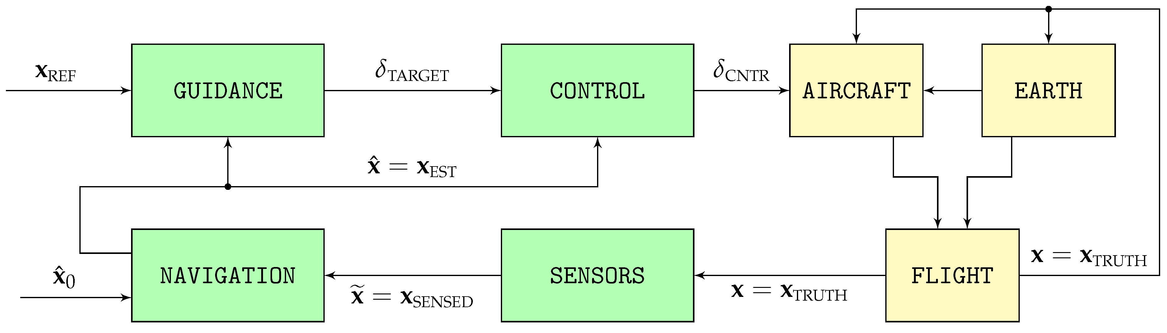
To evaluate the performance of the proposed visual navigation algorithms, this article relies on Monte Carlo simulations consisting of 100 runs each of two different scenarios based on the high fidelity stochastic flight simulator graphically depicted in Figure 4. Described in detail in [15] and with its open source C++ implementation available in [16], the simulator models the flight in varying weather and turbulent conditions of a fixed wing piston engine autonomous UAV.

The simulator consists of two distinct processes. The first, represented by the yellow blocks on the right of Figure 4, models the physics of flight and the interaction between the aircraft and its surroundings that results in the real aircraft trajectory ${\displaystyle \mathbf{x}={\mathbf{x}}_{\mathrm{TRUTH}}}$; the second, represented by the green blocks on the left, contains the aircraft systems in charge of ensuring that the resulting trajectory adheres as much as possible to the mission objectives. It includes the different sensors whose output comprise the sensed trajectory ${\displaystyle \tilde{\mathbf{x}}={\mathbf{x}}_{\mathrm{SENSED}}}$, the navigation system in charge of filtering it to obtain the estimated trajectory ${\displaystyle \widehat{\mathbf{x}}={\mathbf{x}}_{\mathrm{EST}}}$, the guidance system that converts the reference objectives ${\displaystyle {\mathbf{x}}_{\mathrm{REF}}}$ into the control targets ${\displaystyle {\mathbf{\delta }}_{\mathrm{TARGET}}}$, and the control system that adjusts the position of the throttle and aerodynamic control surfaces ${\displaystyle {\mathbf{\delta }}_{\mathrm{CNTR}}}$ so the estimated trajectory ${\displaystyle \widehat{\mathbf{x}}={\mathbf{x}}_{\mathrm{EST}}}$ is as close as possible to the reference objectives ${\displaystyle {\mathbf{x}}_{\mathrm{REF}}}$.

Table 3. Working frequencies of the different systems and trajectory representations.

Discrete Time	Frequency	Period	Variables	Systems
${\displaystyle {\mathrm{t}}_{\mathrm{t}}=\mathrm{t}·\mathit{\Delta }{\mathrm{t}}_{\mathrm{TRUTH}}}$	${\displaystyle 500\mathrm{Hz}}$	${\displaystyle 0.002\mathrm{s}}$	${\displaystyle \mathbf{x}={\mathbf{x}}_{\mathrm{TRUTH}}}$	Flight physics
${\displaystyle {\mathrm{t}}_{\mathrm{s}}=\mathrm{s}·\mathit{\Delta }{\mathrm{t}}_{\mathrm{SENSED}}}$	${\displaystyle 100\mathrm{Hz}}$	${\displaystyle 0.01\mathrm{s}}$	${\displaystyle \tilde{\mathbf{x}}={\mathbf{x}}_{\mathrm{SENSED}}}$	Sensors
${\displaystyle {\mathrm{t}}_{\mathrm{n}}=\mathrm{n}·\mathit{\Delta }{\mathrm{t}}_{\mathrm{EST}}}$	${\displaystyle 100\mathrm{Hz}}$	${\displaystyle 0.01\mathrm{s}}$	${\displaystyle \widehat{\mathbf{x}}={\mathbf{x}}_{\mathrm{EST}}}$	Inertial navigation
${\displaystyle {\mathrm{t}}_{\mathrm{c}}=\mathrm{c}·\mathit{\Delta }{\mathrm{t}}_{\mathrm{CNTR}}}$	${\displaystyle 50\mathrm{Hz}}$	${\displaystyle 0.02\mathrm{s}}$	${\displaystyle {\mathbf{\delta }}_{\mathrm{TARGET}},{\mathbf{\delta }}_{\mathrm{CNTR}}}$	Guidance and control
${\displaystyle {\mathrm{t}}_{\mathrm{i}}=\mathrm{i}·\mathit{\Delta }{\mathrm{t}}_{\mathrm{IMG}}}$	${\displaystyle 10\mathrm{Hz}}$	${\displaystyle 0.1\mathrm{s}}$	${\displaystyle \stackrel{\circ }{\mathbf{x}}={\mathbf{x}}_{\mathrm{IMG}}}$	Visual navigation and camera

provides the working frequencies employed for the different trajectories shown in Figure 4, Figure 5, Figure 6 and Figure 7.

All components of the flight simulator have been modeled with as few simplifications as possible to increase the realism of the results, as explained in [15,17]. With the exception of the aircraft performances and its control system, which are deterministic, all other simulator components are treated as stochastic and hence vary from one execution to the next, enhancing the significance of the Monte Carlo simulation results.

6.1. Camera

The flight simulator has the capability, when provided with the camera pose (the camera is positioned facing down and rigidly attached to the aircraft structure) with respect to the Earth at equally spaced time intervals, of generating images that resemble the view of the Earth surface that the camera would record if located at that particular pose. To do so, it relies on the Earth Viewer library, a modification to osgEarth [18] (which, in turn, relies on OpenSceneGraph [19]) capable of generating realistic Earth images as long as the camera height over the terrain is significantly higher than the vertical relief present in the image. A more detailed explanation of the image generation process is provided in [17].

It is assumed that the shutter speed is sufficiently high that all images are equally sharp, and that the image generation process is instantaneous. In addition, the camera ISO setting remains constant during the flight, and all generated images are noise free. The simulation also assumes that the visible spectrum radiation reaching all patches of the Earth surface remains constant, and the terrain is considered Lambertian [20], so its appearance at any given time does not vary with the viewing direction. The combined use of these assumptions implies that a given terrain object is represented with the same luminosity in all images, even as its relative pose (position and attitude) with respect to the camera varies. Geometrically, the simulation adopts a perspective projection or pinhole camera model [20], which, in addition, is perfectly calibrated and hence shows no distortion. The camera has a focal length of ${\displaystyle 19\mathrm{mm}}$ and a sensor with 768 by 1024 pixels.

6.2. Scenarios

Most visual inertial odometry (VIO) packages discussed in Appendix B include in their release articles an evaluation when applied to the EuRoC Micro Air Vehicle (MAV) datasets [21], and so do independent articles, such as [22]. These datasets contain perfectly synchronized stereo images, Inertial Measurement Unit (IMU) measurements, and ground truth readings obtained with a laser, for 11 different indoor trajectories flown with a MAV, each with a duration in the order of two minutes and a total distance in the order of ${\displaystyle 100\mathrm{m}}$. This fact by itself indicates that the target application of exiting VIO implementations differs significantly from the main focus of this article, which is the long term flight of a fixed wing UAV in GNSS-Denied conditions, as there may exist accumulating errors that are completely non discernible after such short periods of time, but that grow non-linearly and have the capability of inducing significant pose errors when the aircraft remains aloft for long periods of time.

The algorithms introduced in this article are hence tested through simulation under two different scenarios designed to analyze the consequences of losing the GNSS signals for long periods of time. Although a short summary is included below, detailed descriptions of the mission, weather, and wind field employed in each scenario can be found in [15]. Most parameters comprising the scenario are defined stochastically, resulting in different values for every execution. Note that all results shown in Section 7 and Section 8 are based on Monte Carlo simulations comprising 100 runs of each scenario, testing the sensitivity of the proposed navigation algorithms to a wide variety of values in the parameters.

• Scenario #1 has been defined with the objective of adequately representing the challenges faced by an autonomous fixed wing UAV that suddenly cannot rely on GNSS and hence changes course to reach a predefined recovery location situated at approximately one hour of flight time. In the process, in addition to executing an altitude and airspeed adjustment, the autonomous aircraft faces significant weather and wind field changes that make its GNSS-Denied navigation even more challenging.
  With respect to the mission, the stochastic parameters include the initial airspeed, pressure altitude, and bearing (${\displaystyle {\mathrm{v}}_{\mathrm{TAS},\mathrm{INI}},{\mathrm{H}}_{\mathrm{P},\mathrm{INI}},{\varnothing }_{\mathrm{INI}}}$), their final values (${\displaystyle {\mathrm{v}}_{\mathrm{TAS},\mathrm{END}},{\mathrm{H}}_{\mathrm{P},\mathrm{END}},{\varnothing }_{\mathrm{END}}}$), and the time at which each of the three maneuvers is initiated (turns are executed with a bank angle of ${\displaystyle {\xi }_{\mathrm{TURN}}=\pm 10{}^{\circ }}$, altitude changes employ an aerodynamic path angle of ${\displaystyle {\gamma }_{\mathrm{TAS},\mathrm{CLIMB}}=\pm 2{}^{\circ }}$, and airspeed modifications are automatically executed by the control system as set-point changes). The scenario lasts for ${\displaystyle {\mathrm{t}}_{\mathrm{END}}=3800\mathrm{s}}$, while the GNSS signals are lost at ${\displaystyle {\mathrm{t}}_{\mathrm{GNSS}}=100\mathrm{s}}$.
  The wind field is also defined stochastically, as its two parameters (speed and bearing) are constant both at the beginning (${\displaystyle {\mathrm{v}}_{\mathrm{WIND},\mathrm{INI}},{\varnothing }_{\mathrm{WIND},\mathrm{INI}}}$) and conclusion (${\displaystyle {\mathrm{v}}_{\mathrm{WIND},\mathrm{END}},{\varnothing }_{\mathrm{WIND},\mathrm{END}}}$) of the scenario, with a linear transition in between. The specific times at which the wind change starts and concludes also vary stochastically among the different simulation runs. As described in [15], the turbulence remains strong throughout the whole scenario, but its specific values also vary stochastically from one execution to the next.
  A similar linear transition occurs with the temperature and pressure offsets that define the atmospheric properties [23], as they are constant both at the start (${\displaystyle \mathit{\Delta }{\mathrm{T}}_{\mathrm{INI}},\mathit{\Delta }{\mathrm{p}}_{\mathrm{INI}}}$) and end (${\displaystyle \mathit{\Delta }{\mathrm{T}}_{\mathrm{END}},\mathit{\Delta }{\mathrm{p}}_{\mathrm{END}}}$) of the flight. In contrast with the wind field, the specific times at which the two transitions start and conclude are not only stochastic but also different from each other.
• Scenario #2 represents the challenges involved in continuing with the original mission upon the loss of the GNSS signals, executing a series of continuous turn maneuvers over a relatively short period of time with no atmospheric or wind variations. As in scenario ${\displaystyle \#1}$, the GNSS signals are lost at ${\displaystyle {\mathrm{t}}_{\mathrm{GNSS}}=100\mathrm{s}}$, but the scenario duration is shorter (${\displaystyle {\mathrm{t}}_{\mathrm{END}}=500\mathrm{s}}$). The initial airspeed and pressure altitude (${\displaystyle {\mathrm{v}}_{\mathrm{TAS},\mathrm{INI}},{\mathrm{H}}_{\mathrm{P},\mathrm{INI}}}$) are defined stochastically and do not change throughout the whole scenario; the bearing however changes a total of eight times between its initial and final values, with all intermediate bearing values, as well as the time for each turn varying stochastically from one execution to the next. Although the same turbulence is employed as in scenario ${\displaystyle \#1}$, the wind and atmospheric parameters (${\displaystyle {\mathrm{v}}_{\mathrm{WIND},\mathrm{INI}},{\varnothing }_{\mathrm{WIND},\mathrm{INI}},\mathit{\Delta }{\mathrm{T}}_{\mathrm{INI}},\mathit{\Delta }{\mathrm{p}}_{\mathrm{INI}}}$) remain constant throughout scenario ${\displaystyle \#2}$.

7. Results: Navigation System Error in GNSS-Denied Conditions

This section presents the results obtained with the proposed Inertially Assisted Visual Navigation System or IA-VNS (comprised by SVO, as described in Appendix C and Section 4, together with the proposed modifications described in Section 5) when executing Monte Carlo simulations of the two GNSS-Denied scenarios over the MX terrain type (Section 8 defines various terrain types, and then analyzes their influence on the simulation results), each consisting of 100 executions. They are compared with the results obtained with the standalone Visual Navigation System or VNS that relies on the baseline SVO pipeline (Appendix C and Section 4), and with those of the Inertial Navigation System or INS described in [6].

Table 4. Aggregated MX final body attitude INSE, VNSE, and IA-VNSE (100 runs). The most important metrics appear in bold.

	NSE				VNSE				IA-VNSE
${\displaystyle \left[{}^{\mathbf{\circ }}\right]}$	${\displaystyle \mathit{\Delta }\widehat{\mathbf{\psi }}}$	${\displaystyle \mathit{\Delta }\widehat{\mathbf{\theta }}}$	${\displaystyle \mathit{\Delta }\widehat{\mathbf{\xi }}}$	${\displaystyle \mathbf{\parallel }\mathit{\Delta }{\widehat{\mathbf{r}}}_{\mathbf{NB}}^{\mathbf{B}}\mathbf{\parallel }}$	${\displaystyle \mathit{\Delta }\stackrel{\mathbf{\circ }}{\mathbf{\psi }}}$	${\displaystyle \mathit{\Delta }\stackrel{\mathbf{\circ }}{\mathbf{\theta }}}$	${\displaystyle \mathit{\Delta }\stackrel{\mathbf{\circ }}{\mathbf{\xi }}}$	${\displaystyle \mathbf{\parallel }\mathit{\Delta }{\stackrel{\mathbf{\circ }}{\mathbf{r}}}_{\mathbf{NB}}^{\mathbf{B}}\mathbf{\parallel }}$	${\displaystyle \mathit{\Delta }\stackrel{\mathbf{\circ }}{\mathbf{\psi }}}$	${\displaystyle \mathit{\Delta }\stackrel{\mathbf{\circ }}{\mathbf{\theta }}}$	${\displaystyle \mathit{\Delta }\stackrel{\mathbf{\circ }}{\mathbf{\xi }}}$	${\displaystyle \mathbf{\parallel }\mathit{\Delta }{\stackrel{\mathbf{\circ }}{\mathbf{r}}}_{\mathbf{NB}}^{\mathbf{B}}\mathbf{\parallel }}$
Scenario #1 MX ${\displaystyle \left({\mathrm{t}}_{\mathrm{END}}\right)}$
mean	+0.03	${\displaystyle -}$0.03	${\displaystyle -}$0.00	0.158	+0.03	+0.08	+0.00	0.296	+0.03	${\displaystyle -}$0.01	${\displaystyle -}$0.03	0.218
std	0.18	0.05	0.06	0.114	0.13	0.23	0.21	0.158	0.11	0.16	0.14	0.103
max	${\displaystyle -}$0.61	${\displaystyle -}$0.27	${\displaystyle -}$0.23	0.611	+0.63	+0.74	+0.78	0.791	+0.55	${\displaystyle -}$0.37	${\displaystyle -}$0.51	0.606
Scenario #2 MX ${\displaystyle \left({\mathrm{t}}_{\mathrm{END}}\right)}$
mean	${\displaystyle -}$0.02	+0.01	+0.00	0.128	+0.02	${\displaystyle -}$0.02	+0.00	0.253	+0.02	${\displaystyle -}$0.00	+0.01	0.221
std	0.13	0.05	0.05	0.078	0.08	0.21	0.20	0.161	0.08	0.16	0.19	0.137
max	+0.33	${\displaystyle -}$0.15	+0.15	0.369	+0.22	${\displaystyle -}$0.65	${\displaystyle -}$0.73	0.730	+0.24	+0.62	+0.74	0.788

,

Table 5. Aggregated MX final vertical position INSE, VNSE, and IA-VNSE (100 runs). The most important metrics appear in bold.

Scenario MX ${\displaystyle \left({\mathbf{t}}_{\mathbf{END}}\right)}$		INSE	VNSE	IA-VNSE
	${\displaystyle \left[\mathbf{m}\right]}$	${\displaystyle \mathit{\Delta }\widehat{\mathbf{h}}}$	${\displaystyle \mathit{\Delta }\stackrel{\mathbf{\circ }}{\mathbf{h}}}$	${\displaystyle \mathit{\Delta }\stackrel{\mathbf{\circ }}{\mathbf{h}}}$
#1	mean	${\displaystyle -}$4.18	+82.91	+22.86
	std	25.78	287.58	49.17
	max	${\displaystyle -}$70.49	+838.32	+175.76
#2	mean	+0.76	+3.45	+3.59
	std	7.55	20.56	13.01
	max	${\displaystyle -}$19.86	+72.69	+71.64

and

Table 6. Aggregated MX final horizontal position INSE, VNSE, and IA-VNSE (100 runs). The most important metrics appear in bold.

Scenario MX ${\displaystyle \left({\mathbf{t}}_{\mathbf{END}}\right)}$			INSE		VNSE		IA-VNSE
		Distance	${\displaystyle \mathit{\Delta }{\widehat{\mathbf{x}}}_{\mathbf{HOR}}}$		${\displaystyle \mathit{\Delta }{\stackrel{\mathbf{\circ }}{\mathbf{x}}}_{\mathbf{HOR}}}$		${\displaystyle \mathit{\Delta }{\stackrel{\mathbf{\circ }}{\mathbf{x}}}_{\mathbf{HOR}}}$
		${\displaystyle \left[\mathrm{m}\right]}$	${\displaystyle \left[\mathrm{m}\right]}$	${\displaystyle \left[\%\right]}$	${\displaystyle \left[\mathrm{m}\right]}$	${\displaystyle \left[\%\right]}$	${\displaystyle \left[\mathrm{m}\right]}$	${\displaystyle \left[\%\right]}$
${\displaystyle \#1}$	mean	107,873	7276	7.10	4179	3.82	488	0.46
	std	19,756	4880	5.69	3308	2.73	350	0.31
	max	172,842	25,288	32.38	21,924	14.22	1957	1.48
${\displaystyle \#2}$	mean	14,198	216	1.52	251	1.77	33	0.23
	std	1176	119	0.86	210	1.48	26	0.18
	max	18,253	586	4.38	954	7.08	130	0.98

contain the navigation system error or NSE (difference between the real or true states ${\displaystyle \mathbf{x}}$ and their inertial ${\displaystyle \widehat{\mathbf{x}}}$ or visual ${\displaystyle \stackrel{\circ }{\mathbf{x}}}$ estimations) incurred by the various navigation systems (and accordingly denoted as INSE, VNSE, and IA-VNSE) at the conclusion of the two GNSS-Denied scenarios, represented by the mean, standard deviation, and maximum value of the estimation errors. In addition, the figures shown in this section depict the variation with time of the NSE mean (solid line) and standard deviation (dashed lines) for the 100 executions. The following remarks are necessary:

• The results obtained with the INS under the same two GNSS-Denied scenarios are described in detail in [6], a previous article by the same authors. It proves that it is possible to take advantage of sensors already present onboard fixed wing aircraft (accelerometers, gyroscopes, magnetometers, Pitot tube, air vanes, thermometer, and barometer), the particularities of fixed wing flight, and the atmospheric and wind estimations that can be obtained before the GNSS signals are lost, to develop an EKF (Extended Kalman Filter)-based INS that results in bounded (no drift) estimations for attitude (ensuring that the aircraft can remain aloft in GNSS-Denied conditions for as long as there is fuel available), altitude (the estimation error depends on the change in atmospheric pressure offset ${\displaystyle \mathit{\Delta }\mathrm{p}}$ [23] from its value at the time the GNSS signals are lost, which is bounded by atmospheric physics), and ground velocity (the estimation error depends on the change in wind velocity from its value at the time the GNSS signals are lost, which is bounded by atmospheric physics), as well as an unavoidable drift in horizontal position caused by integrating the ground velocity without absolute observations. Note that of the six ${\displaystyle \mathbb{SE}\left(3\right)}$ degrees of freedom or the aircraft pose (three for attitude, two for horizontal position, one for altitude), the INS is hence capable of successfully estimating four of them in GNSS-Denied conditions. 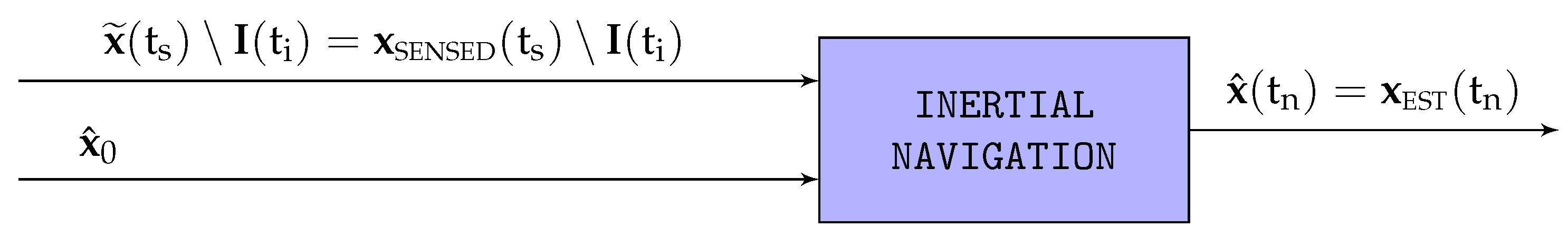Figure 5 graphically depicts that the INS inputs include all sensor measurements ${\displaystyle \tilde{\mathbf{x}}={\mathbf{x}}_{\mathrm{SENSED}}}$ with the exception of the camera images ${\displaystyle \mathbf{I}}$.

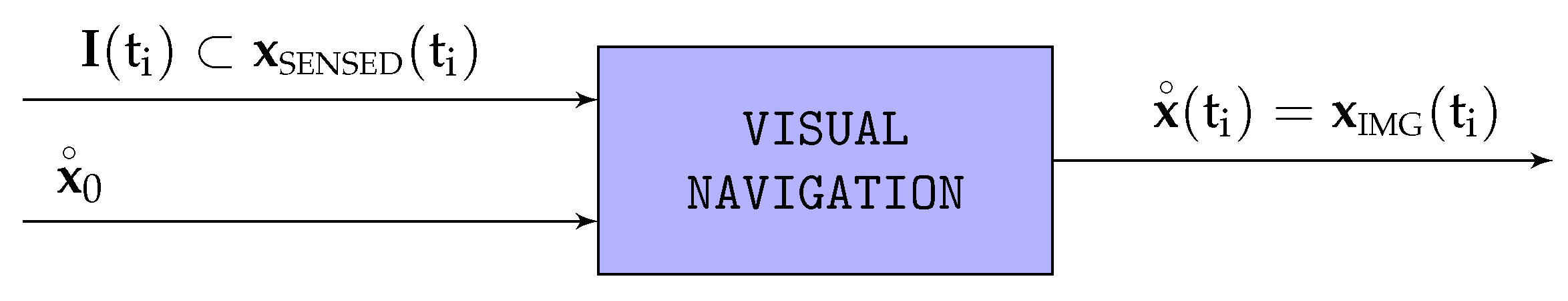
• Visual navigation systems (either VNS or IA-VNS) are only necessary to reduce the estimation error in the two remaining degrees of freedom (the horizontal position). Although both of them estimate the complete six dimensional aircraft pose, their attitude and altitude estimations shall only be understood as a means to provide an accurate horizontal position estimation, which represents their sole objective. 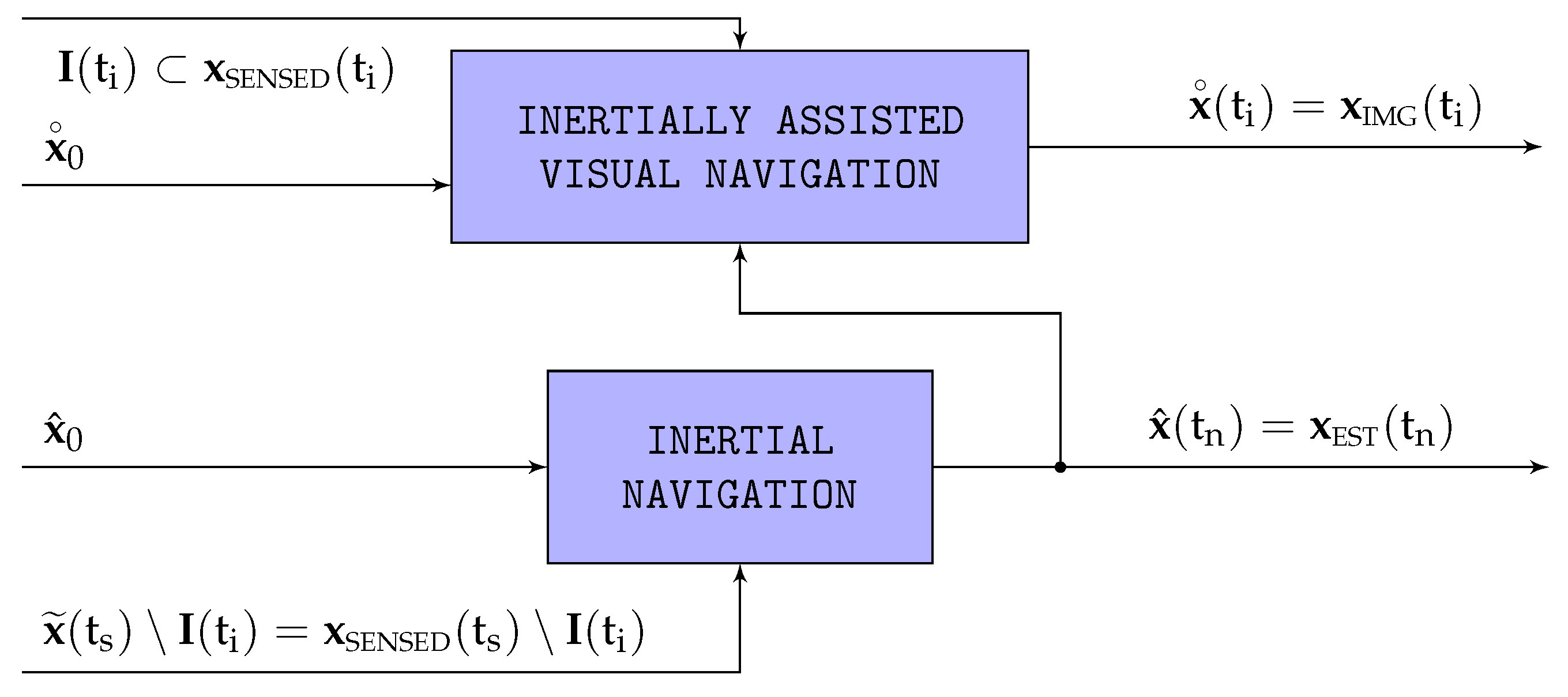Figure 6 shows that the VNS relies exclusively on the images ${\displaystyle \mathbf{I}}$ without the use of any other sensors; on the other hand, the IA-VNS represented in Figure 7 complements the images with the ${\displaystyle \widehat{\mathbf{x}}={\mathbf{x}}_{\mathrm{EST}}}$ outputs of the INS.

• As it does not rely on absolute references, visual navigation slowly accumulates error (drifts) not only in horizontal position, but also in attitude and altitude. The main focus of this article is on how the addition of INS based priors enables the IA-VNS to reduce the drift in all six dimensions, with the resulting horizontal position IA-VNSE being just a fraction of the INSE. The attitude and altitude IA-VNSEs, although improved when compared to the VNSEs, are qualitatively inferior to the driftless INSEs, but note that their purpose is just to enable better horizontal position IA-VNS estimations, not to replace the attitude and altitude INS outputs.

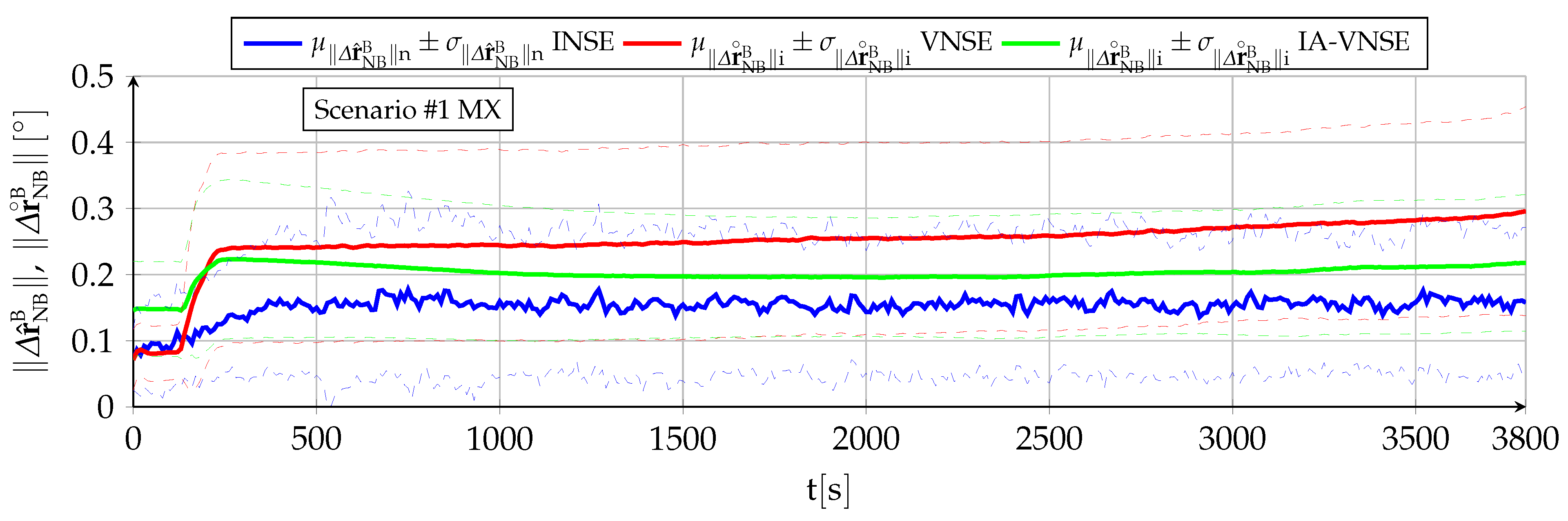
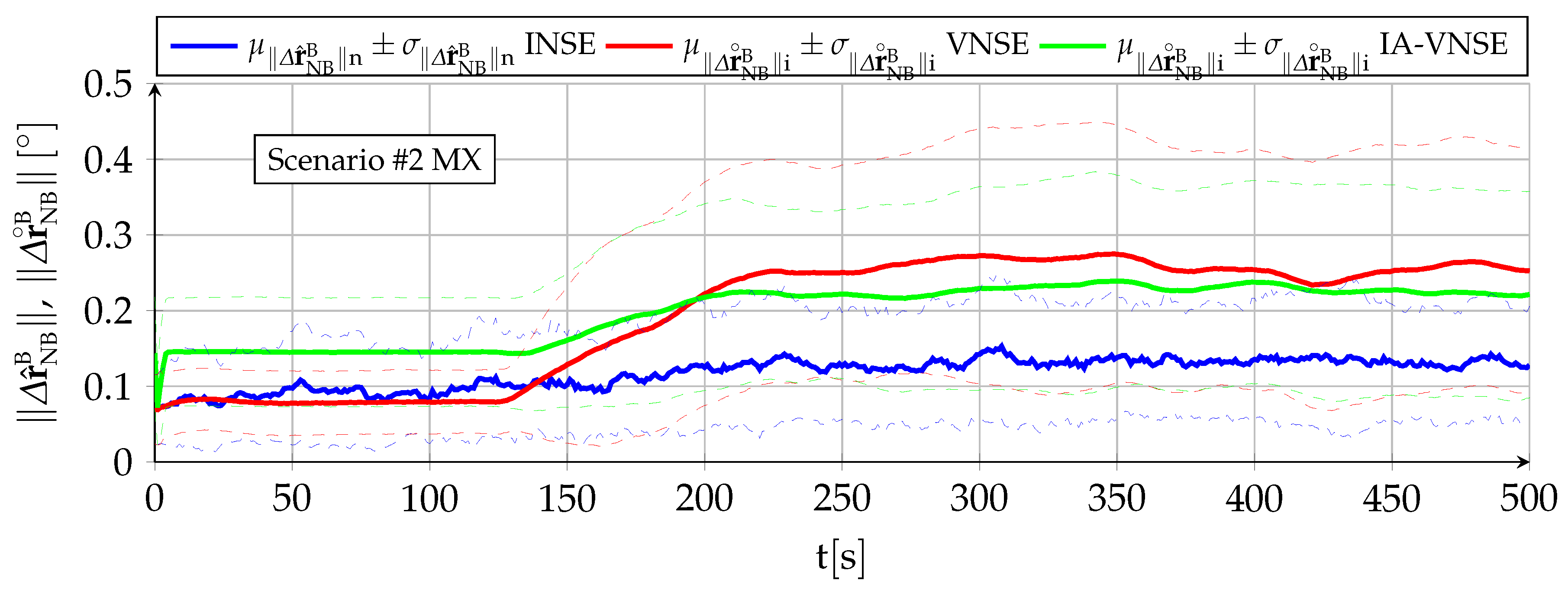
7.1. Body Attitude Estimation

Table 4 shows the NSE at the conclusion of both scenarios for the three Euler angles representing the body attitude (yaw ${\displaystyle \psi }$, pitch ${\displaystyle \theta }$, roll ${\displaystyle \xi }$), as well as the norm of the rotation vector between the real body attitude ${\displaystyle {\mathbf{q}}_{\mathrm{NB}}}$ and its estimations, ${\displaystyle {\widehat{\mathbf{q}}}_{\mathrm{NB}}}$ by the INS and ${\displaystyle {\stackrel{\circ }{\mathbf{q}}}_{\mathrm{NB}}}$ by the VNS or IA-VNS. The yaw angle estimation errors respond to ${\displaystyle \mathit{\Delta }\widehat{\psi }=\widehat{\psi }-\psi }$ and ${\displaystyle \mathit{\Delta }\stackrel{\circ }{\psi }=\stackrel{\circ }{\psi }-\psi }$, respectively; those for the body pitch and roll angles are defined accordingly. In the case of the rotation vector, the errors can be formally written as ${\displaystyle \parallel \mathit{\Delta }{\widehat{\mathbf{r}}}_{\mathrm{NB}}^{\mathrm{B}}\parallel =\parallel {\widehat{\mathbf{q}}}_{\mathrm{NB}}\ominus {\mathbf{q}}_{\mathrm{NB}}\parallel }$ or ${\displaystyle \parallel \mathit{\Delta }{\stackrel{\circ }{\mathbf{r}}}_{\mathrm{NB}}^{\mathrm{B}}\parallel =\parallel {\stackrel{\circ }{\mathbf{q}}}_{\mathrm{NB}}\ominus {\mathbf{q}}_{\mathrm{NB}}\parallel }$ [1], where ${\displaystyle \ominus }$ represents the ${\displaystyle \mathbb{SO}\left(3\right)}$ minus operator. 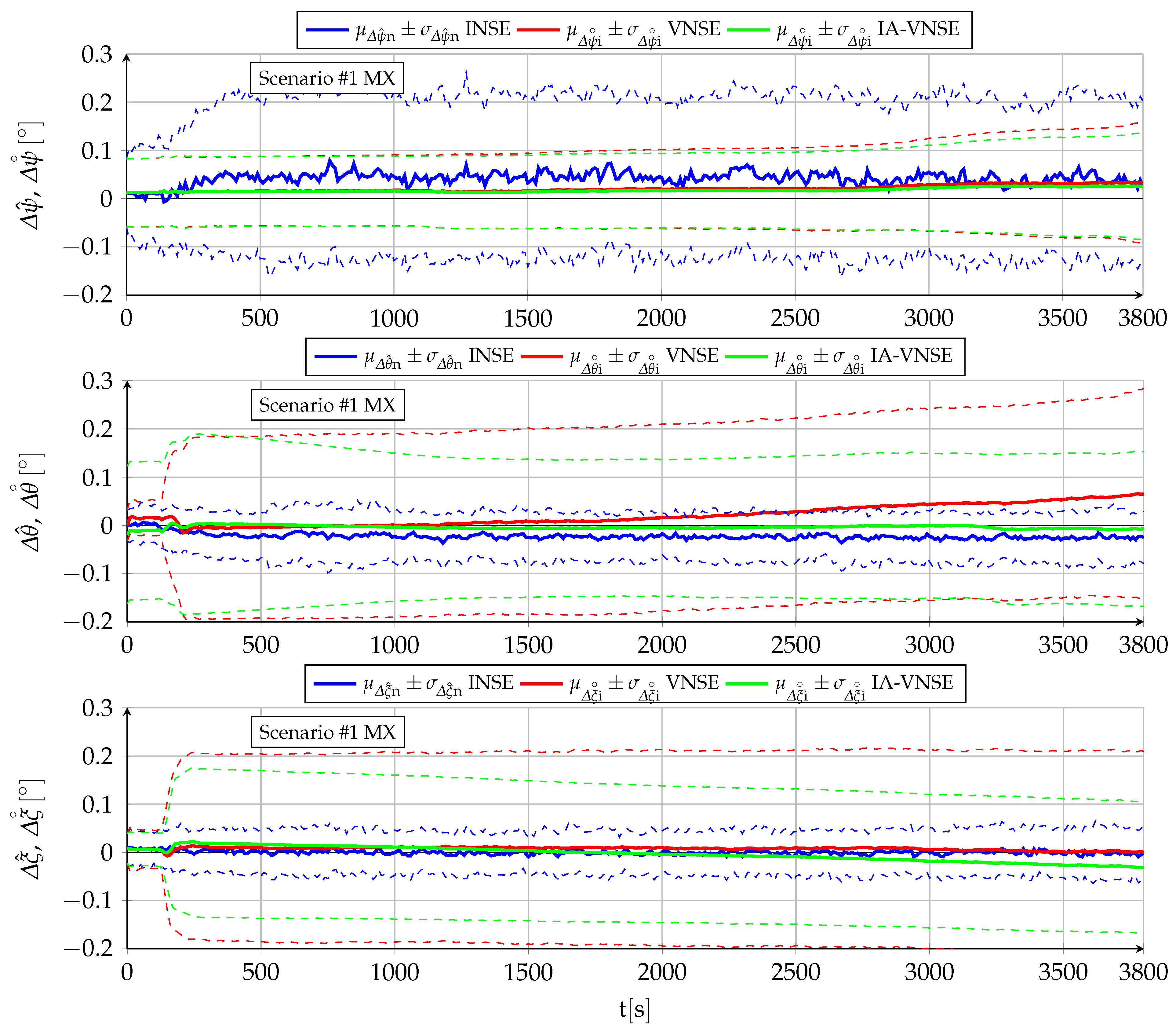In addition, Figure 8 and Figure 9 depict the variation with time of the body attitude NSE for both scenarios, while Figure 10 shows those of each individual Euler angle for scenario ${\displaystyle \#1}$ exclusively.

• After a short transition period following the introduction of GNSS-Denied conditions at ${\displaystyle {\mathrm{t}}_{\mathrm{GNSS}}=100\mathrm{s}}$, the body attitude inertial navigation system error or INSE (blue lines) does not experience any drift with time in either scenario, and is bounded by the quality of the onboard sensors and the inertial navigation algorithms [6].

• With respect to the visual navigation system error or VNSE (red lines), most of the scenario ${\displaystyle \#1}$ error is incurred during the turn maneuver at the beginning of the scenario (refer to ${\displaystyle {\mathrm{t}}_{\mathrm{TURN}}}$ within [15]), with only a slow accumulation during the rest of the trajectory, composed by a long straight flight with punctual changes in altitude and speed. Additional error growth would certainly accumulate if more turns were to occur, although this is not tested in the simulation. This statement seems to contradict the results obtained with scenario ${\displaystyle \#2}$, in which the error grows with the initial turns but then stabilizes during the rest of the scenario, even though the aircraft is executing continuous turn maneuvers. This lack of error growth occurs because the scenario ${\displaystyle \#2}$ trajectories are so twisted (refer to [15]) that terrain zones previously mapped reappear in the camera field of view during the consecutive turns, and are hence employed by the pose optimization phase as absolute references, resulting in a much better attitude estimation than what would occur under more spaced turns. A more detailed analysis (not shown in the figures) shows that the estimation error does not occur during the whole duration of the turns, but only during the roll-in and final roll-out maneuvers, where the optical flow is highest and hence more difficult to track by SVO (for the two evaluated scenarios, the optical flow during the roll-in and roll-out maneuvers is significantly higher than that induced by straight flight, pull-up, and push-down maneuvers, and even the turning maneuvers themselves once the bank angle is no longer changing).

• The inertially assisted VNSE or IA-VNSE results (green lines) show that the introduction of priors in Section 5 works as intended and there exists a clear benefit for the use of an IA-VNS when compared to the standalone VNS described in Appendix C. In spite of IA-VNSE values at the beginning of both scenarios that are nearly double those of the VNSE (refer to Figure 8 and Figure 9), caused by the initial pitch adjustment required to improve the fit between the homography output and the inertial estimations (Section 5.4), the balance between both errors quickly flips as soon as the aircraft starts maneuvering, resulting in body attitude IA-VNSE values significantly lower than those of the VNSE for the remaining part of both scenarios. This improvement is more significant in the case of scenario ${\displaystyle \#1}$, as the prior based pose optimization is by design a slow adjustment that requires significant time to slowly correct attitude and altitude deviations between the visual and inertial estimations.

Qualitatively, the biggest difference between the three estimations resides in the nature of the errors. While the attitude INSE is bounded, drift is present in both the VNS and IA-VNS estimations. The drift resulting from the Monte Carlo simulations may be small, and so is the attitude estimation error ${\displaystyle \parallel \mathit{\Delta }{\stackrel{\circ }{\mathbf{r}}}_{\mathrm{NB}}^{\mathrm{B}}\parallel }$, but more challenging conditions with more drastic maneuvers and a less idealized image generation process than that described in Section 6 may generate additional drift.

Focusing now on the quantitative results shown in Table 4, aggregated errors for each individual Euler angle are always unbiased and zero mean for each of the three estimations (INS, VNS, IA-VNS), as the means tend to zero as the number of runs grows, and are much smaller than both the standard deviations and the maximum values. With respect to the attitude error ${\displaystyle \parallel \mathit{\Delta }{\widehat{\mathbf{r}}}_{\mathrm{NB}}^{\mathrm{B}}\parallel }$ and ${\displaystyle \parallel \mathit{\Delta }{\stackrel{\circ }{\mathbf{r}}}_{\mathrm{NB}}^{\mathrm{B}}\parallel }$, their aggregated means are not zero (they are norms), but are nevertheless quite repetitive in all three cases, as the mean is always significantly higher than the standard deviation, while the maximum values only represent a small multiple of the means. It is interesting to point out that while in the case of the INSE the contribution of the yaw error is significantly higher than that of the pitch and roll errors, the opposite occurs for both the VNSE and the IA-VNSE. This makes sense as the the gravity direction is employed by the INS as a reference from where the estimated pitch and roll angles can not deviate, but slow changes in yaw generate larger optical flow variations than those caused by pitch and roll variations.

These results prove that the algorithms proposed in Section 5 succeed when employing the inertial pitch and bank angles (${\displaystyle \widehat{\theta }}$, ${\displaystyle \widehat{\xi }}$), whose errors are bounded, to limit the drift of their visual counterparts (${\displaystyle \stackrel{\circ }{\theta }}$, ${\displaystyle \stackrel{\circ }{\xi }}$), as ${\displaystyle {\sigma }_{\mathrm{END}\stackrel{\circ }{\theta }}}$ and ${\displaystyle {\sigma }_{\mathrm{END}\stackrel{\circ }{\xi }}}$ are significantly lower for the IA-VNS than for the VNS (as the individual Euler angle metrics are unbiased or zero mean, the benefits of the proposed approach are reflected in the variation of the remaining metrics, this is, the standard deviation and the maximum value). Remarkably, this is achieved with no degradation in the body yaw angle, as ${\displaystyle {\sigma }_{\mathrm{END}\stackrel{\circ }{\psi }}}$ remains stable. Note that adjusting the output of certain variables in a minimization algorithm (such as pose optimization) usually results in a degradation in the accuracy of the remaining variables as the solution moves away from the true optimum. In this case, however, the improved fit between the adjusted aircraft pose and the terrain displayed in the images, results in the SVO pipeline also slightly improving its body yaw estimation ${\displaystyle \stackrel{\circ }{\psi }}$. Section 7.3 shows how the benefits of an improved fit between the displayed terrain and the adjusted pose also improve the horizontal position estimation.

In the case of a real life scenario based on a more realistic image generation process than that described in Section 6, the VNS would likely incur in additional body attitude drift than in the simulations. If this were to occur, the IA-VNS pose adjustment algorithms described in Section 5 would react more aggressively to counteract the higher pitch and bank deviations, eliminating most of the extra drift, although it is possible that higher pose adjustment parameters than those listed in Table 2 would be required. The IA-VNS is hence more resilient against high drift values than the VNS.

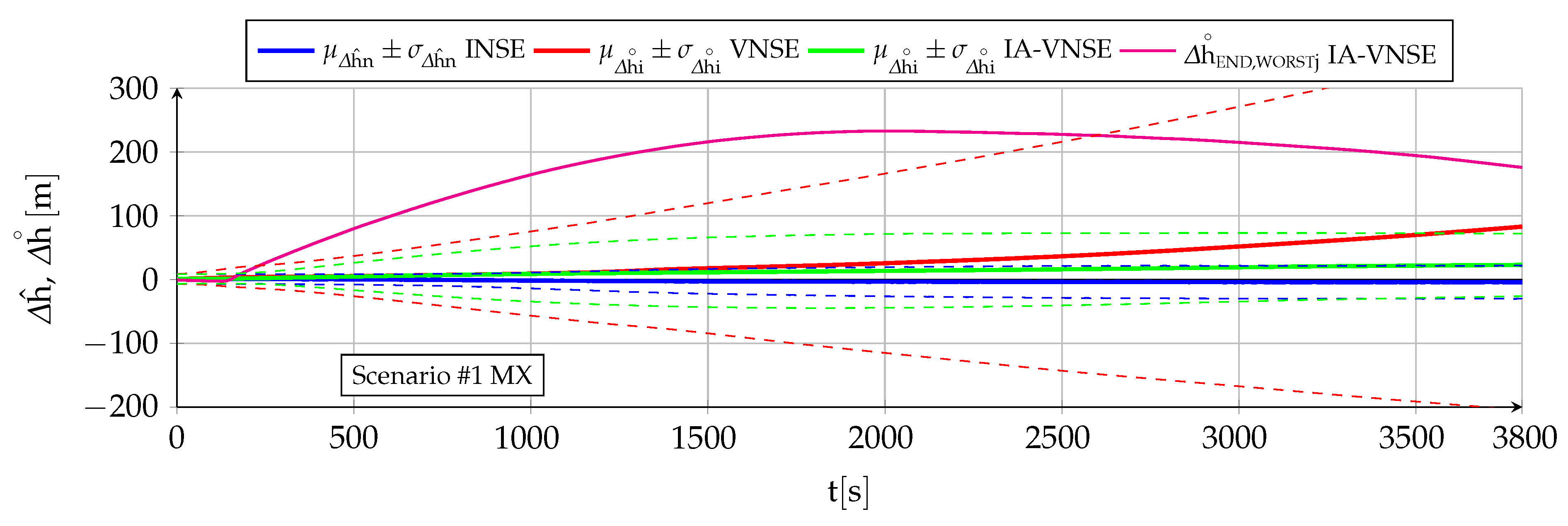
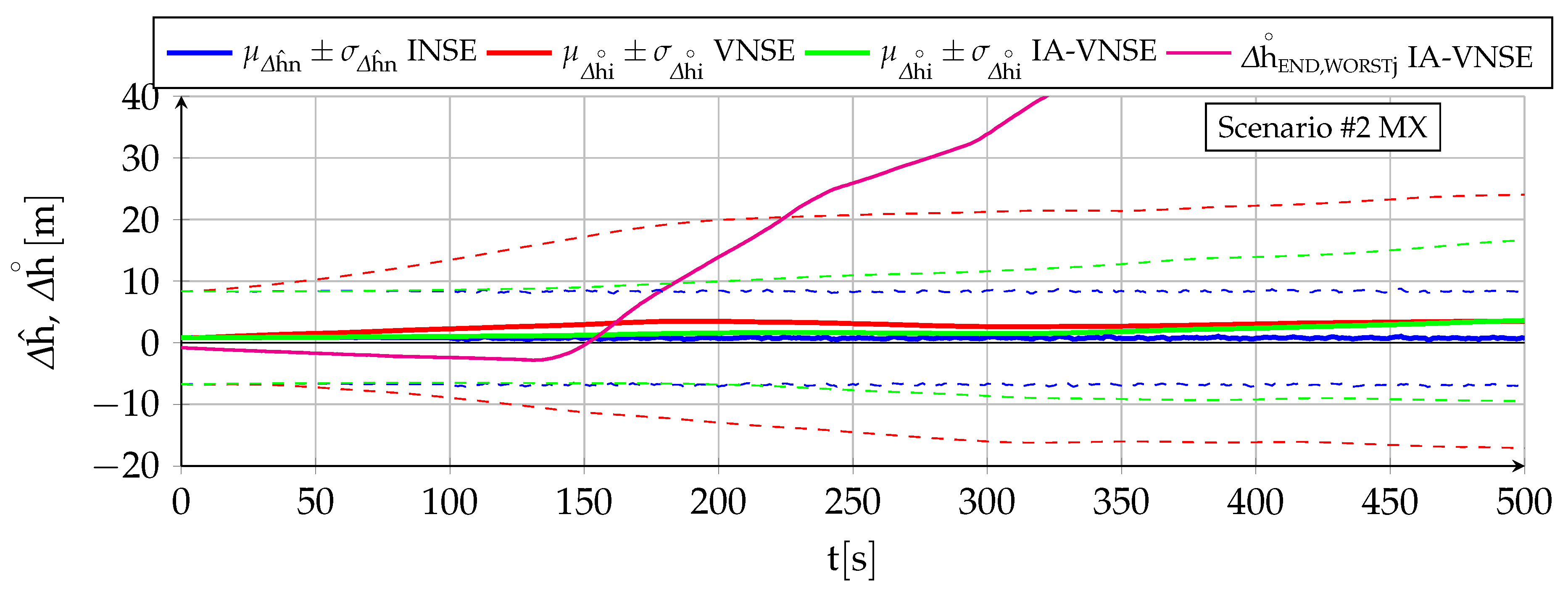
7.2. Vertical Position Estimation

Table 5 contains the vertical position NSE (${\displaystyle \mathit{\Delta }\widehat{\mathrm{h}}=\widehat{\mathrm{h}}-\mathrm{h}}$, ${\displaystyle \mathit{\Delta }\stackrel{\circ }{\mathrm{h}}=\stackrel{\circ }{\mathrm{h}}-\mathrm{h}}$) at the conclusion of both scenarios, which can be considered unbiased or zero mean in all six cases (two scenarios and three estimation methods) as the mean ${\displaystyle {\mu }_{\mathrm{END}\mathrm{h}}}$ is always significantly lower than both the standard deviation ${\displaystyle {\sigma }_{\mathrm{END}\mathrm{h}}}$ or the maximum value ${\displaystyle {\mathbf{\zeta }}_{\mathrm{END}\left|\mathrm{h}\right|}}$. The NSE evolution with time is depicted in Figure 11 and Figure 12, which also include (magenta lines) those Monte Carlo executions that result in the highest IA-VNSEs.

• The geometric altitude INSE (blue lines) is bounded by the change in atmospheric pressure offset since the time the GNSS signals are lost. Refer to [6] for additional information.
• The VNS estimation of the geometric altitude (red lines) is worse than that by the INS both qualitatively and quantitatively, even with the results being optimistic because of the ideal image generation process employed in the simulation. A continuous drift or error growth with time is present, and results in final errors much higher than those obtained with the GNSS-Denied inertial filter. These errors are logically bigger for scenario ${\displaystyle \#1}$ because of its much longer duration.
  A small percentage of this drift can be attributed to the slow accumulation of error inherent to the SVO motion thread algorithms introduced in Appendix C, but most of it results from adding the estimated relative pose between two consecutive images to a pose (that of the previous image) with an attitude that already possesses a small pitch error (refer to the attitude estimation analysis in Section 7.1). Note that even a fraction of a degree deviation in pitch can result in hundreds of meters in vertical error when applied to the total distance flown in scenario ${\displaystyle \#1}$, as SVO can be very precise when estimating pose changes between consecutive images, but lacks any absolute reference to avoid slowly accumulating these errors over time. This fact is precisely the reason why the vertical position VNSE grows more slowly in the second half of scenario ${\displaystyle \#2}$, as shown in Figure 12. As explained in Section 7.1 above, continuous turn maneuvers cause previously mapped terrain points to reappear in the camera field of view, stopping the growth in the attitude error (pitch included), which indirectly has the effect of slowing the growth in altitude estimation error.
• The benefits of introducing priors to limit the differences between the visual and inertial altitude estimations are reflected in the IA-VNSE (green lines). The error reduction is drastic in the case of the scenario ${\displaystyle \#1}$, where its extended duration allows the pose optimization small pitch adjustments to accumulate into significant altitude corrections over time, and less pronounced but nevertheless significant for scenario ${\displaystyle \#2}$, where the VNSE (an hence also the IA-VNSE) results already benefit from previously mapped terrain points reappearing in the aircraft field of view as a result of the continuous maneuvers. It is necessary to remark the amount of the improvement, as the final standard deviation ${\displaystyle {\sigma }_{\mathrm{END}\mathrm{h}}}$ diminishes from ${\displaystyle 287.58}$ to ${\displaystyle 49.17\mathrm{m}}$ for scenario ${\displaystyle \#1}$, and from ${\displaystyle 20.56}$ to ${\displaystyle 13.01\mathrm{m}}$ for scenario ${\displaystyle \#2}$.

The benefits of the prior based pose optimization algorithm can be clearly observed in the case of the scenario ${\displaystyle \#1}$ execution with the worst final altitude estimation error, whose error variation with time is depicted in Figure 11 (magenta line). After a rapid growth in the first third of the scenario following a particularly negative estimation during the initial turn, the altitude error reaches a maximum of ${\displaystyle +233.05\mathrm{m}}$ at ${\displaystyle 2007.5\mathrm{}\mathrm{s}}$. Attitude adjustment has become active long before, lowering the estimated pitch angle to first diminish the growth of the altitude error and then being able to reduce the error itself, reaching a final value of ${\displaystyle +175.76\mathrm{m}}$ at ${\displaystyle {\mathrm{t}}_{\mathrm{END}}}$. As soon as the differences between the visual pitch, bank, or altitude estimations (${\displaystyle \stackrel{\circ }{\theta },\stackrel{\circ }{\xi },\stackrel{\circ }{\mathrm{h}}}$) and their inertial counterparts (${\displaystyle \widehat{\theta },\widehat{\xi },\widehat{\mathrm{h}}}$) exceed certain limits (Section 5), the attitude adjustment comes into play and slowly adjusts the aircraft pitch to prevent the visual altitude from deviating in excess from the inertial one. This behavior not only improves the IA-VNS altitude estimation accuracy when compared to that of the VNS, but also its resilience, as the system actively opposes elevated altitude errors.

Significantly better altitude estimation errors (closer to the inertial ones) could be obtained if more aggressive settings were employed for ${\displaystyle \mathit{\Delta }{\stackrel{\circ }{\theta }}_{1,\mathrm{MAX}}^{\circ \circ }}$ and ${\displaystyle \mathit{\Delta }{\stackrel{\circ }{\theta }}_{2,\mathrm{MAX}}^{\circ \circ }}$ within Table 2, as the selected values are far from the level at which the pose optimization convergence is compromised. This would result in more aggressive adjustments and important accuracy improvements for those cases in which altitude error growth is highest. The settings employed in this article are modest, as the final objective is not to obtain the smallest possible attitude or vertical position IA-VNSE (as they are always bigger than their INSE counterparts), but to limit them to acceptable levels so SVO can build a more accurate terrain map, improving the fit between the multiple terrain 3D points displayed in the images and the estimated aircraft pose. To do so it is mandatory to balance the pitch and bank angle adjustments with the need to stick to solutions close to those that minimize the reprojection error, as explained in Section 5. Higher ${\displaystyle \mathit{\Delta }{\stackrel{\circ }{\theta }}_{1,\mathrm{MAX}}^{\circ \circ }}$ and ${\displaystyle \mathit{\Delta }{\stackrel{\circ }{\theta }}_{2,\mathrm{MAX}}^{\circ \circ }}$ accelerate the adjustments but may decrease the quality of the map. It is expected that a better rendition of the real 3D position of the features detected in the keyframes as they are tracked along successive images will lower the incremental horizontal displacement errors, and, hence, result in a lower horizontal position IA-VNSE, which is the real objective for the introduction of the priors.

The IA-VNS altitude estimation improvements over those of the VNS are not only quantitative. Figure 11 shows no increment in ${\displaystyle {\sigma }_{\stackrel{\circ }{\mathrm{h}}\mathrm{n}}}$ (green lines) in the second half of scenario ${\displaystyle \#1}$ (once on average the deviation has activated the attitude adjustment feature). The altitude estimation by the IA-VNS can hence also be described as bounded and driftless, which represents a qualitative and not only quantitative improvement over that of the VNS. The bounds are obviously bigger for the IA-VNS than for the INS. In the case of scenario ${\displaystyle \#2}$, Figure 12 shows a slow but steady ${\displaystyle {\sigma }_{\stackrel{\circ }{\mathrm{h}}\mathrm{n}}}$ growth with time, but this is only because the error amount on average is not yet significant enough to activate the attitude adjustment feature within pose optimization.

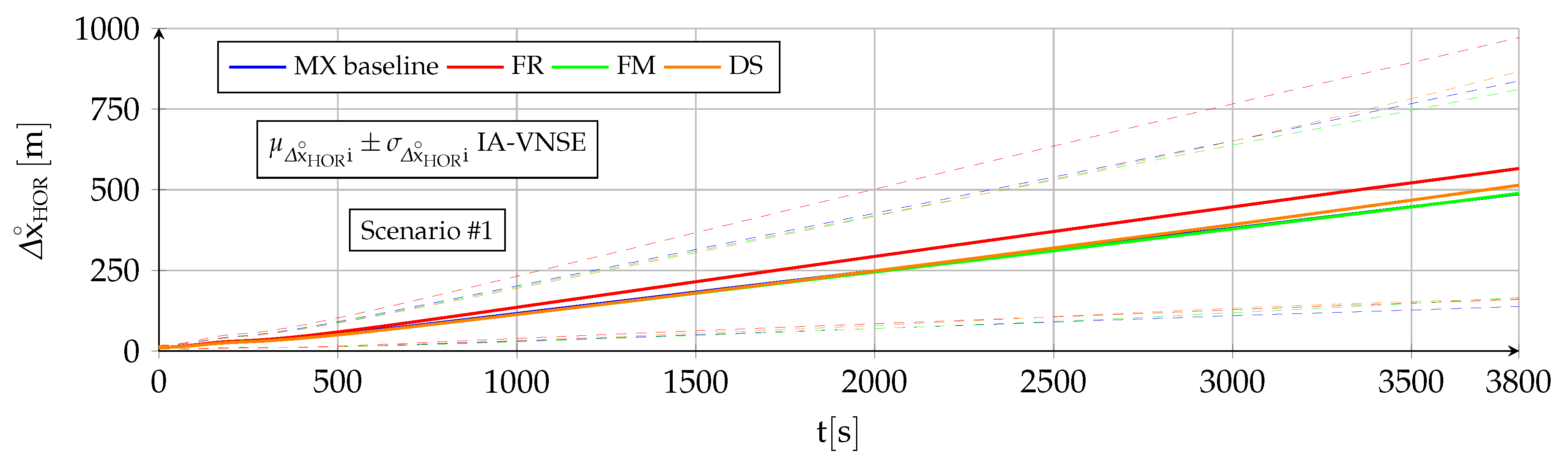
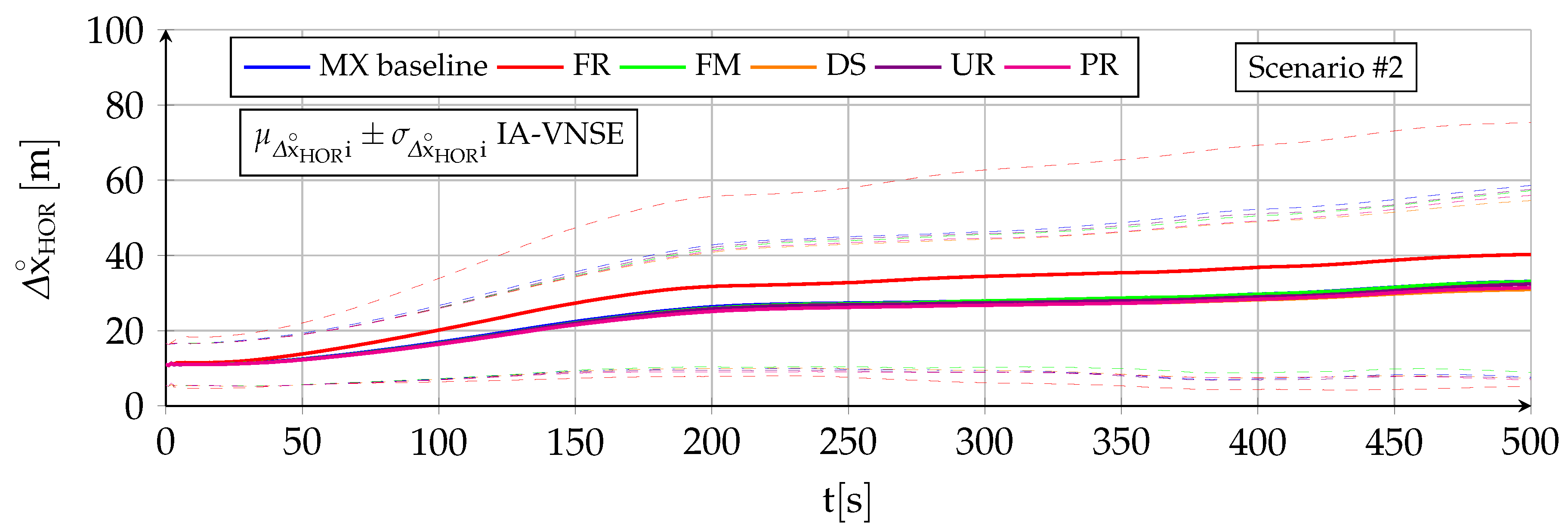
7.3. Horizontal Position Estimation

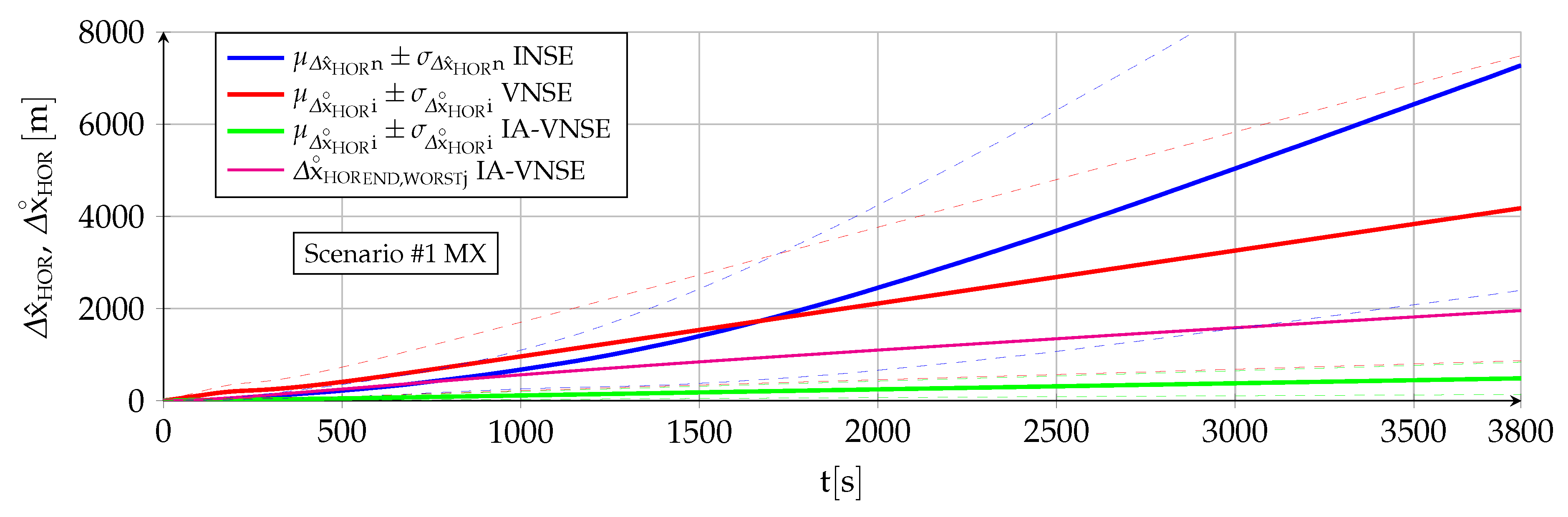
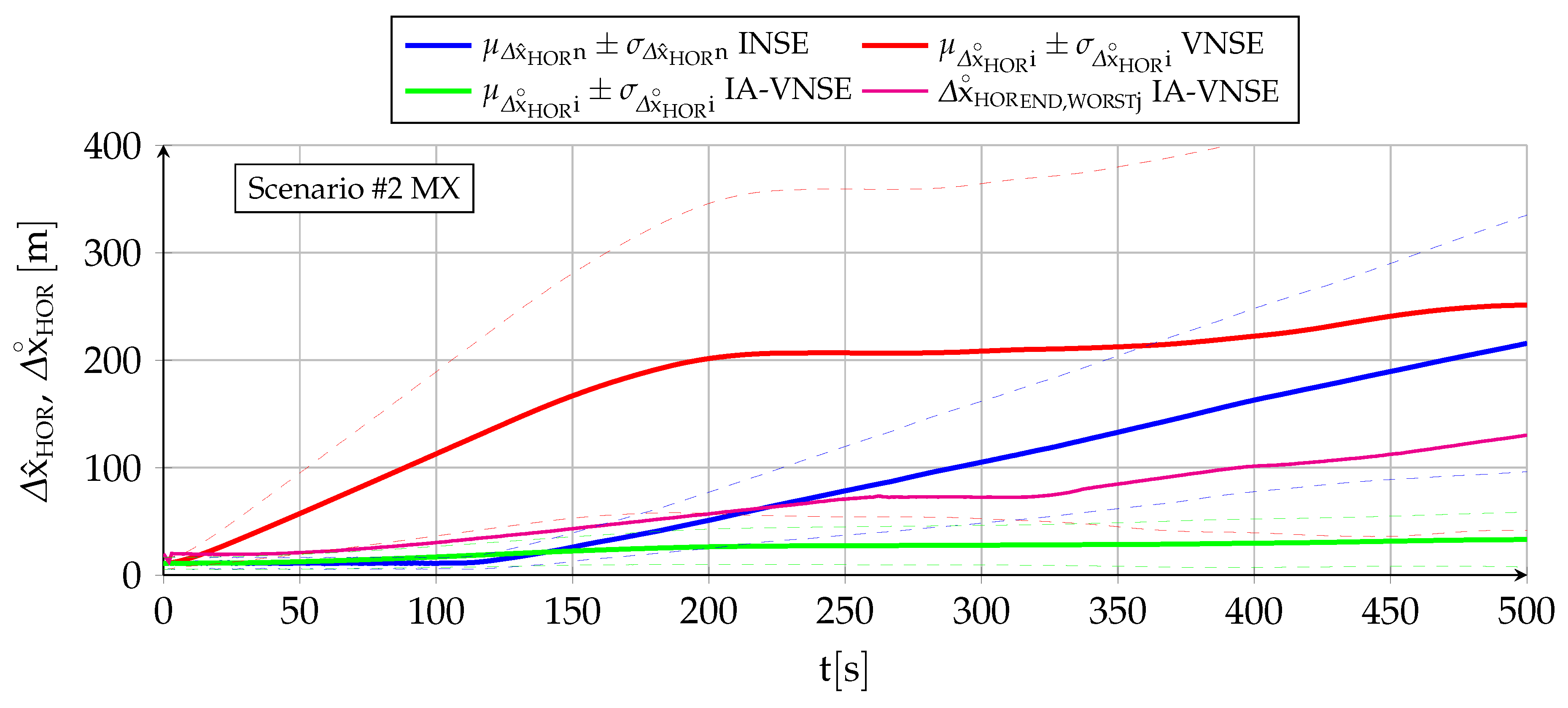
The horizontal position estimation capabilities of the INS, VNS, and IA-VNS share the fact that all of them exhibit an unrestrained drift or growth with time, as shown in Figure 13 and Figure 14. The errors obtained at the end of both scenarios are shown in Table 6, following the same scheme as in previous sections. While the approximately linear INS drift appears when integrating the bounded ground velocity errors [6], the visual drifts (both VNS and IA-VNS) originate in the slow accumulation of errors caused by the concatenation of the relative poses between consecutive images without absolute references, but also show a direct relationship with the scale error committed when estimating the aircraft height over the terrain during the initial homography (Appendix C).

In the case of the VNS (red lines), its scenario ${\displaystyle \#1}$ horizontal position estimations appear to be significantly more accurate than those of the INS (blue lines). Note, however, that the ideal image generation process discussed in Section 6 implies that the simulation results should be treated as a best case only, and that the results obtained in real world conditions would likely imply a higher horizontal position drift. The drift experienced by the VNS in Figure 14 (scenario ${\displaystyle \#2}$) also shows the same diminution in its slope in the second half of the scenario discussed in previous sections, which is attributed to previously mapped terrain points reappearing in the camera field of view as a consequence of the continuous turns present in scenario ${\displaystyle \#2}$. Additionally, notice how the VNSE starts growing at the beginning of the scenario, while the INSE only starts doing so after the GNSS signals are lost at ${\displaystyle {\mathrm{t}}_{\mathrm{GNSS}}=100\mathrm{s}}$ [6].

The IA-VNS (green lines) results in major horizontal position estimation improvements over the VNS. The final horizontal position error mean ${\displaystyle {\mu }_{\mathrm{END}\mathit{\Delta }{\stackrel{\circ }{\mathrm{x}}}_{\mathrm{HOR}}}}$ diminishes from ${\displaystyle 3.82}$ to ${\displaystyle 0.46\%}$ for scenario ${\displaystyle \#1}$, and from ${\displaystyle 1.77}$ to ${\displaystyle 0.23\%}$ for scenario ${\displaystyle \#2}$. The repeatability of the results also improves, as the final standard deviation ${\displaystyle {\sigma }_{\mathrm{END}\mathit{\Delta }{\stackrel{\circ }{\mathrm{x}}}_{\mathrm{HOR}}}}$ falls from ${\displaystyle 2.73}$ to ${\displaystyle 0.31\%}$ and from ${\displaystyle 1.48}$ to ${\displaystyle 0.18\%}$ for both scenarios. Note that although these results may be slightly optimistic due to the optimized image generation process, they are much more accurate than those obtained with the INS, for which the error mean and standard deviation amount to ${\displaystyle 7.10}$ and ${\displaystyle 5.69\%}$ for scenario ${\displaystyle \#1}$, and ${\displaystyle 1.52}$ and ${\displaystyle 0.86\%}$ in case of scenario ${\displaystyle \#2}$.

It is interesting to remark how the prior based pose optimization described in Section 5, an algorithm that adjusts the aircraft pitch and bank angles based on deviations between the visually estimated pitch angle, bank angle, and geometric altitude, and their inertially estimated counterparts, is capable of not only improving the visual estimations of those three variables, but doing so with a minor improvement in the body yaw estimation and an extreme reduction in the horizontal position error. When the cost function within an optimization algorithm is modified to adjust certain target components, the expected result is that this can be achieved only at the expense of the accuracy in the remaining target components, not in addition to it. The reason why in this case all target components improve lies in that the adjustment creates a better fit between the ground terrain and associated 3D points depicted in the images on one side, and the estimated aircraft pose indicating the position and attitude from where the images are taken on the other.

8. Influence of Terrain Type

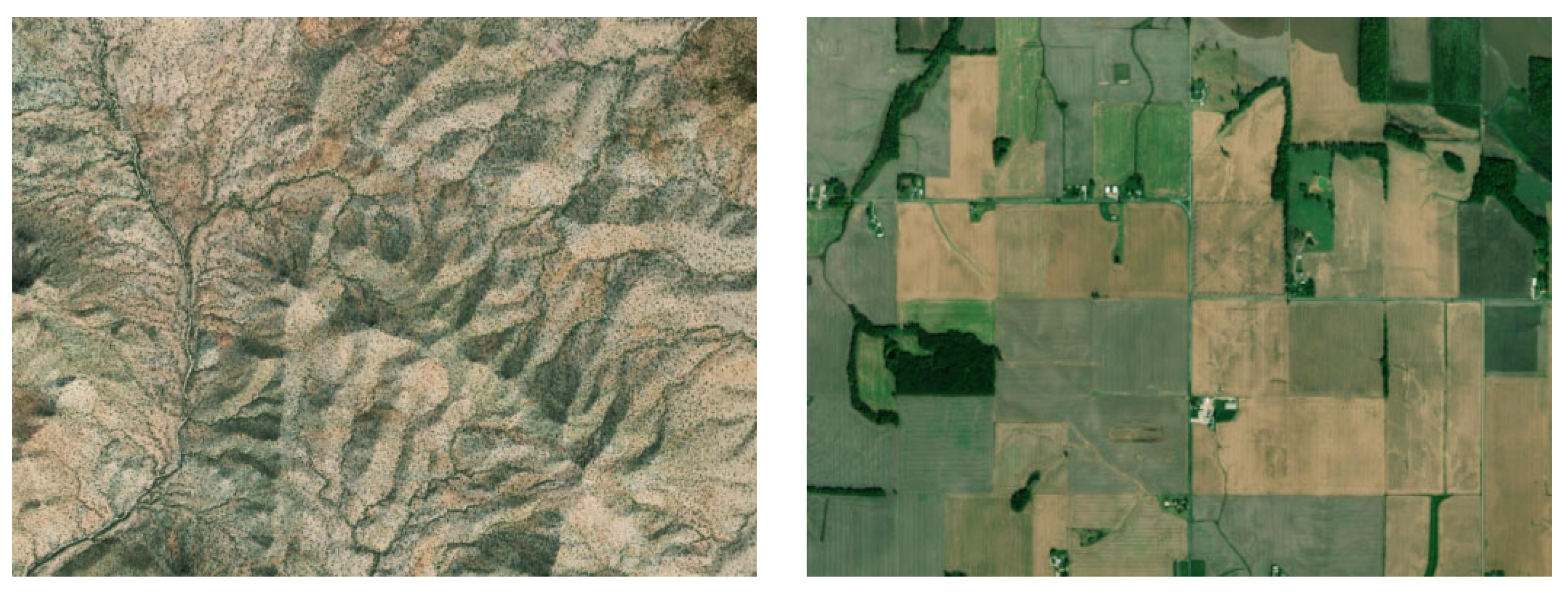
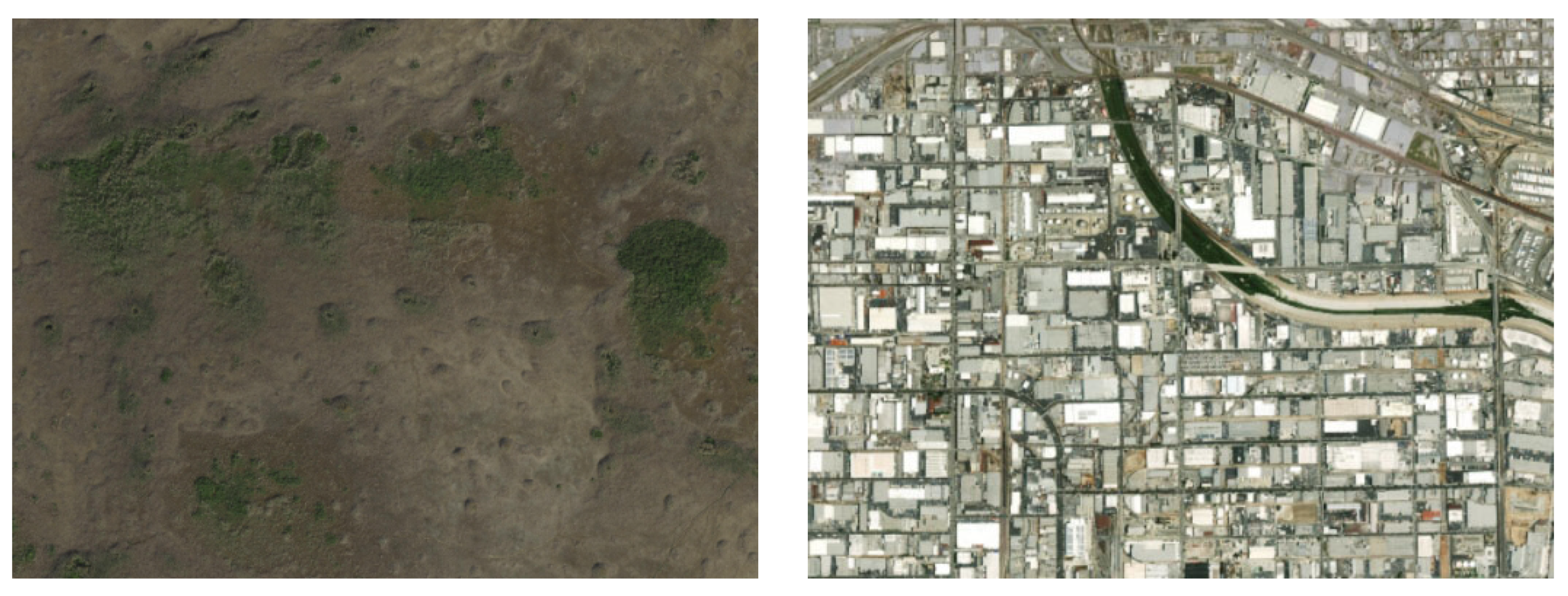
The type of terrain overflown by the aircraft has a significant influence on the performance of the visual navigation algorithms, which can not operate unless the feature detector is capable of periodically locating features in the various keyframes, and which also requires the depth filter to correctly estimate the 3D terrain coordinates of each feature (Appendix C). The terrain texture (or lack of) and its elevation relief are, hence, the two most important characteristics in this regard. To evaluate its influence, each of the scenario #1 100 Monte Carlo runs are executed flying above four different zones or types of terrain, intended to represent a wide array of conditions; images representative of each zone as viewed by the onboard camera are included below. The use of terrains that differ in both their texture and vertical relief is intended to provide a more complete validation of the proposed algorithms. Note that the only variation among the different simulations is the terrain type, as all other parameters defining each scenario (mission, aircraft, sensors, weather, wind, turbulence, geophysics, initial estimations) are exactly the same for all simulation runs.

• The “desert” (DS) zone (left image within Figure 15) is located in the Sonoran desert of southern Arizona (USA) and northern Mexico. It is characterized by a combination of bajadas (broad slopes of debris) and isolated very steep mountain ranges. There is virtually no human infrastructure or flat terrain, as the bajadas have sustained slopes of up to ${\displaystyle 7^{\circ }}$. The altitude of the bajadas ranges from ${\displaystyle 300}$ to ${\displaystyle 800\mathrm{m}}$ above MSL, and the mountains reach up to ${\displaystyle 800\mathrm{m}}$ above the surrounding terrain. Texture is abundant because of the cacti and the vegetation along the dry creeks.
• The “farm” (FM) zone (right image within Figure 15) is located in the fertile farmland of southeastern Illinois and southwestern Indiana (USA). A significant percentage of the terrain is made of regular plots of farmland, but there also exists some woodland, farm houses, rivers, lots of little towns, and roads. It is mostly flat with an altitude above MSL between ${\displaystyle 100}$ and ${\displaystyle 200\mathrm{m}}$, and altitude changes are mostly restricted to the few forested areas. Texture is non-existent in the farmlands, where extracting features is often impossible.
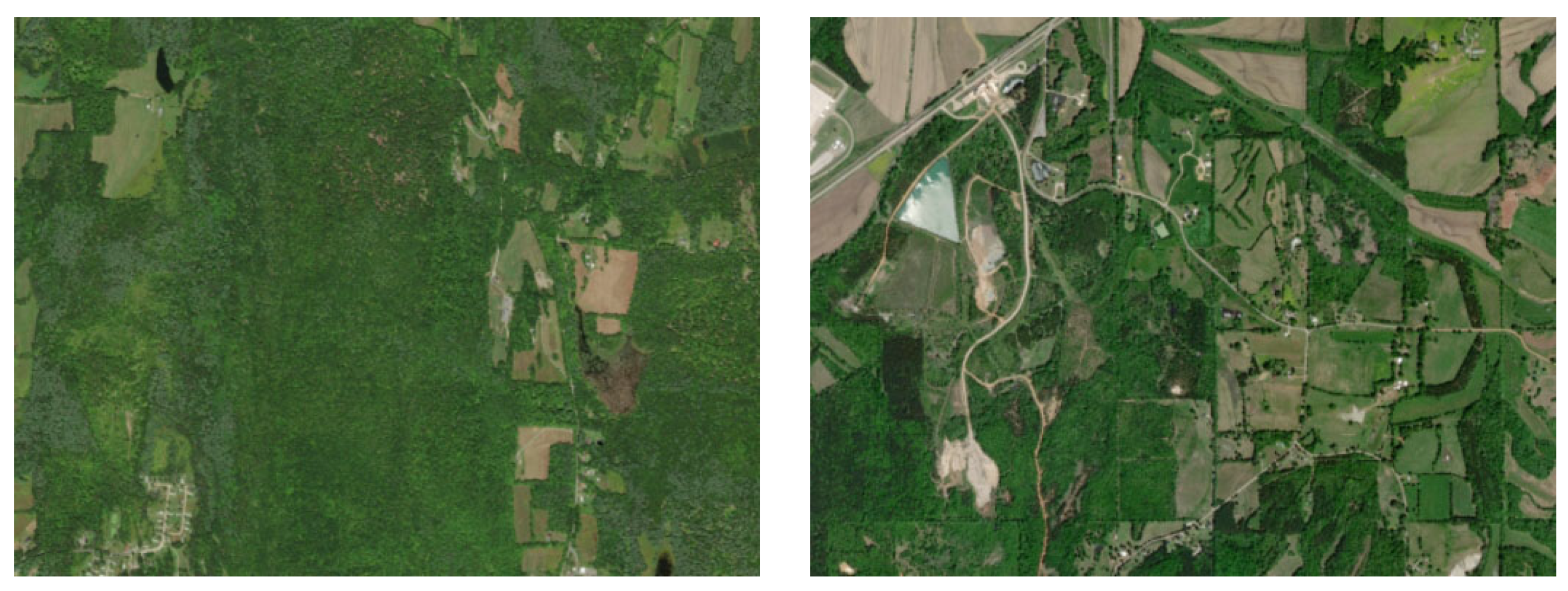
• The “forest” (FR) zone (left image within Figure 16) is located in the deciduous forestlands of Vermont and New Hampshire (USA). The terrain is made up of forests and woodland, with some clearcuts, small towns, and roads. There are virtually no flat areas, as the land is made up by hills and small to medium size mountains that are never very steep. The valleys range from ${\displaystyle 100}$ to ${\displaystyle 300\mathrm{m}}$ above MSL, while the tops of the mountains reach ${\displaystyle 500}$ to ${\displaystyle 900\mathrm{m}}$. Features are plentiful in the woodlands.
• The “mix” (MX) zone (right image within Figure 16) is located in northern Mississippi and extreme southwestern Tennessee (USA). Approximately half of the land consists of woodland in the hills, and the other half is made up by farmland in the valleys, with a few small towns and roads. Altitude changes are always present and the terrain is never flat, but they are smaller than in the DS and FR zones, with the altitude oscillating between ${\displaystyle 100}$ and ${\displaystyle 200\mathrm{m}}$ above MSL.

The short duration and continuous maneuvering of scenario #2 enables the use of two additional terrain types. These two zones are not employed in scenario #1 because the authors could not locate wide enough areas with a prevalence of this type of terrain (note that scenario #1 trajectories can conclude up to ${\displaystyle 125\mathrm{km}}$ in any direction from its initial coordinates, but only ${\displaystyle 12\mathrm{km}}$ for scenario #2).

• The “prairie” (PR) zone (left image within Figure 17) is located in the Everglades floodlands of southern Florida (USA). It consists of flat grasslands, swamps, and tree islands located a few meters above MSL, with the only human infrastructure being a few dirt roads and landing strips, but no settlements. Features may be difficult to obtain in some areas due to the lack of texture.
• The “urban” (UR) zone (right image within Figure 17) is located in the Los Angeles metropolitan area (California, USA). It is composed by a combination of single family houses and commercial buildings separated by freeways and streets. There is some vegetation but no natural landscapes, and the terrain is flat and close to MSL.

The MX terrain zone is considered the most generic and hence employed to evaluate the visual algorithms in Section 7. Although scenario #2 also makes use of the four terrain types listed for scenario #1 (DS, FM, FR, and MX), it is worth noting that the variability of the terrain is significantly higher for scenario #1 because of the bigger land extension covered. The altitude relief, abundance or scarcity of features, land use diversity, and presence of rivers and mountains is, hence, more varied when executing a given run of scenario #1 over a certain type of terrain, than when executing the same run for scenario #2. From the point of view of the influence of the terrain on the visual navigation algorithms, scenario #1 should theoretically be more challenging than #2.

Table 7. Influence of terrain type on final horizontal position IA-VNSE for scenario ${\displaystyle \#1}$ (100 runs). The most important metrics appear in bold.

Scenario ${\displaystyle \#1}$ Zone		MX		FR		FM		DS
${\displaystyle \mathit{\Delta }{\stackrel{\mathbf{\circ }}{\mathbf{x}}}_{\mathbf{HOR}}\left({\mathbf{t}}_{\mathbf{END}}\right)}$		${\displaystyle \left[\mathbf{m}\right]}$	${\displaystyle \left[\mathbf{\%}\right]}$	${\displaystyle \left[\mathbf{m}\right]}$	${\displaystyle \left[\mathbf{\%}\right]}$	${\displaystyle \left[\mathbf{m}\right]}$	${\displaystyle \left[\mathbf{\%}\right]}$	${\displaystyle \left[\mathbf{m}\right]}$	${\displaystyle \left[\mathbf{\%}\right]}$
IA-VNSE	mean	488	0.46	566	0.53	489	0.45	514	0.48
	std	350	0.31	406	0.38	322	0.28	352	0.31
	max	1957	1.48	2058	1.71	1783	1.34	1667	1.37

and Figure 18 show the horizontal position IA-NVSE for scenario ${\displaystyle \#1}$ and all terrain types.

Table 8. Influence of terrain type on final horizontal position IA-VNSE for scenario ${\displaystyle \#2}$ (100 runs). The most important metrics appear in bold.

Scenario ${\displaystyle \#2}$ Zone		MX		FR		FM		DS		UR		PR
${\displaystyle \mathit{\Delta }{\stackrel{\mathbf{\circ }}{\mathbf{x}}}_{\mathbf{HOR}}\left({\mathbf{t}}_{\mathbf{END}}\right)}$		${\displaystyle \left[\mathbf{m}\right]}$	${\displaystyle \left[\mathbf{\%}\right]}$	${\displaystyle \left[\mathrm{m}\right]}$	${\displaystyle \left[\mathbf{\%}\right]}$	${\displaystyle \left[\mathbf{m}\right]}$	${\displaystyle \left[\mathbf{\%}\right]}$	${\displaystyle \left[\mathbf{m}\right]}$	${\displaystyle \left[\mathbf{\%}\right]}$	${\displaystyle \left[\mathbf{m}\right]}$	${\displaystyle \left[\mathbf{\%}\right]}$	${\displaystyle \left[\mathbf{m}\right]}$	${\displaystyle \left[\mathbf{\%}\right]}$
IA-VNSE	mean	33	0.23	40	0.28	33	0.23	31	0.22	32	0.23	31	0.22
	std	26	0.18	35	0.24	24	0.17	24	0.17	25	0.18	25	0.17
	max	130	0.98	188	1.29	117	0.85	114	0.86	128	0.96	119	0.90

and Figure 19 do the same for scenario ${\displaystyle \#2}$.

The influence of the terrain type on the horizontal position IA-VNSE is very small, with slim differences among the various evaluated terrains. The only terrain type that clearly deviates from the others is FR, with slight but consistently worse horizontal position estimations for both scenarios. This behavior stands out as the abundant texture and continuous smooth vertical relief of the FR terrain is a priori beneficial for the visual algorithms.

Although beneficial for the SVO pipeline, the more pronounced vertical relief of the FR terrain type breaches the flat terrain assumption of the initial homography (Appendix C), hampering its accuracy, and, hence, results in less precise initial estimations, including that of the scale. The IA-VNS has no means to compensate the initial scale errors, which remain approximately equal (percentage wise) for the full duration of both scenarios.

A similar but opposite reasoning is applicable to the FM type and in a lesser degree to the UR and PR types. Although a flat terrain in which all terrain features are located at a similar altitude is detrimental to the overall accuracy of SVO, and results in slightly worse body attitude and vertical position estimations, it is beneficial for the homography initialization and the scale determination, resulting in consistently more accurate horizontal position estimations.

9. Summary of Results

This article proposes a Semi-Direct Visual Odometry (SVO)-based Inertially Assisted Visual Navigation System (IA-VNS) installed onboard a fixed wing autonomous UAV that takes advantage of the GNSS-Denied estimations provided by an Inertial Navigation System (INS) to assist the visual pose optimization algorithms. The method is inspired in a Proportional Integral (PI) control loop, in which the inertial attitude and altitude outputs act as targets to ensure that the visual estimations do not deviate in excess from their inertial counterparts, resulting in major improvements when estimating the aircraft horizontal position without the use of GNSS signals. The results obtained when applying the proposed algorithms to high fidelity Monte Carlo simulations of two scenarios representative of the challenges of GNSS-Denied navigation indicate the following:

• The body attitude estimation shows significant quantitative improvements over a standalone Visual Navigation System (VNS) in both pitch and bank angle estimations, with no negative influence on the yaw angle estimations. A small amount of drift with time is present, and can not be fully eliminated. Body pitch and bank angle estimations do not deviate in excess from their INS counterparts, while the body yaw angle visual estimation is significantly more accurate than that obtained by the INS.
• The vertical position estimation shows major improvements over that of a standalone VNS, not only quantitatively but also qualitatively, as drift is fully eliminated. The visual estimation does not deviate in excess from the inertial one, which is bounded by atmospheric physics.
• The horizontal position estimation, whose improvement is the main objective of the proposed algorithm, shows major gains when compared to either the standalone VNS or the INS, although drift is still present.

In addition, although the terrain texture (or lack of) and its elevation relief are key factors for the visual odometry algorithms, their influence on the aircraft pose estimation results are slim, and the accuracy of the IA-VNS does not vary significantly among the various evaluated terrain types.

10. Conclusions

The proposed inertially assisted VNS (IA-VNS), which in addition to the images taken by an onboard camera also relies on the outputs of an INS specifically designed for the challenges faced by autonomous fixed wing aircraft that encounter GNSS-Denied conditions, possesses significant advantages in both accuracy and resilience when compared with a standalone VNS, the most important of which is a major reduction in its horizontal position drift independently of the terrain type overflown by the aircraft. The proposed IA-VNS can significantly increase the possibilities of the aircraft safely reaching the vicinity of the intended recovery location upon the loss of GNSS signals, from where it can be landed by remote control.